Introduction
Snow and ice cover 98% of all surfaces in Antarctica and form a major component in the climate system of the earth (Bindschadler Reference Bindschadler1998). This vast ice sheet results in strong radiative heat loss, which affects near-surface conditions since there is a close interaction between the radiation climate and boundary-layer dynamics (Van den Broeke Reference Van Den Broeke2004b). In addition, the mass balance of the Antarctic regulates the mean global sea level elevation (Rignot & Thomas Reference Rignot and Thomas2007). The surface of the ice sheet is formed almost completely of seasonal snow, which easily responds to changes in environmental conditions. Therefore, studying the spatiotemporal variations in the physical properties of the Antarctic snow cover is crucial. The buried individual snow layers become transformed into ice and record past weather and climate conditions in terms of local temperature, precipitation, and aerosol fluxes of marine, volcanic, terrestrial, cosmogenic and anthropogenic origin (Petit et al. Reference Petit, Jouzel, Raynaud, Barkov, Barnola, Basile, Bender, Chappellaz, Davis, Delaygue, Delmotte, Kotlyakov, Legrand, Lipenkov, Lorius, Pépin, Ritz, Saltzman and Stievenard1999). Antarctica also provides a unique environment in which to study the snow cover, because it has the cleanest atmospheric environment available on Earth (Legrand & Mayewski Reference Legrand and Mayewski1997).
The net accumulation rate and the variability of the snow surface are crucial for cover and climate models in Antarctica (e.g. Van Lipzig et al. Reference Van Lipzig, van Meijgaard and Oerlemans2002a, Reference Van Lipzig, van Meijgaard and Oerlemans2002b, Liston & Elder Reference Liston and Elder2006). These models are the key to understanding the current and past relations between the global climate and the Antarctic ice sheet. The spatial variations in snow accumulation in Dronning Maud Land (DML) are rather well known. The yearly snow accumulation has been studied through stake surveys, oxygen isotope measurements, firn cores, radar profiling, and sonic altimeters (Isaksson Reference Isaksson1992, Isaksson & Karlén Reference Isaksson and Karlén1994a, Reference Isaksson and Karlén1994b, Isaksson et al. Reference Isaksson, Karlén, Gundestrup, Mayewski, Whitlow and Twickler1996, Richardson et al. Reference Richardson, Aarholt, Hamran, Holmlund and Isaksson1997, Kärkäs et al. Reference Kärkäs, Granberg, Lavoie, Kanto, Rasmus and Leppäranta2002, Reference Kärkäs, Martma and Sonninen2005, Richardson-Näslund Reference Richardson-Näslund2004, Van den Broeke et al. Reference Van Den Broeke, Reijmer and van De Wal2004a, Granberg et al. Reference Granberg, Cliche, Mattila, Kanto and Leppäranta2009, Boening et al. Reference Boening, Lebsock, Landerer and Stephens2012). Snowdrift, sublimation, and melt-freeze cycles are known to occur and affect the oxygen and hydrogen isotope ratios, as well as the concentrations of fallen impurities on the snow surface (Johnsen Reference Johnsen1977, Schlosser & Oerter Reference Schlosser and Oerter2002). Also the relationships between the spatial variations in snow accumulation and the katabatic outflow have long been recognized, but are poorly understood (Gow & Rowland Reference Gow and Rowland1965, Melvold et al. Reference Melvold, Hagen, Pinglot and Gundestrup1998).
Several surface heat balance investigations have been performed in western DML (Bintanja et al. Reference Bintanja, Jonsson and Knap1997, Reijmer & Oerlemans Reference Reijmer and Oerlemans2002, Van den Broeke et al. Reference Van Den Broeke, Reijmer, van As, van De Wal and Oerlemans2005, Reference Van Den Broeke, Reijmer, van As and Boot2006), but far fewer snow temperature records are available (Granberg et al. Reference Granberg, Cliche, Mattila, Kanto and Leppäranta2009). Snow surface layer temperature data provide an independent system for mapping the net surface heat balance and guide the coupling between ice sheet thermodynamics and atmospheric weather conditions. The thermal regime is strongly influenced by the katabatic outflow from the interior regions of Antarctica and the synoptic pressure gradient enhances the east–west-directed component of the katabatic wind (Noone et al. Reference Noone, Turner and Mulvaney1999, Van den Broeke et al. Reference Van Den Broeke, Winther, Isaksson, Pinglot, Karlöf, Eiken and Conrads1999). The physical properties of the snowpack at the western DML are also relatively well known through previous studies (e.g. Rasmus et al. Reference Rasmus, Granberg, Kanto, Kärkäs, Lavoie and Leppäranta2003, Kanto Reference Kanto2006).
In the Finnish Antarctic Research Program (FINNARP) 2009 expedition to western DML, during the summer of 2009/10, two automatic snow temperature stations were deployed, separated by 50 km distance (Fig. 1). Snow station 1 was deployed on the ice shelf and snow station 2 on the ice sheet south of the grounding line. The locations were 40 km north-west and 10 km south-east, respectively, from the Finnish research station Aboa (73°02.5′S, 13°24.4′W) on the Basen nunatak (unofficial name), about 120 km inland from the edge of the ice shelf. The data from the snow stations were retrieved one year later. The experiment had two objectives. The first was to build and test an improved sensor system that would operate in the challenging Antarctic environment. An earlier effort, which was partly a failure, since the longest temperature record extended only six months (Granberg et al. Reference Granberg, Cliche, Mattila, Kanto and Leppäranta2009), provided us with important information about the technical requirements of snow stations. The second, primary objective was to analyse the mass and heat budget of the snow surface layer. This included snow net accumulation, with the timing and magnitude of the accumulation events, variability of temperature with time and depth, and heat fluxes in the surface snow layer. Previous studies have shown that the snow surface level is almost always identifiable from the temperature gradient profiles (Granberg & Irwin Reference Granberg and Irwin1990, Granberg et al. Reference Granberg, Cliche, Mattila, Kanto and Leppäranta2009). Thus the snow station provides a method for measuring the snow accumulation. Its advantages, compared with a sonic altimeter used in some automatic weather stations, include building cost, maintenance and power requirement. The heat flux through the surface snow layer can also be analysed from the temperature data.
Map of the research area with the snow station locations indicated.

Here we present the instrumentation and the results of the automatic snow station experiment. Both stations were fully operational at the time of data retrieval and had recorded data over the entire year. The methods are presented first. Snow mass balance is then analysed based on the snow-air interface identified from the temperature data. The temperature data are analysed for monthly statistical characteristics, variance spectra, heat content of the surface snow layer, and heat flow through this layer. These snow stations are useful for spatial monitoring of the physics of the snow surface layer and for the mass and heat fluxes at the surface.
Instruments and methods
Description of study site
The study sites are located in western DML, East Antarctica (Fig. 1). The fieldwork was conducted from the Finnish research station Aboa (73°02.5′S, 13°24.4′W; altitude 485 m a.s.l.), located on the Basen nunatak (584 m a.s.l.). Basen is the most northern nunatak of the 130 km long Vestfjella mountain range (unofficial name) near the grounding line of the Riiser-Larsen Ice Shelf. In the Vestfjella area the average altitude is about 400 m a.s.l. and blue ice areas are common (Holmlund & Näslund Reference Holmlund and Näslund1994). The Riiser-Larsen Ice Shelf north-west of Aboa floats and slopes gently from an elevation of slightly over 200 m near Aboa to < 50 m at the shelf edge. The Heimefrontfjella Range is situated about 150 km inland from Vestfjella and partly blocks the ice flow from Amundsenisen.
Reijmer & Oerlemans (Reference Reijmer and Oerlemans2002) showed that the near-surface climate in DML is determined by a combination of katabatic winds and synoptic winds forced by transient cyclones travelling eastwards parallel to the coastline. The high-elevation areas to the south-east of the Vestfjella mountain range are less affected by the changing sea ice cover and cyclonic activity than the coastal area (King & Turner Reference King and Turner1997). The annual mean air temperature on the ice shelf is -19°C, behind the grounding line it is -16°C, and on the high-elevation areas south of Vestfjella it is -20°C (Reijmer & Oerlemans Reference Reijmer and Oerlemans2002). Kärkäs (Reference Kärkäs2004) reported that the monthly mean air temperatures vary from -5.2°C in January to -21.9°C in August according to the automatic weather station (AWS) (497 m a.s.l.) at the Aboa station.
Technical specification of snow stations
The snow stations were built, following instructions found in ‘The temperature handbook’ by Omega Engineering Inc, Stamford, CT, USA (Omega 1992) with some small modifications. Here we describe in general how the snow stations were built. More detailed instructions and a list of needed parts can be found in Omega (1992). Both snow stations are comprised of 20 mm diameter rigid plastic tubing, 4.5 m long, inside of which was placed a 20-pair cable, about 8 m long. The cable was longer than the plastic tubing to enable it to reach the logger box. To minimize radiation errors, the plastic tubing was manufactured from white high-reflectance plastic and the 20-pair cable was also white. Some radiation error could probably have resulted in calm conditions with strong sunshine during the summer months. Therefore, the daytime temperatures may be biased, but at night, when the sun was close to the horizon, the snow surface can be detected. The rigid plastic tubing provided support for the cable to which all the thermistors were attached. Snow station 1 had 16 thermistors and snow station 2 had 15. The distance between the sensors varied from 8–52 cm. The thermistor has a resistance that varies inversely with the temperature: if the temperature increases, the resistance of the thermistor decreases. By measuring the temperature and the associated resistance of each thermistor in an ice bath, we could accurately record the response of each thermistor to changes in the temperature.
The cable with the thermistors was connected to the data logger, with each thermistor connected to its own channel. We used a CR1000 data logger (Campbell Scientific Ltd) because it is resistant to low-temperature-conditions (Vehviläinen Reference Vehviläinen2010). Programming the logger and data retrieval were done via an RS232 interface and the logger was placed in an insulated plastic box that could withstand the weight of the snowpack. For the power supply we used 12-V DC lead-acid batteries that were placed in an insulated wooden box. We estimated that a 24 ampere-hour (Ah) battery would last about 1000 days, but the extreme low temperatures (-40°C) could have an effect on the electric current. To ensure that the batteries would deliver the necessary current for an entire year or longer, in case the planned retrieval next year was impossible to carry out, we used a 60 Ah battery at snow station 1 and a 48 Ah battery at snow station 2.
Measurements and deployment
The snow stations were installed in open snowfields that were relatively flat and without any visible crevasses for at least a 10 km radius to minimize the effects of the local topography on the snow accumulation. Their positions were selected to represent gradation in altitude and distance from the ocean (Table I). The goal was to find a site representative of a larger area (ice shelf or continental ice sheet), thus for example, sloping surfaces near the grounding line are not good because the snow accumulation may be completely different there and not representative of the larger area. In this way we can use the data in snow cover and climate modelling studies.
General information on the positions of the snow stations. Dates are given as day.month.year.

Snow station 1 was installed on the Riiser-Larsen Ice Shelf 40 km north-west of Aboa and snow station 2 was installed next to AWS 5 on the continental ice sheet 10 km south-east of Aboa. Unfortunately, snow station 1 was installed accidentally on a sloping surface, on the lee side relative to the prevailing wind direction in that area, and this caused major problems in interpreting the temperature data. Flagged bamboo poles, about 1.5 m long, were used to facilitate finding the stations one year later. The co-ordinates of the snow stations were obtained with a Garmin GPS 12 XL hand-held navigator with accuracy of 10 m.
A Kovacs MARK II coring system was used to drill a 4 m deep vertical hole. The sensor rod was inserted into the hole and the sensors were turned to face the wall of the hole to connect with the undisturbed snowpack. The hole was later filled with snow. Bamboo poles were used to pack the snow tightly so that the temperature sensors would have a good connection with the snowpack. Wooden spikes and a rope were used to support the sensor rod so that it would not sway or break in the wind. The depths of all sensors for both stations after the installation are marked in Table II. The minus sign indicates that the sensor was above the snow surface (0 m). The snow stations were programmed by means of a portable laptop before the data logger and battery boxes were buried 0.5 m below the snow surface a few metres away from the sensor rod. The snow stations measured the temperature at 5 min intervals, and the average value from three measurements was stored in the data logger every 15 min. With these settings, there was enough space for 1.5 years of data.
Sensor depths in metres after installation. The minus sign indicates that the sensor was above the snow surface (0 m).

At each site a 1.5 m deep snow pit was dug during installation and retrieval to record the physical properties of the snowpack. The snow pit in 2010 was dug 600 m from snow station 1 for safety reasons (small crevasses visible). The physical characterization of snow stratigraphy was done at 10 cm vertical resolution. The size and shape of the snow grains were determined, using an 8x magnifier and a millimetre-scale grid. The snow-type classification followed ‘The international classification for seasonal snow on the ground’ issued by the International Association of Cryospheric Sciences (IACS) (Fierz et al. Reference Fierz, Armstrong, Durand, Etchevers, Greene, McClung, Nishimura, Satyawali and Sokratov2009). The snow grain size reported is the greatest diameter of a grain. The temperature profiles were measured, using a digital thermometer (EBRO TLC1598, Argus Realcold Ltd, Auckland, New Zealand) with resolution of 0.1°C and an accuracy of ± 0.2°C. The snow density was directly measured using a cylinder sampling kit with a volume of 250 cm3 (diameter 5 cm) and a Pesola spring balance with 5-g resolution. The accuracy was estimated as ± 10 kg m-3. The accumulation was measured from the snow samples and the bamboo poles installed next to the snow stations. To ensure minimal settling of the bamboo poles, they were hammered into the snow as deeply as possible without breaking them. Previous studies (e.g. Rasmus et al. Reference Rasmus, Granberg, Kanto, Kärkäs, Lavoie and Leppäranta2003, Kanto Reference Kanto2006) used the same method, which is a reliable way to measure the snow accumulation. The AWS 5 next to snow station 2 measured the height of the snow surface, using a SR 50 acoustic sensor (Campbell Scientific Ltd). The AWS 5 has measured meteorological quantities including air temperature, relative humidity, wind speed and short and longwave radiation since the summer of 1997 (Reijmer & Oerlemans Reference Reijmer and Oerlemans2002). In addition there was another AWS (AWS 4) on the ice shelf between 1997 and 2002. Data from AWS 4 were used to define the prevailing wind direction on the ice shelf. Automatic weather stations 4 and 5 were identical stations installed by the Institute for Marine and Atmospheric Research, Utrecht, the Netherlands (IMAU). Noteworthy for this study is that the uncertainty in the shortwave and longwave radiative fluxes measured by AWS 4 and 5 is estimated to be ± 10% and ± 20%, respectively, and the uncertainty in the relative humidity about 5% (Reijmer & Oerlemans Reference Reijmer and Oerlemans2002). Reijmer & Oerlemans (Reference Reijmer and Oerlemans2002) also noted that occasional occurrence of hoar on the sensors affected the observations.
Retrieval of stations
The first attempt to locate snow station 1 was made on 20 December 2010 on a field trip from Aboa to the shelf edge. All three bamboo poles were buried and snow station 1 could not be located. Snow pit measurements revealed that more than 1.5 m of new snow had accumulated during the previous 12 months. The second attempt to locate snow station 1 was made on 20 January 2011, and this time two bamboo poles were visible. We estimate that there had been a significant amount of snowmelt and sublimation during summer (from 10–30 cm) in the month between field trips. Data from the Aboa weather station revealed that the air temperature regularly rose above 0°C during this one month period. The Aboa weather station is 445 m higher than snow station 1. Automatic weather station 5 (310 m higher than snow station 1) also regularly recorded air temperatures above 0°C during this one month period. Therefore, we assumed that the air temperature at snow station 1 was above 0°C several times. Snow station 1 was fully operational, but we had to dismantle it, otherwise it would have become buried too deeply to be recovered in future.
Data were collected from snow station 2 on 21 January 2011. The station was fully operational and had stored data continuously without any interruptions, except a data gap caused by changing of the batteries (18–22 January 2010). The sensor rod was buried under the snow surface and had no visible influence on nearby snow accumulation. Snow station 2 was left to acquire more data and it was still operational in January 2013.
Data processing
Power spectra calculations and window functions
A power spectrum describes how the variance of a signal or time series is distributed with frequency and helps to analyse temporal behaviour and identify periodicities. Here the temperature spectra are basically compressed time series information describing the time scales of the variability of weather conditions, and, within the snow, the damping and phase shift of temperature signal that are dependent on the thermal properties of the snow. Window functions are used in harmonic analyses to reduce the undesirable effects related to spectral leakage. All window functions are designed to reduce the side lobes of the spectral output of fast Fourier transform (FFT) routines. While applying the window function reduces the side lobe leakage, it causes the main lobe to broaden, thus reducing the resolution (Kumar et al. Reference Kumar, Singh and Saxena2011). We used the Hamming and Blackman-Harris windows in calculating the power spectra, because these window functions were the best available for our needs (Fig. 2). The Hamming window is one of the most popular and most commonly used windows. It is optimized to minimize the maximum (nearest) side lobe and its shape is similar to that of a cosine wave (one period of a raised cosine). The Blackman-Harris window is also popular and is useful for single-tone measurement. The Blackman-Harris window is a generalization of the Hamming family and it has a wider main lobe and a lower maximum side lobe level than the Blackman window (see Fig. 2). The Blackman-Harris window is produced by adding more shifted normalized sinc functions and is less sensitive than the Hamming window. Performing the spectral analyses always involves a trade-off between resolving comparable strength signals with similar frequencies and resolving disparate strength signals with dissimilar frequencies. This trade-off occurs when the window function is chosen. Detailed descriptions of the Hamming and Blackman-Harris windows can be found in Harris (Reference Harris1974).
Graphical illustrations of the Hamming and Blackman-Harris windows.
Snow density profile
Simple methods can be used to interpret the snow data for heat budget and mass balance analyses. First, snow density is considered, a quantity necessary to examine the mass balance from the snow thickness data. We assumed that the monthly snow density profiles were similar from year to year, in order to simplify the transformation of net snow accumulation into mass balance. There were some small density variations in the near-surface layer, due to differences in snowfall, snowdrift, and temperature history, but these variations had only minor influences on the mass balance estimation. The influence to the mass balance estimation is less than 10% based on the density measurements (see Physical properties of the snowpack). Snow density increases with depth due to snow metamorphism, especially due to pressure of the overlying snow. The snow density profile ρ(z) was taken as (Schytt Reference Schytt1958):
 $$ \rho \left( z \right)\, = \,{{\rho }_{\rm{0}}}\, + \,\left( {{\rm{1}}\,{\rm{ - }}\,ex{{p}^{{\rm{ - }}\mu z}} } \right)\,\left( {{{\rho }_i}{\rm{ - }}{{\rho }_0}} \right), \eqno\rm$$
where ρ0 is the density at the surface, ρ i the ice density at deeper layers, μ the inverse vertical length scale of density increase, and z the depth. This equation was based on observations in DML and satisfies the differential equation in which the rate of change of density with depth equals μ(ρi-ρ). This can be transformed for the evolution of snow thickness as (Granberg et al. Reference Granberg, Cliche, Mattila, Kanto and Leppäranta2009):
 $$ \frac{{dh}}{{dt}}\, = \,{\rm{ - }}\gamma h\, + \,a^{\prime}, \eqno\rm$$
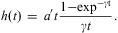
where t is time, γ is the compaction rate and a′ is the net accumulation rate. Assuming that a′ and γ are constants and h(0) = 0, the solution is:
 $$ h\left( t \right)\, = \,a^{\prime}t\frac{{{\rm{1 - }}{{{\exp }}^{{\rm{ - \gamma t}}}} }}{{\gamma t}}. \eqno\rm$$
The compaction rate can be numerically estimated when the snow density and accumulation rate are known. Equation (3) is used to transform a change in the thickness of a snow layer to change in the mass of snow. Taking γ as a constant limits the applicability of the solution to a surface layer < 10 m thick. Equation (3) results in an approximately linear density profile across the snow layer in the present study.
Snow temperature
The temperature data can be utilized to examine the thermal properties of snow and the heat flow in the snow. In the near-surface layer, snow density is approximately a constant and thus also is the thermal conductivity. The temperature T = T(t,z) then follows the heat diffusion equation:
 $$ \frac{{\partial T}}{{\partial t}}\, = \,D\frac{{{{\partial }^2} T}}{{\partial {{z}^2} }}\, + \,\kappa {{Q}_{\rm{0}}}\,\exp ({\rm{ - }}\kappa z), \eqno\rm$$
where D is the heat diffusion coefficient, κ the attenuation coefficient, and Q 0 the net solar radiation at the surface. The radiation term is missing in the polar night and in summer radiation is absorbed just below the surface and its penetration into snow is often neglected. Assuming a temperature boundary condition of a sine wave of frequency ω at the surface and constant T ∞ at infinite depth, the solution of Eq. (4) is (e.g. Paterson Reference Paterson1994):
 $$ T\left( {t,z} \right)\, = \,{{T}_\infty }\, + \,{\rm{\rDelta }}T{{e}^{{\rm{ - }}\lambda z}} \,\sin \left( {2\pi {\rm{\omega t - }}\lambda {\rm{z}}} \right). \eqno\rm$$
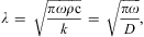
Here ΔT is the temperature amplitude at the surface, and
 $$ \lambda \, = \,\sqrt {\frac{{\pi {\rm{\omega }}\rho {\rm{c}}}}{k}} \, = \,\sqrt {\frac{{\pi {\rm{\omega }}}}{D}}, \eqno\rm$$
where c is the specific heat of ice and k the thermal conductivity. The diffusion coefficient (D = k/ρ c) can be estimated when the damping or phase shift (λ) at a fixed depth is known, and then the thermal conductivity (k) can be estimated, assuming the density of the snowpack is nearly constant in the top layer. Yen (Reference Yen1981) introduced the equation k = 2.22362ρ 1.885, where ρ is in Mg m-3 and k is in W °C-1 m-1.
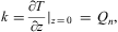
The heat flux from the snow cover can be estimated, using the temperature gradient in the top part of the snow cover:
 $$ k = \frac{{\partial T}}{{\partial z}}\left| {_{{z\, = \,0}} } \right.\, = \,{{Q}_n}, \eqno\rm$$
where Qn is the energy balance at the surface. Qn consists of four main components and can be expressed as:
 $$ {{Q}_n}\, = \,{{Q}_{SW}}\, + \,{{Q}_{LW}}\, + \,{{Q}_H}\, + \,{{Q}_{LE}}, \eqno\rm$$
in which QSW and QLW are the net shortwave and net longwave radiative fluxes, respectively, and QH and QLE are the turbulent fluxes of sensible and latent heat, respectively. The surface energy budget governs the near surface climate. The energy balance in DML is strongly associated with the strength of katabatic wind and hence with the surface slope. Generally in Antarctica the annual averaged energy balance is dominated by a negative radiative flux balanced mainly by the sensible heat flux (Reijmer & Oerlemans Reference Reijmer and Oerlemans2002).
Results
Physical properties of the snowpack
First we describe the snow pit profiles (crystal size and type, hand hardness, and stratigraphy) since they show whether dramatic changes have occurred in the snowpack that may impact the snow heat flux. For example, crystal size also affects the thermal conductivity. The measured snow pit profiles from snow station 1 in 2009 and 2010 are shown in Fig. 3. In 2009, two 1 mm thick ice lenses at depths of 72 cm and 140 cm were identified, and in 2010 there were two 1 mm thick ice lenses at depths of 28 cm and 48 cm. The snow pit in 2010 revealed an 80 cm thick hard refrozen layer and therefore there are no density values below 75 cm. The second week of January 2010 was quite warm and rain event (liquid precipitation) was also registered at the Aboa station. The liquid precipitation was probably the reason for the extremely thick refrozen layer. Above this layer there was a 2 cm thick depth hoar layer, and underneath there were again large rounded snow crystals.
Snow pit profiles for snow station 1 in 2009 and 2010. RGlr = large rounded particles, DHcp = depth hoar hollow cups, and MFcr = melt-freeze crust. Hand hardness test uses objects of decreasing areas and the index corresponds to the first object that can be gently pushed into the snow (fist = fist, 4-f = four fingers, 1-f = one finger, P = pencil and K = knife).
The measured snow density profiles and the density profile fits calculated using Eq. (1) for snow station 2 at the time of installation and retrieval are shown in Fig. 4, and the snow pit profiles are shown in Fig. 5. In 2009 there was one 2 mm thick ice lens at a depth of 85 cm, and in 2010 there were three 1 mm thick ice lenses at depths of 50 cm, 80 cm, and 125 cm. Two 1 cm thick ice layers were also identified at depths of 92 cm and 98 cm in 2010. There was no similar thick refrozen layer at snow station 2 as there was at snow station 1. This is probably due to the lower air and snow temperatures at station 2. Due to the lower air temperature the precipitation was probably wet snow or snow rather than entirely liquid water. Initially colder snowpack at snow station 2 prevented the liquid water/slush penetrating deeper parts and therefore preventing formation of the thick refrozen layer. It might also be that the amount of precipitation was smaller at snow station 2 than at snow station 1.
Snow density profiles for snow station 2, measured at the time of installation and retrieval from 1.5 m deep snow pits. The density profiles were calculated using Eq. (1) and the vertical length scale of density increase, μ-1, was 4.1 m in 2009 and 72 m in 2010.
Snow pit profiles for snow station 2 in 2009 and 2010. RGlr = large rounded particles, and RGxf = faceted rounded particles. Hand hardness test uses objects of decreasing areas and the index corresponds to the first object that can be gently pushed into the snow (fist = fist, 4-f = four fingers, 1-f = one finger, P = pencil and K = knife).
The vertical length scale of density increase, μ-1, was determined using Eq. (1). It gives the e-folding length of the difference between ρ0 and ρ i. At the depth of 3· μ-1, the density is 5% less than ice density. The value of μ-1 was 4.1 m in 2009 and 72 m in 2010. The surface density, ρ0, was 320 kg m-3 in 2009 and 400 kg m-3 in 2010. The variations in the density are due to the differences in snowfall and snowdrift. These variations attenuate with depth, due to the pressure caused by the overlying snowpack. The temperature also has an effect on the density: the higher the temperature, the quicker is the densification process. There are some differences in the density profiles between the snow station locations and years. The average surface density is 390 kg m-3 and at the depth of 1.5 m the average density is 460 kg m-3. The predominant size and shape of the snow crystals did not vary between locations or years: the crystals were normally small and rounded and their size was 1–1.5 mm.
Annual snow accumulation and mass balance
The annual net snow accumulation at each site was obtained from the stake measurements. Formally, it is given as the sum of the influences of precipitation P, sublimation E, and snowdrift R (deposition of snow). In Eq. (2), a′ is the sum of P, E, and R. Here, the net accumulation was measured by the elevation of the snow surface above a reference depth. The reference depth was set on 9 December to be 0 cm (the bamboo poles were installed). We calculated the monthly sublimation rates, E (mm in water), in 2010 from the AWS 5 data (Table III) using the bulk formula for turbulent transfer of water vapour with constant exchange coefficient of 1.3 x 10⁻³ (e.g. Curry & Webster Reference Curry and Webster1999). The monthly sublimation varied between 2.2 mm and 19.9 mm. The highest levels occurred during the summer months, December (19.9 mm) and January (18.3 mm) and the lowest ones in winter, July (2.2 mm) and August (2.4 mm), as expected. Most of the sublimation occurred in summer. A comparison between the bulk method and Monin-Obukhov similarity theory method showed no large differences in summer evaporation in a nearby nunatak (Leppäranta et al. unpublished). Sublimation is one component of the net snow accumulation and knowing it adds to the understanding of the mass balance of the ice sheet.
Monthly sublimation in 2010 calculated from the automatic weather station (AWS) 5 data (mm in water).

The snow surface level was almost always identifiable from the temperature gradient profiles. The temperature varied more slowly in the snowpack than in the air, due to the lower thermal diffusivity. The estimation is easier in the time series data, since the evolution of the temperature profile in snow and air is fairly different. The temperature gradient is different in air and snow, and to extrapolate them to the interface, the accuracy of the resulting surface elevation is dependent on the vertical spacing of the sensors. At these snow stations the spacing above the snow surface varied between 8 cm and 20 cm. Therefore, the accuracy was quite low, but observing how the temperature changed overnight revealed which sensors were buried under snow and when this occurred.
Figure 6 shows the temperature profiles of snow station 1 for three different dates at 03h00, 04h00, 05h00 and 06h00 Eastern European Time/Eastern European Summer Time (EET/EEST). We observed that on 4 March 2010 three sensors (-30, -20, and -9 cm) that were left above the snow surface were still above. Variation in the temperature during the three hour period was almost identical between these three sensors and the variation was much larger than in the two other sensors (9 cm and 29 cm). On 9 April 2010, sensor 3 (-9 cm at the time of installation) was buried under the snow. Variation in the temperature was much smaller than in the two uppermost sensors (-30 cm and -20 cm at the time of installation). This means that the snow surface was between -10 cm and -20 cm.There was no clear variation in temperatures between the three uppermost sensors on 16 May 2010. Sensors 2 (-20 cm) and 3 (-9 cm) were at least buried under the snow, but it is impossible to determine from the temperature data whether sensor 1 was buried. This is because sensor 1 (-30 cm) was the last sensor and we could not compare it with any other sensor above the snow surface. However, the snow surface height data from AWS 5 revealed that from 9 January to 16 May 2010 the total snow accumulation was 46 cm. Therefore, we assumed that sensor 1 (-30 cm) was also buried under snow, because AWS 5 was located only 50 km from snow station 1 and the overall snow accumulation was higher than at snow station 2.
Selected temperature profiles of snow station 1 at night. Time is Eastern European Time/Eastern European Summer Time (UTC +2/3). Vertical axis is height with respect to the surface at the date of installation (0 cm), where negative values indicate levels above the snow surface. Dates are given as day.month.year.
Figure 7 shows the temperature profiles of snow station 2 for three different dates at 03h00, 04h00, 05h00 and 06h00 EET/EEST. We observed that on 16 December 2009, sensor 4 (-6 cm at the time of installation) was already buried under snow. The temperature variations during the three hour period were much smaller than in the three uppermost sensors (-44, -36, and -26 cm at the time of installation). The same phenomenon was clearly visible in the temperature profile on 4 March 2010. There was no clear variation in the temperatures between the three uppermost sensors on 16 May 2010. Sensors 2, 3 and 4 were at least buried under snow, but again it is impossible to determine from the temperature data whether the uppermost sensor was buried also, but the snow surface elevation data from AWS 5 revealed that it was. In both Figs 6 & 7 the temperature profiles seem to be exponential and this is due to the differences in the thermal conductivities between air and snow.
Selected temperature profiles of snow station 2 at night. Time is Eastern European Time/Eastern European Summer Time (UTC +2/3). Vertical axis is height with respect to the surface at the date of installation (0 cm), where negative values indicate above the snow surface. Dates are given as day.month.year.
The net snow accumulation data from AWS 5 began only from 9 January 2010, due to technical problems, and the initial value is marked as 0 cm (Fig. 8). The AWS 5 data (sonic altimeter) revealed four major snow accumulation events between 9 January 2010 and 10 December 2010 (Figs 8–12). The first snow accumulation event occurred between 25 and 27 February 2010, adding 10 cm of new snow (Fig. 9). The second accumulation event occurred between 1 and 12 May 2010, with 36 cm of new snow (Figs 9 & 10), and the third event was the longest, lasting from 23 June–22 July 2010 (Fig. 10). During this period, the elevation of the snow surface varied greatly and the total snow accumulation was 29 cm. The last event occurred between 12 and 14 August 2010, bringing 13 cm of new snow (Fig. 11). From this event until 10 December, the height of the snow surface decreased by 11 cm, due to wind packing and sublimation. The annual net snow accumulation at snow station 2 measured from bamboo poles between 9 December 2009 and 10 December 2010, resulted in an 86 cm snow layer (345 mm water equivalent (w.e.)) (Table IV). The sonic altimeter measures the height of the snow surface and changes in the snow surface elevation provides the net snow accumulation (Reijmer & Van den Broeke Reference Reijmer and van Den Broeke2003).
Temperature profiles of the summer 1 segment from four sensors per snow station. The air temperature and net snow accumulation from automatic weather station (AWS) 5 at snow station 2 are also shown. The depths of the snow station 2 sensors at the end of the segment were -0.30 m (sensor 2), 0.40 m (sensor 6), 1.35 m (sensor 9), and 3.62 m (sensor 15). The depths are determined using the accumulation data from AWS 5.
Temperature profiles of the autumn segment from four sensors per snow station. The air temperature and net snow accumulation from automatic weather station (AWS) 5 at snow station 2 are also shown. The depths of the snow station 2 sensors at the end of the segment were 0.20 m (sensor 2), 0.90 m (sensor 6), 1.85 m (sensor 9), and 4.12 m (sensor 15). The depths are determined using the accumulation data from AWS 5.
Temperature profiles of the winter segment from four sensors per snow station. The air temperature and net snow accumulation from automatic weather station (AWS) 5 at snow station 2 are also shown. The depths of the snow station 2 sensors at the end of the segment were 0.46 m (sensor 2), 1.16 m (sensor 6), 2.11 m (sensor 9), and 4.38 m (sensor 15). The depths are determined using the accumulation data from AWS 5.
Temperature profiles of the spring segment from four sensors per snow station. The air temperature and net snow accumulation from automatic weather station (AWS) 5 at snow station 2 are also shown. The depths of the snow station 2 sensors at the end of the segment were 0.52 m (sensor 2), 1.22 m (sensor 6), 2.17 m (sensor 9), and 4.44 m (sensor 15). The depths are determined using the accumulation data from AWS 5.
Temperature profiles of the summer 2 segment from four sensors per snow station. The air temperature and net snow accumulation from automatic weather station (AWS) 5 at snow station 2 are also shown. The depths of the snow station 2 sensors at the end of the segment were 0.38 m (sensor 2), 1.08 m (sensor 6), 2.03 m (sensor 9), and 4.30 m (sensor 15). The depths are determined using the accumulation data from AWS 5.
Net accumulation (snow height in cm) measured from flagged bamboo poles with respect to the deployment day (marked as 0). Dates are given as day.month.year (- = no values available).

The snow compaction rate, γ, was determined numerically, using Eq. (3) and the measured density values. In Eq. (3) the term h(t)/a′t can be written as (ρm/ρ0)-1, where ρ m is the mean density of the accumulated snow layer. The annual net snow accumulation at snow station 2 was 86 cm, according to the bamboo poles. Using the measured density data, the annual net snow accumulation data and setting t = 1 y, the compaction rate became 0.0201 y-1. We estimated that the accuracy of the compaction rate was ± 0.02 y-1, based on the error margins of the density measurements.
To obtain the compaction rate for snow station 1 was more problematic, due to the thick refrozen layer. The density evolution there was a thermal-mechanical process. We did not measure the density profile for the refrozen layer. A snow pit dug only 600 m away from snow station 1 revealed that there the annual net snow accumulation was 79 cm (286 mm w.e.). Using the measured density data and the annual net snow accumulation data and setting t = 1 y, the compaction rate, γ, for that location was 0.675 ± 0.02 y-1. The high compaction rate is due to the low snow density measured at the surface. The local variations in the surface density had a greater influence on the estimated compaction rate than the accuracy based on the error margins of the density measurements.
Time variations in temperature
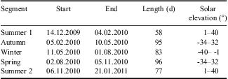
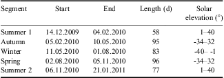
The temperature data were divided into five periods (summer 1, autumn, winter, spring, and summer 2) on the basis of the elevation of the sun (Table V). It was also easier to analyse the temperature data in smaller parts. Based on the vertical location at installation we selected four sensors from each station. The pairs were chosen such that the height at installation was similar. For station 1 sensors 1, 5, 9 and 16 were chosen, for station 2 sensors 2, 6, 9 and 15 were chosen. The heights at installation of these sensors are presented in Table II. Table VI shows the 2010 monthly mean temperature at snow station 2 calculated from the AWS 5 and snow station 2 observations. The surface temperature was calculated from the outgoing longwave radiation measured by AWS 5. The depth refers to the actual depths, not to the installation depths. The coldest month according to the air temperature was July, but the coldest month at the depth of 3.04 m was September. This is due the speed of the thermal diffusion in snow. This same phenomenon is seen in the warmest month (January vs February).
Dates (day.month.year), lengths, and the variations in the elevation of the sun for the five segments: summer 1, autumn, winter, spring, and summer 2. The minus sign indicates that the sun was below the horizon.
The 2012 monthly mean values of temperature (°C) at snow station 2. Air temperature and surface temperature are based on automatic weather station (AWS) 5 data, the snow temperatures are based on snow station 2 data (- = no values available). The depths are based on the accumulation data from AWS 5 and are approximately constants.

The temperature profiles of all segments for the four sensors from each snow station are shown in Figs 8–12. The air temperature and the net snow accumulation from AWS 5 at snow station 2 are also shown in Figs 8–12. Sensors 1 and 2 (Fig. 8) were above the snowpack throughout the summer 1 segment and due to the solar radiation the temperature (sensor 2) was slightly higher than the air temperature. The temperature at snow station 1 (sensor 5) rose above 0°C, probably due to a radiation error. The gap in Fig. 8 (sensor 2) in late January was caused by changing of the batteries while disturbances in data logging resulted in spikes in the series of sensor 16.
On 19 April the air temperature rose rapidly at snow station 2 (Fig. 9). Data from AWS 5 show that the wind direction changed from east to north-east and the wind speed rose from 6–12 m s-1, indicating that warmer air was arriving from the north. The rapid rise in air temperature was also clearly visible in the snowpack in the profiles of sensors 5, 6, and 9 (both stations). Sensor 9 (both stations) recorded the temperature rise a few days later, since heat conduction in snow is quite slow. Sensors 15 (station 2) and 16 (station 1) also recorded the rise. The delay between the shift in air temperature and the associated shift in snow temperature was c. 20 days (Figs 9 & 10). In the spring segment (Fig. 11), we observed a clear rise in the air and snow temperatures, and the delay in the temperature rise between the snow stations was clearly visible. The delay between sensors 1 and 2 was approximately two days, but between sensors 15 and 16 it was 30 days.
We observed that at some depths the temperature was higher at snow station 1 and at some at snow station 2. Although the average air temperature was higher at snow station 1, the snow temperature at snow station 1 (sensor 16) was always lower than at snow station 2 (sensor 15), even in the summer 2 segment (Fig. 12). In the upper part of the snowpack, the temperatures (sensors 1, 2, 5, and 6) were similar in the end of the summer 2 segment (Fig. 12). Both phenomena can be explained by the differences in the depths of the sensors. The sensors at snow station 1 were buried more deeply, due to the higher snow accumulation. This also explains the delay in the temperature rise between sensors 15 (station 2) and 16 (station 1). Sensor 16 (station 1) was also originally installed more deeply than sensor 15 (station 2).
At snow station 2, the first large snow accumulation (∼10 cm) event occurred between 25 and 27 February and the second large event began on 1 May and ended on 12 May gathering 36 cm of new snow (Figs 8 & 9). After the second event, the uppermost sensors (sensors 1 and 2) were deep enough so that the small variations in air temperature were no longer visible in the temperature profiles of sensors 1 (station 1) and 2 (station 2).
Power spectra of the snow temperature
The power spectra were calculated, because it helps to identify periodicities. We calculated the power spectra of the snow temperature at a depth of 54 cm for three different datasets using the records from snow station 2. The interval between the sensors and the rate of snow accumulation determined which depth was used for the power spectra calculations. The temperature record at depth of c. 54 cm was constructed from the temperature records of seven sensors (snow station 2). The first set is the entire one-year record, starting on 10 December 2009 and ending on 21 January 2011. The second set is the summer season (the midnight sun season), starting on 6 November 2010 and ending on 21 January 2011. The third set is the winter season (the polar night season), starting on 11 July and ending on 1 August 2010.
Figure 13 shows the power spectrum of the snow temperature at the depth of 54 cm for the entire one-year record (December 2009–January 2011) calculated using the Hamming window. There was a clear spike at one day cycle, which was caused by the daily cycle of the sun. A broad peak was also seen in the long timescale (60–120 days). The changes in the season are probably the reason for this broad peak.
Power spectrum of the snow temperature at the depth of 54 cm from early December 2009 to late January 2011, as estimated from the records of snow station 2.
Figure 14 shows the power spectrum for the midnight sun season, calculated using the Blackman-Harris window. The one-day cycle was clearly visible during the summer months. A broad peak was also seen on a synoptic timescale (approximately ten days). Figure 15 shows the power spectrum for the polar night season calculated using the Blackman-Harris window. As expected, there was no one day cycle seen in the power spectra, but there was a broad peak on a weekly timescale.
Power spectrum of the snow temperature at the depth of 54 cm for the midnight sun season, estimated from the records of snow station 2.
Power spectrum of the snow temperature at the depth of 54 cm for the polar night season, estimated from the records of snow station 2.
Heat budget
We estimated the thermal conductivity using Eq. (7), sensors 5 (0.14 m) and 6 (0.34 m) from snow station 2 and Qn derived from the AWS 5 data. We determined the e-folding depth from the amplitude of the temperature variation. The e-folding depth of the five day cycle in December was 15 cm and, using ρ = 380 kg m-3, we have k = 0.67 W m-1 °C-1. We obtained lower thermal conductivity when we used the equation k = 2.22362ρ 1.885, where ρ is in Mg m-3: k = 0.36 W m-1 °C-1. The difference can probably be explained by the radiation error and small changes in the snow texture (e.g. grain size, shape, and bonding) as well as in density in the upper part of the snowpack.
The heat flux from the snow cover can be estimated, using Eq. (8). The temperature gradient at 0.27 m was evaluated from the temperature data from snow station 2 to represent the heat flux across the upper part of the snowpack. Heat flux time series above the snow surface was also calculated using the data from AWS 5 and Eq. (8). The resulting heat flux time series are shown in Fig. 16. We observed an annual cycle in the flux direction (snow station 2) that was quite faint. Most of the time the flux is negative, but in the summer months it becomes positive. The uncertainties in the shortwave and longwave radiative fluxes, and in the relative humidity caused some error to the estimated heat flux from the data of AWS 5. Therefore there is no clear annual cycle seen in the flux direction.
a. Heat flux time series estimated from the temperature data of snow station 2. Negative values represent heat loss from the snowpack to the atmosphere. b. Heat flux time series estimated from the data of automatic weather station (AWS) 5. Negative values represent heat loss from the snowpack to the atmosphere.
Discussion
Snow station 1 was installed during poor weather conditions on the border of the continental ice sheet and the ice shelf and, therefore, we did not notice that the site was located on a gentle slope. In this area, the elevation drops from 200 m a.s.l. to 50 m a.s.l. This slope was noticed during data retrieval a year later during FINNARP 2010. The snow is deposited on the lee sides of the ridges. The site was located on the lee side relative to the prevailing wind direction in the area and this caused the unexpectedly high annual snow accumulation that was over 150 cm. A snow pit dug in a flat area only 600 m away from snow station 1 revealed that the annual snow accumulation in the flat area was 79 cm (286 mm w.e.). Since all 1.5 m long bamboo poles were buried under snow in December 2010, we were not able to measure accurately the annual net snow accumulation. Clearly the location of snow station 1 was inadequate to represent the larger area of the ice shelf. Kanto (Reference Kanto2006) reported that the mean accumulation on the ice shelf is 312 ± 28 mm w.e. and the result from the flat area snow pit is consistent with this. The borderline area is not representative of the continental ice sheet or the ice shelf. Although the snow pit in 2010 was dug 600 m away from snow station 1, the locations are comparable to some degree. The biggest difference between these two sites is the accumulation rate which has a slight effect on the density profile of the annual snow layer and thus on the calculated compaction rate. The accumulation rate in 2010 was approximately double at snow station 1 compared to the snow pit dug 600 m away. The average density of the 0–75 cm layer in 2009 at snow station 1 was 405 kg m-3 and in 2010 it was 360 kg m-3 at the snow pit dug 600 m away. The average density of the 0–75 cm layer was smaller in 2010, but we think that this can be explained by the error margins and the small local variations in surface density, not the different accumulation rate between the locations. The melt-freeze layer in 2010 was found at both locations, but at snow station 1 it was at greater depth due to the higher accumulation.
At snow station 2 the annual net snow accumulation measured from bamboo poles between 9 December 2009 and 10 December 2010 was 345 mm w.e. The mean annual net snow accumulation in the coastal area is 215 ± 43 mm w.e. (Kanto Reference Kanto2006). Reijmer & Van den Broeke (Reference Reijmer and van Den Broeke2003) reported an accumulation of 177 ± 36 mm w.e. averaged over the period 1998–2001 and the maximum value was 270 ± 27 mm w.e. in 1999. Therefore, we suggest that the annual net snow accumulation was unusually high at snow station 2 in 2010. Boening et al. (Reference Boening, Lebsock, Landerer and Stephens2012) also reported that 2010 was an exceptional year in terms of accumulation in DML. The compaction rate at snow station 2 was slightly smaller than that reported by Granberg et al. (Reference Granberg, Cliche, Mattila, Kanto and Leppäranta2009). Our measurements showed that the compaction rate was 0.0201 y-1 compared with the 0.033 y-1 reported by Granberg et al. (Reference Granberg, Cliche, Mattila, Kanto and Leppäranta2009). The difference between these values is quite small and can probably be explained by the small variations between the yearly snow density profiles. These small variations are due to the differences in snowfall, snowdrift and temperature history. Our measurements showed that the average surface density was 390 kg m-3, whereas at a depth of 1.5 m the average density was 460 kg m-3. Earlier studies reported similar values (e.g. Kanto Reference Kanto2006). Calculating the compaction rate for the annual snow layer at snow station 2 was tricky, because the compaction in the annual layer was low due to the small amount of accumulated snow. Thus the compaction rate (0.0201 y-1) and the error margin (± 0.02 y-1) are in the same magnitude. Due to the local variations in surface density and the possible low compaction, these compaction values can be used as approximations to other locations.
The vertical length scale of density increase, μ-1, was 4.1 m in 2009 and 72 m in 2010 at snow station 2. Schytt (Reference Schytt1958) reported this length scale to be 39 m from ice core in Maudheim, DML. Compared to the value reported by Schytt, the value of 2009 is an overestimation and the value of 2010 an underestimation. The accuracy of the present results is not good, because they were based on the density values from the top part of snowpack (< 1 m), while Schytt (Reference Schytt1958) used much deeper cores.
At these snow stations, the distances between the sensors varied between 8 cm and 52 cm. In the deeper parts of the snowpack, the larger distance is justified, because changes in the temperature are small and slow. In the upper parts of the snowpack and above the snow surface, where the variations in temperature are larger and more rapid, smaller distance would be better. To obtain accurate information on the evolution of the snow surface, the distance between sensors should be c. 2 cm.
In the present study we focused on providing data for snow models on the physical properties of the snowpack. We used simplified models in the data interpretation. The temperature data can be used as input in simplified and state-of-the-art snow models, depending on what will be modelled. The follow-up will focus on using the state-of-the-art two-dimensional snow model developed by Liston & Elder (Reference Liston and Elder2006). The snow model is a spatially distributed snow evolution-modelling system designed for application in landscapes, climates, and conditions where snow occurs.
Conclusions
Two automatic snow temperature stations were deployed in December 2009 during the FINNARP 2009 expedition in western DML, Antarctica. The purpose of the experiment was to build and test a sensor system that measures the temporal variations in temperature across the snow-air interface and the temperature of snow at different depths. We succeeded in building a working automatic snow temperature station that can withstand the harsh conditions of Antarctica. Both snow stations recorded the temperature of the snowpack continuously over 400 days with no major problems. The snow accumulation events could also be recognized from the temperature profiles.
The total net snow accumulation at snow station 1 was over 150 cm and this high volume was caused by the site's gentle slope. The site was located on the borderline of the continental ice sheet and the ice shelf, where the elevation drops. The site was on the lee side relative to the prevailing wind direction. In windy areas the snow is deposited in deceleration regions (lee sides). The snow pit in 2010 revealed an 80 cm thick hard refrozen layer. The second week of January 2010 was quite warm and liquid precipitation was also registered at the Aboa station. This was probably the reason for the thick refrozen layer. A snow pit dug only 600 m away from snow station 1 revealed that the annual snow accumulation at that site was 286 mm w.e. and that the compaction rate was 0.675 y-1. The high compaction rate was due to the low snow density value at the surface. At snow station 2, the total net snow accumulation was 345 mm w.e. and the compaction rate was 0.0201 y-1. The net snow accumulation in 2010 was clearly greater than normal at snow station 2.
The snow height data from the Dutch AWS 5 revealed that four major snow accumulation events occurred in 2010 and by 16 May 2010 all temperature sensors were buried under snow. This was also visible in the temperature profiles. The first snow accumulation event added 10 cm of new snow, the second event 36 cm, the third event 29 cm and the last event 13 cm of new snow.
At snow station 2, the vertical length scale of density increase was 4.1 m in 2009 and 72 m in 2010. The large difference between the estimated vertical length scales was in the large uncertainty with data covering only the upper 1.5 m. Also in general, differences in snowfall and snowdrift and the large variation in vertical length scales become attenuated with depth, due to the pressure caused by the snowpack. The temperature gradient at a depth of 0.27 m was evaluated from the temperature data from snow station 2 to represent the heat flux across the upper part of the snowpack. We observed an annual cycle in the flux direction that was quite faint. Most of the time the flux was negative, but in the summer months it became positive.
The power spectra revealed three distinct temperature cycles in the snowpack at the depth of 54 cm: one-day cycle, approximately ten days cycle (a synoptic timescale) and 60–120 days cycle. The present cycles can be used as a reference to the future measurements. Comparing these results to the future results, we get information about the possible changes in the local climate conditions.
Our future goal is to install more snow stations with some modifications to achieve better spatial representation and resolution. One of the modifications will be smaller distance between the sensors (Δz ∼ 2 cm). This will provide us more detailed information about the evolution of the snow surface. More sensors will also be left above the snow surface.
Acknowledgements
This work was funded by the Academy of Finland (Project #127691 ‘Evolution of snow cover and dynamics of atmospheric deposits in the snow in the Antarctica’). We want to thank all fellow expedition members for good company and assistance during FINNARP 2009 and 2010 expeditions. Special thanks go to the expedition leaders, Petri Heinonen (FINNARP 2009) and Mika Kalakoski (FINNARP 2010). We thank Paul Smeets from the Institute for Marine and Atmospheric Research, Utrecht (IMAU) for providing the AWS 5 data. Olli-Pekka Mattila is thanked for providing the map of the study area. The constructive comments of the reviewers are gratefully acknowledged.