2.1. Basic problem description

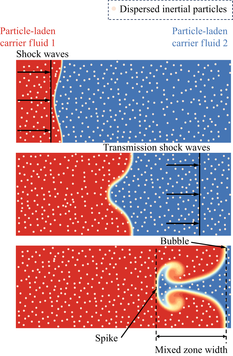
Before proceeding with detailed analysis, we outline the basic physical problem considered in this study. We focus on the instability development of multimedia fluid interface disturbances in particle-laden flows. This study investigates the influence of particles on the fluid interface evolution and provides a quantitative theoretical model. Within a certain range of particle loading, when the fluid interface is impacted by shock waves, baroclinic vorticity deposition occurs, inducing a phenomenon similar to single-phase RMI. Figure 1 shows a schematic diagram of the RMI phenomenon induced by the shock wave impact in a multimedia fluid under particle loading. In the evolution of particle-laden RMI interface instability, it also goes through a linear evolution stage and then enters a nonlinear evolution stage. Given the scarcity of research on the mechanism and theoretical models governing the nonlinear stage, the present study focuses on this nonlinear evolution stage. In the following theoretical modelling, we construct the multiphase potential flow theory within a coordinate system attached to the moving interface (see § 2.2), and then solve it to obtain the fingering model of the relative velocity evolution of the finger-like structure (see § 2.3). Subsequently, we construct the postshock interface velocity model of interface movement to further obtain the modelling of absolute velocity (see § 2.4). Finally, we provide a summary of these models (see § 2.5).

Figure 1.

Schematic diagram of fluid-interface instability evolution under particle loading.

2.2. Multiphase potential flow model

In this section, we introduce a multiphase potential flow theory for particle-laden RMI in large- $St$ systems at arbitrary density ratios. The model is formulated in two dimensions, consistent with common theoretical practice in RMI research, where two-dimensional frameworks often serve as the basis for analytical development (Zhou Reference Zhou2017a , Reference Zhoub ). We next outline the stages of RMI evolution and present the flow field characteristics of the nonlinear stage.

The temporal progression of RMI typically comprises an initial linear stage, followed by a nonlinear stage where complex interactions dominate. In the early stage of linear evolution, the shock wave is located closer to the disturbance interface, and the disturbance development at the interface is relatively small. At this stage, the compressibility of the flow field is crucial. The disturbance of the interface increases with time and enters a nonlinear evolution stage. In this stage, the shock wave has already moved away from the interface, and the pressure gradient in the flow field is small, which can be approximated as incompressible flow. At this stage, the amplitude of the interface disturbance is also quite significant, and the growth rate of the mixed zone width begins to increase nonlinearly.

The primary focus of our research is the nonlinear stage of the RMI within multiphase particle-laden flows. Given the considerable complexity inherent in multiphase dynamics, we have elected to exclude initial transient phenomena, specifically system startup and the initial compressible stages (cf. single-phase systems (Zhang et al. Reference Zhang, Deng and Guo2018; Li et al. Reference Li, Chen, Zhai and Luo2025)), to refine the focus of the investigation. Since the shock wave has already moved beyond the interface, it establishes conditions where the entire flow field can be effectively treated as incompressible. Consequently, we utilize the incompressible fluid governing equations for the theoretical derivation. Particle–particle collisions are neglected, and only drag is considered for particle–fluid interactions. Since existing potential flow models do not account for dense particle concentrations or strong interface–particle momentum coupling, we start from the compressible formulation of Tian et al. (Reference Tian, Zeng, Meng, Chen, Guo and Xue2020) and subsequently apply the incompressibility assumption. The resulting equations provide an effective description of the approximately incompressible, particle-laden, multiphase flow characteristic of the nonlinear RMI stages, and the governing equations can be given as

(2.1) \begin{align} \boldsymbol{\nabla }\boldsymbol{\cdot }\boldsymbol{u}_f=0, \end{align}

(2.2) \begin{align} \alpha _f\rho_{\!f}\frac {\mathrm{D}\boldsymbol{u}_f}{\mathrm{D}t}+\boldsymbol{\nabla }\left ( \alpha _fP \right ) =-P\boldsymbol{\nabla }\alpha _p+\frac {\alpha _p\kappa _p}{V_p}\left ( \boldsymbol{u}_p-\boldsymbol{u}_f \right ) , \end{align}

(2.3) \begin{align} \alpha _p+\alpha _f=1, \end{align}

where $\alpha _f$ , $\alpha _p$ are the fluid and particle volume fractions, $\rho_{\!f}$ is the fluid density, $\boldsymbol{u}_f$ is the fluid velocity, $\boldsymbol{u}_p$ is the particle velocity, $P$ is the pressure and $\kappa _p = 6\pi r_p\mu$ is the Stokes drag coefficient ( $r_p$ , particle radius; $\mu$ , dynamic viscosity). The momentum (2.2) includes: (i) gas momentum rate $\alpha _f\rho_{\!f}\mathrm{D}\boldsymbol{u}_f/\mathrm{D}t$ , (ii) pressure gradient force $\boldsymbol{\nabla }(\alpha _f P)$ , (iii) nozzling term $-P\boldsymbol{\nabla }\alpha _p$ (Baer & Nunziato Reference Baer and Nunziato1986), (iv) interphase drag $\alpha _p\kappa _p ( \boldsymbol{u}_p-\boldsymbol{u}_f ) /V_p$ , where $V_p = \pi d_p^3/6$ is the volume of a spherical particle ( $d_p$ , diameter). Here, the magnitude analysis of the fluid viscosity is detailed in Appendix B.1. Due to the fact that the Reynolds number of fluid flow ( $\textit{Re}_L$ ) is much higher than that of particles ( $\textit{Re}_p$ ), the magnitude of the viscosity of the fluid itself is extremely small, so it is negligible.

Figure 2.

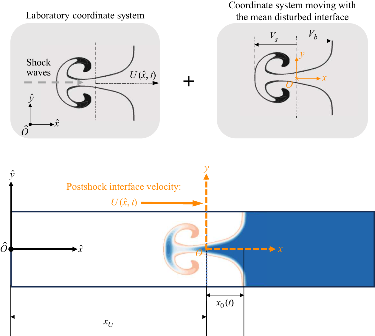
Schematic diagram of coordinate system: the laboratory coordinate system is illustrated as $( \hat {x},\hat {y} )$ , and the non-inertial work coordinate system that follows the mean disturbed interface movement is $( x,y )$ . The average interface velocity in the laboratory coordinate system is $U( \hat {x},t )$ .

We begin by introducing the reference frames employed in this study. The laboratory coordinate system we usually use in scientific research is an inertial frame and ground coordinate system as $ ( \hat {x},\hat {y} )$ . In the following theoretical derivation, we focus on the coordinate system $ ( {x},{y} )$ that follows the postshock fluid flow (see figure 2). We place the coordinate system at the moving interface, and the velocity at which this coordinate system moves is $U ( \hat {x},t )$ (see from the laboratory frame $ ( \hat {x},\hat {y} )$ ), which is called the postshock interface velocity. It is worth noting that, unlike single-phase systems, the postshock interface velocity is always constant ( ${\rm d}U ( \hat {x},t ) /{\rm d}t=0$ ) and the coordinate system $ ( {x},{y} )$ moving with the mean disturbed interface of single-phase systems is an inertial frame. However, in multiphase systems, the postshock interface velocity continuously decays over time ( ${\rm d}U ( \hat {x},t ) /{\rm d}t\ne 0$ ) and the coordinate system $ ( {x},{y} )$ moving with the mean disturbed interface is a non-inertial frame, as shown in § 2.4. To model the absolute velocity of spikes or bubbles, we first model their velocity relative to the mean interface within a relative reference frame $ ( {x},{y} )$ . The absolute velocity is then obtained by combining this relative velocity with the modelled postshock interface velocity.

Subsequently, we present the approximate conditions and physical justifications adopted for the theoretical derivation. The potential flow model is constructed under the following assumptions. First, the governing equation (2.2) neglects fluid–fluid viscosity but retains the fluid–particle viscosity. We couple the viscous shear stress and the pressure gradient force into the drag model. Second, we assume the particle-laden multiphase flow to be an irrotational potential flow in the fingertips of the fluid interface. At the large scale, the carrier fluid is assumed inviscid, and the particles are considered as point particles with no rotation of the particles relative to the fluid. Their particle-induced wake vortices are neglected, because both the spatial and temporal scales of wakes are much smaller than the characteristic scales of RMI evolution. The validity of irrotational potential flow assumptions is supported by numerical simulations (see Appendix A.1). The results show that, although vorticity is generated in particle-laden RMI, the dominant high-vorticity regions remain localized at the spike–bubble interface where baroclinic torque is deposited. The additional vorticity induced by particle shear is at least two orders of magnitude smaller than the baroclinic vorticity in the instability region. Therefore, it can be safely ignored.

Accordingly, we introduce velocity potential functions $\phi _1$ and $\phi _2$ for the two distinct fluid media on either side, with the corresponding velocity fields given by $\boldsymbol{u}_{f_1} = -\boldsymbol{\nabla }\phi _1, \boldsymbol{u}_{f_2} = -\boldsymbol{\nabla }\phi _2$ . Note that the potential function is also established on the coordinate system of the moving interface.

In studies on multiphase RMI, the Stokes number ( $St$ ) is defined as the ratio of particle relaxation time $t_p$ to the flow characteristic time $t_f$ , as $St=t_p/t_f$ . The particle relaxation time is given by $t_p=\rho _p d_p^2/(18\mu )$ based on Stokes’ drag law, where $\rho _p$ denotes the particle density, $d_p$ is the particle diameter and $\mu$ represents the dynamic viscosity of the carrier fluid. The characteristic time $t_f$ of flow is defined as the ratio of the wavelength $\lambda$ of interface disturbance to the velocity of interface motion accelerated by shock waves $U_{inf0}^{+}$ , as $t_f=\lambda /U_{inf0}^{+}$ . The specific expression for the $St$ number is as follows: $St=\rho _pU_{inf0}^{+}{d_p}^2/(18\mu \lambda)$ . A large $St$ value ( $St\gg 1$ ) signifies that particle velocity fails to equilibrate with the fluid velocity, approaching a frozen regime, as particle inertia dominates over fluid inertia. Therefore, we can assume that $|\boldsymbol{u}_p|/|\boldsymbol{u}_f|\ll 1$ .

In the following work, we adopt a coordinate system attached to the interface moving with the fluid. The momentum equation can be rewritten as adding the inertial force of the non-inertial frame:

(2.4) \begin{equation} \frac {\partial \boldsymbol{u}_{f_i}}{\partial t}+\frac {1}{2}\boldsymbol{\nabla }\left ( \boldsymbol{u}_{f_i}\boldsymbol{\cdot }\boldsymbol{u}_{f_i} \right ) -\boldsymbol{u}_{f_i}\times \left ( \boldsymbol{\nabla }\times \boldsymbol{u}_{f_i} \right ) =-\frac {1}{\rho _{f_i}}\left ( \boldsymbol{\nabla }\!P_i \right ) +\frac {\alpha _{p_i}\kappa _{p_i}}{\alpha _{f_i}\rho _{f_i}V_{p_i}}\boldsymbol{\nabla }\phi _i-\frac {\mathrm{d}U}{\mathrm{d}t}\boldsymbol{e}_x. \end{equation}

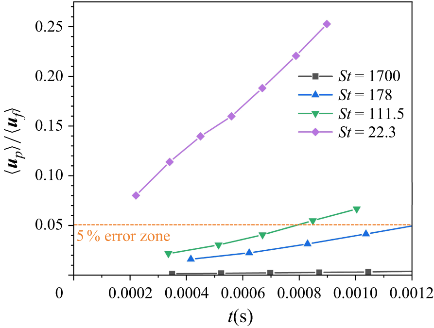
It is worth noting that we have transformed the drag force dominating the particle-laden flow system into a potential-mechanics form, which enables subsequent mathematical transformations. The threshold of the Stokes number is $St\gt 200$ . Within this regime, we adopt the simplified approximation $|\boldsymbol{u}_p|/|\boldsymbol{u}_f|\ll 1$ (see Appendix A.2 for details). The theoretical derivation range of $St$ numbers supported by numerical simulation is shown in the figure 11(c). Through mathematical transformations from (2.2) and (2.3), we can obtain

(2.5) \begin{equation} \frac {\partial \boldsymbol{u}_{f_i}}{\partial t}+\boldsymbol{\nabla }\left ( \frac {1}{2}\boldsymbol{u}_{f_i}\boldsymbol{\cdot }\boldsymbol{u}_{f_i}+\frac {P_i}{\rho _{f_i}}-s_i\phi _i+\frac {\mathrm{d}U}{\mathrm{d}t}x \right ) =2\boldsymbol{u}_{f_i}\times \boldsymbol{\omega }_{f_i}, \end{equation}

where we define the attenuation coefficient of each phase, $s_i=\alpha _{p_i}\kappa _{p_i}/(\alpha _{f_i}\rho _{f_i}V_{p_i})$ . Based on the irrotational assumption $\boldsymbol{\omega }_{f_i}=0$ of the flow field, we can obtain the equation for a certain fluid phase:

(2.6) \begin{equation} -\frac {\partial \phi _i}{\partial t}+\frac {1}{2}\left ( \boldsymbol{\nabla }\phi _i \right ) ^2+\frac {P_i}{\rho _{f_i}}-s_i\phi _i+\frac {\mathrm{d}U}{\mathrm{d}t}x=C_i\left ( t \right ). \end{equation}

Here $C_i ( t )$ is an arbitrary function that depends only on time $t$ . We subtract the (2.6) for each fluid term and introduce pressure and velocity equilibrium conditions ( $P_1=P_2, and\,\,\partial \phi _1/\partial x=\partial \phi _2/\partial x\,\, at\,\,x=\eta$ ). Consequently, the dynamic boundary conditions for two-phase flow are obtained

(2.7) \begin{align} \begin{split} -\rho _{f_1}\frac {\partial \phi _1}{\partial t} + \rho _{f_2}\frac {\partial \phi _2}{\partial t} + \frac {1}{2}\rho _{f_1}\left ( \boldsymbol{\nabla }\phi _1 \right ) ^2 - \frac {1}{2}\rho _{f_2}\left ( \boldsymbol{\nabla }\phi _2 \right ) ^2 \\[6pt] - s_1\phi _1\rho _{f_1} + s_2\phi _2\rho _{f_2} + \rho _{f_1}\frac {{\rm d}U_1}{{\rm d}t}\eta - \rho _{f_2}\frac {{\rm d}U_2}{{\rm d}t}\eta = f\left ( t \right ) , \quad \text{at} \ x = \eta . \end{split} \end{align}

Here, $x=\eta ( y,t )$ is the position of the interface in time, and $f ( t )$ denotes an arbitrary time-dependent function. The governing equations incorporate explicit four-way coupling between particles and the carrier fluid, comprehensively accounting for the interdependent effects of (i) interphase drag forces, (ii) phase-specific volume fractions ( $\alpha _p$ for particles, $\alpha _f$ for fluid), (iii) particle radius distribution $r_p$ , (iv) particle material density $\rho _p$ and (v) carrier fluid density $\rho_{\!f}$ . This formulation enables precise characterization of momentum exchange mechanisms critical to RMI evolution in dense particle-laden flows. Moreover, for kinematic boundary conditions, it is necessary to satisfy the interface preservation equation, which has the same form as the single-phase theory.

In conclusion, we obtain a potential flow model for particle-laden multiphase RMI. It contains two Laplace equations (2.8), two kinematic boundary conditions (2.9) and one dynamic boundary condition (2.10); the expression for the parameter $s_i$ used here is given in (2.11), all as follows:

(2.8) \begin{equation} {\nabla} ^2\phi _i\left ( t,x,y \right ) =0 \left ( i=1,2. \right ) , \end{equation}

(2.9) \begin{equation} \frac {\partial \eta }{\partial t}-\frac {\partial \phi _i}{\partial y}\frac {\partial \eta }{\partial y}+\frac {\partial \phi _i}{\partial x}=0\,at\,\,x=\eta \left ( i=1,2. \right ), \end{equation}

(2.10) \begin{align} \begin{split} -\rho _{f_1}\frac {\partial \phi _1}{\partial t} + \rho _{f_2}\frac {\partial \phi _2}{\partial t} + \frac {1}{2}\rho _{f_1}\left ( \boldsymbol{\nabla }\phi _1 \right ) ^2 - \frac {1}{2}\rho _{f_2}\left ( \boldsymbol{\nabla }\phi _2 \right ) ^2 \\[3pt] - s_1\phi _1\rho _{f_1} + s_2\phi _2\rho _{f_2} + \rho _{f_1}\frac {{\rm d}U_1}{{\rm d}t}\eta - \rho _{f_2}\frac {{\rm d}U_2}{{\rm d}t}\eta = f\left ( t \right ) , \quad \text{at} \ x = \eta , \end{split} \end{align}

(2.11) \begin{equation} s_i=\frac {\alpha _{p_i}\kappa _{p_i}}{\alpha _{f_i}\rho _{f_i}V_{p_i}}. \end{equation}

2.3. Universal fingering model

The potential theory framework for particle-laden multiphase flows, governed by (2.8)–(2.11), provides the foundation for constructing a universal fingering model. To construct the relative velocity of the finger-like structure, we solve it in a relative coordinate system. We employ the velocity potential function (2.12) into the multiphase potential theory based on experience from previous numerical simulations that incorporates Atwood number ( $A$ ) effects, which has been used in Zhang & Guo (Reference Zhang and Guo2016),

(2.12) \begin{align} \phi _i ( t,x,y) =a_i (t) \cos ( ky ) e^{ ( -1 ) ^ikx}+b_i ( t ) \cos ( c ( t ) ky ) e^{ ( -1 ) ^ic ( t ) kx}\,\, ( i=1,2.) \end{align}

where $c ( t )$ is a function concerning Atwood number ( $A$ ). Notably, while the velocity potential function is formally identical to that in Zhang & Guo (Reference Zhang and Guo2016), its parameters differ significantly between single-phase and multiphase conditions. Model formulations in multiphase studies inherently incorporate interphase coupling effects, including particle volume fraction, radius, density and associated descriptors. The coefficients, $a_i ( t )$ , $b_i ( t )$ , in the velocity potential function that evolve over time can describe the behaviour of RMI and the additional drag damping caused by the presence of particle phases. Explicitly, the functional dependencies of the parameters $a_i ( t )$ and $b_i ( t )$ are given as follows: $a_i ( t ) =f_i ( t,A,\alpha _p/\alpha _f,r_p,\mu _{f1},\mu _{f2},\rho _{f1},\rho _{f2} )$ , $b_i ( t ) =g_i ( t,A,\alpha _p/\alpha _f,r_p,\mu _{f1},\mu _{f2},\rho _{f1},\rho _{f2} )$ .

We employ the multiphase Atwood number derived from the particle–fluid velocity relaxation effects, which has the same form as the single-phase form. We define the Atwood number as $A= ( \rho _1-\rho _2 ) / ( \rho _1+\rho _2 )$ and $A\gt 0$ for bubbles and $A\lt 0$ for spikes. Note that in particle-laden systems, the selected Atwood numbers are multiphase Atwood numbers. Based on the research of Meng et al. (Reference Meng, Zeng, Tian, Zhou and Shen2019b), there are significant differences between Atwood numbers in the small $St$ systems (derived by equivalent density (see Ukai et al. Reference Ukai, Balakrishnan and Menon2010)) and the large $St$ system. In the large $St$ system, the RMI is driven only by the density difference of the gas-phase and is totally independent of particle density. Therefore, it remains consistent in form with single-phase situations.

The interface function of a spike or bubble is approximated as $\eta ( t,y ) =x_0 ( t ) +\xi ( t ) ky^2,$ due to its similarity in shape to a parabolic shape, where $x_0 ( t )$ and $\xi ( t )$ are the streamwise position and the curvature of the fingertip. We find this form is applicable to cases from single-phase to moderately dense particles. In the configuration, the curvature is always non-positive, i.e. $\xi \leqslant 0$ .

Subsequent sections detail the theoretical derivation through three key components: (i) perturbation analysis, (ii) quasisteady state postulation and (iii) velocity equation resolution yielding closed-form approximate solutions. The analysis first addresses (i) perturbation analysis by substitution into (2.9) with expansion to $y^2$ :

(2.13) \begin{equation} \frac {\mathrm{d}x_0\left ( t \right )}{\mathrm{d}t}+\left ( -1 \right ) ^ik\left ( a_ie^{\left ( -1 \right ) ^ikx_0}-cb_ie^{\left ( -1 \right ) ^ickx_0} \right ) \,\, =0, \end{equation}

(2.14) \begin{align} 2\frac {\mathrm{d}\xi \left ( t \right )}{\mathrm{d}t}+6\xi k^2\left ( a_ie^{\left ( -1 \right ) ^ikx_0}+c^2b_ie^{\left ( -1 \right ) ^ickx_0} \right ) -\left ( -1 \right ) ^ik^2\left ( a_ie^{\left ( -1 \right ) ^ikx_0}+b_ic^3e^{\left ( -1 \right ) ^ickx_0} \right ) =0.\\[-12pt]\nonumber \end{align}

Accordingly, the coefficients $a_1 ( t )$ , $b_1 ( t )$ , $a_2 ( t )$ , $b_2 ( t )$ are determined (see (C1)). Subsequently, we incorporate these coefficients into the dynamic boundary conditions (2.10) and perturb them to the quadratic term of $y$ . The second-order governing equation emerges as

(2.15) \begin{align} \begin{split} & F_1\!\left [16\!\left (\frac {\mathrm{d}\xi }{\mathrm{d}t}\right )^2 -10ckv\frac {\mathrm{d}\xi }{\mathrm{d}t}+c^2k^2v^2\right ] +2F_2\frac {\mathrm{d}\xi }{\mathrm{d}t}\frac {\mathrm{d}c}{\mathrm{d}t} +F_3kv\frac {\mathrm{d}c}{\mathrm{d}t}\\ &\quad +F_4\Bigl [2F_4kA\frac {\mathrm{d}U}{\mathrm{d}t}\xi -2F_5\frac {{d}^2\xi }{\mathrm{d}t^2} +F_6k\frac {\mathrm{d}v}{\mathrm{d}t}\Bigr ]\\ &\quad +F_4k\Bigl [(c^2+c)\hat {S}-\xi (36\xi ^2-1)\mathcal{E} +c^2\xi \mathcal{E}-c\xi \mathcal{E}\Bigr ]v\\ &\quad -2F_4\Bigl [(c+1)\hat {S}-3\xi \mathcal{E}\Bigr ] \frac {\mathrm{d}\xi }{\mathrm{d}t}=0, \end{split} \end{align}

where the terms $\hat {S}$ , $\mathcal{E}$ are

(2.16) \begin{align} \hat {S} = \frac {\rho _1 s_1 + \rho _2 s_2}{\rho _1 + \rho _2} = \frac {\alpha _p 6\pi r_p (\mu _{f_1} + \mu _{f_2})}{\alpha _f V_p (\rho _1 + \rho _2)}, \quad \mathcal{E} = \frac {s_1 \rho _1 - s_2 \rho _2}{\rho _1 + \rho _2} = \frac {\alpha _p 6\pi r_p (\mu _{f_1} - \mu _{f_2})}{\alpha _f V_p (\rho _1 + \rho _2)}. \end{align}

In (2.15), $v=\mathrm{d}x_0/\mathrm{d}t$ is the velocity of the fingertip. The coefficients $F_i$ are listed in Appendix C (C2).

Secondly, the derivation then progresses to (ii) quasisteady state postulation. From the quasisteady state stage, the curvature of the fingertip is insensitive to time in this stage (Glimm, Li & Lin Reference Glimm, Li and Lin2002; Sohn Reference Sohn2004), namely, $\mathrm{d}\xi /\mathrm{d}t=0$ , and $\mathrm{d}c/\mathrm{d}t=0$ . The equation can be simplified as (2.17). The curvature evolution occurs much faster than the interface growth rate, leading to a quasisteady curvature state shortly after flow field initiation,

(2.17) \begin{align} \begin{split} &F_1 c^{2}k^{2}v^{2} +F_4\!\left (2F_4kA\frac {\mathrm{d}U}{\mathrm{d}t}\xi +F_6k\frac {\mathrm{d}v}{\mathrm{d}t}\right )\\ &\quad +F_4k\Bigl [(c^{2}+c)\hat {S}-\xi (36\xi ^{2}-1)\mathcal{E} +c^{2}\xi \mathcal{E}-c\xi \mathcal{E}\Bigr ]v =0. \end{split} \end{align}

We introduce the parameters $\alpha$ , $\beta$ and $\varUpsilon$ as follows:

(2.18a) \begin{align} \alpha &=\frac {F_{1}}{F_{4}F_{6}}\,c^{2}, \end{align}

(2.18b) \begin{align} \beta &=\frac {(c^{2}+c)\hat {S}-\xi (36\xi ^{2}-1)\mathcal{E} +c^{2}\xi \mathcal{E}-c\xi \mathcal{E}}{F_{6}}, \end{align}

(2.18c) \begin{align} \varUpsilon &=\frac {2F_{4}A\xi }{F_{6}}. \end{align}

Therefore, we can obtain the simplified velocity (2.19). Also we have $\mathrm{d}U/\mathrm{d}t\lt 0$ , $\varUpsilon \lt 0$ ,

(2.19) \begin{align} \begin{split} \alpha kv^2+\varUpsilon \frac {\mathrm{d}U}{\mathrm{d}t}+\frac {\mathrm{d}v}{\mathrm{d}t}+\beta v=0. \end{split} \end{align}

Based on numerical experiments, we find that spikes and bubbles in multiphase RMI have similar finger-like structures and curvature characteristics as single-phase within regimes of moderate particle volume fractions ( $\alpha _p\lt 0.2$ ) (see § 4.1 and figure 12 for details). To capture multistage dynamics, we note that the short-term behaviour of the leading order is governed by the initial condition $v_0$ . Constructing a matched asymptotic solution bridging the initial transient phase and the quasisteady state requires adopting the approximations $\xi ( t ) \equiv \xi _{qs}$ and $c ( t ) \equiv -6\xi _{qs}$ (Zhang & Guo Reference Zhang and Guo2016). We conclude the relationship between the curvature and Atwood number in the quasisteady state stage as

(2.20) \begin{align} c_{qs}/\xi _{qs}=-6+O(1), \xi _{qs}(A)&=-\left ( 3+A \right ) /\left ( 12\sqrt {2(1+A)} \right ),\nonumber\\[3pt] &\quad c_{qs}(A)=\left ( 3+A \right ) /\left(2\sqrt {2(1+A)}\right). \end{align}

The derivation completes with (iii) velocity equation resolution, yielding closed-form approximate solutions. The governing equation for velocity is as follows:

(2.21) \begin{equation} \mathrm{d}v/\mathrm{d}t=-\alpha kv^2-\beta v-\varUpsilon \frac {\mathrm{d}U}{\mathrm{d}t}, \end{equation}

where the coefficients $\alpha$ , $\beta$ , $\varUpsilon$ are defined as

(2.22) \begin{equation} \alpha = \frac {F_1}{F_4 F_6}c^2 = \frac {3(1{+}A)(3{+}A)\left [4(3{+}A) + \sqrt {2}(9{+}A)(1{+}A)^{1/2}\right ]}{4\left [3{+}A + \sqrt {2}(1{+}A)^{1/2}\right ]\left [(3{+}A)^2 + 2\sqrt {2}(3{-}A)(1{+}A)^{1/2}\right ]}, \end{equation}

(2.23) \begin{equation} \beta = \frac {(c^2{+}c)\hat {S} - \xi (36\xi ^2{-}1)\mathcal{E} + c^2\xi \mathcal{E} - c\xi \mathcal{E}}{c^2{+}c + 2A\xi (c^2{-}c{+}1) - 72A\xi ^3} = \frac {-2\sqrt {A{+}1}\left [6\left (\varGamma _1\hat {S}\right ) + \left (\varGamma _2\mathcal{E}\right )\right ]}{\mathcal{D}}, \end{equation}

(2.24) \begin{equation} \varUpsilon =\frac {2F_4A\xi }{F_6}=-\frac {2A\left ( A+3+\sqrt {2A+2} \right )}{(A+3)^2+2(3-A)\sqrt {2A+2}}, \end{equation}

with $\varGamma _1 = A(\sqrt {A{+}1}{+}2\sqrt {2}) + 3\sqrt {A{+}1}{+}2\sqrt {2}$ , $\varGamma _2 = A(\sqrt {A{+}1}{-}2\sqrt {2}) + 3\sqrt {A{+}1}{-}2\sqrt {2}$ and denominator $\mathcal{D}$ as given in the original expression. Equation (2.21) has a numerical solution. For a more intuitive discussion of the results, we have chosen the approximate analytical solution as

(2.25) \begin{align} \begin{split} V_{b/s}\approx \underbrace {\frac {v_0}{e^{\beta t}+\alpha kv_0\left ( \frac {1-e^{\beta t}}{-\beta } \right )}}_{(\mathrm{I) Particle}-\mathrm{fluid}\ \mathrm{coupling}\ \mathrm{drag}\ \mathrm{effect}\ \mathrm{term}}+\underbrace {\varUpsilon \left ( U_0-U\left ( t \right ) \right ) }_{(\mathrm{II) Postshock}\ \mathrm{interface}\ \mathrm{velocity} \ \mathrm{inertial}\ \mathrm{force}\ \mathrm{term}}, \end{split} \end{align}

where $V_{b/s}$ is the bubbles/spikes velocity relative to the interface, $v_0$ is the initial velocity of the nonlinear stage. Here $U_0$ is the initial velocity of the postshock interface; $U ( t )$ is the functional expression of the postshock interface velocity over time. In conclusion, this yields an approximate solution for the relative velocity’s evolution of finger-like structures. The solution consists of two components: (I) interphase drag coupling between particles and fluid, (II) non-inertial frame effects induced by the postshock interface velocity $U(t)$ field. To account for postshock interface velocity effects and derive governing equations for the absolute velocity of finger-like structures, § 2.4 details the postshock interface velocity model and analyses its impact on RMI dynamics.

2.4. Postshock interface velocity attenuation model

In the derivation of the previous section, we obtain the relative velocity of the finger-like structure with respect to the postshock interface velocity. This section establishes a model for the postshock interface velocity evolution of the multiphase RMI system to examine the effect of the inertial force term on the spike and bubble amplitude growth.

In single-phase RMI studies, the postshock interface velocity is unattenuated and conventionally modelled as constant. In research, this constant is often chosen as the postshock accelerated velocity of the mean multiple media interface $\Delta U$ (Jacobs & Sheeley Reference Jacobs and Sheeley1996; Zhang & Sohn Reference Zhang and Sohn1996; Mikaelian Reference Mikaelian1998) and often measured directly through undisturbed interface settings or calculated using empirical formulae. However, in dense particle-laden multiphase systems, postshock interface velocity is no longer constant, especially exhibiting significant attenuation effects. Prior models of RMI growth rates that use relative coordinate systems often neglect postshock interface velocity effects. This omission can lead to significant errors in the context of dense particle-laden flows. Previous approaches of single-phase systems lack interphase energy transfer terms and necessitate modification to accurately model multiphase RMI fingering evolution. The interphase momentum coupling in gas–particle systems also alters RMI dynamics by modifying the mean interface velocity field. Particle-laden flows introduce dissipation mechanisms absent in single-phase RMI: as shocks accelerate the multiphase interface, momentum transfer to particles via drag forces decays both the postshock mean interface velocity and the relative motion of spikes and bubbles.

The redistribution of momentum between the particle and fluid phases critically governs the evolution of multiphase RMI, necessitating accurate postshock mean interface velocity decay modelling. The rationale for avoiding direct application of potential flow theory in the laboratory coordinate system to solve for postshock interface velocity is twofold: under particle-laden conditions – particularly with dense loading – the flow field exhibits complex wave interactions, including transmitted and reflected shock waves resulting from shock-particle cloud interactions (Osnes et al. Reference Osnes, Vartdal, Omang and Reif2020; Boniou & Fox Reference Boniou and Fox2023). Furthermore, unlike single-phase scenarios where pressure gradients become negligible after the primary shock passage, the presence of particles may introduce significant pressure gradients throughout the flow field. All of these increase the complexity of the integrated solution, and due to the fact that the magnitude of the postshock interface velocity is 10 times that of the spike/bubble velocity, deviations in the postshock interface velocity can lead to inaccurate absolute velocity modelling results.

For quasi-one-dimensional flow, the postshocked interface velocity attenuation model can be derived from (2.1)–(2.3), yielding the reduced streamwise momentum equation,

(2.26) \begin{equation} \frac {{\rm d}U\left ( t \right )}{{\rm d}t} = -\frac {1}{\rho_{\!f}} \frac {\partial P_{\!f}}{\partial x} - s U\left ( t \right ), \end{equation}

where $ U(t)$ is the mean streamwise interface velocity, $ s = \alpha _p \kappa _p / (V_p \alpha _f \rho_{\!f})$ is the drag coupling coefficient, and the particle velocity is approximated as $ u_{px} \approx 0$ for large Stokes numbers ( $ St \gg 1$ ). Immediately after the shock passage, the interface velocity undergoes a sharp increment to $U_0$ . Its subsequent temporal evolution is determined by the competition between the pressure gradient force ( $F_p=-\partial P_{\!f}/\partial x$ ) and the particle drag ( $F_d=\alpha _p\kappa _p ( \boldsymbol{u}_p-\boldsymbol{u}_f ) /V_p$ ). 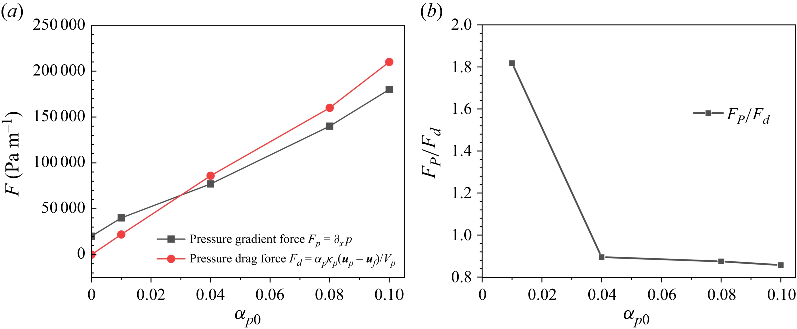However, directly modelling the pressure-gradient term $-\partial P_{\!f}/\partial x$ under dense particle loading is challenging, since inertial particles significantly alter the wave dynamics, leading to a complex, multiscale relaxation process not amenable to simple closure. Numerical simulations show that, unlike in the single-phase case, the pressure-gradient force is comparable in magnitude to the particle drag and often acts in opposition, moderating the net deceleration rate. For particle volume fractions in the range 0.04–0.1, the ratio $\mid \partial _xP\mid /\mid F_d\mid \approx O(1)$ remains approximately 0.8–0.9 (see figure 4), indicating that the pressure-gradient force scales nearly linearly with the drag. Therefore, we can assume that $-( {1}/{\rho })\partial _x P = s_p F_d$ , where $s_p$ is a constant related to the pressure gradient. Therefore, it can be inferred that the average interface velocity has the following form: ${\rm d}U/{\rm d}t=- (s-s{\times}s_p )U$ . To circumvent the difficulty of theoretical modelling while capturing the net effect, we introduce an effective attenuation coefficient, $ \varXi$ , which encapsulates the combined contributions of the particle drag, the particle-modified pressure gradient and their nonlinear interplay. This leads to a closed-form attenuation model for the interface mean velocity,

(2.27) \begin{equation} U\left ( t \right ) = U_{0} e^{-\varXi t}, \end{equation}

where time $ t=0$ is defined as the instant the shock traverses the interface. For single-phase RMI ( $ \alpha _p = 0$ ), we have $ \varXi \approx 0$ , and the model reduces to a constant velocity $ U(t) = U_0$ , consistent with the classical impulsive acceleration model where postshock pressure gradients are indeed negligible. The initial velocity $ U_0$ depends on standard shock–interface parameters (fluid densities, shock strength), while the effective coefficient $ \varXi$ additionally encodes the effects of particle loading ( $ \alpha _p$ ) and inertia ( $ St$ ). The schematic diagram of the postshock interface velocity coordinate system for $U(t)$ is shown in figure 2.

The exponential-decay ansatz adopted here is consistent with the approximate form used by Marble (Reference Marble1970) to describe the evolution of physical quantities in the non-equilibrium relaxation zone of postshock dusty-gas flows. The attenuation rate $ \varXi$ can be quantified by fitting the interface velocity attenuation curve, usually using a reference case without initial disturbance for scaling, as shown in table 1. Figure 3 shows the initial conditions for a given plane interface of a multimedia fluid (undisturbed). Figure 5 shows the results of the numerical simulation of postshock interface velocity. For an introduction to numerical algorithms, please refer to § 3.1. It can be observed (see figure 5 a) that within the range where the initial volume fraction of particles is relatively low ( $\alpha _{p0}\lt 0.01$ ), the effect of postshock interface velocity attenuation due to particle blockage is relatively small; but when the particle volume fraction is greater than $\alpha _{p0}\gt 0.04$ , there is already a significant difference; when the initial volume fraction of particles is greater than $\alpha _{p0}\gt 0.1$ , the attenuation effect is very significant. The semiempirical expression we derived follows an exponential decay rate. Numerical simulation results versus the semiempirical model fit, as shown in figure 5(b), confirm this conclusion. We not only determined the decay coefficients for all simulation cases but also employed a logarithmic scale ( $\ln$ ) on the y-axis. As evident in figure 5(b), the cases exhibit clear linear trends, corroborating the exponential semiempirical model.

Table 1.

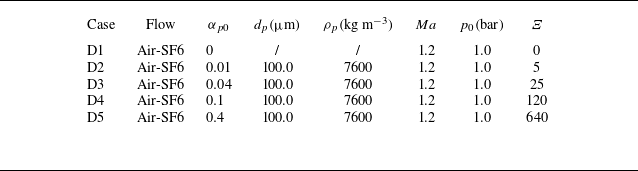
Case settings for postshock interface velocity attenuation test. Here, $\alpha _{p0}$ is the initial particle volume fraction, $\rho _p$ is the density of particles, $p_0$ is the preshock background pressure, $\varXi$ is the fitted coefficient and the preshock temperature is 298 K. The magnitude of $\textit{Re}_p$ is approximately $300- 1500$ and $St\sim 1700$ .

Building on the preceding section, we now examine how incorporating postshock interface velocity in the relative coordinate framework affects the modelling of spikes or bubbles’ growth rates in RMI. We perform a Taylor expansion of the approximate solution (2.25) obtained in the preceding section about $t=0$ to quantify deviations induced by the decay term and its coefficient,

(2.28) \begin{align} \begin{split} V_{b/s}\approx \frac {v_0}{e^{\beta t}+\alpha kv_0\left ( \frac {1-e^{\beta t}}{-\beta } \right )}+\varUpsilon \left ( U_0-U_0e^{-\varXi t} \right ) \sim \frac {v_0}{e^{\beta t}+\alpha kv_0\left ( \frac {1-e^{\beta t}}{-\beta } \right )}+U_0\varUpsilon \varXi t. \end{split} \end{align}

We further discuss the impact of inertial forces. We perform an order-of-magnitude analysis of key parameters. The characteristic time scale for RMI development is $t_{\textit{RMI}} \sim 10^{-3}\,\mathrm{s}$ . The parameter $\varXi$ , which has units of $\mathrm{s}^{-1}$ , spans values from $0$ to $10^{3}\,\mathrm{s}^{-1}$ . The dimensionless parameter $\varUpsilon$ scales as $O(10^{-1})$ , while the initial velocity magnitude is $U_0 \sim O(10^{2}\,\mathrm{m\,s}^{-1})$ . The characteristic velocity scale $V_{b/s}$ of our target system is $O(10^{1}\,\mathrm{m\,s}^{-1})$ . From this magnitude analysis, we deduce that the inertial forces arising from postshock interface velocity decay remain negligible when $\varXi$ is of the order of $10^{2}\,\mathrm{s}^{-1}$ or lower. However, when $\varXi$ reaches magnitudes of $10^{3}\,\mathrm{s}^{-1}$ and beyond, its suppressive effect on the spikes or bubbles growth rate in RMI becomes profoundly significant. Consequently, when the attenuation coefficient of the postshock interface velocity $U ( t )$ is small ( $\alpha _{p0}\lt 0.1$ ), the solution can be further approximated as

(2.29) \begin{equation} V_{b/s}\approx \frac {v_0}{e^{\beta t}+\alpha kv_0\left ( \frac {1-e^{\beta t}}{-\beta } \right )}. \end{equation}

The evolution of the RMI perturbation amplitude is primarily driven by the velocity difference between its spikes and bubbles within their relative coordinate system. Under conditions of extremely dense particle loading, the RMI undergoes freezing, leading to the cessation of its evolution (see § 4.1.3). This phenomenon can be explained by considering the relative coordinate framework: highly concentrated particle loading induces substantial inertial forces, which in turn suppress the development of the RMI. As in Case D5, the magnitude of the $\varXi$ coefficient is close to the $10^{3}\,\mathrm{s}^{-1}$ , and the attenuation term of the inertial force is very significant. At this point, the particles are extremely densely distributed in the flow field, and RMI is suppressed and eventually frozen (quenched) and typical finger-like structures such as spikes and bubbles in RMI evolution are no longer produced.

Figure 3.

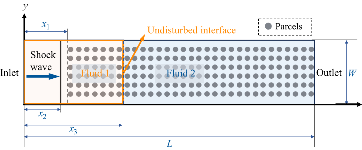
Schematic diagram of numerical simulation example set-up, with multimedia interface being an undisturbed plane. The circle represents a schematic diagram of the parcels carrying particles. Except for the initial multiphase interface without disturbance, all other settings can be found in § 3.2.

2.5. Model analysis and conclusions

In this section, we summarize and discuss the theoretical model proposed above. We obtain a theoretical model for multiphase RMI instability that differs from single-phase RMI systems. For particle-laden multiphase RMI systems, the loaded particles are within a certain range (large $St$ number system $St\gt 200$ , medium dense particle-laden $\alpha _{p0}\lt 0.1$ ), we introduce the unified fingering velocity theoretical model,

(2.30) \begin{align} \begin{aligned} u_{\textit{RM}}=\frac {1}{1+\tau _{\textit{RM}}},\quad {\rm with}\,\,u_{\textit{RM}}=\frac {v}{v_0},\quad\tau _{\textit{RM}}=\left ( \alpha kv_0+\beta \right ) \left ( \frac {1-e^{\beta t}}{-\beta } \right ) , \end{aligned} \end{align}

(2.31) \begin{equation} v=\left \{ \begin{array}{c} V\prime _b-U_{0}e^{-\varXi t},\quad \textit{for bubbles}\\ U_{0}e^{-\varXi t}-V\prime _s,\quad \textit{for spikes}\\ \end{array} \right ., \end{equation}

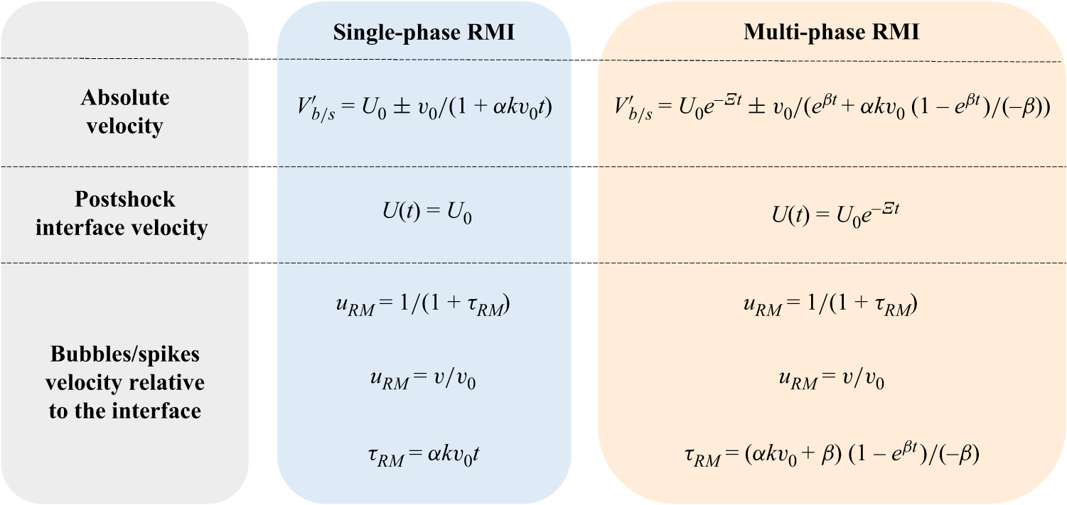
where $V\prime _s$ and $V\prime _b$ are, respectively, the absolute velocity of spikes and bubbles. The $u_{\textit{RM}}$ and $\tau _{\textit{RM}}$ are normalized velocity and time scale. Here $v_0$ is the initial velocity of the nonlinear stage, $v$ is the velocity of finger structures, $\alpha$ and $\beta$ govern instability growth and damping rates and $k$ is the wavenumber. Accordingly, the normalization framework of velocity evolution collapses to a universal scaling law. Figure 6 shows a schematic comparison of theoretical models for single-phase and multiphase RMI evolution.

Equation (2.30) degrades to the particle-free form $\tau _{\textit{RM}}=\alpha kv_0t$ , matching the form presented by Zhang & Guo (Reference Zhang and Guo2016), when the volume fraction of particles is relatively small, leading to coefficients $\varXi \approx 0$ and $\beta \approx 0$ , and the fingering velocity model degenerates as

(2.32) \begin{align} \begin{aligned} u_{\textit{RM}}=\frac {1}{1+\tau _{\textit{RM}}},\,\,{\rm with}\,\,u_{\textit{RM}}=\frac {v}{v_0},\,\,\tau _{\textit{RM}}=\alpha kv_0t \,\,{\rm and}\ v=\left \{ \begin{array}{c} V\prime _b-U_{0},\quad \textit{for bubbles}\\ U_{0}-V\prime _s,\quad \textit{for spikes}\\ \end{array} \right. . \end{aligned} \end{align}

The dimensionless time $\tau _{\textit{RM}}= ( \alpha kv_0+\beta ) ( 1-e^{\beta t} ) / ( -\beta )$ shows the nonlinear mapping effect of the particle effect on the time-dependent terms of RMI development. For the non-particle form $\tau _{\textit{RM}}=\alpha kv_0t$ , time exhibits a linear mapping relationship in its dimensionless form. However, in particle-laden flows, the characteristic time scale becomes $\alpha kv_0+\beta$ , which is greater than $\alpha kv_0$ . Additionally, a temporal modulation term of the form $ (1 - e^{-\beta t} )/(-\beta )$ emerges. This term introduces additional dynamic complexity into the evolution of RMI.

By modelling the growth rate $v_h$ ( $v_h= V_b-V_s$ ) of mixed zone width $h$ , we obtain the equation

(2.33) \begin{align} h=h_0+\left \{ \frac {1}{\alpha k}\ln \left ( 1+\frac {\alpha kv_0}{\beta }\left ( 1-e^{-\beta t} \right ) \right ) \right \} _b+\left \{ \frac {1}{\alpha k}\ln \left ( 1+\frac {\alpha kv_0}{\beta }\left ( 1-e^{-\beta t} \right ) \right ) \right \} _s , \end{align}

where $\left \{ \right \} _b$ and $\left \{ \right \} _s$ , respectively, indicate that all coefficients in parentheses are related to bubbles or spikes.

Based on the velocity expression of the finger-like structure in (2.21), there are three key influencing parameters. We further discuss and analyse these parameters: $\alpha$ represents the intrinsic instability-growth coefficient of RMI, $\beta$ represents the damping coefficient associated with the particle phase and $\varUpsilon$ represents the parameter characterizing the inhibitory effect of inertial force on the RMI growth rate. The evolution of RMI primarily depends on the retarding effect of Stokes drag and the work associated with both the intrinsic RMI dynamic pressure and inertial force, highlighting the interplay among these three factors in driving instability development. Note that $\beta$ and $\varUpsilon$ , which govern particle effects, are key factors controlling the development of particle-laden multiphase RMI and distinguish it from single-phase RMI. In § 2.4, we find that for medium-dense particle-laden flow ( $\alpha _{p0}\lt 0.1$ ), the influence of inertial force is relatively small and can be ignored.

Figure 4.

(a) The magnitude of pressure gradient force and drag force at different particle volume fractions. (b) The ratio of pressure gradient force to drag force at different particle volume fractions.

Figure 5.

(a) The result graph of postshock interface velocity changing with time under undisturbed initial interface settings as in figure 3. (b) Numerical simulation results versus the semiempirical model fit. The y-axis is plotted on a logarithmic scale ( $\ln$ ).

The damping attenuation term $\beta$ in theoretical modelling is mainly related to the particle-to-fluid volume fraction ratio, the densities and viscosities of the two carrier fluids and the particle diameter. Particle-induced suppression of RMI is governed by two drag-related parameters: the mean dynamic viscosity $\hat {S}$ and its differential component $\mathcal{E}$ . Theoretical analysis identifies $\hat {S}$ as the primary suppression mechanism, with $\mathcal{E}$ playing a secondary role. Increased $\hat {S}$ and $\mathcal{E}$ enhance viscous damping, attenuating fluid velocity and instability growth. Higher particle volume fraction ( $\alpha _p$ ) and smaller diameter ( $d_p$ ) further amplify flow attenuation, suppressing the growth rate of the disturbance amplitude. This attenuation is primarily governed by the momentum exchange between the phases. Physically, $\hat {S}$ quantifies the drag force exerted by the particles on a unit mass of fluid. The stronger attenuation effect of smaller particles stems from their larger surface area-to-volume ratio ( $A_p/V_p \propto 1/d_p$ ): at fixed $\alpha _p$ , reducing $d_p$ increases both the specific surface area ( $A_{sp} = 6\alpha _p/d_p$ ) and the particle number density ( $n \propto 1/d_p^3$ ), yielding $\hat {S} \propto \alpha _p/d_p^2$ and thus stronger attenuation.

Figure 6.

Comparison diagram of theoretical models for single-phase and multiphase RMI evolution, where the single-phase theory is taken from Zhang & Guo (Reference Zhang and Guo2016).

3.1. Numerical algorithm

The numerical simulations in this study were performed using the CMP-PIC method (Tian et al. Reference Tian, Zeng, Meng, Chen, Guo and Xue2020). As an improved Eulerian–Lagrangian approach, it is well-suited for simulating gas–particle systems across a wide range of flow regimes, including dilute, dense and granular flows. This method treats the gas as a continuous phase and tracks the dispersed particles in Lagrangian coordinates based on the particle-in-cell method, which can describe the motion of individual particles and the interaction between particles in detail. The gas-phase governing equations are discretized on a uniform Eulerian grid, while the parcels (containing particles) are tracked in the Lagrangian framework. It should be noted that even if the particle phase is incompressible except for the collision process, the gas–particle mixture as a whole is a compressible flow. The governing equations for the particle and gas phases are as follows.

3.1.1. Particle phase equations

Firstly, we introduce the governing equations and mechanical model of the particle phase. Newton’s second law of motion is applied to each particle separately, thus establishing the governing equations for the particle phase, as shown in (3.1) and (3.2). The mechanical model of particles is still an open problem in the study of multiphase RMI with shock–wave interactions in particle-laden flows. At this stage, three types of forces acting on particles are considered. The presence of shock waves makes the drag force $\boldsymbol{F}_{\textit{drag}}=\kappa _{p,i} ( \bar {\boldsymbol{u}}_f-\boldsymbol{v}_{p,i} ) /V_{p,i}$ and the pressure-gradient force $\boldsymbol{F}_{pgf}=-\boldsymbol{\nabla }\!P_{\!f}$ essential. In addition, for dense flows, collisions between particles cannot be ignored, so the collision force $\boldsymbol{F}_{\textit{col}}=-\rho _p\boldsymbol{A}_{p,i}$ must also be considered. Analysis of other forces, such as virtual mass, Basset history and Magnus forces, can be found in Appendix B.2. In these equations, subscripts $p$ and $f$ correspond to the particle and gas phases, respectively, and the subscript $i$ denotes the index of the particle package. Here $\boldsymbol{x}_{p,i}$ , $\boldsymbol{v}_{p,i}$ and $V_{p,i}$ , respectively, represent the position vector, velocity vector and volume of particle package $i$ . Here $\rho _p$ is the density of the particle phase; $\rho_{\!f}$ and $P_{\!f}$ represent the density and pressure of the gas, respectively, and $\bar {\boldsymbol{u}}_f$ denotes the average gas-phase velocity vector within the grid cell. Here $\alpha _f$ and $\alpha _p$ are the volume fractions of the gas and particle phases, respectively,

(3.1) \begin{align} \frac {\mathrm{d}\boldsymbol{x}_{p,i}}{\mathrm{d}t}=\boldsymbol{v}_{p,i}, \end{align}

(3.2) \begin{align} \rho _p\frac {\mathrm{d}\boldsymbol{v}_{p,i}}{\mathrm{d}t}=\boldsymbol{F}_{\textit{drag}}+\boldsymbol{F}_{pgf}+\boldsymbol{F}_{\textit{col}}. \end{align}

To account for the drag effect in particle–fluid coupling, this study adopted the Stokes drag model, where $\kappa _{p,i}$ is the drag coefficient of the particle package. It can be expressed as $\kappa _{p,i}=6\pi r_p\mu$ , where $r_p$ is the particle radius and $\mu$ is the fluid dynamic viscosity coefficient. To account for particle collisions, this study used the discrete element method (Alobaid & Epple Reference Alobaid and Epple2013), treating the collision process as the coupling effect of springs and dampers. Here $\boldsymbol{A}_{p,i}$ represents the collision contribution within particle package $i$ (see (3.3)). Here, $m_p$ is the mass of the particle package, $\delta _n$ represents the overlap length between two packages during collision and $k_{n,pc}$ , $\gamma _{n,pc}$ and $e_{pc}$ are the stiffness, damping and recovery coefficient of the package (see (3.4)),

(3.3) \begin{equation} \boldsymbol{A}_{p,i}=\frac {1}{m_p}\sum \nolimits _j^{}{\boldsymbol{F}_{ij,n}},\boldsymbol{F}_{ij,n}=k_{n,pc}\delta _n\boldsymbol{n}-\gamma _{n,pc}\boldsymbol{v}_{r,n}, \end{equation}

(3.4) \begin{equation} \gamma _{n,pc}=-\frac {2\ln e_{pc}}{\sqrt {\pi ^2+ \ln e_{pc}}}\sqrt {m_{pc}k_{n,pc}}. \end{equation}

3.1.2. Gas phase equations

Secondly, we introduce the governing equations for the gas phase. In the governing equations for the gas phase, we neglected the viscous effect of the fluid. To account for the two-way coupling between the gas and particle phases and the drag effect of particles on the fluid, the interaction viscosity is incorporated into the drag coefficient in the drag model. The two-way coupling between gas and particles is achieved through the source terms in the momentum and energy equations. The gas-phase governing equations are given in (3.5)–(3.9). Here, $\alpha _f$ represents the volume fraction of the gas phase (including fluid phases 1 and 2), $\beta _1$ represents the volume fraction of gas phase 1 in the total gas phase, $u_{fx}$ , $u_{fy}$ and $u_{fz}$ are the gas-phase velocities in the $x$ , $y$ and $z$ directions, and $\bar {u}_{fx}$ , $\bar {u}_{fy}$ and $\bar {u}_{fz}$ represent the average gas-phase velocity fields in the $x$ , $y$ and $z$ directions within the grid cell. Here $P_{\!f}\boldsymbol{\nabla }\alpha _p$ is the nozzling term. In addition, the volume fractions of the gas and particle phases must satisfy $\alpha _p+\alpha _f=1$ :

(3.5) \begin{equation} \frac {\partial \boldsymbol{U}}{\partial t}+\frac {\partial \boldsymbol{F}}{\partial x}+\frac {\partial \boldsymbol{G}}{\partial y}+\frac {\partial \boldsymbol{H}}{\partial z}=\boldsymbol{D}_p, \end{equation}

(3.6) \begin{equation} \frac {\partial \beta _1}{\partial t}+u_{fx}\frac {\partial \beta _1}{\partial x}+u_{fy}\frac {\partial \beta _1}{\partial y}+u_{fz}\frac {\partial \beta _1}{\partial z}=0, \end{equation}

(3.7) \begin{equation} \boldsymbol{U}=\!\left (\begin{array}{l} \alpha _f\rho_{\!f}\\ \alpha _f\beta _1\rho _{f1}\\ \alpha _f\rho_{\!f}u_{fx}\\ \alpha _f\rho_{\!f}u_{fy}\\ \alpha _f\rho_{\!f}u_{fz}\\ \alpha _f\rho_{\!f}E_f\\\end{array} \!\right)\!, \boldsymbol{F}=\!\left (\begin{array}{l} \alpha _f\rho_{\!f}u_{fx}\\ \alpha _f\beta _1\rho _{f1}u_{fx}\\ \alpha _f\rho_{\!f}u_{fx}u_{fx}+\alpha _fP_{\!f}\\ \alpha _f\rho_{\!f}u_{fy}u_{fx}\\ \alpha _f\rho_{\!f}u_{fz}u_{fx}\\ \alpha _f\rho_{\!f}E_fu_{fx}+\alpha _fP_{\!f}u_{fx}\\\end{array} \!\right)\!, \boldsymbol{G}=\!\left (\begin{array}{l} \alpha _f\rho_{\!f}u_{fy}\\ \alpha _f\beta _1\rho _{f1}u_{fy}\\ \alpha _f\rho_{\!f}u_{fx}u_{fy}\\ \alpha _f\rho_{\!f}u_{fy}u_{fy}+\alpha _fP_{\!f}\\ \alpha _f\rho_{\!f}u_{fz}u_{fy}\\ \alpha _f\rho_{\!f}E_fu_{fy}+\alpha _fP_{\!f}u_{fy}\\\end{array} \!\right)\!, \end{equation}

(3.8) \begin{equation} \boldsymbol{H}=\left ( \begin{array}{l} \alpha _f\rho_{\!f}u_{fz}\\ \alpha _f\beta _1\rho _{f1}u_{fz}\\ \alpha _f\rho_{\!f}u_{fx}u_{fz}\\ \alpha _f\rho_{\!f}u_{fy}u_{fz}\\ \alpha _f\rho_{\!f}u_{fz}u_{fz}+\alpha _fP_{\!f}\\ \alpha _f\rho_{\!f}E_fu_{fz}+\alpha _fP_{\!f}u_{fz}\\\end{array} \right ), \end{equation}

(3.9) \begin{align} \boldsymbol{D}_p= \begin{pmatrix} 0\\ 0\\ -P_{\!f}\frac {\partial \alpha _p}{\partial x}+\frac {1}{V_{cell}}\sum _i{\left \{ \kappa _{p,i}\left ( v_{px,i}-\bar {u}_{fx} \right ) \right \}}\\[9pt] -P_{\!f}\frac {\partial \alpha _p}{\partial y}+\frac {1}{V_{cell}}\sum _i{\left \{ \kappa _{p,i}\left ( v_{py,i}-\bar {u}_{fy} \right ) \right \}}\\[9pt] -P_{\!f}\frac {\partial \alpha _p}{\partial z}+\frac {1}{V_{cell}}\sum _i{\left \{ \kappa _{p,i}\left ( v_{pz,i}-\bar {u}_{fz} \right ) \right \}}\\[9pt] \begin{aligned} &-P_{\!f}\left ( \frac {\partial \alpha _p}{\partial x}\bar {v}_{px}+\frac {\partial \alpha _p}{\partial y}\bar {v}_{py}+\frac {\partial \alpha _p}{\partial z}\bar {v}_{pz} \right ) \\[9pt] &+\frac {1}{V_{cell}}\sum _i{\left \{ \kappa _{p,i}\left [ \left ( v_{px,i}-\bar {u}_{fx} \right ) v_{px,i}+\left ( v_{py,i}-\bar {u}_{fy} \right ) v_{py,i}+\left ( v_{pz,i}-\bar {u}_{fz} \right ) v_{pz,i} \right ] \right \}} \end{aligned} \end{pmatrix} .\\[-12pt]\nonumber \end{align}

To solve the above governing equations numerically, the following numerical algorithm was adopted. For the gas phase, the third-order Runge–Kutta method was applied for the temporal discretization. The total variation diminishing scheme was employed to reconstruct the primary flow variables. A Riemann solver developed by Harten, Lax and van Leer was used to obtain the intercell fluxes. In this study, the Courant–Friedrichs–Lewy number for all simulations was set to 0.25. A detailed description of the numerical method, along with a series of validation tests, was provided in Tian et al. (Reference Tian, Zeng, Meng, Chen, Guo and Xue2020).

3.2. Numerical simulation set-ups

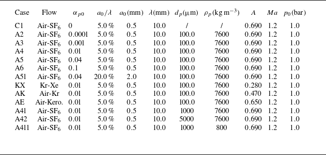
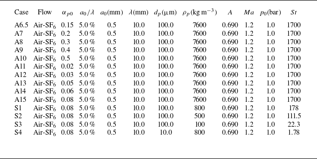
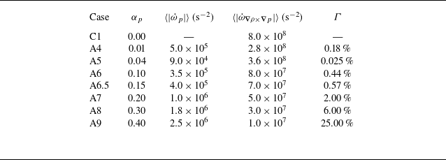
We design a series of numerical simulations to further validate the proposed theoretical model (see table 2) and to compare key physical phenomena (see table 3). Specifically, Cases C1–A6 in table 2 are used to investigate the effect of varying the initial particle volume fraction ( $\alpha _{p0}$ ). The influence of the initial disturbance amplitude ( $a_0$ ) is examined by comparing Cases A5 and A51. Cases A4, KX, AK and AE are designed to validate the model under different Atwood numbers. Finally, the effects of particle diameter ( $d_p$ ) and particle density ( $\rho _p$ ) are explored through Cases A4, A41, A42 and A411. In table 3, additional Cases A6.5–A10 are designed to examine the behaviour under extremely dense particle-laden conditions across a range of initial particle volume fractions. Further Cases A11–A15 are included to extend the discussion of particle volume fraction effects. Moreover, systems with different Stokes numbers are compared through Cases S1–S4.

Table 2.

Verification cases under different initial conditions. The setting of the fluid medium is as follows: for example, if Case C1 flow is Air-SF $_6$ , it means that the left Fluid1 is set to Air and the right Fluid2 is set to SF $_6$ . Here, $\alpha _{p0}$ is the initial particle volume fraction, $a_0$ is the initial amplitude of disturbance, $\rho _p$ is the density of particles, $p_0$ is the preshock background pressure and the preshock temperature is 298 K. The magnitude of $\textit{Re}_p$ is approximately $300- 1500$ and $St\sim 1700$ .

Table 3.

Other cases under different initial conditions. Here, $\alpha _{p0}$ is the initial particle volume fraction, $a_0$ is the initial amplitude of disturbance, $\rho _p$ is the density of particles, $p_0$ is the preshock background pressure and the preshock temperature is 298 K. The magnitude of $\textit{Re}_p$ is approximately $300- 1500$ .

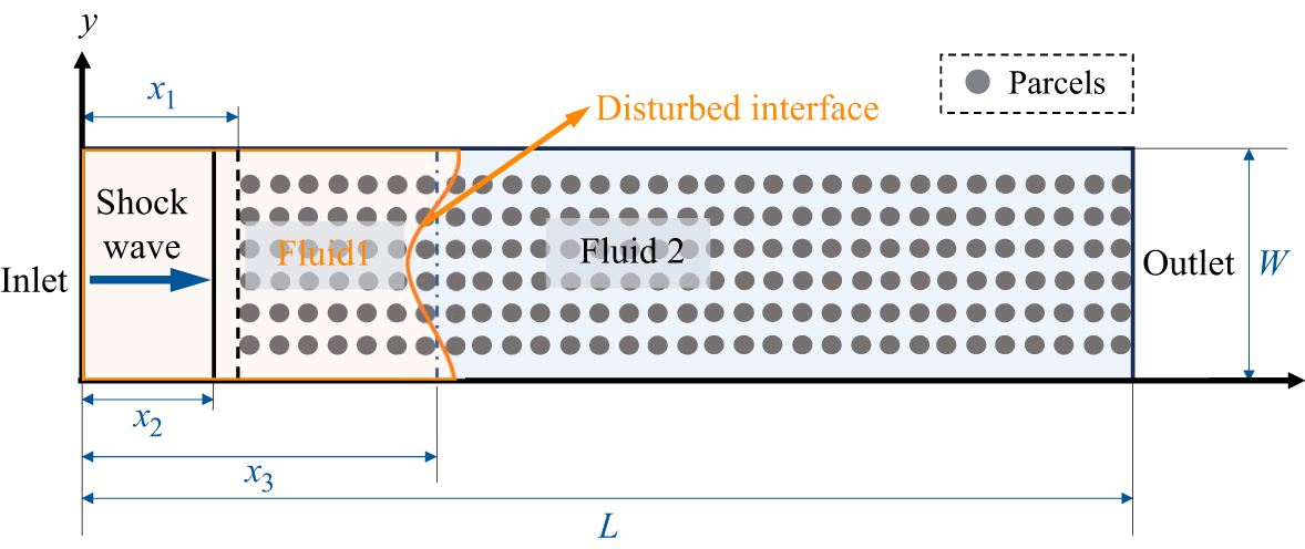
All the simulation cases feature a single-mode perturbed interface, as defined by (3.10). The initial disturbed wavelength and amplitude are $\lambda$ and $a_0$ , respectively. The mean interface position is located at $x_3 = 0.03$ m. Two fluids, denoted Fluid 1 and Fluid 2, form the multiphase interface (see the ‘flow’ column in table 2 for the detailed fluid properties). The computational domain is initialized with a single-mode perturbed interface separating Fluid on the left from Fluid 2 on the right, as illustrated in figure 7. The domain dimensions are $L = 0.12$ m in length and $W = 0.01$ m in width. An incident shock wave with $Ma = 1.2$ is initially located at $x_2 = 0.009$ m. The preshock pressure and temperature in the flow field are 1.0 bar and 297 K, respectively,

(3.10) \begin{equation} x = x_3 - a_0 \cos \left ( \frac {2\pi y}{\lambda } \right ). \end{equation}

Particles are introduced into the flow and are initially distributed uniformly in the region from $x_1 = 0.01$ m to $L = 0.12$ m. All particles are treated as spherical. The initial particle volume fraction within the fluid computational cells is $\alpha _{p0}$ , with particle diameter $d_p$ and density $\rho _p$ . The boundary conditions are specified as follows: the upper and lower boundaries are periodic, while the left and right boundaries are set as the inlet and outlet, respectively. A schematic of the overall computational set-up is shown in figure 7. Detailed parameters for all simulation cases are listed in tables 2 and 3.

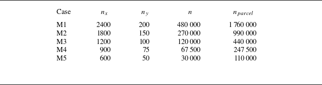
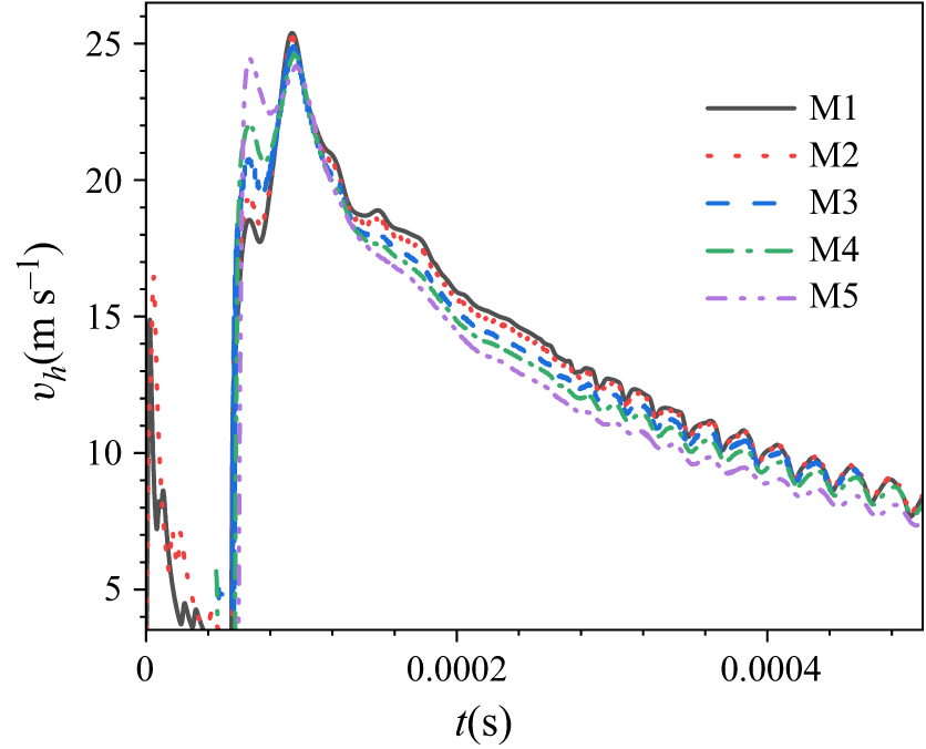
A grid-independence verification study is carried out before the simulations. The specific grid density and particle package set-ups are shown in table 4. Figure 8 shows the time evolution of the mixed zone width growth rate under different grid densities. We find that refinement beyond M2 (1800 $\times$ 150) has a negligible effect on the predicted mixed zone width growth rate. Therefore, M2 (1800 $\times$ 150) is adopted for the subsequent simulations. Further validation of the numerical method for particle-laden RMI can be found in previous studies (Meng et al. Reference Meng, Zeng, Tian, Li, He and Guo2019a ; Si et al. Reference Si, Li, Chen, Meng, Wang and Tian2023, Reference Si, Li, Meng, Wang and Tian2024).

Table 4.

Grid parameters for grid independence verification: where $n_x$ represents the number of grids in the $x$ -direction, $n_y$ represents the number of grids in the $y$ -direction, $n$ represents the total number of grids and $n_{parcel}$ represents the number of particle packages.

Figure 7.

Initial settings and geometrical conditions. The circle represents a schematic diagram of the parcels carrying particles.

Figure 8.

Grid-independence verification results. The fluids in this example are Air on the left and SF $_6$ on the right, and the initial particle volume fraction is $\alpha _{p0}=0.01$ .

3.3. Verification and analysis

We verify the theory through numerical simulations using the CMP-PIC algorithm (Tian et al. Reference Tian, Zeng, Meng, Chen, Guo and Xue2020) (see § 3.1), systematically varying key parameters: particle volume fraction ( $\alpha _{p0}$ ), diameter ( $d_p$ ), density ( $\rho _p$ ), postshock Atwood number ( $A$ ) and initial amplitude ( $a_0$ ) (table 2), with the validity limits of the model assessed.

Figure 9.

The verification and simulation results of this group of examples are both Air-SF $_6$ examples, in which different initial volume fractions ( $\alpha _{p0}$ ) of particles were changed. The specific settings are shown in table 2 for Cases C1, A2, A3, A4, A5, A6. (a) Mixed zone width growth rate; (b) absolute velocities of bubbles and spikes; (c) mixed zone width; (d) comparison between the width of the mixed zone and the theoretical model results; (e) normalized bubbles/spikes velocities versus theoretical predictions; (f) bubbles/spikes relative velocity versus theoretical model.

Figure 10.

The verification and prediction results of the examples in (a), (b), (f) and (g) are all based on changing the Atwood number of the multimedia fluid. Please refer to table 2, Cases A4, AE, AK, KX, for specific settings. In (c) and (h), we present the simulation verification results of different initial disturbance amplitudes ( $a_0$ ) (see table 2, Cases A5, A51, for details). In (d) and (e), we present the simulation verification results of different particle densities and radii (table 2, Cases A4, A41, A42 and A411). (a) Mixed zone width growth rate at different Atwood numbers; (b) absolute velocities of bubbles/spikes at different Atwood numbers; (c) mixing zone growth rate at different initial perturbation amplitudes; (d) mixed zone width growth rate at particle density/radius variations; (e) mixed zone width at particle density/radius variations; (f) normalized bubbles/spikes velocities versus theoretical predictions at different Atwood numbers; (g) bubbles/spikes relative velocity versus theoretical models; (h) normalized bubbles/spikes velocities versus theoretical predictions at different initial perturbation amplitudes.

Figure 11.

(a) Comparison of mixed zone width growth rates for cases with different particle volume fractions ( $\alpha _{p0}\leqslant 0.1$ ). (b) Mixed zone width growth rates for extremely dense particle-laden cases ( $\alpha _{p0}\geqslant 0.1$ ). In these cases, the mixed zone width evolution exhibits a negative perturbation growth rate, indicating that RMI is suppressed in a reverse trend and gradually quenched. (c) Mixed zone width growth rates for different $St$ numbers. These results support the applicability of the large- $St$ model derived in Appendix A.2 when $St\gt 200$ , where the RMI evolution remains similar across cases. They also show that in the small- $St$ regime the behaviour changes fundamentally, with almost no RMI occurring in Case S4.

From figure 9, we first verified the applicability of the theory at different particle volume fractions. As the volume fraction of the particles increases, the growth rate of the mixed zone width over time slows down, and it tends to stabilize earlier, reaching the limit of RMI growth. Figure 11 presents the results of a more extensive numerical simulation of the growth rate of the mixed zone width at different particle volume fractions. The theoretically predicted parameter $\beta$ is the direct indicator of particle effect. The parameter $\beta$ (2.23) increases with larger particle volume fractions ( $\alpha _{p0}$ ) and smaller particle radius, amplifying attenuation through the time-dependent term. Analysing the theoretical model of multiphase RMI dimensionless time $\tau _{\textit{RM}}= ( \alpha kv_0+\beta ) ( 1-e^{\beta t} ) / ( -\beta )$ , multiphase dimensionless time is larger than single-phase dimensionless time and the larger the $\beta$ , the larger the multiphase dimensionless time. The larger the particle volume fraction, the stronger the attenuation in physical time; correspondingly, under the $\tau _{\textit{RM}}$ mapping, the RMI evolution progresses faster in normalized time. As the volume fraction of particles increases, the $\beta$ is larger, and the growth rate of the mixed zone width ( $v_h$ ) decreases, the attenuation becomes faster, and the peak value of the growth rate curve decreases. The decrease in $v_0$ at the beginning of the nonlinear segment is due to the continuous transfer of phase momentum to the particles, resulting in a decrease in velocity in the linear stage of RMI evolution. We also validated the theoretical modelling of mixed zone width, and the results showed good applicability of the theory. Through comparative analysis of numerical simulations, we also found that when the particle initial volume fraction is greater than 0.2, the evolution of the mixed zone width in RMI will reverse and the generation of RMI will be frozen and killed (see figure 11). In such dense particle flow, we focus more on phenomena such as particle jets in engineering applications rather than RMI evolutionary dynamics behaviour (Koneru et al. Reference Koneru, Rollin, Durant, Ouellet and Balachandar2020). In this case, the approximate results of theoretical modelling fail due to significant inertial forces caused by the intense viscous shear between particles and fluids.

As shown in figure 10, we analysed the applicability of the theory for different particle radii and designed three representative cases with distinct radii. We found that as the particle radius increased, the $\beta$ decreased and the growth rate curve decayed more slowly. This is because, while keeping the volume fraction of particles in the flow field constant, the increase in particle size means the decrease in particle number concentration and the drag force experienced by the flow evolution is the sum of the drag forces of each particle, resulting in the decrease in drag force in the flow field and less hindrance to RMI evolution.

In figure 10, we further compared the effects of different particle densities on the attenuation rate. Consistent with theoretical expectations, the attenuation of the growth-rate curves remained nearly indistinguishable as the particle density decreased but the particle radius increased (while maintaining the large- $St$ condition), indicating that the attenuation coefficient is only weakly dependent on particle density. In fact, the damping term $\beta$ in the theoretical model is strictly independent of particle density, which supports the validity of our formulation. We also examined the applicability of the theory at different carrier-fluid density ratios. By considering cases with varying Atwood numbers, we found that larger Atwood numbers led to faster attenuation, in good agreement with the theoretical prediction. Moreover, we tested the theory against different initial perturbation amplitudes and found that these cases also followed the theoretical model. When the initial disturbance amplitude is large, there is a certain degree of deviation in theory.

4.1. Differences in the development of single-phase and multiphase RMI

In this section, we will elaborate on the differences in RMI evolution and development between single-phase and multiphase conditions, based on the differences in disturbance amplitude growth and spikes or bubbles’ finger-like structure evolution.

4.1.2. Differences in morphological finger-like structures

We also studied the influence of particle phase on the interface morphology of RMI evolution in numerical simulations (see figure 12). We found that under the same setting conditions (see figure 12 a), increasing the concentration of particles resulted in differences in the amplitude of interface evolution in the flow field observed at the same time. The higher the particle concentration, the smaller the disturbance amplitude. At the same time, it was also found that in RMI evolution, increasing particle concentration leads to a larger curvature of the spike and a flatter curvature of the bubble. Moreover, under the flow of dense particles, the top of the spike is gradually smoothed out. At the late stage of the nonlinear evolution, we collected the interface evolution morphology of different particle volume fractions $\alpha _{p0}=0$ and $\alpha _{p0}=0.08$ (with the same settings, see figure 12 b). We found that under denser particle loading, the top of the spike becomes flat, and the evolving mushroom-shaped bubble structure develops in a smaller area, with smaller curvature at the bubble. We measured the curvature of the spikes and bubbles in these two examples ( $\alpha _{p0}=0$ and $\alpha _{p0}=0.08$ ), and the results are as follows: the curvature of the spike in the particle volume fraction of $\alpha _{p0}=0$ is approximately $k/6.82$ ( $\xi \sim 1/6.82$ ) and the curvature of the bubble is approximately $k/4.67$ ( $\xi \sim 1/4.67$ ). For particle volume fraction of $\alpha _{p0}=0.08$ , the curvature of the spike is approximately $k/5.76$ ( $\xi \sim 1/5.76$ ) and the curvature of the bubble is approximately $k/6.34$ ( $\xi \sim 1/6.34$ ).

Figure 12.

(a) Contours of the volume-of-fluid field illustrating the evolving RMI interface at $ t = 0.001\,\text{s}$ . The volume-of-fluid function is defined as the volume fraction of one fluid phase volume relative to the domain fluid volume. Subpanel (i) is used to present different interface morphologies at the same time, while the stacked image in (ii) is used to display the differences in curvature of spikes and bubbles. Results are compared for different initial particle volume fractions ( $\alpha _{p0}$ ), under fixed conditions of Stokes number $ St = 1760$ , Mach number $ Ma = 1.2$ and initial amplitude $ a_0 = 0.0005\,\text{m}$ (other settings see tables 2 and 3, Cases C1, A4, A5, A15 and A6). (b) Comparison of the late-stage interface morphology in the nonlinear evolution and the corresponding spike and bubble curvatures for $\alpha _{p0}=0$ and $\alpha _{p0}=0.08$ .

The observed blunting of spikes and flattening of bubbles with increasing particle loading can be attributed to two primary mechanisms: increased momentum dissipation and vorticity suppression. The interphase drag force acts as a distributed momentum sink, extracting energy from the flow. This reduces the kinetic energy available for the sustained growth and sharpening of interface structures. Spikes, which are dynamic, finescale features, are particularly susceptible to this damping effect, leading to their blunted morphology. The development of mushroom-shaped bubble tips and the roll-up of spikes are driven by vortical structures generated primarily through the baroclinic mechanism. As shown in the vorticity dynamics map (figure 17), particles inhibit vorticity generation and amplify its dissipation. Detailed vortex dynamics analysis can be found in § 4.2.2. The consequent weakening of the vortex rings encircling the bubbles limits their ability to roll up and maintain a high curvature, resulting in a flatter, less developed shape. Similarly, the reduced intensity of vorticity strands along the spikes contributes to their smoother appearance.

We also numerically verified the reasonableness of the assumption adopted in our theoretical modelling that the single-phase quasisteady relation serves as a valid approximation. Within the range of particle volume fractions ( $\alpha _{p0}\lt 0.1$ ), the single-phase quasisteady state curvature condition can still be used to construct multiphase models. Actual measurements show that the difference in quasisteady state curvature remains small and does not produce significant deviations in theoretical accuracy. The gradual departure from the single-phase baseline curvature with increasing $\alpha _{p0}$ suggests that future particle-laden RMI models should incorporate a phenomenological correction for the effective interfacial curvature, potentially through a dimensionless parameter that combines particle loading and the Stokes number.

4.1.3. Phenomenon of freeze-out and phase inversion in RMI

Numerical simulations reveal that particle-laden RMI flows exhibit phase inversion, a phenomenon distinct from single-phase RMI. Phase inversion of RMI amplitude emerges when the particle volume fraction exceeds a critical threshold ( $10\,\%$ ). Under these conditions, the mixing zone width transitions from growth to decay (i.e. the growth rate becomes negative see figure 11 b), concurrent with altered anomalous curvature evolution of the interfacial finger structures (see figures 13, 14 and 15).

Comparative analysis of the vorticity fields shows that in phase-inverting, dense particle-laden flows, the dominant interfacial vorticity differs markedly from that in single-phase RMI. Vorticity field visualizations reveal initial negative and positive vortical centres in the upper and lower spike regions, respectively. As the flow evolves, these concentrated vorticity zones weaken until, beyond a critical attenuation level, polarity reversal occurs, triggering amplification of reversed-sign vorticity. In our numerical simulations, a vorticity dynamics analysis (see § 4.2.2 for the methodology) was conducted, isolating the baroclinic vorticity and the particle-induced dominant vorticity – specifically, the particle–fluid curl coupling term. The analysis reveals that this curl-coupling term modifies the interfacial morphology of the RMI under dense particle loading, leading to a reversal of the dominant vorticity polarity, which in turn drives distortion of the interface and a phase reversal and freezing of the RMI, see figure 14.

Figure 13.

Contours of $vof$ and Z-vorticity, illustrating the reversal of the dominant vorticity polarity and the RMI amplitude phase for particle volume fraction $\alpha _{p0}=0.15$ Case A6.5, in contrast to the particle volume fraction $\alpha _{p0}=0$ Case C1. Both show the evolution of the interface morphology and near-interface vorticity field ((a) $\alpha _{p0}=0.15$ ; (b) $\alpha _{p0}=0$ ).

Figure 14.

Contour lines of $vof$ , z-direction vorticity $\omega _z$ , z-direction baroclinic vorticity generation rate $\boldsymbol{\nabla }\!\rho_{\!f}\times \boldsymbol{\nabla }p/{\rho_{\!f}}^2$ , particle–fluid curl coupling vorticity generation rate $\kappa _p\epsilon ( \boldsymbol{\nabla }\times \boldsymbol{u}_p-\boldsymbol{\nabla }\times \boldsymbol{u}_f ) /(\rho_{\!f}V_p)$ for the dense particle-laden case with $\alpha _{p0}=0.15$ .

Figure 15.

Contour lines of $vof$ and z-direction vorticity for dense particle-laden cases with particle volume fractions of (a) $\alpha _{p0}=0.1$ , (b) $\alpha _{p0}=0.2$ , (c) $\alpha _{p0}=0.3$ and (d) $\alpha _{p0}=0.5$ .

4.2. Particle-induced RMI inhibition mechanism

4.2.2. Differences in vorticity dynamics

From the perspective of vorticity, in large $St$ number systems, the vorticity source term caused by particles suppresses the flow field and the generation of baroclinic vorticity, thereby making the disturbance more stable and suppressing the development of RMI.

We derive the vorticity evolution equation from the incompressible momentum equation for the particle-laden flow considered in the nonlinear stage of RMI. The momentum equation is written as

(4.1) \begin{equation} \alpha _f\rho_{\!f}\frac {\mathrm{D}\boldsymbol{u}_f}{\mathrm{D}t}+\boldsymbol{\nabla }\left ( \alpha _fP \right ) =-P\boldsymbol{\nabla }\alpha _p+\frac {\alpha _p\kappa _p}{V_p}\left ( \boldsymbol{u}_p-\boldsymbol{u}_f \right ) +\alpha _f\mu{\nabla} ^2\boldsymbol{u}_f, \end{equation}

where $\alpha _f$ , $\alpha _p$ are the fluid and particle volume fractions and $ \alpha _p+\alpha _f=1$ , $\rho_{\!f}$ is the fluid density, $\boldsymbol{u}_f$ is the fluid velocity, $\boldsymbol{u}_p$ is the particle velocity, $P$ is the pressure, $\kappa _p = 6\pi r_p\mu$ is the Stokes drag coefficient ( $r_p$ , particle radius; $\mu$ , dynamic viscosity) and $V_p = \pi d_p^3/6$ is the volume of a spherical particle ( $d_p$ , diameter).

Figure 16.

The z-direction vorticity magnitude cloud map for different initial particle volume fractions (Cases C1, A4, A5, A15, A6, A9) at $t=0.001$ s. Other settings are listed in tables 2 and 3.

Figure 17.

The z-direction vorticity magnitude cloud map for different $St$ numbers (Cases A15, S1 and S2) at $t=0.0007$ s. Other settings are listed in table 3. The vorticity field shows that the evolutionary behaviour (baroclinic vorticity mechanism) of RMI is similar in large- $St$ number systems. Under small- $St$ numbers, the behaviour is completely inconsistent, with an equivalent Atwood number of approximately zero that diminishes the density gradient, which in turn reduces baroclinic vorticity, preventing RMI development. The vorticity map also shows that as the $St$ number decreases, the vorticity in the flow field becomes larger compared with less than large $St$ numbers.

Figure 18.

The z-direction vorticity magnitude contours of the ‘baroclinic vorticity (I)’ term for different initial particle volume fractions (Cases C1, A4, A5 and A6) at $t=0.001$ s. Other parameters are listed in table 2.

Figure 19.

The z-direction vorticity magnitude contours of the particle-induced vorticity field via the ‘particle–fluid curl coupling (II)’ term, shown for different initial particle volume fractions (Cases C1, A4, A5, A6) at time $t=0.001$ s. Other parameters are listed in table 2.

Figure 20.

The z-direction vorticity magnitude contours of the particle-induced vorticity field via the ‘concentration-gradient coupling (III)’ term, shown for different initial particle volume fractions (Cases C1, A4, A5, A6) at time $t=0.001$ s. Other parameters are listed in table 2.

Figure 21.

The z-direction vorticity magnitude contours of the ‘baroclinic vorticity (I)’ term, shown for different initial particle volume fractions( $\alpha _{p0}=0.15$ , $\alpha _{p0}=0.2$ , $\alpha _{p0}=0.3$ , $\alpha _{p0}=0.4$ ) in dense particle-laden flow (Cases A6.5, A7, A8, A9) at time $t=0.001$ s. Other parameters are listed in table 3.

Figure 22.

The z-direction vorticity magnitude contours of the particle-induced vorticity field via the ‘particle–fluid curl coupling (II)’ term, shown for different initial particle volume fractions ( $\alpha _{p0}=0.15$ , $\alpha _{p0}=0.2$ , $\alpha _{p0}=0.3$ , $\alpha _{p0}=0.4$ ) in dense particle-laden flow (Cases A6.5, A7, A8, A9) at time $t=0.001$ s. Other parameters are listed in table 3.

Figure 23.

The z-direction vorticity magnitude contours of the particle-induced vorticity field via the ‘concentration-gradient coupling (III)’ term, shown for different initial particle volume fractions ( $\alpha _{p0}=0.15$ , $\alpha _{p0}=0.2$ , $\alpha _{p0}=0.3$ , $\alpha _{p0}=0.4$ ) in dense particle-laden flow (Cases A6.5, A7, A8, A9) at time $t=0.001$ s. Other parameters are listed in table 3.

We derive the vorticity evolution equation from the incompressible governing equation under particle loading that controls the nonlinear evolution of the RMI segment of the system. The expression for the momentum equation is (4.1). The next step of transformation is to obtain

(4.2) \begin{equation} \frac {\mathrm{D}\boldsymbol{u}_f}{\mathrm{D}t}=-\frac {\boldsymbol{\nabla }\!P}{\rho_{\!f}}+\frac {\alpha _p\kappa _p}{\alpha _f\rho_{\!f}V_p}\left ( \boldsymbol{u}_p-\boldsymbol{u}_f \right ) +\frac {\mu }{\rho_{\!f}}{\nabla} ^2\boldsymbol{u}_f. \end{equation}

Taking the curl (i.e. applying the nabla operator $\boldsymbol{\nabla }\times$ ) to both sides of the equation yields the following:

(4.3) \begin{equation} \frac {\mathrm{D}\boldsymbol{\omega }_f}{\mathrm{D}t}+\boldsymbol{\omega }_f\boldsymbol{\nabla }\boldsymbol{\cdot }\boldsymbol{u}_f-\boldsymbol{\omega }_f\boldsymbol{\cdot }\boldsymbol{\nabla }\boldsymbol{u}_f=\frac {1}{{\rho_{\!f}}^2}\boldsymbol{\nabla }\!\rho_{\!f}\times \boldsymbol{\nabla }p+\boldsymbol{\nabla }\times \left ( \frac {\alpha _p\kappa _p}{\alpha _f\rho_{\!f}V_p}\left ( \boldsymbol{u}_p-\boldsymbol{u}_f \right ) \right ) +\nu {\nabla} ^2\boldsymbol{\omega }_f. \end{equation}

We define $\epsilon =\alpha _p/\alpha _f$ as the dimensionless concentration ratio. We then obtain

(4.4) \begin{align} \begin{split} \frac {\mathrm{D}\boldsymbol{\omega }_f}{\mathrm{D}t} &+ \boldsymbol{\omega }_f\boldsymbol{\nabla }\boldsymbol{\cdot }\boldsymbol{u}_f - \boldsymbol{\omega }_f\boldsymbol{\cdot }\boldsymbol{\nabla }\boldsymbol{u}_f \\ = \frac {1}{{\rho_{\!f}}^2}\boldsymbol{\nabla }\!\rho_{\!f}\times \boldsymbol{\nabla }p &+ \frac {\kappa _p}{\rho_{\!f}V_p}\epsilon \left ( \boldsymbol{\nabla }\times \boldsymbol{u}_p-\boldsymbol{\nabla }\times \boldsymbol{u}_f \right ) \\ &+ \frac {\kappa _p}{\rho_{\!f}V_p}\boldsymbol{\nabla }\epsilon \times \left ( \boldsymbol{u}_p-\boldsymbol{u}_f \right ) + \nu {\nabla} ^2\boldsymbol{\omega }_f. \end{split} \end{align}

To facilitate the subsequent order-of-magnitude analysis, the governing equation is non-dimensionalized by introducing the following dimensionless quantities (see (4.5)):

(4.5) \begin{align} \begin{aligned} \tilde {x}=\frac {x}{L},\quad \tilde {\boldsymbol{u}}_f=\frac {\boldsymbol{u}_f}{U},\quad \tilde {t}=t\frac {U}{L},\quad \tilde {\boldsymbol{u}}_p=\frac {\boldsymbol{u}_p}{U},\\[3pt]\tilde {P}=\frac {P-P_0}{\rho ^*U^2},\quad \tilde {\rho }_f=\frac {\rho_{\!f}}{\rho ^*},\quad \tilde {\boldsymbol{\nabla }}=L\boldsymbol{\nabla },\quad \tilde {{\nabla} }^2=L^2{\nabla} ^2, \end{aligned} \end{align}

(4.6) \begin{align} Re_L=\frac {UL}{\nu },D_m=\frac {\rho _p}{\rho_{\!f}},St_L=\frac {\rho _pV_pU}{\kappa _pL}, \epsilon =\frac {\alpha _p}{\alpha _f}. \end{align}

Therefore, we obtained the dimensionless result

(4.7) \begin{align} \begin{aligned} &\frac {\mathrm{D}\tilde {\boldsymbol{\omega }}_f}{\mathrm{D}\tilde {t}} +\tilde {\boldsymbol{\omega }}_f\tilde {\boldsymbol{\nabla }}\!\boldsymbol{\cdot }\tilde {\boldsymbol{u}}_f -\tilde {\boldsymbol{\omega }}_f\!\boldsymbol{\cdot }\!\tilde {\boldsymbol{\nabla }}\tilde {\boldsymbol{u}}_f \\ &\;=\underbrace {\frac {1}{\tilde {\rho }_{f}^{2}} \tilde {\boldsymbol{\nabla }}\tilde {\rho }_f\!\times \!\tilde {\boldsymbol{\nabla }}\tilde {p}} _{(\mathrm{I})\ \text{Baroclinic vorticity term}} +\underbrace {\frac {D_m}{St_L}\epsilon \bigl (\tilde {\boldsymbol{\nabla }}\!\times \!\tilde {\boldsymbol{u}}_p -\tilde {\boldsymbol{\nabla }}\!\times \!\tilde {\boldsymbol{u}}_f\bigr )} _{(\mathrm{II})\ \text{Particle-fluid curl coupling}} \\ &\quad +\underbrace {\frac {D_m}{St_L} \tilde {\boldsymbol{\nabla }}\epsilon \!\times \! \bigl (\tilde {\boldsymbol{u}}_p-\tilde {\boldsymbol{u}}_f\bigr )} _{(\mathrm{III})\ \text{Concentration-gradient coupling}} +\underbrace {\frac {1}{Re_L}\tilde {{\nabla} }^2\tilde {\boldsymbol{\omega }}_f} _{(\mathrm{IV})\ \text{Viscous term}}. \end{aligned} \end{align}

The vorticity transport equation reveals several source terms governing the evolution of RMI in particle-laden flows. The first term (I) on the right-hand side of the equation represents the classical baroclinic vorticity term that drives the growth of RMI. The second and third terms (II and III) on the right-hand side of the equation represent particle-induced vorticity source terms, which determine two potential mechanisms for vorticity generation or loss. The second term (II) describes the effect of the vorticity difference between the particle and fluid phases. The third term (III) signifies vorticity generation arising from the misalignment between the particle concentration gradient and the slip velocity. The fourth term (IV) on the right-hand side of the equation represents the viscous contribution to the vorticity evolution.

Subsequently, to assess the relative importance of these mechanisms, we conduct magnitude analysis on each quantity in the dimensionless equation to determine the influence of each term with reference to figures 18–20, where the range of parameter sizes is as follows: $\textit{Re}_L\sim 10^5, St_L\sim 10^2,\epsilon \in [ 0,10^{-1} ], D_m\sim 10^3$ . After conducting a magnitude analysis, we can find that its viscosity term can be neglected. The dimensionless analysis reveals distinct regimes governing vorticity generation in particle-laden RMI. In the deposition vorticity region, the baroclinic term (I) dominates at $O(1)$ , driving classical RMI growth. Particle effects (II, III) remain secondary ( $\lt 10\,\%$ contribution) for limited particle-laden condition ( $\epsilon \in [ 0,10^{-2} ]$ ). In dense particle-laden conditions ( $\epsilon \gt 10^{-1}$ ), the particle terms (II, III) have similar magnitude effects as the baroclinic term (I). In the non-deposition vorticity region, particle terms (II, III) dominate the vorticity evolution and obstruct the generation of vorticity in the flow field.

These predictions are confirmed and elaborated by numerical simulations (figures 18–20). Numerical simulations show that near the vortex core, the second term (II) is almost maximum in the particle-induced term (II, III) due to the high inertia of particles. The vorticity induced by particles (the second term (II)) always opposes the fluid vorticity and is predominantly concentrated in regions of high vorticity in the flow field, specifically the baroclinic vorticity deposition regions. When the fluid vorticity in this region is negative, which is primarily due to the negative baroclinic vorticity term (I), the particle-induced source terms (II) become positive and act to reduce the fluid vorticity magnitude. This mechanism underpins a key finding of the study: the particle-induced vorticity sources suppress the growth of fluid instability, making the development of RMI less pronounced in particle-laden flows. This inhibitory behaviour represents a fundamental distinction between multiphase, particle-loaded RMI and its single-phase counterpart. This conclusion is supported by the vorticity magnitude distribution shown in figure 16, which illustrates that particle effects inhibit the generation of overall vorticity, baroclinic vortex formation and the subsequent evolution of RMI.