1. INTRODUCTION
Some recent attention has been given to the fact that structural equation estimators may have bimodal finite-sample distributions. Phillips and Hajivassiliou (1987) explicitly mentioned the phenomenon, Nelson and Startz (1990) brought the property into prominence, and Maddala and Jeong (1992) provided some further analysis. There has since been a good deal of interest, recent contributions being Woglom (2001), Hillier (2006), Forchini (2006), and Kiviet and Niemczyk (2005). Forchini (2006) studies conditions for the finite-sample distribution of the instrumental variable (IV) estimator to be bimodal, using the factorization of the standard expression of the density (Phillips, 1980) into a leading term and complementary term to find the parameter configurations where bimodality occurs.
A demonstration that the distributions of simultaneous equations estimators were not always unimodal appeared many years ago as a solved (and largely forgotten) exercise in Phillips and Wickens (1978, Sol. 6.19, pp. 351–355), which analyzed the finite-sample distribution of the limited information maximum likelihood/instrumental variable (LIML/IV) estimator in a simple Keynesian structural model. In fact, in this example the finite-sample distribution is always bimodal. The property holds for all parameter values and all sample sizes, although its magnitude is not always practically important. The present paper briefly revisits the Phillips and Wickens example and adds some further analysis and asymptotics to cover weak and very weak instrument cases, where some of the outcomes differ from the results in the conventional weak instrument literature. The model studied by Phillips and Wickens is, in fact, formally equivalent to the model that was considered much later by Nelson and Startz (1990), so there are some interesting linkages to the subsequent literature on the topic.
The Keynesian model is a case of strong endogeneity, where there is a structural behavioral equation and an identity. The identity is another structural relation, and its role is important in the distribution theory because it provides a magnet for an alternative centering, pulling consistent estimators like IV and LIML away from the relevant parameter in the behavioral relation and thereby naturally inducing a bimodality. In fact, it is the identity that is the source of the bimodality. This situation differs in some important ways from the standard case that has been studied intensively in the recent research. The simplicity of the example also means that the key properties of the distribution can be demonstrated analytically in a straightforward way without the use of special functions. For the conditions under which their analysis proceeds, the Nelson and Startz (1990) model is formally equivalent to a structural equation with a companion structural identity, as indicated earlier, and it is the identity that explains the bimodality noted in their paper. This corroborates the comments by Maddala and Jeong (1992) on the role played by strong endogeneity in the occurrence of bimodality.
The fact that identities are common in structural systems makes results for this simple model of more than passing theoretical interest. These results reveal elements in the earlier work on finite-sample theory that have implications on weak instrumentation and weak IV limit theory.
2. STRUCTURAL ESTIMATION WITH AN IDENTITY
The model considered here is based on the simplest Keynesian model with a single structural equation involving two measured endogeneous variables yt, xt, a stochastic disturbance ut, and a parameterized structural identity involv-ing an observed IV zt that is assumed to be exogenous. The system is


where the (spending propensity) parameter β is assumed to satisfy β ≠ 1, so that an equilibrium solution exists. Of course, this condition is needed for the existence of a reduced form and a proper data generating mechanism for the sample data {yt,xt : t = 1,…, n}. The parameter γ controls the relevance of the instrument zt in the system and is convenient to use as a scale coefficient in this equation, but it could readily be absorbed into zt and its effects measured in terms of the signal from the instrument. When γ → 0, the instrument zt becomes irrelevant to the determination of yt and xt, and we end up with the identity xt = yt in place of (2). On the other hand, when γ → ∞, the system is dominated by the signal from zt. In view of the identity (2) and the exogeneity of zt, the degree of endogeneity as measured by the correlation coefficient of xt and ut is unity, so that there is strong endogeneity in the system.
Sometimes it is convenient to extend the model by an array formulation and index one or the other of the parameters γ and β by the sample size n. Use of an indexed sequence γn for γ opens up the study of weak instrument cases, where γn may be passed to zero at certain rates, and use of βn for β enables the model to be analyzed for spending propensities in the vicinity of unity, where βn → 1.
For a finite-sample development, the errors {ut : t = 1,…, n} in (1) may be assumed to be iid N(0,σ2), although Gaussianity is unnecessary for the asymptotics. Phillips and Wickens, like Bergstrom (1962), who first considered finite-sample distributions in this system, allow for an intercept in (1), which is inconsequential, and they did not parameterize (2), setting γ = 1.
Define

. The reduced form is


and β is identified by

The IV or LIML estimator of β is

, where

are the reduced form least squares estimates. Analogous to Bergstrom (1962), Phillips and Wickens (1978) gave the exact density of

:

where λn = γ2szz is the noncentrality parameter. Note that λn depends on the sample size through the sample moment szz but also through the parameter γ when γ = γn depends on n. The exact density (6) is the same as that studied in Nelson and Startz (1990), after notational translation. This is because the model studied by Nelson and Startz (1990) is observationally equivalent to a structural equation with a parameterized identity under the conditioning and zero covariance assumptions that are made in that paper.1
1. Maddala and Jeong (1992) observed that the Nelson and Startz (1990) model is formally equivalent under their stated conditions to the model

for certain parameters θ and φ and where the analysis is conditioned on the supplementary variable vt. The second equation may be rewritten as the parametrized identity

so that the Nelson and Startz (1990) model is equivalent to (1) and (2) after rescaling xt and β and conditioning on vt.
As shown in Phillips and Wickens (1978), the density pdf(b) is continuous and has a zero at b = 1, the same result later being given in Lemma 2 of Nelson and Startz (1990). Rather obviously, the tails are O(b−2), or Cauchy-like (as pointed out in Sargan, 1970/1988, and Phillips, 1983, 1984, 1985, 1986, for structural full information maximum likelihood [FIML] and LIML estimators), and the distribution therefore has modes on either side of the zero at b = 1. Simple calculations reveal that there are two modes located at

where the last two expressions are asymptotic expansions of the modal locations as λn → 0 and λn → ∞, respectively. For small λn, the modes are placed nearly symmetrically on either side of unity at

, and at these points the density is of O(λn−1) as λn → 0. For large λn, one mode is located near β around the value β + 2σ2(1 − β)/λn, and the second mode is located around 2 − β + (λn /2σ2)(1 − β). At this second mode, the density is O(λn−2) as λn → ∞, and so it is negligible in magnitude for large λn.
These properties hold for β ≠ 1 and for all sample sizes n, or all values of the noncentrality parameter λn provided γ ≠ 0. The bimodality disappears asymptotically when λn → ∞ (as happens when γ is fixed and nonzero and n → ∞), because then the distribution of

is asymptotically Gaussian. In this event we have the limit theory

which we can write in standardized form as

which covers the case where β = βn → 1. In the latter case, it is apparent that the presence of a spending propensity in the vicinity of unity raises the convergence rate above

, which is explained by the fact that both the structural equation and the identity work to attract the estimator to unity. Nelson and Startz (1990) argue that the usual Gaussian limit theory is often a very poor approximation to the finite-sample distribution and that it is particularly bad when the instrument is weak. This follows earlier arguments made in Phillips (1989) for the case of irrelevant instruments. However, as we see later, there is an alternative limiting inverse normal theory in this case that provides a very satisfactory approximation to the finite-sample distribution, including its bimodality.
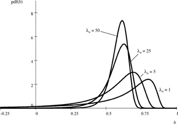
Some typical shapes of the finite-sample density (6) are shown in Figures 1 and 2. For λn = 50, the distribution is close to symmetric, is centered on β, and is well approximated by the Gaussian limit. For λn = 5,1 the distributions are decidedly non-Gaussian in form and show substantial bias and asymmetry, with the mode shifting away from β toward unity as λn decreases. In Figure 1 the mode on the right side of unity is so small that it cannot be seen on this scale, so the right tail of the distribution is omitted from view.

Finite-sample distributions of for β = 0.6 and λn = 1, 5, 25, 50.

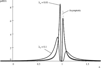
Finite-sample distributions of for β = 0.6 and λn = 0.1, 0.01, and the (very weak) instrument asymptotic distribution (circles).
Figure 2 shows the densities when λn = 0.1, 0.01. Both have marked bimodality. As γ and λn decrease, the pull of the structural identity becomes stronger, and the primary mode shifts closer to unity. As γ and λn decrease further, the secondary mode on the right side of unity becomes more accentuated, and the primary mode shifts even closer to unity. The following intuition explains the bimodality and the location of the modes. Because the IV density is held to zero at b = 1, the secondary mode occurs to the right of unity, much in the same way as a balloon (representing density) is squeezed and a new bubble (mode) arises outside the point of compression to accommodate the density that has been squeezed out elsewhere. Here, the identity serves to provide the point of compression (delivered by the coefficient of the structural identity), and the weak instrumentation provides the energy of compression. Interestingly, the distribution becomes more symmetric again as γ and λn decrease (just as it is for large λn), but now about the value b = 1. Also, although the modes are more peaked and move closer to unity from the right and left sides, the density still descends to zero at unity for all n.
As is clear from the functional form (6), the density pdf(b) does not tend to a proper probability density as λn → 0. In fact, pdf(b) → 0 for all values of b as λn → 0, but not uniformly. So the probability mass escapes at infinity in this case as we take the limit of the density. Nonetheless, we still get convergence of

in this case, but to unity, not to β. In fact,

as λn → 0. Correspondingly, the modes in the density become more peaked and move closer together.
In the limit where γ = 0, we have πy = πx = 0, and the reduced form coefficients contain no information
22. The reduced form error variance σv2 = σ2/(1 − β)2 also contains no recoverable information about β, as σ2 is unknown.

, a.s. for all n. The IV estimator also takes the same value as OLS in this case. This result is different from the distribution in the irrelevant instrument case considered in Phillips (1989), where the IV estimator differs from OLS, is random for all n, and converges to a random variable as n → ∞, unlike OLS, which has a finite nonrandom probability limit.
The result also differs from the limiting case studied in Forchini (2006). Forchini's model is a standard two variable simultaneous system3
3. The model is

where (ut,vt) have covariance matrix

and the concentration parameter is λn = γ′Z′Zγ/σv2.

where 1F1 denotes the confluent hypergeometric function. Forchini shows this limit distribution to be bimodal when θ > 1.
When standardizing transformations are employed so that n−1Z′Z = Ik, the parameter θ has the form

and may therefore be interpreted as the total concentration coefficient because it represents the total amount of “energy” in the reduced form coefficients (γ and β*γ). Note that λn → 0 requires γ′γ → 0 and therefore weak instrumentation. The limiting density (7) includes the totally unidentified case where there is no energy (θ = 0) as in Phillips (1989) and cases where there is some energy (θ > 0) in the coefficients.
As θ increases, we might expect the density to be somewhat more revealing about β*, even when there is weak instrumentation (γ′γ is small), and this is precisely what happens. As θ becomes large, we can use the following simple approximation:

based on the asymptotic expansion of the confluent hypergeometric function 1F1 for large θ (e.g., Lebedev, 1972, p. 271). By a straightforward calculation, the modes of (8) are located at

This approximation is sufficiently accurate, in fact, to capture correctly the criterion for bimodality, namely, θ > 1, given in Forchini (2006).
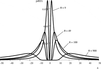
Figure 3 shows the density (8) for various values of θ. Interestingly, as θ increases, the modes in the density (8) move further away from the origin (the point of attraction provided by the least squares estimate and the mode of the IV estimator in the zero energy case), and they diverge with θ. Thus, the modes are drawn toward the two possible limiting values of the standardized structural coefficient, namely, β* = ±∞, which serve as dual attractors based on the point at infinity β*2 = ∞, for which we have ρ2 = 1. Correspondingly, the density becomes less peaked and the modes are less well defined as θ increases. Indeed, mass escapes from the density and pdf(b) → 0 for all b as θ → ∞. The situation here is precisely the opposite of what happens in the case of the density (6), where the modes become more accentuated and move toward the value b = 1, a single attractor provided by the coefficient in the structural identity. In that case, weak instrumentation (γ → 0) is the force behind the movement in the modes and the concentration of the distribution. In the case of the density (8), however, the modes move apart and are drawn to points at infinity corresponding to β* = ±∞, mass escapes to infinity, and the IV estimator of β* diverges. In this event, the force behind the movement in the modes and the divergence of the IV estimator is the energy (θ → ∞) in the reduced form coefficients. Thus, even in the presence of weak instrumentation where γ′γ → 0, the degree of endogeneity increases sufficiently fast (i.e., ρ2 → 1) that the total energy in the reduced form coefficients diverges (θ → ∞), thereby revealing information about β*.

Finite-sample densities (8) of IV estimator for θ = 9, 49, 100, 900.
3. SOME LIMIT THEORY FOR WEAK INSTRUMENTS
Next consider the case where γn depends on n and γn → 0 as n → ∞. The simplest situation of this kind occurs when a local

to zero sequence

is used, an approach that has become conventional in the study of weak instrumentation. Some recent reviews of this literature are given in Andrews and Stock (2005), Hahn and Hausman (2003), and Stock, Wright, and Yogo (2002). Cases of many weak instruments are studied in Chao and Swanson (2005) and Han and Phillips (2006).
The particular

local to zero sequence has no special significance, and limit results may be obtained for other cases. However, we may usefully start with this case, because of its popularity in the literature, and compare results with what happens when γn → 0 at a faster rate. Accordingly, set

, require d ≠ 0, and suppose that the sample second moment of the instrument converges to a positive constant, so that n−1szz → mzz > 0. In this event, the noncentrality parameter tends to a positive constant

and it is apparent that the density (6) has the following limit as n → ∞:

The limit theory in this weak instrument case, analogous to Staiger and Stock (1997), simply reproduces the finite-sample distribution under Gaussianity, a phenomenon that reflects the fact that as n becomes large, the data (and the instrument in particular) become less informative about the true value of the parameter of interest, β. As originally shown in Phillips (1989), it is a straightforward matter to convert the limit result (10) into an invariance principle. All that is required is an appeal to a central limit theorem for the reduced form coefficients on which

depends. In the present case, we have the singular normal limit

and the limit distribution (10) follows in a straightforward manner that is analogous to the finite-sample development. Observe that the limit distribution (10), like the finite-sample distribution, has asymmetric bimodality and Cauchy-like tails.
In place of the conventional weak instrument condition (9), we may consider the very weak instrument case where γn = o(n−1/2) and

In this case, observe that

, so that the systematic part of the reduced form is sufficiently small that the limit theory (11) can be replaced by

where η = (σ/(|1 − β|mzz1/2))ξ and ξ is standard normal. We deduce that

so that

is inconsistent and converges to unity in this case. Some further elementary manipulations
44.

.

the inverse of a central Gaussian variate, and the rate of convergence is given by

. In this very weak instrument case, the systematic part of the reduced form is so small that we do not accumulate information fast enough from the observations (the rate here is still the conventional

rate in view of the behavior of szz) to learn enough about πx and πy to distinguish these parameters from zero. In effect, what we learn from large samples of data is that

are distributed about the origin. Relative to the rate at which γn → 0, we then deduce from the relationship between

in (14) that the estimate

is centered on unity and behaves, after scaling, like the inverse normal variate

.
The asymptotic distribution in the very weak instrument case is shown in Figure 2. As is apparent, the asymptotic distribution provides a good approximation to the finite-sample distribution. Unlike the limit distributions given in (10) and in other weak instrument cases considered in the recent literature, this asymptotic distribution is symmetrically bimodal. It also has zero density at the probability limit of

and continues, of course, to have Cauchy-like tails.
At the point in the parameter space where γ = 0, the data generating mechanism becomes simply yt = xt = ut /(1 − β). This mechanism incorporates the identity (2) and the reduced form equations (3) and (4) with γ = 0. It applies whatever the value of β, and the structural equation (1) is essentially irrelevant to the data generating mechanism. Similarly, when γn → 0 fast enough, the same effects occur. The asymptotic distribution of

is centered about unity (the coefficient in the structural identity yt = xt), the distribution converges at the rate

, which reflects the manner in which the concentration in the data about the structural identity occurs, and the limit distribution provides no information about β when σ2 is unknown.
On the other hand, as remarked earlier, the value of β does affect the reduced form error variance and thereby affects the limit distribution of

about unity. Because this error variance σv2 = σ2/(1 − β)2 → ∞ as β → 1, it follows that 1/η →p 0, as β → 1. We therefore may write (15) in the standardized form

where ξ is standard normal. This result covers the case of a localizing sequence βn for which βn → 1 and then

where the rate of convergence is correspondingly accelerated.
These limit results may be compared with those for the least squares estimator β*, for which standard calculations lead to the following limit theory for the

local to zero sequence

:

and for the very weak instrument case where γn = o(n−1/2):

In both cases β* →p 1 and the limit distribution is normal. There is a noncentrality in the limit distribution for the

local to zero sequence, and the convergence rate is O(n) in this case. In the very weak instrument case, the limit distribution is central normal and the convergence rate is O(nδn), which is faster than O(n). Again, these results extend to the case of a localizing sequence βn for which βn → 1, and then (18), for example, becomes

It follows from these results that, although the IV and OLS estimators have the same limit in probability in the very weak instrument case, their limit distributions and rates of convergence are quite different, so the estimators are not asymptotically equivalent, in contrast to the case where the degree of apparent overidentification is large enough to make the estimators equivalent. In the present case, both IV and OLS estimators are attracted to the same limit point but in a very different manner and at different rates.
In weak identification situations, it is sometimes argued that the IV estimator is drawn toward the least squares estimator.
55. For example, one of the referees refers to “the result that under weak instruments and strong endogeneity the 2SLS estimator is biased towards the least squares value, as discussed by Staiger and Stock (1997).”

local to zero sequences like

, OLS converges at an O(n) rate to the attractor, whereas IV converges to a random variable with the bimodal distribution (10), so it puts probability mass away from and on both sides of the attractor. On the other hand, when the instruments are very weak, we have

, so that the IV estimator has a symmetric bimodal limiting distribution about the least squares value and IV is “drawn to OLS” but in an ambivalent way. Clearly, this is very different from the two estimators being the same in the limit or IV simply being biased toward the least squares value.
4. FURTHER DISCUSSION
In both strong and very weak instrument cases with a structural identity the IV/LIML estimator converges in probability to a constant. In one case, the constant is the true value of the structural parameter β. In the other, it is the coefficient in the structural identity. In conventional weak instrument and irrelevant instrument cases, the estimator converges weakly to a random quantity whose distribution reflects the uncertainty associated with a finite sample of data, as in Phillips (1989). So the presence of a structural identity can lead to substantial changes in weak instrument limit theory.
The finite-sample distribution (and the implied limit distribution under conventional weak instrumentation) is bimodal for all values of the parameters. The source of the bimodality is the presence of an alternative point of attraction provided by the coefficient in the structural identity in the system. The attraction process applies also to OLS but is unidirectional and stronger in the case of OLS and bidirectional and weaker for IV.
The bimodality is of a magnitude to be practically important in cases where the concentration parameter λn is small. As λn becomes very small, the distribution becomes strongly bimodal about the coefficient in the identity, and if λn → 0 the estimator converges in probability to that coefficient at an O(λn−1/2) rate and has a limit distribution that is proportional to the inverse of a standard normal variate and is symmetrically bimodal. By contrast, the OLS estimator converges at an O(nλn−1/2) rate and has a limiting normal distribution.
These results show that, even for the exceedingly simple structural system considered here, weak instrument limit theory has a richer range of possible outcomes than are contained in the present literature.