


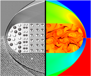

1. Introduction
Shock waves are important phenomenon in supersonic flow and, therefore, shock-induced chemical reactions are of great interest, such as detonation and air dissociation. Detonation waves are supersonic combustion waves induced by shock waves and sustained by the subsequent chemical reactions (Teng & Jiang Reference Teng and Jiang2012). The early observations of detonation originated from mining disasters caused by the accumulation of coal-mine gas and explosions caused by gas leakage from chemical plants. The destructive ability of detonation is much greater than that of ordinary combustion phenomena, and thus it has attracted great attention. Abel (Reference Abel1874) first measured the detonation velocity of cotton powder. After this, Berthelot & Vieille (Reference Berthelot and Vieille1881) systematically measured the detonation velocities produced by mixing various gaseous fuels with different oxidants. This systematic and comprehensive study confirmed the existence of the detonation wave. Since then, detonation has gradually developed into a discipline of experimental, theoretical and numerical investigations with its research category, governing equations and basic laws.
Due to the complexity of the detonation phenomenon, experimental testing has long been the main research method, especially in early studies. Many important physical phenomena have been elucidated through experimental observation. Chatelier (Reference Chatelier1885) recorded the evolution process from deflagration to detonation, and they confirmed for the first time that there can be two combustion modes in the same combustible gas: a deflagration wave and a detonation wave. Denisov (Reference Denisov1959) experimentally observed the cell structure of a detonation wave. Theoretical approaches have also accompanied the development of detonation research. Using the Rankine–Hugoniot (RH) relations, Chapman (Reference Chapman1899) and Jouguet (Reference Jouguet1904, Reference Jouguet1905, Reference Jouguet1916) established theories to analyse the conservation equation of crossing detonation waves, and they obtained the unique solution of the stable propagation velocity of a detonation wave, which is called the Chapman–Jouguet (CJ) velocity. CJ theory is a very important achievement, but it ignores the complex structures of detonation waves. To this end, Zel'dovich (Reference Zel'dovich1940), Von Neuman (Reference Von Neuman1942) and Doring (Reference Doring1943) independently put forward a theoretical model to describe the detonation wave structure, which is referred to as the ZND model. The ZND model successfully combines the chemical reaction process and shock dynamics, establishing a complete theoretical detonation model with a clear concept that considers both physical and chemical phenomena. It thus makes a great contribution to the study of detonation. With the development of computer technology, Taki & Fujiwara (Reference Taki and Fujiwara1978) successfully simulated an unsteady detonation wave for the first time and obtained the three-wave structure of the detonation wave. Eto, Tsuboi & Hayashi (Reference Eto, Tsuboi and Hayashi2005) calculated the propagation of an explosion wave in a three-dimensional pipeline and found the law of three-wave points propagating along the diagonal. Dou et al. (Reference Dou, Tsai, Khoo and Qiu2008) studied the propagation patterns of implosion waves in rectangular pipelines by using a fifth-order weighted essentially non-oscillatory scheme and the third-order total variation diminishing Runge–Kutta method.
In any real detonation, there will always be some curvature of the detonation wave, however small (Sharpe Reference Sharpe2007b). Even a small amount of curvature can have a significant effect on the detonation wave structure (Klein & Stewart Reference Klein and Stewart1993; Yao & Stewart Reference Yao and Stewart1995). Hornung (Reference Hornung1998) solved the inviscid equations of motion for the reacting flow at the downstream side of a curved shock for the shock-normal derivatives and explained the formation of the cellular structure by solving the post-wave streamline curvature. In terms of projectile-induced detonation, Maeda, Kasahara & Matsuo (Reference Maeda, Kasahara and Matsuo2012) and Maeda et al. (Reference Maeda, Sumiya, Kasahara and Matsuo2013) discussed detonation stability owing to the curvature effect arising from the three-dimensional nature of a stabilized oblique detonation wave around a projectile. Their previous studies showed that the detonation wave near the projectile was attenuated below the CJ velocity by the curvature effect (Menees et al. Reference Menees, Adelman, Cambier and Bowles1992; Kaneshige & Shepherd Reference Kaneshige and Shepherd1997). Regarding detonation behind a conical flow, Yang et al. (Reference Yang, Ng, Teng and Jiang2017) performed further simulations to investigate the interplay between the effect of Taylor–Maccoll flow, front curvature and energy release from the chemical reaction in conical oblique detonations. Their simulations showed that the curvature can overcompensate for the high density and temperature in the shocked gas, which means that the curvature plays a more dominant role in the initiation of conical oblique detonation. In the studies of Verreault, Higgins & Stowe (Reference Verreault, Higgins and Stowe2012) and Verreault (Reference Verreault2011), the presence of the curvature was found to allow oblique detonation waves to be initiated at an angle less than that of planar CJ oblique detonation. There have also been some one-dimensional studies, where Watt & Sharpe (Reference Watt and Sharpe2004) performed a one-dimensional study of the stability of weakly curved, quasi-steady detonation waves using a numerical shooting method. Their results show that even weak curvature has a significant destabilizing effect on detonation waves. Sharpe (Reference Sharpe2007a) determined the detonation speed–curvature relations for a small but non-zero front curvature and proposed that slightly curved detonation structures may be helpful for the understanding of cellular detonation.
It is worth noting that in the research of curved shock waves, Mölder (Reference Mölder2016) proposed a curved shock theory in flows with planar or axial symmetry, which was applied to the relationships between pressure gradients, streamline curvature, vorticity and shock curvature. In a subsequent study, curved shock theory was used to calculate flow behind concave shock waves, and the analysis showed that shock curvature plays an important role in determining the flow properties behind double-curved shock waves (Mölder Reference Mölder2017a). In addition, curved shock theory has been applied to calculate flow near single and double curved shock waves, regular shock reflections, and Mach reflections on curved surfaces (Mölder Reference Mölder2017b). Curved shock theory has also been used to discover and demonstrate the effects of longitudinal and lateral wedge surface curvature on the detachment of shock waves from the leading edge of a double curved wedge tip (Mölder Reference Mölder2017c). These studies show that curved shock theory has an active role in the analysis of the flow, reflection and detachment of shock waves. Based on this theory, Shi et al. (Reference Shi, Han, Deiterding, Zhu and You2020) developed a second-order curved shock theory that is a re-derivation of the first-order derivative to obtain the second-order gradients. Further, a method of curved-shock characteristics based on curved shock theory was also constructed (Shi et al. Reference Shi, Zhu, You and Zhu2021). Compared with the method of characteristics, the gradient information enhances the computational efficiency and accuracy of the method of curved-shock characteristics. Moreover, the curved shock theory can be extended to imperfect gases and unsteady flow (Emanuel Reference Emanuel2018). Recently, curved shock theory has been developed to characterize the flow on the downstream side of a three-dimensional shock surface by Emanuel & Mölder (Reference Emanuel and Mölder2022). This study extended the curved shock theory to three dimensions and enhanced its applicability even more. To summarize, on the one hand, curved shock theory can be employed for analyses such as flow after curved shock waves, shock reflections and detachment. On the other hand, curved shock theory can also be developed for unsteady, imperfect gases and three-dimensional curved shock waves. These opportunities demonstrate the significant research value and potential of the curved shock theory. In the meantime, inspired by the CJ theory and the ZND model, if the variations within the reaction zone are not required, a detonation wave can be considered as a reacting shock wave in which reactants transform into products and are accompanied by energy release.
For shocks with chemical reactions, it can be categorized into exothermic or endothermic depending on the specific chemical reaction. For example, detonation waves are generally induced by a shock to produce an exothermic chemical reaction. Combustible gases (e.g. hydrogen) undergoing shock will rise in temperature and pressure to reach combustion conditions, which will then initiate combustion. For example, hydrogen  ${{\rm {H}}_2}$ reacts with oxygen
 ${{\rm {O}}_2}$ to form water
 ${{\rm {H}}_2}{\rm {O}}$. This process will release a large amount of energy and the chemical energy will be converted into heat energy, as shown in figure 1(b). Another classic endothermic reaction type is the air dissociation, where pure air will also increase in temperature and pressure after the shock, and, after reaching certain conditions (generally speaking, very high temperature), the air will dissociate. For example, the nitrogen molecule
 ${{\rm {N}}_2}$ will dissociate into two nitrogen atoms and the oxygen molecule
 ${{\rm {O}}_2}$ will dissociate into two oxygen atoms, and this process will absorb energy, as shown in figure 1(c). When the combustible gas or pure air does not reach the chemical reaction conditions, a shock wave will be formed, as shown in figure 1(a). However, according to the shape of the wave, more specifically the two curvatures in the planar and transverse directions, the wave can be classified into four types. Taking the detonation wave as an example, the first type is an oblique detonation wave without any curvature, as shown in figure 1(d), the second is a two-dimensional curved detonation wave with planar curvature, as shown in figure 1(e), the third is an axisymmetric detonation wave with transverse curvature, as shown in figure 1(f), and the fourth is a curved detonation wave with curvatures in both directions, as shown in figure 1(b). To the best of the author's knowledge, there is no established theoretical method to systematically examine the effect of curvature in planar or conical reaction shock waves.
Schematic diagrams of curved shock waves with experimental or simulation results for reaction and no-reaction: (a) curved shock wave (Lobb Reference Lobb1964); (b) curved detonation wave (Kasahara et al. Reference Kasahara, Arai, Chiba, Takazawa, Yu and Matsuo2002); (c) curved dissociated air (Wen, Massimi & Shen Reference Wen, Massimi and Shen2017); (d) oblique detonation without curvature (Choi et al. Reference Choi, Kim, Jeung, Ma and Yang2007); (e) two-dimensional detonation with planar curvature (Xiang et al. Reference Xiang, Zhang, Tu, Gao, Huang and Peng2022); (f) axisymmetric detonation with transverse curvature (Han, Wang & Law Reference Han, Wang and Law2019).

Inspired by the gas-dynamic theory of detonation, if the variations within the reaction zone are not required, the Rankine–Hugoniot relations are suitable for linking the upstream and downstream states across the wave (Lee Reference Lee2008). In addition, Cheng, Luo & Dongen (Reference Cheng, Luo and Dongen2010) investigated the effect of heat addition on steady and unsteady flow in relation to condensation-induced waves. Apart from that, an instantaneous heat release CJ detonation model was considered to study the Mach reflection of the detonation wave by Bdzil & Short (Reference Bdzil and Short2016). Inspired by these studies, a simplified reaction shock based on conservation laws is studied. The main difference between a reaction shock wave and no reaction shock wave in Rankine–Hugoniot relations is the energy release. To clearly elucidate the energy effect, we simplified the process of chemical reactions, as shown in figure 2. Here,  $\tau _1$ is located in front of the wave,
 $\tau _2$ is located in the wave and
 $\tau _3$ is just behind
 $\tau _2$. The energy released from
 $\tau _1$ to
 $\tau _2$ is denoted as
 $Q_{{d}}$, and the energy released from
 $\tau _2$ to
 $\tau _3$ is recorded as
 $Q_{{c}}$. In other words,
 $Q_{{d}}$ is the energy released when crossing the wave, while
 $Q_{{c}}$ represents the energy released after the wave. Here, the wave can be a shock wave, as well as a dissociation or detonation wave. Therefore, it is worth clarifying again that the theoretical research in this paper is primarily for, but not limited to, detonation; it also applies to all shock-induced chemical reactions with an energy effect. As such,
 $Q_{{d}}$ and
 $Q_{{c}}$ can either be positive or negative and can also degenerate to zero. For example, when considering a detonation wave,
 $Q_{{d}}$ is positive, while considering the dissociated air,
 $Q_{{d}}$ is negative. In pathological detonations,
 $Q_{{c}}$ has a negative value; in CJ detonations,
 $Q_{{c}}$ is equal to zero; as for the other shock-induced combustion where the post-wave is a chemical non-equilibrium,
 $Q_{{c}}$ is positive.
Simplified chemical reaction process in the shock-coupled chemical reaction,  $\tau _1$ is the reactants for the incoming flow,
 $\tau _2$ represents the flow in the reaction zone and
 $\tau _3$ indicates the products after the reaction wave.

In recent decades, with the progress of detonation research and application, related numerical simulations and experimental observations have made great achievements. However, there are few breakthroughs in the theoretical study, so the CJ theory and ZND model are still the main representative works even though they were proposed decades ago. This greatly limits the profound understanding of detonation phenomena and hinders further applications. Therefore, an innovative breakthrough on theoretical research is urgently needed. Under such a motivation, considering the connection between shock and detonation waves, this paper supplements the energy effect on the basis of curved shock theory to make it applicable to detonation. By mathematical derivation in § 2, the curved detonation equations with energy effect are established and the relation between the pre- and post-wave gradients is developed. The influence coefficients are derived and subsequently used in the analysis of post-wave gradients in § 3. The verification is confirmed by a comparison with numerical simulation between the pressure gradients and the streamline curvatures in § 4. The results also suggest that the curved detonation equations can be a quick and effective method to forecast the post-wave gradients. Subsequently, the theory is applied in three aspects. First, polar curve analysis with gradients is proposed in § 5 to complement the previous polar analysis. Then the theory is applied to the capture of detonation waves in § 6, and by comparison with RH relations, the detonation wave captured through higher-order equations is more accurate. Finally, the theory can be used for the inverse design of detonation waves. The above analysis and applications show the unique benefits and potential value of the theoretical method proposed in this paper. Conclusions and future prospects are given in § 7.
2. Curved shock theory supplemented by energy effect
2.1. Derivation of curved shock theory supplemented by energy effect
A curved shock theory supplemented by the energy effect is determined in this section. The energy effects are mainly reflected in two aspects, one is the energy released/absorbed when crossing the shock and another part is the energy change following the shock.
2.1.1. Rankine–Hugoniot equations with energy effect
From figure 2, it is clear that the energy release  $Q_d$ will affect the Rankine–Hugoniot equations. As such, to describe the relationship between the airflow parameters before and after the curved detonation wave, a simplified curved detonation wave is shown in figure 3. Here,
 $V_1$ is the incoming velocity vector and
 $V_2$ is the leaving velocity vector. The flow-deflection angle
 $\delta$ is equal to the difference between the two angles of velocity to the
 $x$-axis, that is,
 $\delta =\delta _2-\delta _1$. The length measured along the detonation wave is
 $\sigma$, and this can be decomposed into the sum of two vectors
 $s$ and
 $n$, which are the length measured tangential and normal to the streamline, respectively. The detonation angle
 $\theta$ is defined as the angular difference between
 $\sigma$ and
 $V_1$. The planar curvature
 $S_{{a}}$ is denoted by the radius of curvature
 $R_{{a}}$, which means that
 $S_{{a}}=-1/R_{{a}}=\partial \theta _1/\partial \sigma$. By the same token, the transversal curvature
 $S_{{b}}$ is represented by
 $S_{{b}}=-1/R_{{b}}=-\cos \theta _1/y$, where
 $y$ is the distance from the detonation to the
 $x$-axis. According to the parameters and assumptions given above, the basic Rankine–Hugoniot equations of a curved detonation wave can be derived as
 \begin{equation} \left.\begin{gathered} {\rho _1}{V_{1{{n}}}} = {\rho _2}{V_{2{{n}}}},\\ {p_1} + {\rho _1}{V_{1{{n}}}}^2 = {p_2} + {\rho _2}{V_{2{{n}}}}^2,\\ \frac{\gamma_1 }{{\gamma_1 - 1}}\frac{{{p_1}}}{{{\rho _1}}} + \frac{{V_{1{{n}}}^2}}{2} + {Q_{{d}}} = \frac{\gamma_2 }{{\gamma_2 - 1}}\frac{{{p_2}}}{{{\rho _2}}} + \frac{{V_{2{{n}}}^2}}{2}, \end{gathered}\right\} \end{equation}
where  $\rho$ is the density,
 $p$ is the pressure,
 ${V_{{{n}}}}$ is the normal velocity and
 $\gamma$ is the specific heat ratio. Subscripts 1 and 2 denote pre-wave and post-wave, respectively. Additionally, the chemical reaction can be calculated by a single-step Arrhenius reaction:
 \begin{equation} \bar\omega =k(1-Z)\exp ({-}Ea/RT), \end{equation}
where  $\bar \omega$ is the chemical reaction rate,
 $k$ is the prefactor,
 $Z$ is the chemical reaction process,
 $Ea$ is the activation energy of the chemical reaction, and
 $R$ and
 $T$ are the gas constants and temperature, respectively. The energy release through the chemical reaction can thus be calculated as
 \begin{equation} {{Q}_{{d}}}={{Q}_{0}}({{{Z}}_{1}}-{{{Z}}_{2}}), \end{equation}
where  ${{Q}_{0}}$ is the total energy released when the chemical reaction is completed. In the single-step chemical reaction model,
 $Z_1$ and
 $Z_2$ denote the pre-wave and post-wave chemical reaction processes, respectively. Here,
 $Z_1=1$ for pre-wave, and
 $Z_2$ can obtain different values according to different chemical reaction progresses and it will be 0 when the reaction is completed. Based on (2.1), a formula for the post-wave parameters can be derived, which is given in Appendix A. To validate the formulation given in this paper, a comparative example is presented. In this paper, the post-wave parameters are first calculated by the ZND theory. After that, the energy released during the detonation can also be calculated. In this way, the post-wave parameters can be solved according to the derivation in Appendix A. The calculation results obtained by the two methods are compared in table 1, and it is easy to find that the post-wave parameters calculated by the RH relations with energy release are very close to the results obtained by the ZND model, so the post-wave parameters calculated in this paper are considered to be credible. The advantage of the present RH relations with energy release over the ZND model is that the relatively accurate post-wave parameters can be acquired without considering the complex chemical reaction, but instead by only solving the aerodynamic equations. Moreover, the relationship between each parameter is expressed as a relatively simple explicit form, which greatly simplifies the difficulty of the detonation solution and helps to enhance the understanding of the aerodynamic relationship of the detonation.
Curved detonation wave with airflow parameters in planar flow, velocity and pressure change in airflow through the curved detonation wave. Curvature  $S_a$ is expressed as the radius of curvature
 $R_a$,
 $S_{{a}}=-1/R_{{a}}=\partial \theta _1/\partial \sigma$,
 $\theta _1=\theta +\delta _1$. Here,
 $p_1$ is the pre-wave pressure and
 $p_2$ is the post-wave pressure in detonation.

Comparison of post-wave parameters calculated through ZND solution (Zhang et al. Reference Zhang, Wen, Zhang, Liu and Jiang2022) and RH equations with energy release. The hydrogen–air mixture is 0.42 ${\textrm {{H}}_2}$+0.21
 ${\textrm {{O}}_2}$+0.79
 ${\textrm {{N}}_2}$ (equivalent ratio is 1), and the pre-wave temperature
 $T_1=300$ K,
 $p_1=1$ atm,
 $u_1=2500$ m s
 $^{-1}$. The ZND structure is calculated by the 9-species 19-reaction by the Jachimowski (Reference Jachimowski1988) mechanism.

2.1.2. Euler equations with energy effect
Something else that will be affected by energy release is the post-wave governing equations. Here, the Euler equations with energy release  $Q_c$ will be introduced. In contrast to shock waves, the Euler equations with energy release in the natural or intrinsic streamline coordinates are used as the governing equations for steady planar or axial flow in the following form:
 \begin{equation} \left.\begin{gathered} \frac{\partial }{{\partial s}}\rho V{y^j} + \rho V{y^j}\frac{{\partial \delta }}{{\partial n}} = 0,\\ \rho V\frac{{\partial V}}{{\partial s}} + \frac{{\partial p}}{{\partial s}} = 0,\\ \rho {V^2}\frac{{\partial \delta }}{{\partial s}} + \frac{{\partial p}}{{\partial n}} = 0,\\ \frac{{\partial h}}{{\partial s}} + V\frac{{\partial V}}{{\partial s}} + \frac{{\partial {Q_{{c}}}}}{{\partial s}} = 0,\\ \frac{{\partial h}}{{\partial n}} + V\frac{{\partial V}}{{\partial n}} + \frac{{\partial {Q_{{c}}}}}{{\partial n}} = 0, \end{gathered}\right\} \end{equation}
where  $j$ is 0 or 1 for planar or axial flow. To simplify the subsequent calculation and keep the form neat, curved shock theory defines the following variable gradients:
 \begin{equation} P = \frac{1}{{\rho {V^2}}}\frac{{\partial p}}{{\partial s}},\quad D = \frac{{\partial \sigma }}{{\partial s}},\quad \varGamma = \frac{\omega }{V},\quad \omega = V\frac{{\partial \sigma }}{{\partial s}} - \frac{{\partial V}}{{\partial n}}, \end{equation}
where  $P$ is the normalized pressure gradient,
 $D$ is the streamline curvature,
 $\omega$ is the vorticity and
 $\varGamma$ is the normalized vorticity. To simplify the influence brought about by the energy release, we also define the following three mathematical coefficients:
 \begin{align} H = \frac{{1 - \rho (\gamma - 1){Q_{{c}}}/V}}{{1 - {\rho ^2}(\gamma - 1){Q_{{c}}}V/\gamma p}},\quad N = \frac{{V - (\gamma - 1)\rho {Q_{{c}}}}}{{V - (\gamma - 1)\rho {M^2}{Q_{{c}}}}},\quad J = \frac{{V + \rho {Q_{{c}}}}}{{V - (\gamma - 1)\rho {M^2}{Q_{{c}}}}}. \end{align}
With the help of these mathematical symbols, we can rewrite (2.4) in the following form:
 \begin{equation} \left.\begin{gathered} \frac{{\partial \delta }}{{\partial n}} ={-} (H{M^2} - 1)P - j\frac{{\sin \delta }}{y},\\ \frac{1}{V}\frac{{\partial V}}{{\partial s}} ={-} \frac{1}{{\rho {V^2}}} \frac{{\partial p}}{{\partial s}} ={-} P,\\ \frac{1}{{\rho {V^2}}}\frac{{\partial p}}{{\partial n}} ={-} \frac{{\partial \delta }}{{\partial s}} ={-} D,\\ \frac{1}{\rho }\frac{{\partial \rho }}{{\partial s}} = H{M^2}P,\\ \frac{1}{\rho }\frac{{\partial \rho }}{{\partial n}} ={-} {M^2}[ND + (\gamma - 1)J\varGamma ],\\ \frac{1}{V}\frac{{\partial V}}{{\partial n}} = D - \varGamma. \end{gathered}\right\} \end{equation}
The detailed derivation process for these equations is shown in Appendix B. It should be explained here that when the energy release  $Q_{{c}}$ is 0, the three coefficients
 $H$,
 $N$ and
 $J$ will become 1, so the above equations are consistent with curved shock theory.
2.1.3. Curved shock theory supplemented by energy effect
As described in the previous section, the Rankine–Hugoniot equations can provide the relationship between the zero-order parameters. To further acquire the relationship between first-order gradients for the pre- and post-wave, the partial derivatives of the following equations need to be derived separately:
 \begin{equation} \left.\begin{gathered} {\rho _1}V_1\sin \theta = {\rho _2}V_2\sin ({\theta - \delta}),\\ {p_1} + {\rho _1}V_1^2\sin^2\theta = {p_2} + {\rho _2}V_2^2\sin^2(\theta - \delta ),\\ V_1\cos \theta = V_2\cos (\theta - \delta). \end{gathered}\right\} \end{equation}
For simplicity, only some of the critical derivation steps are shown here, and the complete derivation can be found in Appendix B. The basic derivation process is as follows: first, both sides of the conservation equation (2.8) are simultaneously derived with respect to  $\sigma$; after this, the partial derivatives are decomposed into two derivatives tangential and normal to the streamline,
 ${{\partial \bullet }}/{{\partial s}}$ and
 ${{\partial \bullet }}/{{\partial n}}$:
 \begin{equation} \left.\begin{gathered} {\left(\frac{{\partial \bullet }}{{\partial \sigma }}\right)_1}= {\left(\frac{{\partial \bullet }}{{\partial s}}\right)_1} \cos \theta + {\left(\frac{{\partial \bullet }}{{\partial n}}\right)_1}\sin \theta,\\ {\left(\frac{{\partial \bullet }}{{\partial \sigma }}\right)_2} = {\left(\frac{{\partial \bullet }}{{\partial s}}\right)_2}\cos ({\theta - \delta}) + {\left(\frac{{\partial \bullet }}{{\partial n}}\right)_2}\sin (\theta - \delta), \end{gathered}\right\} \end{equation}
where  $\bullet$ is a notation for generalized parameters, and the subscripts 1 and 2 represent the pre- and post-wave, respectively. Subsequently, after simplifying and organizing, the curved shock theory supplemented by the energy effect can be obtained as follows:
 \begin{equation} \left.\begin{gathered} A_1P_1+B_1D_1+E_1{{\varGamma}_1}=A_2P_2+B_2D_2+E_2{{\varGamma }_2}+C{S_{{a}}}+G{S_{{b}}},\\ A_1^{\prime}P_1+B_1^{\prime}D_1+E_1^{\prime}{{\varGamma}_1}=A_2^{\prime}P_2+B_2^{\prime}D_2+E_2^{\prime}{{\varGamma }_2}+ {C^{\prime}}{S_{{a}}}+{G^{\prime}}{S_{{b}}},\\ A_1^{\prime\prime}P_1+B_1^{\prime\prime}D_1+E_1^{\prime\prime}{{\varGamma}_1}=A_2^{\prime\prime}P_2+B_2^{\prime\prime}D_2+E_2^{\prime\prime}{{\varGamma}_2}+ {C^{\prime\prime}}{S_{{a}}}+{G^{\prime\prime}}{S_{{b}}}. \end{gathered}\right\} \end{equation}
For convenience, these equations are named curved detonation equations (CDEs). It is necessary to point out that the curved detonation equations derived in this paper are complete three equations rather than the two equations form of the curved shock theory, this is because the post-wave vorticity may be an important gradient and not eliminated. It should be noted additionally that the study in this paper only works for equilibrium flows and does not apply to unsteady flows. The coefficients of the pre-wave  $A_1$,
 $B_1$ and
 $E_1$;
 $A_1^{\prime}$,
 $B_1^{\prime}$ and
 $E_1^{\prime}$; and
 $A_1^{\prime\prime}$,
 $B_1^{\prime\prime}$ and
 $E_1^{\prime\prime}$ and the curvatures
 $C$ and
 $G$;
 $C^{\prime}$ and
 $G^{\prime}$; and
 $C^{\prime\prime}$ and
 $G^{\prime\prime}$ are completely consistent with curved-shock theory, so only the post-wave coefficients affected by energy release are listed in this paper:
 \begin{equation} \left.\begin{gathered}
A_2=\sin \theta \cos (\theta -\delta)(2H_2M_2^2-2),\\
A_2^{\prime}=\sin \theta \cos \theta /\sin (\theta
-\delta)+\sin \theta \cos \theta (3H_2M_2^2-4)\sin (\theta
-\delta),\\ A_2^{\prime\prime}=(H_2M_2^2-1)\sin(\theta
-\delta )\tan(\theta -\delta )+\cos (\theta -\delta ),\\
B_2=\sin \theta (1-N_2M_2^2)\sin (\theta -\delta)-\sin
\theta {{\cos }^2}(\theta -\delta)/\sin(\theta -\delta),\\
B_2^{\prime}=[\sin \theta \cos \theta ({-}1-N_2M_2^2{{\sin
}^2}(\theta -\delta )\\ \qquad\qquad\qquad\qquad +\,2{{\sin }^2}(\theta -\delta
)-2{{\cos }^2}(\theta -\delta ))]/\cos (\theta -\delta ),\\
B_2^{\prime\prime}={-}2\sin(\theta -\delta ),\\ E_2={-}\sin
\theta \sin (\theta -\delta)((\gamma -1)J_2M_2^2+1),\\
E_2^{\prime\prime}=\sin(\theta -\delta ) ,\\
E_2^{\prime}={-}\sin \theta \cos \theta {{\sin }^2}(\theta
-\delta ) ((\gamma -1)J_2M_2^2+2)/\cos (\theta -\delta).
\end{gathered}\right\}
\end{equation}
From (2.10) and (2.11), the relationships between the first-order gradients among incoming flow conditions, energy release, curvatures and post-wave parameters are constructed. There are eight variables in the equations:  $P_1$,
 $D_1$,
 $\varGamma _1$,
 $P_2$,
 $D_2$,
 $\varGamma _2$,
 $S_{{a}}$ and
 $S_{{b}}$. As long as five of these are known, the remaining three can be solved by the curved-detonation equations. These equations can be used in the following ways. On the one hand, the post-wave gradients can be solved according to the pre-wave gradients, curvature and energy release, as described in § 4. On the other hand, we can also compute the curvatures according to the pre- and post-wave gradients with the energy release; this could be used in the capture and reverse design of a detonation wave as shown in § 6.
The above derivation process is mainly based on the assumption of instantaneous energy release, which is reasonable for a preliminary study. However, the absence of chemical reaction makes the study incomplete. To cover this weakness, we give the curved detonation equations with chemical reaction (single-step Arrhenius equation) in Appendix C. For convenience, curved detonation equations with chemical reaction are called CDEC to distinguish it from CDE. The relationship between CDEC and CDE can be illustrated from both qualitative and quantitative perspectives. Qualitatively speaking, when the chemical reaction related variables can be neglected, it is reasonable to simplify the effect of the chemical reaction to an energy release treatment, like the CJ theory did. Quantitatively speaking, the smaller errors of the two equations in the solution of post-wave parameters are demonstrated in table 1. Thus, the CDE will be the main one to be applied in the subsequent analysis and applications. Similar analysis and applications can also be performed for the CDEC, but these will not be repeated for the brevity of the article. It should be specifically noted that for some cases, CDEC is necessary such as when the effect of the chemical reaction zone on the curvature of the streamlines cannot be ignored in the two-dimensional problem.
With the help of CDE, the effect of energy release on the zero- and first-order parameters can be analysed separately, as shown in figure 4. For the zero-order parameters, according to classical gas dynamics knowledge, if energy release  $Q_{{d}}$ increases from zero, the
 ${p_2}/{p_1}$ will become smaller. It is known that the post-wave Mach number of a detonation wave is decreased compared with that of a shock wave, which means that the energy release decreases the post-wave Mach number. The detonation angle is also greater than the shock angle. For the first-order parameters, according to (2.5a–d), if
 $M_2^2 > 1$, then the energy release
 $Q_{{c}}$ increases, and all three energy factors
 $H$,
 $N$ and
 $J$ will increase. Conversely, if
 $M_2^2 < 1$, then
 $H$ and
 $N$ will decrease. In short, the energy release has different effects on the zero- and first-order parameters in different situations, and the final effect will not always monotonically increase or decrease the post-wave gradient. This conclusion is also consistent with the patterns of variation in the influence coefficients. In general, the pre-wave pressure gradient has the greatest influence on the post-wave pressure gradient, and the energy release will significantly increase the effect of the pre-wave gradients on the post-wave pressure gradient. This provides a reference for the change in the pressure gradient in the post-wave of detonation.
Analysis of the various energy effects on the curved shock including detonation and dissociation.

3. Analysis with curved detonation equations in influence coefficient format
To better understand the curved detonation equations constructed in the previous section, further analysis will be performed in this section. We first solve the format of the influence coefficients of the post-wave gradients and discuss their variation. The detailed derivation can be found in Appendix D. The effects of energy release are highlighted; it not only affects the zero-order parameters such as  $M_2$, but also changes the first-order gradients through the
 $H$,
 $N$ and
 $J$ coefficients. After this, post-wave gradients under different curvatures are fully discussed to emphasize the impact of curvature when compared with oblique detonation.
3.1. Analysis with the influence coefficients of the pre-wave gradients
As can be seen from Appendix D, the five influence coefficients can be divided into two parts: the former three represent the influence of pre-wave gradients (e.g.  $J_p$,
 $J_d$,
 $J_g$) and the latter two (e.g.
 $J_a$,
 $J_b$) represent the influence of curvature. The influence coefficients of the pre-wave gradients are analysed first; after this, the influence coefficients of the two curvatures are discussed separately because the planar and transversal curvatures have different characteristics. It is worth noting that the specific curves of influence coefficients have a strong relationship with the incoming flow parameters. The detailed parameters given by the example are not universal for all detonation conditions, but the fundamental laws are similar. The incoming flow parameters given in this section are
 \begin{equation} p_1 = 1 \times10^5\,\mathrm{Pa},\quad {\rho _1} = 0.1\,\mathrm{kg}\,\mathrm{m}^{{-}3},\quad M_1 = 10,\quad \gamma_1 = 1.3. \end{equation}
To emphasize the influence of energy release in the detonation wave, various different situations of energy release are considered. When the energy release  $Q_d$ is negative, it means that the shock wave is energy absorbing, which can occur in the dissociation of air. When the energy release
 $Q_d$ is positive, it means that the shock wave is exothermic, which can occur in a detonation wave. Similarly, when the energy release
 $Q_c$ after the wave is negative, this means that there is an energy-absorbing chemical reaction after the wave, which can occur in a pathological detonation. When the energy release
 $Q_c$ after the wave is positive, it means that there is an exothermic chemical reaction after the wave, which may mean that the detonation wave continues to combust after the wave.
The first concern is the effects of the pre-wave pressure gradient, streamline curvature and vorticity on the post-wave pressure gradient, as shown in figure 5. The solid line indicates a shock wave with no energy release and the area charts represent the effects of energy, where the lighter areas show energy absorption ( $Q_d< 0$ or
 $Q_c< 0$) and the darker areas show energy release (
 $Q_d> 0$ or
 $Q_c> 0$). Thus, two aspects should be considered: one is how the influence coefficient varies with different wave angle and the other is how the influence coefficient is affected by various energy release. In figure 5(a), the solid blue curve shows that when the wave angle is between 20
 $^{\circ }$ and approximately 75
 $^{\circ }$, the influence coefficient
 $J_{{p}}$ always remains constant at approximately the same level, and it then decreases to 0. After exceeding approximately 84
 $^{\circ }$, this effect becomes a negative correlation and gradually increases to a peak negative value over
 $-1000$. This curve will reach a maximum at 90
 $^{\circ }$, meaning that a normal detonation wave has the largest influence coefficient when compared with oblique/curved detonation waves. In addition, at values of approximately 84
 $^{\circ }$, the pressure gradient of the incoming flow has no effect on the pressure gradient behind the wave. The solid green curve, which represents the influence coefficient
 $J_{{d}}$, shows that the pre-wave streamline curvature makes a negative contribution to the post-wave pressure gradient for all wave angles. In the range of acute angles, this action law first increases gradually, then decreases to a minimum, and it reaches its maximum value at approximately 85
 $^{\circ }$. Moreover, this contribution is 0 at the 90
 $^{\circ }$ point. This means that for positive detonation, the pre-wave streamline curvature has no effect on the post-wave pressure gradient at this point. The solid red curve, which represents the influence coefficient
 $J_{{g}}$, reveals that the contribution of the pre-wave vorticity to the post-wave pressure gradient is similar to that of the green curve, peaking at approximately 85
 $^{\circ }$. In figure 5(b), the pattern of the effect of energy release (
 $Q_c$) is however different, for example, for the blue curve
 $J_{{p}}$, the peak of the effect is no longer located at 90
 $^{\circ }$, whereas both
 $J_{{d}}$ and
 $J_{{g}}$ take their maximum at 90
 $^{\circ }$. This difference occurs because the energy effects of the two types act in different ways.
Influence coefficients of pre-wave gradients to the post-wave pressure gradient. (a)  $Q_d$ with positive, zero and negative values. (b)
 $Q_c$ with positive, zero and negative values.

Figure 6(a,b) depicts the influence of pre-wave gradients on the post-wave streamline curvature. It can be seen from the solid blue curve that  $K_{{p}}$ keeps positive when wave angles are small, which means that the pre-wave pressure gradient will enhance the post-wave streamline curvature in this range. The curve subsequently becomes negative after crossing a point over 50
 $^{\circ }$. As the wave angle continues to increase, the pre-wave pressure gradient has less effect and reaches a minimum. When it reaches 90
 $^{\circ }$, there is no effect on the post-wave streamline curvature, which means that no matter how much the pressure is changed, the post-wave streamline curvature will not be affected. It can be seen that the solid green curve
 $K_{{d}}$ rises from the acute angle range and reaches a maximum value near 90
 $^{\circ }$. The solid red curve
 $K_{{g}}$ shows that the influence law is similar to that of the green curve, but the values are smaller.
Influence coefficients of pre-wave gradients to the post-wave streamline curvature. (a)  $Q_d$ with positive, zero and negative values. (b)
 $Q_c$ with positive, zero and negative values.

The effect of energy release in  $K_{{p}}$ is larger when the wave angle is smaller, which can be seen in the area chart in figure 6(a,b), and it gradually decreases as it approaches approximately 60
 $^{\circ }$. This means that at smaller wave angles, the energy release causes a significant change in the effect of the pre-wave pressure gradient on the post-wave streamline curvature; conversely, in a normal detonation wave, the effect of the energy release in
 $K_{{p}}$ is very small. In figure 6(a), the pattern of the green areas are different, and the green areas becomes 0 near 86
 $^{\circ }$. This means that at this point, the pre-wave streamline curvature has an equal influence on the post-wave streamline curvature for the shock, dissociation and the detonation; after that, the effect of the detonation and dissociation wave is significantly stronger than that of the shock wave. The changes in the green and red line as well as areas are similar, and this implies that the pre-wave vorticity and streamline curvature make similar contributions to post-wave streamline curvature. Generally speaking, the post-wave streamline curvature is most affected by the pre-wave streamline curvature and the maximum is achieved in a normal detonation wave; this is easy to understand intuitively and it is consistent with the laws of physics.
Figure 7 shows the variation of post-wave vorticity with incoming flow conditions. The blue curve  $F_{{p}}$ first decreases and then increases in the range of negative values, reaching a maximum just over 80
 $^{\circ }$. The coefficient is zero at 90
 $^{\circ }$, which means that the pre-wave pressure gradient does not affect the post-wave vorticity in normal detonation. The variation trends in the green curve
 $F_{{d}}$ and the red curve
 $F_{{g}}$ are similar, but their specific values are different. Both curves reach their maximum absolute value at 90
 $^{\circ }$, and they are not zero-valued at any point, which means that these two coefficients are always present across the whole angular range. The blue areas are in opposite positions in figure 7(a,b), which means that the effects of
 $Q_{{d}}$ and
 $Q_{{c}}$ are different, with
 $Q_{{d}}$ enhancing the effect of
 $F_{{p}}$ and
 $Q_{{c}}$ weakening the effect of
 $F_{{p}}$. A similar analysis applies to the
 $Q_{{d}}$ and
 $Q_{{c}}$ for
 $F_{{d}}$ and
 $F_{{g}}$. Figure 7 also shows that the pre-wave streamline curvature is still the biggest factor affecting the post-wave vorticity, and this is followed by the pre-wave pressure gradient and vorticity.
Influence coefficients of pre-wave gradients to the post-wave vorticity. (a)  $Q_d$ with positive, zero and negative values. (b)
 $Q_c$ with positive, zero and negative values.

In these three figures, the pre-wave streamline curvature and vorticity action laws are always similar. This may be caused by the presence of the same parameter:  $\partial \sigma /\partial s$. In addition, we can see that energy release always has a significant effect, which means that separate research is required to examine detonation waves, dissociations and simple shock waves. The fundamental reason for this difference is that the energy release will change the post-wave zero-order parameters with the influence coefficients of first-order gradients, and it will thus also change the first-order gradients. The energy release at different locations has completely different effects on the post-wave first-order gradients and these effects are also non-monotonic. These curves and their analysis help us to understand more clearly the variation patterns of detonation, and they also highlight the effect of energy release.
3.2. Analysis with influence coefficients of detonation curvature
Now that the pre-wave influence coefficients have been analysed, analysis with the influence coefficients of the detonation curvature should be performed. To exclude the influence of pre-wave gradients, the incoming flow parameters are set to be uniform, which means that the equations with influence coefficients can be simplified to
 \begin{equation} \left.\begin{gathered} P_2 = {J_{{a}}}{S_{{a}}} + {J_{{b}}}{S_{{b}}},\\ D_2 = {K_{{a}}}{S_{{a}}} + {K_{{b}}}{S_{{b}}},\\ {\varGamma _2} = {F_{{a}}}{S_{{a}}} + {F_{{b}}}{S_{{b}}}. \end{gathered}\right\} \end{equation}
The post-wave gradients will be different for planar and axial problems; as such, the system is examined separately from these two perspectives.
3.2.1. Analysis with influence coefficients of planar curvature
For two-dimensional curved detonation waves, there is no transversal curvature, which means that  $S_{{b}}$ is zero. Then, (3.2) can be simplified to
 \begin{equation} \left.\begin{gathered} P_2 = {J_{{a}}}{S_{{a}}},\\ D_2 = {K_{{a}}}{S_{{a}}},\\ {\varGamma _2} = {F_{{a}}}{S_{{a}}}. \end{gathered}\right\} \end{equation}
In such a case, the post-wave first-order gradient parameters are drawn as shown in figure 8. The curvature is set to  $-$1, which means that
 $P_2 = -J_{{a}}$,
 $D_2 = -K_{{a}}$ and
 $\varGamma _2 = -F_{{a}}$.
Post-wave first-order gradients of two-dimensional detonation waves in uniform flow. (a)  $Q_d$ with positive, zero and negative values. (b)
 $Q_c$ with positive, zero and negative values.

In figure 8, the blue curve shows that under a given uniform incoming flow and constant curvature, the post-wave pressure gradient reaches its absolute maximum at 90 $^{\circ }$. This means that the post-wave pressure gradient will be at its maximum when oblique detonation is converted to normal detonation. In addition, at approximately 85
 $^{\circ }$, the post-wave pressure gradient is zero; this is referred to as the Thomas point (Thomas Reference Thomas1947). The effect of energy release is always apparent, especially when the wave angle is small. The green curve represents the post-wave streamline curvature. This first increases and then decreases in the acute angle range, and it reaches a maximum at approximately 83
 $^{\circ }$. In addition, the post-wave streamline curvature is zero at approximately 76
 $^{\circ }$; this is an important parameter to determine the flow situation after the wave, and it is called the Crocco point (Crocco Reference Crocco1937). The red curve represents the change of post-wave vorticity, which first increases and then decreases in the acute angle range, reaching a maximum at approximately 85
 $^{\circ }$; the vorticity is zero at 90
 $^{\circ }$. Another principle can be observed from figure 8: the energy release changes the locations of the Thomas and Crocco points, once again demonstrating that the effect of energy release is not negligible.
To illustrate the correspondence between these curves and the detonation wave more clearly, figure 9 displays the distribution of the streamline curvature after a curved detonation wave. Figure 9(a) shows several streamlines of the air dissociation flow field, where the chemical reaction takes the results of the study of Park (Reference Park1985). Expressing the results of figure 9(a,b), it is not difficult to notice the effect of curvature on the flow. Herein, point 1 corresponds to the negative curvature of the streamline in figure 8, and point 2 corresponds to the Crocco point, where the curvature of the streamline is zero. Point 3 is the positive curvature of the streamline after the Crocco point, and point 4 corresponds to the angle of the detonation wave being 90 $^{\circ }$, that is, a normal detonation wave. Points 5, 6 and 7 are then the positions in the obtuse-angle section corresponding to points 3, 2 and 1, respectively.
Post-wave streamline curvatures of a planar detonation wave in uniform flow. The initial conditions for the numerical simulation are pressure is 1.96 atm, temperature is 206 K, Mach number is 38 Mach and the incoming flow is pure air.

Curvature plays a crucial role in curved shocks and curved detonations. Therefore, it is necessary to investigate the effect of curvature on the post-wave gradients at different magnitudes and directions. The detonation curvatures can be varied in the planar and axial flow fields to observe the corresponding changes in the first-order gradients. With the above research purpose, we plotted the post-wave pressure gradient, streamline curvature and vorticity for five different detonation curvatures of  $-2$,
 $-1$, 0, 1 and 2, as shown in figures 10, 11 and 12, respectively. In figure 10, different colours represent different magnitudes of detonation curvatures and concavity/convexity is distinguished by the solid/dashed lines. We can first conclude that changing the detonation curvature significantly affects the post-wave pressure gradient, and a larger detonation curvature will lead to an increase in the absolute value of the pressure gradient at all angles. This is consistent with our previous prediction. In addition, detonation waves with different curvatures have the same Thomas point, which means that the detonation curvature does not affect the Thomas point.
Post-wave pressure gradients with different planar curvatures  $S_{{a}}$.

Post-wave streamline curvatures with different planar curvatures  $S_{{a}}$.

Post-wave vorticity with different planar curvatures  $S_{{a}}$.

A similar regularity is also reflected in the post-wave streamline curvature, which is plotted in figure 11, in which it can be seen that a larger detonation curvature increases the curvature of the post-wave streamline across the full range of angles. Similarly, the position of the Crocco point remains unaffected by the detonation curvature. Figure 9(c) helps to illustrate the curvatures of the post-wave streamlines for different detonation curvatures more intuitively: figure 9(c) corresponds to the case with positive curvature, and its variation law has been explained in detail using figure 11; figure 9(d) corresponds to the case in which the detonation curvature is negative, and its variation law can also be seen in the obtuse part of figure 11.
Regarding the post-wave vorticity, we can conclude from figure 12 that this is always monotonous in the acute angle range, and increasing curvature also makes the vorticity larger. The same trend is followed in the obtuse angle range, but with the opposite sign. From the above three plots, it is not difficult to observe that the gradients of the concave and convex detonation waves are symmetric about the oblique detonation.
3.2.2. Analysis with influence coefficients of axial curvature
For an axial detonation wave, the curvature  $S_{{a}}$ is zero and the distance
 $y$ is set to 1. The equations can thus be simplified to
 \begin{equation} \left.\begin{gathered} P_2 = {J_{{b}}}{S_{{b}}},\\ D_2 = {K_{{b}}}{S_{{b}}},\\ {\varGamma _2} = {F_{{b}}}{S_{{b}}}. \end{gathered}\right\} \end{equation}
In such a case, the post-wave first-order gradients are drawn as shown in figure 13. For the axial flow in figure 13, the blue curve shows that the post-wave pressure gradient is also affected by the transversal curvature, which first decreases and then increases, reaching a maximum absolute value at approximately 86 $^{\circ }$. The green curve shows the effect of transversal curvature on the post-wave streamline curvature, reaching a negative maximum at approximately 82
 $^{\circ }$. There is quite a significant difference when this is compared with planar flow: the energy release
 $Q_d$ always enhances the post-wave pressure gradient and streamline curvature. The post-wave vorticity is not shown because the transversal curvature will not affect the post-wave vorticity, as also demonstrated by Mölder (Reference Mölder2016).
Post-wave first-order gradients of axial detonation waves in uniform flow. (a)  $Q_d$ with positive, zero and negative values. (b)
 $Q_c$ with positive, zero and negative values.

Similar to the case of the planar detonation wave, we also plotted the curvature of the post-wave streamline in an axial flow with different detonation-wave angles, as shown in figure 14. Here, point 1 corresponds to the curvature of the streamline in the acute part of figure 13, and the direction of streamline curvature does not change in the process from point 1 to point 3; as with the planar case, the curvature in the normal detonation is zero. The changes in the obtuse angle range are similar and are not described in detail here. As with the planar curvature, to study the effect of different transversal curvatures on the post-wave gradients, we plotted five cases with curvatures of  $-2$,
 $-1$, 0, 1 and 2, as shown in figures 15 and 16. In figure 15, in the acute angle range, the post-wave pressure gradients in the axial flow increase monotonically with increasing curvature. The biggest difference with the planar flow is the absence of Thomas points. Since the curvature value is given directly here instead of the distance
 $y$ in the axial direction, this plot is not similar to the curve in figure 13.
Post-wave streamline curvatures of an axial detonation wave in uniform flow.

Post-wave pressure gradients with different transversal curvatures  $S_{{b}}$.

Post-wave streamline curvatures with different transversal curvatures  $S_{{b}}$.

When discussing the post-wave streamline curvature in the axial flow, we note that in figure 16, if the curvature is negative, the post-wave curvature of the streamline first increases and then decreases in the acute range, but it always remains positive; i.e. there is no Crocco point, which is completely different from the planar flow. This effect is similar when the curvature is positive. However, the curvature of the streamline increases across the range as the curvature of the detonation wave increases, which is similar to the planar flow. As discussed above, the transversal curvature does not affect the post-wave vorticity; as such, the post-wave vorticity is always zero for different curvatures, and this is not shown here specifically. From figure 16, we can see that the streamline curvature after an axial wave is monotonically related to the curvature of the detonation wave. When the transversal curvature is positive, the post-wave streamline curvature is negative, as shown in figure 14(b); accordingly, when the transversal curvature is negative, the post-wave streamline curvature is positive, as shown in figure 14(a).
This section has considered the influence coefficients of curvature in curved detonation and the effects of different values of curvature on the post-wave gradients. These curves can be further applied in the analysis of curved detonation waves; for example, the presence of curvature leads to the divergence/convergence of the post-wave flow, which can change the post-wave temperature, density and pressure. This theory also provides a basis for subsequent analysis and application of detonation waves.
4. Verification of curved detonation equations
After the analysis of the curved-detonation equations, the next step is to verify the validity of the theory. It should be noted here that the theory makes several simplifications to the behaviour of a real detonation, and the value of the energy release is difficult to calculate completely correctly. Therefore, there will be differences between the theoretical and simulation results; the focus here is to study the common law reflected by the two results and explore the influence of energy release and curvature on curved detonation.
4.1. Comparison of post-wave pressure gradients between simulation and theory
As noted before, the post-wave first-order gradient parameters can be derived from the curved-detonation equations for uniform incoming flow conditions. At the same time, we can also obtain the first-order gradient parameters by post-processing the results of the simulation. In this way, theory can be verified by comparing the results of two calculations. For this purpose, we have selected a projectile-induced curved-detonation result. The simulation approach provides a classical example, and this was verified in comparison with experiments, as shown in figure 17. Since the methods of numerical simulation are not the focus of this paper, they will not be described too much, and detailed explanations can be found in our previous study (Yan et al. Reference Yan, Han, Xiong, Shi and You2024). Since aerodynamic parameters such as the post-wave pressure need to be used for comparison, the grid-independence of the numerical method needs to be examined and the detailed validation results can be found in Appendix E. Final results indicate that the grid level adopted in this paper can accurately capture data such as pressure and airflow deflection angle of the detonation. According to figure 17, it can be seen that the simulation results are in good agreement with the experimental results. Not only are the shapes of the detonation waves similar, but even the locations of the points where the shock and combustion waves separate are very close to each other. The reason for this separation is that as the intensity of the detonation wave decays, the induced shock wave is not strong enough to induce detonation combustion, so the induced shock wave and the combustion plane gradually separate, which is an inevitable phenomenon. Also this reminds us that only data prior to the separation point will be selected for subsequent verification. The incoming flow conditions were set to
 \begin{equation} {p_1} = 42\,663\,\mathrm{Pa},\quad {\rho _1} = 0.366\,\mathrm{kg}\,{\mathrm{m}^{{-}3}},\quad M_1 = 6.39,\quad {T_1} = 298\,\mathrm{K}. \end{equation}
The simulation results can be calculated consistent with the experimental incoming flow conditions as shown in figure 18(a). To quantify the gradient of the detonation wave, ten streamlines are selected in this paper and the variation of pressure and hydrogen content on any one of them is plotted, as shown in figure 18(b). It should be noted that these ten streamlines are all on the left side of the red dashed line in figure 17. In other words, the streamlines are located before the decoupling of the shock wave and reaction wave, so it can be considered as a detonation wave. Considering that the thickness of the detonation wave is not negligible, to extract the post-wave parameters, a uniform post-wave definition is adopted in this paper. Taking figure 18(b) as an example, the green curve indicates the mass fraction of hydrogen, which is 0.02851 in the incoming flow and becomes 0.00397 at infinity, which means that the total consumption of the gas is 0.0245. The point A after the wave is chosen, on which the mass fraction of hydrogen is 0.00592, and after calculation, it is known that the hydrogen consumed at this point accounts for more than 92 % of the total consumption; therefore, define this point as the post-wave.
Comparison of the simulated and experimental results of a projectile-induced curved detonation: (a) shadowgraph of simulation result; (b) experiment by Lehr (Reference Lehr1972).

Simulation results: (a) temperature contour; (b) pressure and hydrogen mass fraction along the streamline.

Further, to more concretely show the change in pressure at the post-wave, four streamlines were selected, and the pressure and pressure gradient changes on them are plotted as shown in figures 19 and 20, respectively. From the four curves in figure 19, especially streamline 1, we can see that the first point at which the pressure value increases suddenly is the point referred to as the induced shock in the ZND model. After this, there will be a significant drop, which should correspond to the reaction zone in the ZND model. After this region, whether the pressure value rises or falls depends on the post-wave pressure gradient. In streamline 1, after the reaction zone of the detonation wave, the pressure value rises significantly, which means that the pressure gradient after the wave is positive; at the same time, we can notice that the pressure gradient behind the wave in streamline 1 in figure 20 is also greater than 0. In streamline 2, the pressure value rises less, meaning that the pressure gradient after the wave is less positive at this time; however, in streamline 3, the post-wave pressure value decreases slightly, implying that the pressure gradient is transformed to a negative value. Meanwhile, the pressure gradient behind the wave in streamline 3 becomes less than 0. Finally, in streamline 4, the pressure monotonically decreases. It can be seen that streamlines 2 and 3 are the two critical points at which the post-wave pressure gradient turns from positive to negative.
Pressure along the four streamlines extracted from simulation results.

Pressure gradient along the four streamlines extracted from simulation results.

As noted earlier in the paper, if we want to calculate the post-wave pressure gradient using the curved-detonation equations, the incoming flow conditions and the curvature of the detonation wave should be known. The energy release is chosen to be 4.38 as Lehr (Reference Lehr1972) described. The other incoming flow conditions remain the same as the simulation conditions, and the shape of the detonation wave can be obtained by the equation
 \begin{equation} y = 1\times10^{12} x^5 + 3\times10^9 x^4 + 2\times10^6x^3 - 739.64 x^2 + 1.5684 x + 0.006. \end{equation}
From the curved detonation equations, the pressure gradient along the  $x$ direction can be expressed as
 \begin{equation} {\frac{{\partial p}}{{\partial x}} = \frac{{\partial p}}{{\partial s}}\frac{{\partial s}}{{\partial x}} + \frac{{\partial p}}{{\partial n}}\frac{{\partial n}}{{\partial x}} = \rho {V^2}P\cos \delta - \rho {M^2}[ND + (\gamma - 1)J]\sin \delta }. \end{equation}
With the above calculation parameters, the curved detonation equations can be used to calculate the post-wave pressure gradient along the  $x$ direction, as shown in figure 21.
Comparison of the post-wave pressure gradient: the red curve is calculated from the curved detonation equations, the black squares are from the simulation results.

In figure 21, the red curve is the theoretical post-wave pressure gradient calculated from the curved detonation equations and the black squares are the post-wave pressure gradient data extracted from the simulation results for ten streamlines. It is obvious that the theoretical post-wave pressure gradient is in good agreement with the simulation results and the overall pattern of variation is similar, which indicates that the theory proposed in this paper is valid and applicable. The errors may be due to the following aspects: errors in the fitting of the detonation wave, errors in the energy release, errors in the extraction of data, etc. Furthermore, the theory does not require the complex calculations needed by simulations when obtaining the post-wave gradient, so it can be used as a rapid means of prediction.
4.2. Comparison of post-wave streamline curvature between simulation and theory
The previous section introduced a comparison of the pressure gradient. Further to this, in this section, a comparison of the streamline curvature is performed. In a similar way, we also selected four streamlines in the detonation flow field, named streamlines 5–8. Then, the airflow-deflection angles and streamline curvatures of the four streamlines were plotted in turn against their  $x$-axis coordinate, as shown in figure 22 and 23.
Deflection angle along the four streamlines extracted from simulation results.

Streamline curvature along the four streamlines extracted from simulation results.

In figure 22, common trends can be discovered about the airflow-deflection angles: the pre-wave airflow-deflection angles are zero and they rise rapidly after the induced shock; then, in the ZND structure of the detonation wave, after the induced shock, the airflow-deflection angles all experience a significant drop. However, the four streamlines differ in the trend of the post-wave airflow-deflection angle. In streamline 5, the post-wave airflow-deflection angle obviously rises; this means that the post-wave streamline curvature is positive at this time. With the right shift of the  $x$ coordinate, in streamline 6, the level of this rise has decreased, which means that the curvature is still positive, but its value has been reduced. Then, in streamline 7, the post-wave airflow-deflection angle changes from increasing to decreasing; this implies that the streamline curvature at this point changes from positive to negative. Finally, in streamline 8, the magnitude of the decrease further increases. These changes also correspond to the streamline curvatures in figure 23. The gradients of streamlines 5 and 6 are greater than 0, and the gradients of streamlines 7 and 8 are less than 0.
From the curved detonation equations, the curvature of the streamlines along the  $x$ direction can be expressed as
 \begin{equation} {\frac{{\partial \delta }}{{\partial x}} = \frac{{\partial \delta }}{{\partial s}} \frac{{\partial s}}{{\partial x}} + \frac{{\partial \delta }}{{\partial n}} \frac{{\partial n}}{{\partial x}} = D\cos \delta + (H{M^2} - 1)P\sin \delta }. \end{equation}
To compare the equation results with the simulation results, we calculated the corresponding post-wave streamline curvature under the same conditions as shown in figure 24. Similarly, in figure 24, the blue curve is the streamline curvature after the wave calculated according to the curved detonation equations, and the black squares are the streamline curvature in the simulation results. It can be seen from the figure 24 that the curve is in good agreement with the point, and the overall law is similar. It is further proved that the curvature of the streamline after the wave calculated by the curved detonation equations is correct and reasonable.
Comparison of the post-wave streamline curvature: the blue curve is calculated from the curved detonation equations, the black squares are from the simulation results.

The above comparative analysis of the pressure gradient and streamline curvature shows that the theoretical calculation method proposed in this paper is effective and has good prospects for practical application to detonation. If a researcher seeks to determine the post-wave pressure gradient and streamline curvature based on the incoming flow conditions and the shape of the detonation wave to analyse the flow field of the detonation, the theoretical method presented here can be used without the need for simulations, which was the purpose of this study.
5. Application of curved detonation equations to polar analysis
Polar analysis of detonation is a common and effective method that is used in theoretical research examining oblique detonation waves and other detonation phenomena (Pratt, Humphrey & Glenn Reference Pratt, Humphrey and Glenn1991). Through Appendix A, we can obtain the relationship between the wedge angle and the detonation wave angle, and by plotting this relationship, we can get the polar curve. Previous polar analysis has often been based on the zero-order parameters. However, the curved detonation equations proposed in this paper can obtain the relationships for the first-order gradients of a detonation wave. Therefore, analysis of the first-order gradients can be added to the previous polar curve, and thus, the variation law and relationship between the first-order gradients can be studied. This gives us a new method for analysis of the polar curves of detonation waves.
5.1. Pressure gradient/streamline curvature polar for two-dimensional curved detonation waves
Figure 25 shows polar analysis plots of two-dimensional curved detonation waves for different energy releases. For this analysis, the Mach number was set to 10, the value of planar curvature  $S_{{a}}$ was
 $-1$, and the transverse curvature
 $S_{{b}}$ was zero. Similarly, to simplify the problem, the incoming flow was set to be uniform, and
 $P_1 = D_1 = \varGamma _1 = 0$. In oblique detonation, the relationship between the wedge angle and the detonation wave-angle is given by Pratt et al. (Reference Pratt, Humphrey and Glenn1991). Here, we define a slope
 $l$ to represent the changing relationship between the post-wave pressure gradient and the streamline curvature:
 \begin{equation} {l = \frac{P_2}{D_2} = \frac{{\dfrac{1}{{\rho {V^2}}}\dfrac{{\partial p}}{{\partial s}}}} {{\dfrac{{\partial \sigma }}{{\partial s}}}} = \frac{1}{{\rho {V^2}}}\frac{{\partial p}}{{\partial \sigma }}}. \end{equation}
This slope has a wide range of applications in shock waves and it can be used to study shock-wave phenomena such as Mach reflections. Interestingly, the same problem of reflection also exists in detonation waves, so the study has very clear physical significance and application prospects.
Polar analysis of detonation waves with post-wave gradients/streamline curvatures in planar flow. The  $x$-coordinate represents the wedge angle
 $\delta$ and the
 $y$-coordinate is the detonation wave angle
 $\theta$.

The black lines in figure 25 show the relationship between the wedge angle ( $x$-coordinate) and the detonation wave angle (
 $y$-coordinate), and the red and blue lines represent the slope
 $l$ at their respective points: red represents over driven (OD) detonation and blue represents the solution of under driven (UD) detonation. The point at which OD meets UD is called the CJ solution, the maximum wedge angle at a defined detonation-wave angle is
 $\delta _{{m}}$, and the range between the two is called the standing range of the detonation wave. Since the energy release will significantly affect the range of the polar curve, and to better compare with the shock wave, we calculated multiple detonation-wave polar curves under energy release values from 0 to 1. It is not difficult to see that when the energy release is 0, this polar curve represents a shock wave. It is worth noting that near the Thomas point, the slope
 $l$ changes sign, and with increasing energy release, the detonation angle of the Thomas point increases, and the corresponding wedge angle decreases. In addition, in the shock wave, the Thomas point has the largest wedge angle, but the two do not coincide in a detonation wave.
Without the curved detonation equations, detonation polar curve analyses can only describe the variation law of the zero-order parameters. With the curved detonation equations, we can obtain more useful information about the first-order gradient, which is necessary for understanding the detonation phenomenon and exploring its evolution patterns. The analysis of the polar curves given in this paper is just an example; more first-order parameters, such as the gradients of density and velocity in the detonation wave, can be obtained by similar methods.
5.2. Pressure gradient/streamline curvature polar analysis for axial detonation waves
A polar curve analysis diagram was plotted for axial flow in the same way as that shown in figure 25; the planar curvature was changed to transversal curvature, but the other aerodynamic parameters were the same. The result is shown in figure 26. From figure 26, we can summarize the law as follows. Unlike the planar flow problem, in the axial flow,  $l$ remains constantly positive; this means that there is no Thomas point. In both the OD and UD detonation cases,
 $l$ increases monotonically with increasing detonation-wave angle. This means that in axial detonation, the pressure will increase with increasing airflow-deflection angle. Together, this plot and its analysis illustrate that, with the help of the curved detonation equations, we can obtain the first-order gradient information of a detonation wave using polar curves. This also again clarifies the effect of energy release on the first-order gradients after the detonation wave. This not only greatly expands our means of analysing detonation, but it also deepens our understanding of the detonation phenomenon.
Polar analysis of detonation waves with post-wave gradients/streamline curvatures in axial flow. The  $x$-coordinate represents the wedge angle
 $\delta$ and the
 $y$-coordinate is the detonation wave angle
 $\theta$.

6. Application of curved detonation equations to detonation wave capture and inverse design
As mentioned before, the curved detonation equations give the relationship between the incoming flow, curvatures and post-wave gradients, we can solve the post-wave gradients from the incoming flow and curvatures. However, we can also solve the curvatures of detonation wave according to the known incoming flow and post-wave gradients. To capture the detonation wave, a third-order polynomial function is used to fit the shape of the detonation wave, and the shape of the detonation wave is determined by solving the coefficient term of the unknown polynomial function.
We draw the following flow chart in figure 27 to explain the overall process. First, a detonation wave with definite shape is given as  $y_0$. This function is defined purely mathematically and has no reference to experiments or numerical simulations. Then, the curvatures of the detonation wave are solved according to its incoming flow conditions and post-wave parameters/gradients. After that, the second-order derivative of the detonation wave shape function is solved according to the curvatures, and then the polynomial interpolation function
 $y$ are established. In this way, we get a polynomial fitted detonation wave shape function
 $y = a{x^3} + b{x^2} + cx + d$. Relationship between detonation wave parameters and its shape function:
 $$\begin{gather} {{y}^{\prime}}=\tan\delta, \end{gather}$$
 $$\begin{gather}{{S}_{a}}=\frac{{{y}^{\prime\prime}}}{{(1+{{y}^{\prime}}^{2})}^{{3}/{2}}}. \end{gather}$$
If the curved detonation equations were used, we can further solve the second derivative of the curve according to the curvatures, so we can establish a more accurate system of equations:
 \begin{equation}
\left.\begin{array}{@{}c}
ax_{1}^{3}+bx_{1}^{2}+c{{x}_{1}}+d={{y}_{1}} \\
ax_{2}^{3}+bx_{2}^{2}+c{{x}_{2}}+d={{y}_{2}} \\
6a{{x}_{1}}+2b=y_{1}^{\prime\prime} \\
6a{{x}_{2}}+2b=y_{2}^{\prime\prime} \\
\end{array}.\right\}\end{equation}
Moreover, it is clear that a shape function can be fitted based on the slope even without the curved detonation equations, as shown in the following equation. Therefore, to compare with the results, we likewise calculated the shape function based on the RH relations:
 \begin{equation}
\left.\begin{array}{@{}c}
ax_{1}^{3}+bx_{1}^{2}+c{{x}_{1}}+d={{y}_{1}} \\
ax_{2}^{3}+bx_{2}^{2}+c{{x}_{2}}+d={{y}_{2}} \\
3ax_{1}^{2}+2b{{x}_{1}}+c=y_{1}^{\prime} \\
3ax_{2}^{2}+2b{{x}_{2}}+c=y_{2}^{\prime} \\ \end{array}.\right\}
\end{equation}
Flow chart of detonation wave capture based on curved detonation equations.

6.1. Capture for two-dimensional curved detonation wave
To verify the feasibility of the above-mentioned detonation wave capture method, an example is given here. The given shock wave shape function is in (6.5), the shape function fitted with RH relations is (6.6), the shape function fitted with curved detonation equations is (6.7), as shown in figure 28.
 $$\begin{gather} {{y}_{0}}=({{e}^{x}}-1)/2, \end{gather}$$
 $$\begin{gather}{{y}_{{r}}}={-}0.3182{{x}^{3}}+0.7137{{x}^{2}}+0.4636x, \end{gather}$$
 $$\begin{gather}{{y}_{{c}}}=0.0983{{x}^{3}}+0.3727{{x}^{2}}+0.3882x. \end{gather}$$
Comparison of the two methods to capture the two-dimensional curved detonation wave:  $y_0$ is the given wave,
 $y_r$ is the wave captured based on the RH relations and
 $y_c$ is the wave captured based on the curved detonation equations. The incoming Mach number is 6 and the specific heat ratio is 1.3.

In figure 28, the blue curve is the originally given detonation wave shape function, the green curve is the detonation wave curve captured according to the RH relations and the red curve is the detonation wave captured according to the curved detonation equations. Obviously, the red curve is closer to the blue curve, which means that the method proposed in this paper can better fit the shape of detonation wave. This is attributed to the higher-order accuracy of the curved detonation equations compared with the RH relations. For more accurate comparison, we also calculate the maximum error, sum of squares of residuals ( $RSS$) and goodness of fit (
 $R^{2}$) of the two methods in table 2. In terms of maximum error, the maximum error obtained by curved detonation equations is 0.00251, while that obtained by RH relations is 0.00583, so the maximum error is reduced by 56.95 %. As for the
 $RSS$, which is 0.1399 according to the RH relations and 0.0322 according to the curved detonation equations, the
 $RSS$ is reduced by 76.98 %. Finally, the
 $R^{2}$ value increases from 0.9776 to 0.9948, which means that the accuracy of fitting is increased also. These above data mean that the capture method based on curved detonation equations is effective.
Comparison between the RH relations and the curved detonation equations in planar wave capture.

6.2. Capture for axisymmetric curved detonation wave
Further, to verify the effectiveness of this method in the case of axisymmetric curved detonation, the wave with a given function and an axisymmetric curvature are selected in (6.8). The shape function of the detonation wave is calculated and the result of the calculation is given in (6.9) and (6.10). The capture results are shown in figure 29.
 $$\begin{gather} {{y}_{0}}=({{3}^{x}}-1)/2+0.1, \end{gather}$$
 $$\begin{gather}{{y}_{{r}}}={-}0.4723{{x}^{3}}+0.9700{{x}^{2}}+0.5023x+0.1, \end{gather}$$
 $$\begin{gather}{{y}_{{c}}}=0.2012{{x}^{3}}+0.3017{{x}^{2}}+0.4971x+0.1. \end{gather}$$
It is not difficult to see from figure 29 that the red curve is obviously closer to the blue curve than the green curve. This means that the detonation wave capture method proposed in this paper is also applicable in the case of axisymmetric waves, which further proves the correctness of the method. Similarly, we calculated the error analysis for the two fitting methods as indicated in table 3. The maximum error obtained by curved detonation equations is 0.0169, while that obtained by RH relations is 0.0862, so the maximum error is reduced by 80.39 %. Then, as for the  $RSS$, which is 0.3075 according to the RH relations and 0.0144 according to the curved detonation equations, the
 $RSS$ is reduced by 95.32 %. Finally, the
 $R^{2}$ value increases from 0.9635 to 0.9983, which means that the accuracy is increased by 3.48 %.
Comparison of the two methods to capture the axisymmetric curved detonation wave:  $y_0$ is the given wave,
 $y_r$ is the wave captured based on the RH relations and
 $y_c$ is the wave captured based on the curved detonation equations. The incoming Mach number is 6 and the specific heat ratio is 1.3.

Comparison between the RH relations and the curved detonation equations in axisymmetric wave capture.

The above two examples show that the detonation wave capture method proposed in this paper is suitable for two-dimensional and axisymmetric detonation. Compared with the fitting method with only zero-order parameters, the wave obtained by curved detonation equations has made great progress in all aspects.
6.3. Inverse design based on curved detonation equations
As described in previous subsections, the curvature of the detonation wave can be solved based on the first-order gradient of the pre-wave and post-wave. According to such an idea, if the post-wave pressure gradients and streamline curvatures are given, the curvature of the detonation wave can be solved. Thus, the shape of the detonation wave can be obtained to match the gradient requirements. The schematic diagram is given in figure 30.
Schematic diagram of curvature solved from gradient.

In figure 30, the key parameters are the coordinates of the two design points and the first-order gradients. After which, the shape function of the detonation wave can be solved according to the curved detonation equations. In this paper, we give the following design parameters:  $(x_1, y_1) = (0,0)$;
 $(x_2, y_2) = (1,1)$;
 $(P_2, D_2) = (-0.3, -0.3) - (0.3, 0.3)$. Under the above conditions, we can calculate the detonation wave curvature and the second-order derivatives of shape functions at different post-wave gradients as shown in table 4 and the shape of the detonation wave is shown in figure 31.
Curvatures and second-order derivatives solved from the post-wave gradients.

Detonation wave under different post-wave gradients.

Table 4 shows the calculation results in seven different cases, and the detonation curve in figure 31 can be obtained according to results. From figure 31, a greater post-wave first-order gradient corresponds to a more obvious curvature, where the gradient of 0 results in an oblique detonation wave, while two gradients with opposite numbers are symmetrical about the oblique detonation wave. After obtaining the above detonation wave shape, we can further solve the shape of the wall according to the method of characteristics, thus the whole process of inverse design is completed. This part of the research can be further developed in future studies. Though this example is simple, the method is suitable to any given specific requirements. Therefore, the method proposed in this paper can be considered as an effective means of inverse design of the detonation wave shape based on the post-wave gradient parameters.
7. Conclusions and prospects
To get the gradients in shock-induced chemical reactions, the curved detonation equations are established in this paper. Based on the curved shock theory and supplemented with the energy effect, the curved detonation equation is derived in the planar and axisymmetric flow. Both the mathematical derivation and the physical assumptions suggest that the equation is applicable to universal problems of shock-induced chemical reactions such as detonation and dissociation. The subsequent analysis of the influence coefficients reveals the variation of the post-wave gradients with an emphasis on the influence of energy release and curvatures by comparison with the shock and oblique detonation. These analyses contribute to a better understanding of the detonation, such as the curvature of the streamline and the variation of pressure. The theoretical values calculated by the curved detonation equations were proved to be accurate and reliable by comparing with the post-wave gradient parameters calculated from simulation. This verifies the correctness of the curved detonation equations. After verification, several applications were presented to illustrate the benefits and potential value. Polar analysis with gradients obtained from the curved detonation equations was proposed to provide a higher order perspective. These gradients will assist in the analysis of detonation reflections and provide valuable guidance. A wave capture method for detonation can also be created based on curved detonation equations. The accuracy of capture is significantly improved compared with the method with only zero-order parameters in both planar and axisymmetric examples. Furthermore, the combination of curved detonation equations with the method of curved-shock characteristics makes the inverse design of the detonation wave possible.
In the future, second-order curved detonation equations could be developed based on curved detonation equations to achieve higher-order parameters. In addition, detailed chemical reactions can be introduced into the curved detonation equations to provide a more accurate description of detonation waves. The potential applications of curved detonation equations can be explored in the reflection and inverse design of detonation. Further applications of the curved detonation equations can be developed with respect to the study of the other shock-induced combustion phenomenon.
Funding
The authors acknowledge the support of the National Natural Science Foundation of China (grant nos. U20A2069, U21B6003, 12302389 and 12472337) and the Advanced Aero-Power Innovation Workstation (grant no. HKCX2024-01-017).
Declaration of interests
The authors report no conflict of interest.
Appendix A. RH relations for variable specific heat ratio with energy release
According to the law of conservation of mass, momentum and energy, the following equations can be obtained:
 $$\begin{gather} {{\rho}_{{1}}}{{V}_{1{n}}}={{\rho }_{2}}{{V}_{2{n}}}, \end{gather}$$
 $$\begin{gather}{{p}_{1}}+{{\rho }_{1}}{{V}_{1{n}}}^{2}={{p}_{2}}+{{\rho }_{2}}{{V}_{2{n}}}^{2}, \end{gather}$$
 $$\begin{gather}\frac{{{\gamma }_{1}}}{{{\gamma }_{1}}-1}\frac{{{p}_{1}}}{{{\rho }_{1}}}+ \frac{V_{1{n}}^{2}}{2}+{Q_d}=\frac{{{\gamma }_{2}}}{{{\gamma }_{2}}-1} \frac{{{p}_{2}}}{{{\rho }_{2}}}+\frac{V_{2{n}}^{2}}{2}; \end{gather}$$
if it is assumed that
 \begin{equation} \frac{{{\rho }_{1}}}{{{\rho }_{2}}}=X, \end{equation}
then
 \begin{equation} \frac{{{V}_{2n}}}{{{V}_{1n}}}=X,\quad \frac{V_{2{n}}^{2}}{V_{1{n}}^{2}}={{X}^{2}}. \end{equation}
According to (A3), it can be derived that
 \begin{equation} \frac{{{c}_{p2}}{{T}_{2}}}{{{c}_{p1}}{{T}_{1}}}=1+\frac{V_{1{n}}^{2}}{2{{c}_{p1}}{{T}_{1}}}(1-{{X}^{2}})+ \frac{Q_d}{{{c}_{p1}}T}, \end{equation}
where  ${c}_{p}$ is the heat capacity at constant pressure. Further,
 \begin{equation} \frac{V_{1{n}}^{2}}{2{{c}_{p1}}{{T}_{1}}}=\frac{V_{1}^{2}{{\sin }^{2}}\theta }{2{{T}_{1}}} \frac{{{\gamma }_{1}}-1}{{{\gamma }_{1}}R}=\frac{V_{1}^{2}}{{{\gamma }_{1}}R{{T}_{1}}} \frac{{{\gamma }_{1}}-1}{2}{{\sin }^{2}}\theta =\frac{{{\gamma }_{1}}-1}{2}M_{1}^{2}{{\sin }^{2}}\theta, \end{equation}
then (A7) will be
 \begin{equation} \frac{{{c}_{p2}}{{T}_{2}}}{{{c}_{p1}}{{T}_{1}}}=1+\frac{{{\gamma }_{1}}-1}{2}M_{1}^{2}{{\sin }^{2}} \theta (1-{{X}^{2}})+\frac{Q_d}{{{c}_{p1}}T}, \end{equation}
where
 \begin{equation} \frac{{{c}_{p2}}}{{{c}_{p1}}}=\frac{{{\gamma }_{2}}({{\gamma }_{1}}-1)}{{{\gamma }_{1}}({{\gamma }_{2}}-1)}, \end{equation}
and the dimensionless energy release is
 \begin{equation} \tilde{Q}=\frac{Q_d}{{{c}_{p1}}{{T}_{1}}}.\end{equation}
Thus,
 \begin{equation} \frac{{{c}_{p2}}{{T}_{2}}}{{{c}_{p1}}{{T}_{1}}}=\frac{{{\gamma }_{2}}({{\gamma }_{1}}-1)} {{{\gamma }_{1}}({{\gamma }_{2}}-1)}[1+{{\gamma }_{1}}{{M}_{1}}^{2}{{\sin}^{2}}\theta (1-X)]X. \end{equation}
An equation appears as
 \begin{align} & 1+{{\tilde{Q}}_{d}}+\frac{{{\gamma }_{1}}-1}{2}M_{1}^{2}{{\sin }^{2}} \theta -\frac{{{\gamma }_{1}}-1}{2}M_{1}^{2}{{\sin }^{2}}\theta {{X}^{2}} \nonumber\\ &\quad =\frac{{{\gamma }_{2}}({{\gamma }_{1}}-1)}{{{\gamma }_{1}}({{\gamma }_{2}}-1)} [X+{{\gamma }_{1}}{{M}_{1}}^{2}{{\sin}^{2}}\theta X-{{\gamma }_{1}}{{M}_{1}}^{2}{{\sin}^{2}}\theta {{X}^{2}}]. \end{align}
By simplification,
 \begin{align} & \left[\frac{{{\gamma }_{1}}-1}{2}+\frac{{{\gamma }_{1}}-1}{{{\gamma }_{2}}-1}\right] M_{1}^{2}{{\sin }^{2}}\theta {{X}^{2}}-[1+{{\gamma }_{1}}{{M}_{1}}^{2}{{\sin}^{2}}\theta] \frac{{{\gamma }_{2}}({{\gamma }_{1}}-1)}{{{\gamma }_{1}}({{\gamma }_{2}}-1)}X+1+{{\tilde{Q}}_{d}} \nonumber\\ &\quad +\frac{{{\gamma }_{1}}-1}{2}M_{1}^{2}{{\sin }^{2}}\theta =0. \end{align}
This is a quadratic equation in terms of  $X$ (
 $2aX^2+bX+c=0$). The following solution can be obtained:
 \begin{equation} X=\frac{-b\pm \sqrt{{{b}^{2}}-4ac}}{2a}, \end{equation}
where
 \begin{equation} \left.\begin{gathered} a=\left[\frac{{{\gamma }_{1}}-1}{2}+\frac{{{\gamma }_{1}}-1}{{{\gamma }_{2}}-1}\right] M_{1}^{2}{{\sin }^{2}}\theta,\quad b={-}[1+{{\gamma }_{1}}{{M}_{1}}^{2}{{\sin}^{2}}\theta] \frac{{{\gamma }_{2}}({{\gamma }_{1}}-1)}{{{\gamma }_{1}}({{\gamma }_{2}}-1)},\\ c=1+{{\tilde{Q}}_{d}}+\frac{{{\gamma }_{1}}-1}{2}M_{1}^{2}{{\sin }^{2}}\theta. \end{gathered}\right\} \end{equation}
Thus,
 \begin{align} & X=\frac{-b\pm
\sqrt{{{b}^{2}}-4ac}}{2a} \nonumber\\ &\quad
=\frac{(1+{{\gamma }_{1}}{{M}_{1n}}^{2}) \dfrac{{{\gamma
}_{2}}({{\gamma }_{1}}-1)}{{{\gamma }_{1}}({{\gamma
}_{2}}-1)}\pm \sqrt{{{\left[(1+{{\gamma }_{1}}{{M}_{1n}}^{2})
\dfrac{{{\gamma }_{2}}({{\gamma }_{1}}-1)}{{{\gamma
}_{1}}({{\gamma }_{2}}-1)}\right]}^{2}}-4
\left[\left(\dfrac{{{\gamma }_{1}}-1}{2}+\dfrac{{{\gamma
}_{1}}-1}{{{\gamma }_{2}}-1}\right)
M_{1n}^{2}\left(1+{{{\tilde{Q}}}_{d}}+\dfrac{{{\gamma
}_{1}}-1}{2}M_{1n}^{2}\right)\right]}}{2
\left(\dfrac{{{\gamma }_{1}}-1}{2}+\dfrac{{{\gamma
}_{1}}-1}{{{\gamma }_{2}}-1}\right)M_{1n}^{2}}.
\end{align}
If the specific heat ratio remains constant,
 \begin{equation} {{\gamma }_{2}}={{\gamma }_{1}}, \end{equation}
then  $X$ is equal to the expression of Pratt et al. (Reference Pratt, Humphrey and Glenn1991):
 \begin{equation} X=\frac{(1+{{\gamma }_{1}}{{M}_{1n}}^{2})\pm \sqrt{{{({{M}_{1n}}^{2}-1)}^{2}}-2({{\gamma }_{1}}+1) M_{1n}^{2}{{{\tilde{Q}}}_{d}}}}{({{\gamma }_{1}}+1)M_{1n}^{2}}. \end{equation}
After getting the solution of  $X$, according to (A1) and (A2), it is possible to obtain
 \begin{equation} \frac{{{p}_{2}}}{{{p}_{1}}}=1+{{\gamma }_{1}}{{M}_{1}}^{2}{{\sin}^{2}}\theta (1-X). \end{equation}
Similarly, the total post-wave parameters can be obtained.
Appendix B. The detailed derivation of the curved detonation equations
Step 1: the Euler equations are transformed from an  $x$–
 $y$ plane coordinate system to an
 $s$–
 $n$ flow-coordinate system:
 \begin{equation} \left.\begin{gathered} \frac{\partial }{{\partial s}}\rho V{y^j} + \rho V{y^j}\frac{{\partial \delta }}{{\partial n}} = 0,\\ \rho V\frac{{\partial V}}{{\partial s}} + \frac{{\partial p}}{{\partial s}} = 0,\\ \rho {V^2}\frac{{\partial \delta }}{{\partial s}} + \frac{{\partial p}}{{\partial n}} = 0,\\ \frac{{\partial h}}{{\partial s}} + V\frac{{\partial V}}{{\partial s}} + \frac{{\partial {Q_{{c}}}}}{{\partial s}} = 0,\\ \frac{{\partial h}}{{\partial n}} + V\frac{{\partial V}}{{\partial n}} + \frac{{\partial {Q_{{c}}}}}{{\partial n}} = 0. \end{gathered}\right\} \end{equation}
Step 2: define several symbols. In curved-shock theory, the following mathematical symbols are defined to simplify the Euler equations:
 \begin{equation} {P = \frac{1}{{\rho {V^2}}}\frac{{\partial p}}{{\partial s}},\quad D = \frac{{\partial \sigma }}{{\partial s}},\quad \varGamma = \frac{\omega }{V}, \quad \omega = V\frac{{\partial \sigma }}{{\partial s}} - \frac{{\partial V}}{{\partial n}}.} \end{equation}
Since energy release is included in the Euler equations, three mathematical symbols need to be defined to emphasize the influence of energy release:
 \begin{align} {H = \frac{{1 - \rho (\gamma - 1){Q_{{c}}}/V}}{{1 - {\rho ^2}(\gamma - 1){Q_{{c}}}V/\gamma p}},\quad N = \frac{{V - (\gamma - 1)\rho {Q_{{c}}}}}{{V - (\gamma - 1)\rho {M^2}{Q_{{c}}}}},\quad J = \frac{{V + \rho {Q_{{c}}}}}{{V - (\gamma - 1)\rho {M^2}{Q_{{c}}}}}}. \end{align}
It is not difficult to see that when the energy release is zero, the three coefficients  $H,N,J$ will become unity.
Step 3: simplify the Euler equations. Through the mathematical symbols defined in Step 2, the post-wave Euler equations can be simplified as follows. First, the conservation of momentum equations can be simplified to
 \begin{equation} \frac{1}{V}\frac{{\partial V}}{{\partial s}} ={-} \frac{1}{{\rho {V^2}}} \frac{{\partial p}}{{\partial s}} ={-} P,\quad \frac{1}{{\rho {V^2}}}\frac{{\partial p}}{{\partial n}} ={-} \frac{{\partial \delta }}{{\partial s}} ={-} D. \end{equation}
Next, the conservation-of-energy equations will be simplified by using this assumption and symbols:
 \begin{equation} \left.\begin{gathered} \frac{1}{\rho }\frac{{\partial \rho }}{{\partial s}} = H{M^2}P,\\ \frac{1}{\rho }\frac{{\partial \rho }}{{\partial n}} ={-} {M^2}[ND + (\gamma - 1)J\varGamma ]. \end{gathered}\right\} \end{equation}
Finally, the conservation-of-mass equation can be simplified as
 \begin{equation} {\frac{{\partial \delta }}{{\partial n}} ={-} (H{M^2} - 1)P - j\frac{{\sin \delta }}{y}}. \end{equation}
Step 4: summary of pre- and post-wave gradients,
 \begin{equation} \left.\begin{gathered} \frac{{\partial {p_1}}}{{\partial s}} = P_1{\rho _1}V_1^2,\quad \frac{{\partial {p_2}}}{{\partial s}} = P_2{\rho _2}V_2^2,\\ \frac{{\partial {p_1}}}{{\partial n}} ={-} D_1{\rho _1}V_1^2,\quad \frac{{\partial {p_2}}}{{\partial n}} ={-} D_2{\rho _2}V_2^2,\\ \frac{{\partial V_1}}{{\partial s}} ={-} P_1V_1,\quad \frac{{\partial V_2}}{{\partial s}} ={-} P_2V_2,\\ \frac{{\partial V_1}}{{\partial n}} = V_1(D_1 - {\varGamma _1}),\quad \frac{{\partial V_2}}{{\partial n}} = V_2(D_2 - {\varGamma _2}),\\ \frac{{\partial {\rho _1}}}{{\partial s}} = {\rho _1}M_1^2P_1,\quad \frac{{\partial {\rho _2}}}{{\partial s}} = {\rho _2}M_2^2H_2P_2,\\ \frac{{\partial {\rho _1}}}{{\partial n}} ={-} {\rho _1}M_1^2[D_1 + (\gamma - 1){\varGamma _1}],\quad \frac{{\partial {\rho _2}}}{{\partial n}} ={-} {\rho _2}M_2^2[N_2D_2 + (\gamma - 1)J_2{\varGamma _2}]. \end{gathered}\right\} \end{equation}
Step 5: derivation of curved detonation equations. Based on the above first-order gradients, it is necessary to establish the connection between the first-order gradients based on the Rankine–Hugoniot relations between the pre- and post-wave.
Step 5.1: derivation of the mass-conservation equation,
 \begin{equation} {{\rho _1}V_1\sin \theta = {\rho _2}V_2\sin ({\theta - \delta})}. \end{equation}
We find the partial derivatives for both sides of the equation at the same time:
 \begin{align} & \frac{{\partial {\rho _1}}}{{\partial \sigma }}V_1\sin \theta + \frac{{\partial V_1}}{{\partial \sigma }}{\rho _1}\sin \theta + {\rho _1}V_1\cos \theta \frac{{\partial \theta }}{{\partial \sigma }} \nonumber\\ &\quad =\frac{{\partial {\rho _2}}}{{\partial \sigma }}V_2\sin ({\theta - \delta}) + \frac{{\partial V_2}}{{\partial \sigma }}{\rho _2}\sin ({\theta - \delta}) + {\rho _2}V_2\cos ({\theta - \delta})\frac{{\partial ({\theta - \delta})}}{{\partial \sigma }}. \end{align}
Decomposing (B9) in both the tangential and normal directions gives
 \begin{align} & \left({\frac{{\partial {\rho _1}}}{{\partial s}}\cos \theta + \frac{{\partial {\rho _1}}}{{\partial n}}\sin \theta } \right)V_1\sin \theta + \left({\frac{{\partial V_1}}{{\partial s}}\cos \theta + \frac{{\partial V_1}}{{\partial n}}\sin \theta }\right){\rho _1}\sin \theta \nonumber\\ &\quad +{\rho _1}V_1\cos \theta \frac{{\partial \theta }}{{\partial \sigma }} = \left({\frac{{\partial {\rho _2}}}{{\partial s}}\cos ({\theta - \delta}) + \frac{{\partial {\rho _2}}}{{\partial n}}\sin ({\theta - \delta})}\right)V_2\sin ({\theta - \delta}) \nonumber\\ &\quad +\left({\frac{{\partial V_2}}{{\partial s}}\cos ({\theta - \delta}) + \frac{{\partial V_2}}{{\partial n}}\sin ({\theta - \delta})}\right){\rho _2}\sin ({\theta - \delta}) + {\rho _2}V_2\cos ({\theta - \delta})\frac{{\partial ({\theta - \delta})}}{{\partial \sigma }}. \end{align}
We simplify (B10) using (B7), and after simplifying and rearranging, we have
 \begin{equation} \left.\begin{gathered} A_1P_1 + B_1D_1 + E_1{\varGamma _1} = A_2P_2 + B_2D_2 + E_2{\varGamma _2} + C{S_{{a}}} + G{S_{{b}}},\\ A_1 = \sin \theta \cos \theta [2H_1M_1^2 - 2],\\ B_1 = ({(1 - N_1M_1^2){{\sin }^2}\theta - {{\cos }^2}\theta}),\\ E_1 ={-} ({({\gamma - 1})J_1M_1^2 + 1}){\sin ^2}\theta, \\ A_2 = \sin \theta \cos ({\theta - \delta})[2H_2M_2^2 - 2],\\ B_2 = \sin \theta ({1 - N_2M_2^2})\sin ({\theta - \delta}) - \frac{{\sin \theta {{\cos }^2}({\theta - \delta})}}{{\sin ({\theta - \delta})}},\\ E_2 ={-} \sin \theta \sin ({\theta - \delta})({({\gamma - 1})J_2M_2^2 + 1}),\\ C = \frac{{\sin \theta \cos ({\theta - \delta})}}{{\sin ({\theta - \delta})}} - \cos \theta,\\ G = \frac{{\sin \theta \cos \theta \sin {\delta _1} - \sin \theta \cos ({\theta - \delta})\sin {\delta _2}}}{{\cos {\theta _1}}}. \end{gathered}\right\} \end{equation}
Step 5.2: the equation of momentum conservation is derived in the same way,
 \begin{gather} {{p_1} + {\rho _1}V_1^2\sin^2\theta = {p_2} + {\rho _2}V_2^2\sin^2(\theta - \delta )}, \end{gather}
 \begin{align} & \left({\frac{{\partial {p_1}}}{{\partial s}}\cos \theta + \frac{{\partial {p_1}}}{{\partial n}}\sin \theta } \right) + V_1^2{\sin ^2}\theta \left({\frac{{\partial {\rho _1}}}{{\partial s}}\cos \theta + \frac{{\partial {\rho _1}}}{{\partial n}}\sin \theta } \right) \nonumber\\ &\qquad +2{\rho _1}V_1{\sin ^2}\theta \left( {\frac{{\partial V_1}}{{\partial s}}\cos \theta + \frac{{\partial V_1}}{{\partial n}}\sin \theta } \right) + 2{\rho _1}V_1^2\sin \theta \cos \theta \frac{{\partial \theta }}{{\partial \sigma }} \nonumber\\ &\quad =\left( {\frac{{\partial {p_2}}}{{\partial s}}\cos ({\theta - \delta }) + \frac{{\partial {p_2}}}{{\partial n}}\sin ({\theta - \delta })} \right) + V_2^2{\sin ^2} ({\theta - \delta}) \nonumber\\ &\qquad \times\left( {\frac{{\partial {\rho _2}}}{{\partial s}}\cos ({\theta - \delta}) + \frac{{\partial {\rho _2}}}{{\partial n}}\sin ({\theta - \delta })}\right) \nonumber\\ &\qquad +2{\rho _2}V_2{\sin ^2}({\theta - \delta }) \left({\frac{{\partial V_2}}{{\partial s}}\cos ({\theta - \delta}) + \frac{{\partial V_2}}{{\partial n}}\sin ({\theta - \delta})} \right) \nonumber\\ &\qquad +2{\rho _2}V_2^2\sin ({\theta - \delta})\cos ({\theta - \delta}) \frac{{\partial ({\theta - \delta})}}{{\partial \sigma }}, \end{align}
 \begin{align} & ({P_1{\rho _1}V_1^2\cos \theta - D_1{\rho _1}V_1^2\sin \theta}) + V_1^2{\sin ^2}\theta ({\rho _1}M_1^2H_1P_1\cos \theta \nonumber\\ &\qquad - {\rho _1}M_1^2[{N_1D_1 +({\gamma - 1})J_1{\varGamma _1}}]\sin \theta) \nonumber\\ &\qquad + 2{\rho _1}V_1{\sin ^2}\theta ({ - P_1V_1\cos \theta + V_1( {D_1 - {\varGamma _1}}) \sin \theta }) \nonumber\\ &\qquad +2{\rho _1}V_1^2\sin \theta \cos \theta \left[{{S_{{a}}} + ( {H_1M_1^2 - 1})\sin \theta P_1 - \cos \theta D_1 + \frac{{\sin \theta \sin {\delta _1}}}{y}} \right] \nonumber\\ &\quad =({P_2{\rho _2}V_2^2\cos ({\theta - \delta}) - D_2{\rho _2}V_2^2\sin ({\theta - \delta})}) \nonumber\\ &\qquad +V_2^2{\sin ^2}({\theta - \delta})({\rho _2}H_2M_2^2P_2\cos ({\theta - \delta}) \nonumber\\ &\qquad -{\rho _2}M_2^2[ {N_2D_2 + ({\gamma - 1})J_2{\varGamma _2}}]\sin({\theta - \delta})) \nonumber\\ &\qquad +2{\rho _2}V_2{\sin ^2}({\theta - \delta})({ - P_2V_2\cos ({\theta - \delta}) + V_2({D_2 - {\varGamma _2}})\sin ({\theta - \delta})}) \nonumber\\ &\qquad +2{\rho _2}V_2^2\sin ({\theta - \delta})\cos ({\theta - \delta}) \left[{S_{{a}}} + ({H_2M_2^2 - 1})\sin ({\theta - \delta})P_2 \vphantom{\frac{{\sin ({\theta - \delta})\sin {\delta _2}}}{y}}\right.\nonumber\\ &\qquad \left.-\cos({\theta - \delta})D_2 + \frac{{\sin ({\theta - \delta})\sin {\delta _2}}}{y}\right]. \end{align}
The same terms are combined, so the equation of the second curved detonation is
 \begin{equation} \left.\begin{gathered} A_1^{\prime}{P_1} + B_1^{\prime}{D_1} + E_1^{\prime}{\varGamma _1} = A_2^{\prime}{P_2} + B_2^{\prime}{D_2} + E_2^{\prime}{\varGamma _2} + {C^{\prime}}{S_a} + {G^{\prime}}{S_b},\\ A_1^{\prime} = \cos \theta ({1 + 3{H_1}M_1^2{{\sin }^2}\theta - 4{{\sin }^2}\theta}),\\ B_1^{\prime} = \sin \theta ({ - 1 - {N_1}M_1^2{{\sin }^2}\theta + 2{{\sin }^2}\theta - 2{{\cos }^2}\theta}),\\ E_1^{\prime} = {\sin ^3}\theta ({ - ({\gamma - 1}){J_1}M_1^2 - 2}),\\ A_2^{\prime} = \frac{{\sin \theta \cos \theta }}{{\sin ({\theta - \delta})}} + \sin \theta \cos \theta ({3{H_2}M_2^2 - 4})\sin ({\theta - \delta }),\\ B_2^{\prime} = \frac{{\sin \theta \cos \theta ({ - 1 - {N_2}M_2^2{{\sin }^2} ({\theta - \delta}) + 2{{\sin }^2}({\theta - \delta }) - 2{{\cos }^2} ({\theta - \delta })})}}{{\cos (\theta - \delta )}},\\ E_2^{\prime} ={-} \frac{{\sin \theta \cos \theta {{\sin }^2} ({\theta - \delta})({({\gamma - 1}){J_2}M_2^2 + 2})}}{{\cos (\theta - \delta )}},\\ {C^{\prime}} = 0,\\ {G^{\prime}} = \frac{{2{{\sin }^2}\theta \cos \theta \sin {\delta _1} - 2\sin \theta \cos \theta \sin ({\theta - \delta})\sin {\delta _2}}}{{\cos {\theta _1}}}. \end{gathered}\right\} \end{equation}
Step 5.3: the equation of tangential velocity is
 $$\begin{gather} {V_1\cos \theta = V_2\cos (\theta - \delta )}, \end{gather}$$
 $$\begin{gather}{V_1\frac{{\partial \cos \theta }}{{\partial \sigma }} + \cos \theta \frac{{\partial V_1}}{{\partial \sigma }} = V_2\frac{{\partial \cos (\theta - \delta )}}{{\partial \sigma }} + \cos (\theta - \delta )\frac{{\partial V_2}}{{\partial \sigma }}}, \end{gather}$$
 \begin{gather}\begin{aligned} & \sin \theta
\frac{{\partial \theta }}{{\partial \sigma }} - \cos \theta
\left[\frac{1}{{V_1}}\cos \theta \frac{{\partial
V_1}}{{\partial s}} + \frac{1}{{V_1}}\sin \theta
\frac{{\partial V_1}}{{\partial n}}\right] \nonumber\\
&\quad = \frac{{V_2}}{{V_1}}\left[\sin(\theta - \delta )
\frac{{\partial (\theta - \delta )}}{{\partial \sigma
}}\right] \nonumber\\ &\qquad - \cos (\theta - \delta )
\frac{{V_2}}{{V_1}}\left[\cos (\theta - \delta
)\frac{1}{{V_2}}\frac{{\partial V_2}}{{\partial s}} +
\sin(\theta - \delta )\frac{1}{{V_2}}\frac{{\partial
V_2}}{{\partial n}}\right], \end{aligned}
\end{gather}
where
 \begin{gather} \frac{{V_2}}{{V_1}} = \frac{{\cos \theta }}{{\cos (\theta - \delta )}}, \end{gather}
 \begin{gather}\begin{aligned} & \sin \theta \left[{S_{{a}}} + (H_1M_1^2 - 1)\sin\theta P_1 - \cos \theta D_1 + \frac{{\sin\theta \sin{\delta _1}}}{y}\right] \nonumber\\ &\qquad + {\cos ^2}\theta P_1 - \cos \theta \sin \theta (D_1 - {\varGamma _1}) \nonumber\\ &\quad = \cos \theta \tan (\theta - \delta )\left[{S_{{a}}} + (H_2M_2^2 - 1) \sin(\theta - \delta )P_2 \vphantom{\frac{{\sin(\theta - \delta )\sin{\delta _2}}}{y}}\right.\nonumber\\ &\qquad \left.-\cos (\theta - \delta )D_2 +\frac{{\sin(\theta - \delta )\sin{\delta _2}}}{y}\right] \nonumber\\ &\qquad - \cos \theta [ - \cos (\theta - \delta )P_2 + \sin(\theta - \delta )(D_2 - {\varGamma _2})]. \end{aligned}\end{gather}
After combination and collation, a third curved detonation equation can be obtained
 \begin{equation} \left.\begin{gathered} A_1^{\prime\prime}P_1 + B_1^{\prime\prime}D_1 + E_1^{\prime\prime}{\varGamma _1} = A_2^{\prime\prime}P_2 + B_2^{\prime\prime}D_2 + E_2^{\prime\prime}{\varGamma _2} + {C^{\prime\prime}}{S_{{a}}} + {G^{\prime\prime}}{S_{{b}}},\\ A_1^{\prime\prime} = (H_1M_1^2 - 1)\sin\theta \tan \theta + \cos \theta,\\ E_1^{\prime\prime} ={-} 2\sin \theta,\\ B_1^{\prime\prime} = \sin \theta,\\ A_2^{\prime\prime} = (H_2M_2^2 - 1)\sin(\theta - \delta )\tan(\theta - \delta ) + \cos (\theta - \delta ),\\ B_2^{\prime\prime} ={-} 2\sin(\theta - \delta ),\\ E_2^{\prime\prime} = \sin(\theta - \delta ),\\ {C^{\prime\prime}} = \tan(\theta - \delta ) - \tan \theta,\\ {G^{\prime\prime}} = \tan(\theta - \delta )\sin(\theta - \delta )\sin{\delta _2} - \sin\theta \tan \theta \sin{\delta _1}. \end{gathered}\right\} \end{equation}
Step 6: complete curved-detonation equations
 \begin{equation} \left.\begin{gathered} A_1P_1 + B_1D_1 + E_1{\varGamma _1} = A_2P_2 + B_2D_2 + E_2{\varGamma _2} + C{S_{{a}}} + G{S_{{b}}},\\ A_1'P_1 + B_1'D_1 + E_1'{\varGamma _1} = A_2'P_2 + B_2'D_2 + E_2'{\varGamma _2} + {C'}{S_{{a}}} + {G'}{S_{{b}}},\\ A_1''P_1 + B_1''D_1 + E_1''{\varGamma _1} = A_2''P_2 + B_2''D_2 + E_2''{\varGamma _2} + {C''}{S_{{a}}} + {G''}{S_{{b}}}. \end{gathered}\right\} \end{equation}
Appendix C. The derivation of curved detonation equations with chemical reaction
The derivation process of the CEDC is similar to CDE in Appendix B, with the main difference lying in the governing equations of chemical reaction added to the Euler equations, and the pre-wave and post-wave relationships. The single-step Arrhenius equation is used to simulate chemical reaction processes and the ZND structure is shown in figure 32. Here is the specific derivation.
Schematic of the ZND structure of the detonation wave.

Step 1: Euler equations with chemical reaction.
Due to the presence of a chemical reaction, the two-dimensional Euler equations in the Cartesian coordinate can be written in the following form:
 \begin{equation}
\frac{\partial }{{\partial x}}\left[{\begin{array}{@{}c@{}} {\rho {V_x}}\\ {\rho
V_x^2 + p}\\ {\rho {V_x}{V_y}}\\ {(\rho e + p){V_x}}\\
{\rho Z{V_x}} \end{array}}\right] + \frac{\partial
}{{\partial y}} \left[{\begin{array}{@{}c@{}} {\rho {V_y}}\\
{\rho V_y^2 + p}\\ {\rho {V_x}{V_y}}\\ {(\rho e +
p){V_y}}\\ {\rho Z{V_y}} \end{array}}\right] =
\left[{\begin{array}{@{}c@{}} 0\\ 0\\ 0\\ 0\\ \bar\sigma
\end{array}}\right], \end{equation}
where  ${V_x}$ and
 ${V_y}$ are the velocity components in the
 $x$ and
 $y$ direction, respectively;
 $e$ is the specific energy. The chemical reaction is modelled with a single-step Arrhenius equation, where the source function
 $\bar \sigma$ can be defined as
 \begin{equation} \bar\sigma ={-} \rho kZ\exp ( - {E_{\rm{a}}}\rho /p).\end{equation}
Among them, the conservation of mass, momentum and energy equations remain unchanged. Here, focus on handling the chemical reaction item. In the streamline-coordinates,
 \begin{equation} \frac{\partial }{{\partial s}}\rho ZV + \rho ZV\frac{{\partial \delta }}{{\partial n}} = \bar\sigma . \end{equation}
Further simplification yields
 \begin{equation} \frac{{\partial Z}}{{\partial s}}=\frac{{\bar\sigma - ZV\dfrac{{\partial \rho }}{{\partial s}} - \rho Z\dfrac{{\partial V}}{{\partial s}} - \rho ZV\dfrac{{\partial \delta }}{{\partial n}}}}{{\rho V}}. \end{equation}
Step 2: define the standard process gradient variable.
If the process gradient variable  $\kappa$ is defined as
 \begin{equation} \kappa =\frac{{\partial Z}}{{\partial n}} - Z\frac{{\partial \bar\sigma }}{{\partial s}}, \end{equation}
then, the standard process gradient variable  $\varOmega$ can be defined as
 \begin{equation} \varOmega =\frac{\kappa }{Z}. \end{equation}
With this definition, it is possible to derive
 \begin{equation} \frac{{\partial Z}}{{\partial n}} = (\varOmega - D)Z. \end{equation}
Up to here, the gradient variables of chemical reaction process in both  $s$ and
 $n$ directions (C4) and (C7) are expressed properly. The next step is to solve the relationship between different gradient variables based on the above definitions in combination with Euler equations.
Step 3: Euler equations in the  $s$ and
 $n$ streamline coordinates.
Similar to the previous derivation, the Euler equations in the streamline coordinates can be derived from (C1):
 \begin{equation} \left.\begin{gathered}
\frac{\partial }{{\partial s}}\rho V{y^j} + \rho V{y^j}
\frac{{\partial \delta }}{{\partial n}} = 0, \\
\left.\begin{gathered} \rho V\frac{{\partial V}}{{\partial
s}} + \frac{{\partial p}}{{\partial s}} = 0 \\ \rho
{V^2}\frac{{\partial \delta }}{{\partial s}} +
\frac{{\partial p}}{{\partial n}} = 0 \\
\end{gathered},\right\} \\ \left.\begin{gathered}
\frac{{\partial h}}{{\partial s}} + V\frac{{\partial
V}}{{\partial s}} + \frac{{\partial Q}}{{\partial s}} = 0
\\ \frac{{\partial h}}{{\partial n}} + V\frac{{\partial
V}}{{\partial n}} + \frac{{\partial Q}}{{\partial n}} = 0
\\ \end{gathered}, \right\} \\ \frac{\partial }{{\partial
s}}\rho ZV + \rho ZV\frac{{\partial \delta }}{{\partial n}}
= \bar \sigma, \end{gathered}\right\} \end{equation}
where  $Q$ is the energy release in the Euler equation. The derivation of the momentum and vorticity equations is consistent with the previous ones, but due to the involvement of chemical reactions, the new form of mass equation need to be re-derived:
 \begin{equation} \left.\begin{gathered} \frac{\partial }{{\partial s}}\rho V + \rho V\frac{{\partial \delta }}{{\partial n}} = 0, \\ \frac{{\partial \delta }}{{\partial n}}={-} \frac{1}{V}\frac{{\partial V}}{{\partial s}} - \frac{1}{\rho }\frac{{\partial \rho }}{{\partial s}}. \end{gathered}\right\} \end{equation}
Taking the definition of the pressure gradient and simplifying leads to
 \begin{equation} \frac{{\partial \delta }}{{\partial n}}=P - \frac{1}{\rho }\frac{{\partial \rho }}{{\partial s}}. \end{equation}
Thus, the partial derivative of  $Z$ in the
 $s$-direction can be simplified from (C4):
 \begin{equation} \frac{{\partial Z}}{{\partial s}} = \frac{\bar\sigma }{{\rho V}}. \end{equation}
Combined with the derivation of the CDE, the following relational equations for the gradient variable can be obtained:
 \begin{equation} \left.\begin{gathered} \frac{{\partial \delta }}{{\partial s}}=D,\quad \frac{{\partial \delta }}{{\partial n}} = P - \frac{1}{\rho }\frac{{\partial \rho }}{{\partial s}}, \\ \frac{{\partial p}}{{\partial s}} = \rho {V^2}P,\quad \frac{{\partial p}}{{\partial n}} ={-} \rho {V^2}D, \\ \frac{{\partial V}}{{\partial s}} ={-} PV,\quad \frac{{\partial V}}{{\partial n}}=V(D - \varGamma), \\ \frac{{\partial Z}}{{\partial s}}=\frac{{\bar \sigma }}{{\rho V}},\quad \frac{{\partial Z}}{{\partial n}} = (\varOmega - D)Z. \end{gathered}\right\} \end{equation}
By observing (C12), it can be realized that the gradient variables of the density are now missing. An additional definition is given based on the research results (Turns Reference Turns2013) in this paper since it is taken into account that the energy release can be related to parameters such as the flow rate, chemical reaction process and fuel itself:
 \begin{equation} Q=\rho VqZ, \end{equation}
where  $q$ is the energy released by a complete chemical reaction per unit mass flow rate. With the above relationship of variables, the density gradients can further be solved by solving the energy conservation equations:
 \begin{equation} \left.\begin{gathered}
\frac{\gamma }{{\gamma - 1}}\frac{\partial }{{\partial
s}}\frac{p}{\rho }{+}V \frac{{\partial V}}{{\partial s}} +
\frac{\partial }{{\partial s}}\rho VqZ = 0 \\ \frac{\gamma
}{{\gamma - 1}}\frac{\partial }{{\partial n}}\frac{p}{\rho
}{+}V \frac{{\partial V}}{{\partial n}} + \frac{\partial
}{{\partial n}}\rho VqZ = 0 \end{gathered},\right\}
\end{equation}
after simplification:
 $$\begin{gather} {\frac{{\partial \rho }}{{\partial s}}=\frac{{\rho {M^2}P[{\rho q(1 - Z)(\gamma - 1)/V - 1}] + (\gamma - 1)\rho q\bar \sigma {M^2}/{V^2}}}{{(\gamma - 1){\rho^2}Vq(1 - Z)/\gamma p - 1}}}, \end{gather}$$
 $$\begin{gather} {\frac{{\partial \rho
}}{{\partial n}} = \frac{\begin{gathered} {}[{V - (1 -
Z)(\gamma - 1)\rho q - (\gamma - 1)\rho qZ}]{M^2}\rho D
\\\quad +\,[{V + \rho q(1 -Z)}]{M^2}\rho (\gamma -
1)\varGamma + (\gamma - 1){\rho ^2}{M^2}qZ\varOmega
\end{gathered}}{{(\gamma - 1){M^2}q(1 - Z)\rho - V}}}.
\end{gather}$$
If the coefficient variables are defined as
 $$\begin{gather} {{H_z} = \frac{{\rho q(1 - Z{)}(\gamma - 1)/V - 1}}{{(\gamma - 1){\rho ^2}Vq(1 - Z)/\gamma p - 1}}}, \end{gather}$$
 $$\begin{gather}{{H_c} = \frac{{q\bar \sigma (\gamma - 1)/{V^2}}}{{(\gamma - 1){\rho ^2}Vq(1 - Z)/\gamma p - 1}}}, \end{gather}$$
 $$\begin{gather}{{N_z} ={-} \frac{{V -(1 - Z)(\gamma - 1)\rho q - (\gamma - 1)\rho qZ}}{{(\gamma - 1){M^2}q(1 - Z)\rho - V}}}, \end{gather}$$
 $$\begin{gather}{J_z} ={-} \frac{{V + \rho q(1 - Z)}}{{(\gamma - 1){M^2}q(1 - Z)\rho - V}}, \end{gather}$$
 $$\begin{gather}{R_z} ={-} \frac{{\rho qZ}}{{(\gamma - 1){M^2}q(1 - Z)\rho - V}}, \end{gather}$$
then the density gradients can be expressed as
 \begin{equation} \left.\begin{gathered} \frac{{\partial \rho }}{{\partial s}}=\rho {M^2}({H_z}P + {H_c}), \\ \frac{{\partial \rho }}{{\partial n}} ={-} \rho {M^2}[{{N_z}D + {J_z}(\gamma - 1)\varGamma + (\gamma - 1){R_z}\varOmega}]. \end{gathered}\right\} \end{equation}
In addition, the partial derivation of curvature ( $S_a$) is
 \begin{equation} \left.\begin{gathered} {S_a}=\frac{{\partial \theta }}{{\partial \sigma }} + \frac{{\partial {\delta _1}}}{{\partial \sigma }}, \\ \frac{{\partial \delta }}{{\partial \sigma }} = {D_1}\cos \theta - \left\{ [({H_{z1}}M_1^2 - 1){P_1} - M_1^2{H_{c1}}] - j\frac{{\sin {\delta _1}}}{y}\right\} \sin \theta, \\ \frac{{\partial \theta }}{{\partial \sigma }} = {S_a} + ({H_{z1}}M_1^2 - 1)\sin \theta {P_1} - {D_1}\cos \theta - M_1^2{H_{c1}}\sin \theta - \frac{{\sin {\delta _1}}}{y}\sin \theta. \end{gathered}\right\} \end{equation}
The partial derivation of curvature ( $S_b$) is
 \begin{equation} \left.\begin{aligned}\begin{gathered}
\frac{1}{y} ={-} \frac{{{S_b}}}{{\cos {\theta _1}}}, \\
\frac{{\partial \theta }}{{\partial \sigma }} = {S_a} +
({H_{z1}}M_1^2 - 1)\sin \theta {P_1} - {D_1}\cos \theta -
M_1^2{H_{c1}}\sin \theta \\ \quad -\frac{{\sin \theta \sin
{\delta _1}}}{{\cos {\theta _1}}}{S_b},\end{gathered} \\ \begin{aligned}\frac{{\partial
(\theta - \delta )}}{{\partial \sigma }} &= {S_a} +
({H_{z2}}M_2^2 - 1)\sin (\theta - \delta ){P_2} - {D_2}\cos
(\theta - \delta ) \\ &\quad -\,M_2^2{H_{c2}}\sin (\theta -
\delta ) - \frac{{\sin (\theta - \delta )\sin {\delta
_2}}}{{\cos {\theta _1}}}{S_b}.
\end{aligned}\end{aligned}\right\}
\end{equation}
In summary, all the variables can be displayed:
 $$\begin{gather} \frac{{\partial V}}{{\partial s}} ={-} PV,\quad \frac{{\partial V}}{{\partial n}}=V(D-\varGamma), \end{gather}$$
 $$\begin{gather}{\frac{{\partial \rho }}{{\partial s}}=\rho {M^2}({H_z}P + {H_c})},\quad {\frac{{\partial \rho}}{{\partial n}} ={-} \rho {M^2}[{N_z}D + {J_z}(\gamma - 1)\varGamma + (\gamma - 1){R_z}\varOmega]}, \end{gather}$$
 $$\begin{gather}{\frac{{\partial p}}{{\partial s}} = \rho {V^2}P},\quad {\frac{{\partial p}}{{\partial n}} ={-} \rho {V^2}D}, \end{gather}$$
 $$\begin{gather}{\frac{{\partial Z}}{{\partial s}}=\frac{{\bar \sigma }}{{\rho V}}},\quad {\frac{{\partial Z}}{{\partial n}} = (\varOmega - D)Z} , \end{gather}$$
 $$\begin{gather}{\frac{{\partial \delta }}{{\partial s}}=D},\quad {\frac{{\partial \delta }}{{\partial n}} ={-} ({H_z}{M^2} - 1)P - {M^2}{H_c}}. \end{gather}$$
Since the above variables are derived based on the Euler equations, the pre-wave and post-wave will be of the same form if both are in chemical equilibrium. Otherwise, the two forms do not agree, and a distinction should be made between pre-wave and post-wave. However, for convenience, a uniform form is used here, except that  $Z= 1$ is taken for the pre-wave and
 $Z$ for the post-wave is taken, with the specified value based on the chemical reactions.
Step 4: derivation of pre-wave and post-wave relations.
With the above gradient variables, the following derivation can be made for the pre- and post-wave relationships in detonation.
Step 4.1: mass conservation relationship.
 \begin{equation} {\rho_{1}}{V_1}\sin \theta = {\rho_2}{V_2}\sin ({\theta - \delta}). \end{equation}
According to the above relationship (consistent with (B8)) and the law of vector decomposition, it can be obtained by simplification similar to (B9)–(B11):
 \begin{equation} \left.\begin{gathered} {A_1}{P_1} + {B_1}{D_1} + {E_1}{\varGamma _1} + {I_1}{\varOmega _1} = {A_2}{P_2} + {B_2}{D_2} + {E_2}{\varGamma _2} + {I_2}{\varOmega _2} + C{S_a} + G{S_b}, \\ {A_1} = 2\sin \theta \cos \theta ({H_{z1}}M_1^2 - 1), \\ {B_1} = (1 - M_1^2{N_{z1}}){\sin ^2}\theta - {\cos ^2}\theta, \\ {E_1} ={-} {\sin ^2}\theta (M_1^2{J_{z1}}{(}\gamma - 1) + 1), \\ {I_1} ={-} M_1^2{\sin ^2}\theta (\gamma - 1){R_{z1}}, \\ {A_2} = 2\sin \theta \cos ({\theta - \delta})({H_{z2}}M_2^2 - 1), \\ {B_2} = (1 - M_2^2{N_{z2}})\sin ({\theta - \delta})\sin \theta - \frac{{{{\cos }^2}({\theta - \delta})}}{{\sin (\theta - \delta )}}\sin \theta, \\ {E_2} ={-} \sin ({\theta - \delta})\sin \theta (M_2^2{J_{z2}}(\gamma - 1) + 1), \\ {I_2} ={-} M_2^2\sin ({\theta - \delta})\sin \theta (\gamma - 1){R_{z2}}, \\ C = \frac{{\sin \theta \cos ({\theta - \delta})}}{{\sin ({\theta - \delta})}} - \cos \theta, \\ G = \frac{{\sin \theta \cos \theta \sin {\delta _1} - \sin \theta \cos ({\theta - \delta})\sin {\delta _2}}}{{\cos {\theta _1}}}. \end{gathered}\right\} \end{equation}
Step 4.2: momentum conservation relationship.
 \begin{equation} {p_1} + {\rho _1}{V_1}^2\sin^2\theta = {p_2} + {\rho _2}{V_2}^2\sin^2(\theta - \delta ). \end{equation}
By similarity, the second equation can be obtained:
 \begin{equation} \left.\begin{gathered} A_1^{\prime}{P_1} + B_1^{\prime}{D_1} + E_1^{\prime}{\varGamma _1} + I_1^{\prime}{\varOmega _1} = A_2^{\prime}{P_2} + B_2^{\prime}{D_2} + E_2^{\prime}{\varGamma _2} + I_2^{\prime}{\varOmega _2} + {C^{\prime}}{S_a} + {G^{\prime}}{S_b} + \varDelta, \\ A_1^{\prime} = \cos \theta (1 + 3{\sin ^2}\theta M_1^2{H_{z1}} - 4{\sin ^2}\theta ), \\ B_1^{\prime} = \sin \theta ( - 1 - {\sin ^2}\theta M_1^2{N_{z1}} + 2{\sin ^2}\theta - 2{\cos ^2}\theta ), \\ E_1^{\prime} ={-} {\sin ^3}\theta (M_1^2{J_{z1}}(\gamma - 1) + 2), \\ I_1^{\prime} ={-} M_1^2{\sin ^3}\theta (\gamma - 1){R_{z1}}, \\ A_2^{\prime} = \frac{{{\sin}\theta \cos \theta }}{{{\sin}(\theta - \delta )}} + \sin\theta \cos \theta {\sin}(\theta - \delta )(3M_2^2{H_{z2}} - 4), \\ B_2^{\prime} = \frac{{{\sin}\theta \cos \theta ( - 1 - {{\sin }^2}({\theta - \delta})M_2^2{N_{z2}}) + 2{{\sin }^2}({\theta - \delta}) - 2{\cos}(\theta - \delta )}}{{{\cos}(\theta - \delta )}}, \\ E_2^{\prime} ={-} \frac{{{\sin}\theta \cos \theta {{\sin }^2}({\theta - \delta})}}{{{\cos} (\theta - \delta )}}(M_2^2{J_{z2}}(\gamma - 1) + 2), \\ I_2^{\prime} ={-} \frac{{{\sin}\theta \cos \theta {{\sin }^2}({\theta - \delta})}}{{{\cos} (\theta - \delta )}}M_2^2(\gamma - 1){R_{z2}}, \\ {C^{\prime}} = 0 \\ {G^{\prime}} = \frac{{\sin \theta \cos \theta \sin {\delta _1} - \sin \theta \cos ({\theta - \delta})\sin {\delta _2}}}{{\cos {\theta _1}}}, \\ \varDelta ={-} {\sin}\theta \cos \theta M_2^2\sin (\theta - \delta ){H_{c2}} + {H_{c1}}M_1^2{\sin ^2}\theta \cos \theta. \end{gathered}\right\} \end{equation}
Step 4.3: relationship of vorticity.
 \begin{equation} {V_1}\cos \theta = {V_2}\cos (\theta - \delta ). \end{equation}
Thus,
 \begin{equation} \left.\begin{gathered} A_1^{\prime\prime}{P_1} + B_1^{\prime\prime}{D_1} + E_1^{\prime\prime}{\varGamma _1} = A_2^{\prime\prime}{P_2} + B_2^{\prime\prime}{D_2} + E_2^{\prime\prime}{\varGamma _2} + {C^{\prime\prime}}{S_a} + {G^{\prime\prime}}{S_b}, \\ A_1^{\prime\prime} = \sin \theta ({H_{z1}}M_1^2 - 1)\sin \theta + \cos \theta \cos \theta , \\ B_1^{\prime\prime} ={-} 2\sin \theta \cos \theta , \\ E_1^{\prime\prime} = \sin \theta \cos \theta , \\ A_2^{\prime\prime} = ({H_{z2}}M_2^2 - 1)\sin (\theta - \delta ) \frac{{\cos \theta \sin(\theta - \delta )}}{{\cos (\theta - \delta )}} + \cos \theta \cos (\theta - \delta ), \\ B_2^{\prime\prime} ={-} 2\cos \theta \sin(\theta - \delta ), \\ E_2^{\prime\prime} ={-} \sin(\theta - \delta )\cos \theta , \\ {C^{\prime\prime}} = \frac{{\cos \theta \sin(\theta - \delta )}}{{\cos (\theta - \delta )}} - \sin \theta , \\ {G^{\prime\prime}} = \sin \theta \frac{{\sin \theta \sin {\delta _1}}}{{\cos {\theta _1}}} - \frac{{\sin (\theta - \delta )\sin {\delta _2}}}{{\cos {\theta _1}}} \frac{{\cos \theta \sin(\theta - \delta )}}{{\cos (\theta - \delta )}}. \end{gathered}\right\} \end{equation}
Step 4.4: chemical reaction term.
 \begin{equation} {\rho _1}{V_1}\sin \theta {Z_1} - {\bar\sigma _1} = {\rho _2}{V_2}\sin (\theta - \delta ){Z_2} - {\bar\sigma _2}. \end{equation}
In a similar way, it can be obtained after simplification:
 \begin{equation} \left.\begin{gathered}
A_1^{\prime\prime\prime}{P_1} +
B_1^{\prime\prime\prime}{D_1} +
E_1^{\prime\prime\prime}{\varGamma _1} +
I_1^{\prime\prime\prime}{\varOmega _1} =
A_2^{\prime\prime\prime}{P_2} +
B_2^{\prime\prime\prime}{D_2} +
E_2^{\prime\prime\prime}{\varGamma _2} +
I_2^{\prime\prime\prime}{\varOmega _2} \\ +\,
{C^{\prime\prime\prime}}{S_a} +
{G^{\prime\prime\prime}}{S_b} + {\varDelta ^{\prime}}, \\
A_1^{\prime\prime\prime} = {\rho _1}M_1^2{H_{z1}}\cos\theta
{C_{n1}} - {V_1}\cos\theta {\rho _{1}}\sin \theta {Z_1} +
({H_{z1}}M_1^2 - 1)\sin \theta {\rho _{1}}{V_1}\cos \theta
{Z_1} \\ -\, {C_{n3}}{\rho _1}V_1^2\cos\theta, \\
B_1^{\prime\prime\prime} = \{- {\rho
_1}M_1^2{N_{z1}}\sin\theta {C_{n1}} + {V_1}\sin\theta {\rho
_{1}} \sin \theta {Z_1} - \cos \theta {\rho _{1}}{V_1}\cos
\theta {Z_1} \\ \quad -\,{Z_1}\sin\theta [{\rho _1}{V_1}\sin
\theta - {\rho _{1}}k\exp ( - Ea{\rho _1}/{p_1})] +
{C_{n3}}{\rho _1}V_1^2\sin\theta\}, \\
E_1^{\prime\prime\prime} ={-} {\rho
_1}M_1^2{J_{z1}}{(}\gamma - 1)\sin\theta {C_{n1}} -
{V_1}\sin\theta {\rho _{1}}\sin \theta {Z_1}, \\
I_1^{\prime\prime\prime} = \{ - {\rho _1}M_1^2{(}\gamma -
1){R_{z1}}\sin\theta {C_{n1}} + {Z_1}\sin\theta [{\rho
_1}{V_1}\sin \theta - {\rho _{1}}k\exp ( - Ea{\rho
_1}/{p_1})]\} , \\ A_2^{\prime\prime\prime} = {\rho
_2}M_2^2{H_{z2}}\cos(\theta - \delta ){C_{n2}} -
{V_2}\cos(\theta - \delta ){\rho _2} \sin (\theta - \delta
){Z_2} \\ \quad +\,({H_{z2}}M_2^2 - 1)\sin (\theta - \delta
){\rho _2}{V_2}\cos (\theta - \delta ){Z_2} - {\rho
_2}V_2^2\cos(\theta - \delta ){C_{n4}}, \\
B_2^{\prime\prime\prime} = \{ - {\rho
_2}M_2^2{N_{z2}}\sin(\theta - \delta ){C_{n2}} +
{V_2}\sin(\theta - \delta ){\rho _2}\sin (\theta - \delta
){Z_2} \\ - \cos (\theta - \delta ){\rho _2}{V_2}\cos
(\theta - \delta ){Z_2} -{Z_2}\sin(\theta - \delta
)[{\rho _2}{V_2}\sin (\theta - \delta ) \\ - {\rho _2}k\exp
( - Ea{\rho _2}/{p_2})] + {\rho _2}V_2^2\sin(\theta -
\delta ){C_{n4}}\}, \\ E_2^{\prime\prime\prime} ={-} {\rho
_2}M_2^2{N_{z2}}{J_{z2}}{(}\gamma - 1)\sin(\theta - \delta
){C_{n2}} - {V_2}\sin(\theta - \delta ){\rho _2}\sin
(\theta - \delta ){Z_2}, \\ I_2^{\prime\prime\prime} = \{ -
{\rho _2}M_2^2{(}\gamma - 1){R_{z2}}\sin(\theta - \delta
){C_{n2}} + {Z_2}\sin(\theta - \delta )[{\rho _2}{V_2}\sin
(\theta - \delta ) \\ -\, {\rho _2}k\exp ( - Ea{\rho
_2}/{p_2})]\}, \\ {C^{\prime\prime\prime}} = {\rho
_2}{V_2}\cos (\theta - \delta ){Z_2} - {\rho _{1}}{V_1}\cos
\theta {Z_1}, \\ {G^{\prime\prime\prime}} = \frac{{\sin
\theta \sin {\delta _1}}}{{\cos {\theta _1}}}{\rho
_{1}}{V_1}\cos \theta {Z_1} - \frac{{\sin (\theta - \delta
)\sin {\delta _2}}}{{\cos {\theta _1}}}{\rho _2}{V_2}\cos
(\theta - \delta ){Z_2}, \\ {\varDelta ^{\prime}} =
{H_{c2}}[{\rho _2}M_2^2\cos(\theta - \delta ){C_{n2}} -
M_2^2\sin (\theta - \delta ){\rho _2}{V_2}\cos (\theta -
\delta ){Z_2}] \\ \quad +\,\frac{{{\sigma _2}}}{{{\rho
_2}{V_2}}}\cos(\theta - \delta )[{\rho _2}{V_2}\sin (\theta
- \delta ) - {\rho _2}k\exp ( - Ea{\rho _2}/{p_2})] \\ -\,
{H_{c1}}[{\rho _1}M_1^2\cos\theta {C_{n1}} - M_1^2\sin
\theta {\rho _{1}}{V_1}\cos \theta {Z_1}] \\ -\,
\frac{{{\sigma _1}}}{{{\rho _1}{V_1}}}\cos\theta [{\rho
_1}{V_1}\sin \theta - {\rho _{1}}k\exp ( - Ea{\rho
_1}/{p_1})],
\end{gathered}\right\}
\end{equation}
where
 \begin{align} \left.\begin{gathered}
{C_{n1}} = \left[{V_1}\sin \theta {Z_1} - k{Z_1}\exp (-
Ea{\rho _1}/{p_1}) + Ea{\rho _1}k{Z_1}\exp (- Ea{\rho
_1}/{p_1})\frac{1}{{{p_1}}}\right], \\ {C_{n2}} =
\left[{V_2}\sin (\theta - \delta ){Z_2} - k{Z_2}\exp ( -
Ea{\rho _2}/{p_2}) + Ea{\rho _2}k{Z_2}\exp ( - Ea{\rho
_2}/{p_2})\frac{1}{{{p_2}}}\right], \\ {C_{n3}} = Ea{\rho
_1}k{Z_1}\exp ( - Ea{\rho _1}/{p_1})\frac{{{\rho
_{1}}}}{{p_1^2}}, \\ {C_{n4}} = Ea{\rho _2}k{Z_2}\exp ( -
Ea{\rho _2}/{p_2})\frac{{{\rho _2}}}{{p_2^2}}.
\end{gathered}\right\}
\end{align}
Step 5: the complete equations of curved detonation equations with chemical reaction.
Compared with the CDE, there is not only one new equation added, but two additional variables (chemical process gradients:  ${\varOmega _1},{\varOmega _2}$) are added to each equation. The CDEC is expected to describe the gradient variables of detonation more accurately and comprehensively.
 \begin{equation} \left.\begin{gathered}
{A_1}{P_1} + {B_1}{D_1} + {E_1}{\varGamma _1} +
{I_1}{\varOmega _1} = {A_2}{P_2} + {B_2}{D_2} +
{E_2}{\varGamma _2} \\ +\, {I_2}{\varOmega _2} + C{S_a} +
G{S_b}, \\ A_1^{\prime}{P_1} + B_1^{\prime}{D_1} +
E_1^{\prime}{\varGamma _1} + I_1^{\prime}{\varOmega _1} =
A_2^{\prime}{P_2} + B_2^{\prime}{D_2} +
E_2^{\prime}{\varGamma _2} + I_2^{\prime}{\varOmega _2}\\ +\,
{C^{\prime}}{S_a} + {G^{\prime}}{S_b} + \varDelta, \\
A_1^{\prime\prime}{P_1} + B_1^{\prime\prime}{D_1} +
E_1^{\prime\prime}{\varGamma _1} = A_2^{\prime\prime}{P_2}
+ B_2^{\prime\prime}{D_2} + E_2^{\prime\prime}{\varGamma
_2} + {C^{\prime\prime}}{S_a} + {G^{\prime\prime}}{S_b}, \\
A_1^{\prime\prime\prime}{P_1} +
B_1^{\prime\prime\prime}{D_1} +
E_1^{\prime\prime\prime}{\varGamma _1} +
I_1^{\prime\prime\prime}{\varOmega _1} =
A_2^{\prime\prime\prime}{P_2} +
B_2^{\prime\prime\prime}{D_2} +
E_2^{\prime\prime\prime}{\varGamma _2} +
I_2^{\prime\prime\prime}{\varOmega _2} \\
+\,{C^{\prime\prime\prime}}{S_a} +
{G^{\prime\prime\prime}}{S_b} + {\varDelta ^{\prime}}.
\end{gathered}\right\}
\end{equation}
To verify the effectiveness of CDEC, the evidence is shown in figure 33. For the same numerical simulation results in figures 21 and 24, the curves from CDEC are represented by dashed lines. It is reasonable that the calculated results are closer due to the addition of chemical reactions.
Comparison of the post-wave gradient parameters: (a) pressure gradient; (b) streamline curvature. The dashed lines of red and blue colour are the results calculated from the CDEC, the black squares are the simulation results.

Appendix D. Influence coefficient format of curved detonation equations
For the purpose of obtaining the equations in a form including influence coefficients, we first need to eliminate the post-wave vorticity. To achieve this, the following mathematical definitions are required:
 \begin{equation} \left.\begin{gathered} L=A_1P_1+B_1D_1+E_1{{\varGamma }_1},\quad {{L}^{\prime}}=A_1^{\prime}P_1+B_1^{\prime}D_1+E_1^{\prime}{{\varGamma }_1},\\ {{L}^{\prime\prime}}=A_1^{\prime\prime}P_1+B_1^{\prime\prime}D_1+E_1^{\prime\prime}{{\varGamma }_1}, \\ {{S}_{{ab}}}=C{S_{{a}}}+G{S_{{b}}}, \quad S_{{ab}}^{\prime}={C^{\prime}}{S_{{a}}}+{G^{\prime}}{S_{{b}}},\quad S_{{ab}}^{\prime\prime}={C^{\prime\prime}}{S_{{a}}}+{G^{\prime\prime}}{S_{{b}}}, \\ AE_1=E_2A_2^{\prime}-E_2^{\prime}A_2, \quad AE_2=E_2A_2^{\prime\prime}-E_2^{\prime\prime}A_2, \quad BE_1=E_2B_2^{\prime}-E_2^{\prime}B_2,\\ BE_2=E_2B_2^{\prime\prime}-E_2^{\prime\prime}B_2. \end{gathered}\right\} \end{equation}
With these definitions, we can obtain the equations with no vorticity:
 \begin{equation} \left.\begin{gathered} {{L}^{\prime}}E_2-LE_2^{\prime}=AE_1P_2+BE_1D_2+E_2S_{{ab}}^{\prime}-E_2^{\prime}{{S}_{{ab}}},\\ {{L}^{\prime\prime}}E_2-LE_2^{\prime\prime}=AE_2P_2+BE_2D_2+E_2S_{{ab}}^{\prime\prime}-E_2^{\prime\prime}{{S}_{{ab}}}. \end{gathered}\right\} \end{equation}
Next, we eliminate the streamline curvature so we can get an explicit expression of the post-wave pressure gradient:
 \begin{equation} P_2=\frac{BE_2({{L}^{\prime}}E_2-LE_2^{\prime}-E_2S_{{ab}}^{\prime}+E_2^{\prime}{{S}_{{ab}}})- BE_1({{L}^{\prime\prime}}E_2-LE_2^{\prime\prime}+E_2S_{{ab}}^{\prime\prime}-E_2^{\prime\prime}{{S}_{{ab}}})}{AE_2BE_1-AE_1BE_2}. \end{equation}
Similarly, we can eliminate the pressure gradient. We can then get the explicit expression of the streamline curvature:
 \begin{equation} D_2=\frac{AE_2({{L}^{\prime}}E_2-LE_2^{\prime}-E_2S_{{ab}}^{\prime}+E_2^{\prime}{{S}_{{ab}}})- AE_1({{L}^{\prime\prime}}E_2-LE_2^{\prime\prime}+E_2S_{{ab}}^{\prime\prime}-E_2^{\prime\prime}{{S}_{{ab}}})}{AE_2BE_1-AE_1BE_2}. \end{equation}
After determining these two gradients, we can express the vorticity with the pressure gradient and streamline curvature:
 \begin{equation} {{\varGamma }_2}=\frac{L-A_2P_2-B_2D_2-{{S}_{{ab}}}}{E_2}. \end{equation}
Finally, the pressure gradient, streamline curvature and vorticity of the post-wave can be written in the influence-coefficient form:
 \begin{equation} \left.\begin{gathered} P_2 = {J_{{p}}}P_1 + {J_{{d}}}D_1 + {J_{{g}}}{\varGamma _1} + {J_{{a}}}{S_{{a}}} + {J_{{b}}}{S_{{b}}},\\ D_2 = {K_{{p}}}P_1 + {K_{{d}}}D_1 + {K_{{g}}}{\varGamma _1} + {K_{{a}}}{S_{{a}}} + {K_{{b}}}{S_{{b}}},\\ {\varGamma _2} = {F_{{p}}}P_1 + {F_{{d}}}D_1 + {F_{{g}}}{\varGamma _1} + {F_{{a}}}{S_{{a}}} + {F_{{b}}}{S_{{b}}}, \end{gathered}\right\} \end{equation}
in which the influence coefficients are
 \begin{gather} \left.\begin{gathered} {J_{{p}}} = (BE_2E_2A_1' - BE_2E_2'A - BE_1E_2A_1'' + BE_1E_2''A_1)/ABE,\\ {J_{{d}}} = (BE_2E_2B_1' - BE_2E_2'B_1 - BE_1E_2B_1'' + BE_1E_2''B_1)/ABE,\\ {J_{{g}}} = (BE_2E_2E_1' - BE_2E_2'E_1 - BE_1E_2E_1''+ BE_1E_2''E_1)/ABE,\\ {J_{{a}}} = ( - BE_2{C'}E_2 + BE_2CE_2' - BE_1E_2{C{''}} + BE_1E_2''C)/ABE,\\ {J_{{b}}} = ( - BE_2{G'}E_2 + BE_2GE_2' - BE_1E_2{G{''}} + BE_1E_2''G)/ABE. \end{gathered}\right\} \end{gather}
 \begin{gather} \left.\begin{gathered} {K_{{p}}} = (AE_2E_2A_1' - AE_2E_2'A - AE_1E_2A_1'' + AE_1E_2''A_1)/ABE,\\ {K_{{d}}} = (AE_2E_2B_1' - AE_2E_2'B_1 - AE_1E_2B_1''+ AE_1E_2''B_1)/ABE,\\ {K_{{g}}} = (AE_2E_2E_1' - AE_2E_2'E_1 - AE_1E_2E_1'' + AE_1E_2''E_1)/ABE,\\ {K_{{a}}} = ( - AE_2{C'}E_2 + AE_2CE_2' - AE_1E_2{C''} + AE_1E_2''C)/ABE,\\ {K_{{b}}} = ( - AE_2{G'}E_2 + AE_2GE_2' - AE_1E_2{G''} + AE_1E_2''G)/ABE. \end{gathered}\right\} \end{gather}
 \begin{gather} \left.\begin{gathered} {F_{{p}}} = (A_1 - A_2{J_{{p}}} - B_2{K_{{p}}})/E_2,\\ {F_{{d}}} = (B_1 - A_2{J_{{d}}} - B_2{K_{{d}}})/E_2,\\ {F_{{g}}} = (E_1 - A_2{J_{{g}}} - B_2{K_{{g}}})/E_2,\\ {F_{{a}}} ={-} (A_2{J_{{a}}} + B_2{K_{{a}}} + C)/E_2,\\ {F_{{b}}} ={-} (A_2{J_{{b}}} + B_2{K_{{b}}} + G)/E_2. \end{gathered}\right\} \end{gather}
In the above,  $ABE = AE_2BE_1-AE_1BE_2$. These influence coefficients directly show that the post-wave first-order gradients are affected by the pre-wave flow conditions and the curvatures, which is helpful to better understand and analyse the detonation. The coefficients give the effects of pre-wave flow and curvatures on the post-wave in a mathematical form, turning the previous qualitative understanding into a quantified expression. For example, prior to this research, it was only possible to guess that an increase in curvature would lead to a larger post-wave first-order gradient, and there was no way to know exactly what would be the effect.
Appendix E. Grid resolution verification
Boundary conditions and geometric parameters for numerical simulations are given in figure 34. To verify the credibility of the numerical simulation results for pressure and deflection angle capture, three different grid schemes are shown in table 5. Take the coarse grid scheme as an example, where 250 grids were laid out over a horizontal distance of 4 mm and 225 grids over a vertical distance of 7.5 mm. Each grid has dimensions of 0.016 and 0.03 mm horizontally and vertically, and has 7.5 grids per reaction zone which is increased to 15 and 30 for the medium and fine grid schemes, respectively. According to the research by Choi, Ma & Yang (Reference Choi, Ma and Yang2008), to accurately capture the pressure of the detonation flow field, in the general case, 5 grid points per reaction zone are selected, which can be increased to 12–15 grid points in highly unstable detonations. In this sense, the medium grid strategy (15 grids) is sufficient to capture the accurate pressure in this paper. To further compare the computational performance of the three grids, the corresponding flow field calculation results are shown in figure 35.
Boundary conditions and geometric parameters for numerical simulations.

Grid schemes at different levels.

Pressure contours of the detonation flow field for different grid sizes: (a) coarse grid; (b) medium grid; (c) fine grid.

Macroscopically speaking, the flow fields of the three grid schemes have great similarity. Further, the aerodynamic parameters on the three streamlines at the same location are plotted in figure 36.
Aerodynamic parameters on streamlines under different grid sizes: (a) pressure and mass fraction of hydrogen; (b) deflection angle and mass fraction of hydrogen.

In figure 36(a), the variation of pressure and mass fraction of hydrogen on the three streamlines shows the successful initiation of detonation, and the general pattern is similar for all three. To quantitatively compare the specific differences, the pressure at the peak was picked up and displayed in table 6. Similarly, the same operation was performed for the deflection angle. According to table 6, it is known that if the fine grid is used as a standard, the maximum error of the medium grid for both pressure and airflow deflection angle does not exceed 3 %, which is acceptable for the study of this paper. Furthermore, to get a clearer view of the number of grids within a reaction zone under medium grid scheme, figure 37 is plotted. This is a locally enlarged view around the low wall where the detonation wave angle is nearly 90 $^{\circ }$. According to figure 37(b), it is known that the hydrogen mass fraction at point 1 is 0.285 and at the far end is 0.0055. Therefore, when the hydrogen mass decreases by 95 % to 0.0065, it can be considered as the post-wave state of the detonation, which is the position of point 2. In figure 37(a), marking the position of both points 1, 2 and counting the grid number between them, it can be known that there are 15 grid points per reaction zone, which is in agreement with the pre-given results in table 5. In summary, given that the medium grid scheme captures accurate pressure and meets the requirement of grid number per reaction zone, it was chosen in this paper.
Grid situation per reaction zone length: (a) hydrogen mass fraction contour at the lower boundary and its grid situation; (b) hydrogen mass fraction on the streamline.

Comparison of calculation results and errors for different grid sizes.



