


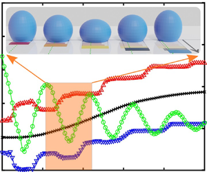



1. Introduction
For millimetric droplets and bubbles with dimensions comparable to the capillary length, phenomena such as coalescence (Yeh et al. Reference Yeh, Fang, Sheen and Yang2013; Soto et al. Reference Soto, Maddalena, Fraters, Van Der Meer and Lohse2018), droplet splitting (Chiou, Chang & Wu Reference Chiou, Chang and Wu2008), oscillation (Duncombe et al. Reference Duncombe, Erdem, Shastry, Baskaran and Böhringer2012), bouncing (Reyssat, Pardo & Quéré Reference Reyssat, Pardo and Quéré2009) and directional transport (Chaudhury & Whitesides Reference Chaudhury and Whitesides1992) under surface gradients are dominated by surface tension forces. Among droplet dynamic actuation and interactions between liquids and solid surfaces, the directional transport of micrometre- and millimetre-sized liquid droplets has attracted considerable interest in the past two decades and offered potential benefits in many applications such as chemical analysis and bioassay systems (Velev, Prevo & Bhatt Reference Velev, Prevo and Bhatt2003; Srinivasan, Pamula & Fair Reference Srinivasan, Pamula and Fair2004; Wixforth et al. Reference Wixforth, Strobl, Gauer, Toegl, Scriba and Guttenberg2004; De Angelis et al. Reference De Angelis, Gentile, Mecarini, Das, Moretti, Candeloro, Coluccio, Cojoc, Accardo and Liberale2011), dropwise condensation heat transfer (Daniel, Chaudhury & Chen Reference Daniel, Chaudhury and Chen2001; Macner, Daniel & Steen Reference Macner, Daniel and Steen2014), water harvesting (Zheng et al. Reference Zheng, Bai, Huang, Tian, Nie, Zhao, Zhai and Jiang2010) and self-cleaning (Blossey Reference Blossey2003).
To control droplet transport on solid surfaces, the interplay and tuning of the different surface tensions involved, i.e. solid–liquid,  $\gamma _{{SL}}$, liquid–vapour,
 $\gamma$, and solid–vapour,
 $\gamma _{{SV}}$, are paramount. One of the common methodologies exploited for droplet manipulation is to create a single sharp contrast (He & Lee Reference He and Lee2003; Kita et al. Reference Kita, Dover, Askounis, Takata and Sefiane2018; Zhao et al. Reference Zhao, Orejon, Mackenzie-Dover, Valluri, Shanahan and Sefiane2020) or a continuous/stepwise gradient (Shastry, Case & Böhringer Reference Shastry, Case and Böhringer2005, Reference Shastry, Case and Böhringer2006; Yang et al. Reference Yang, Chen, Huang and Yeh2006; Reyssat et al. Reference Reyssat, Pardo and Quéré2009; Launay et al. Reference Launay, Sadullah, McHale, Ledesma-Aguilar, Kusumaatmaja and Wells2020) on the solid by adjusting the surface roughness on an intrinsically hydrophobic background, either imposed by the material itself or upon a subsequent coating. In the last century, the influence of roughness on static wetting has been investigated and has been shown to obey the theories of Wenzel (Reference Wenzel1936) or Cassie & Baxter (Reference Cassie and Baxter1944) depending on the intrinsic wettability, the structure of the solid surface and the nature of the liquid. On an intrinsically hydrophilic surface, roughness induces a better wetting behaviour because complete penetration of the liquid into the micro-structures occurs, thus causing an increase in the solid–liquid interfacial area (Kim, Moon & Kim Reference Kim, Moon and Kim2016). This is known as the Wenzel state with a consequent enhanced droplet adhesion (Wenzel Reference Wenzel1936). On an intrinsically hydrophobic surface, roughness results in a lower wettability as a consequence of the suppression of liquid penetration into the micro-/nano-structures and leads to the presence of air pockets, which effectively reduce the droplet–surface interactions. This is known as the Cassie–Baxter state, in which droplets are more mobile (Cassie & Baxter Reference Cassie and Baxter1944). Therefore, introducing a roughness gradient on intrinsically hydrophobic surfaces has been proposed as an effective method to facilitate droplet transport.
With an aim to control droplet motion purely via structural roughness on an intrinsically hydrophobic background, many studies have focused on the design of structured surfaces via micro-fabrication, where the degree of roughness and hence the surface wettability gradient can be precisely adjusted. The first droplet migration reported, owing solely to surface roughness, was achieved on a half-flat–half-rough polydimethylsiloxane (PDMS) substrate, where a droplet placed at the boundary migrated towards the flat area, i.e. the more wettable region, which minimised its surface free energy (He & Lee Reference He and Lee2003). Thereafter, the first continuous surface tension gradient stemming from a progressive change in the solid fraction, i.e. surface roughness, was created by Shastry et al. (Reference Shastry, Case and Böhringer2005, Reference Shastry, Case and Böhringer2006). In their work, they proposed a model that accounted for the hysteresis force to be overcome for the migration of the droplet to ensue, which was thereafter validated by experimental observations (Shastry et al. Reference Shastry, Case and Böhringer2006). At the same time, spontaneous droplet motion was achieved on a micro-grooved surface by adjusting the solid fraction of the grooves to impose the necessary driving force for the motion (Yang et al. Reference Yang, Chen, Huang and Yeh2006). By examining hysteresis more closely, it was found that among the surface topography and structural length scale effects, discontinuous segments, such as micro-pillars, influenced hysteresis the most (Öner & McCarthy Reference Öner and McCarthy2000). Specifically, more irregular micro-pillar shapes, such as rhombuses or stars, induce higher hysteresis than smoother contoured shapes. Further, the critical angles for the onset of droplet sliding on tilted surfaces were compared among surfaces with different micro-structural shapes, namely micro-pillars and micro-grooves, and for the latter, in both groove and orthogonal directions (Yoshimitsu et al. Reference Yoshimitsu, Nakajima, Watanabe and Hashimoto2002). The smallest sliding angles, thus lowest hysteresis, were observed for droplet motion on micro-grooved surfaces, i.e. micro-striated surfaces, along the striation direction.
Other works have proposed physical principles relating friction or hysteresis to the micro-structure solid fraction (Xu & Choi Reference Xu and Choi2012; Kita et al. Reference Kita, Dover, Askounis, Takata and Sefiane2018), and driving force or velocity to the solid fraction gradient (Kita et al. Reference Kita, Dover, Askounis, Takata and Sefiane2018), by considering the droplet–surface interactions and the droplet shape as a linear and continuous gradient between the initial and the final positions. More recently, Zhao et al. (Reference Zhao, Orejon, Mackenzie-Dover, Valluri, Shanahan and Sefiane2020) proposed a unified criterion where it is described that the droplet motion, as displacement, and average velocity are solely functions of the structural parameters of the micro-striated surfaces,  $D, \bar {v}\propto \Delta \phi / \bar {\phi }$. However, on a superhydrophobic, micro-structured surface, droplets typically do not experience steady motion, especially in the initial stages when they first contact or spread on the surface (Bartolo, Josserand & Bonn Reference Bartolo, Josserand and Bonn2005; Yang et al. Reference Yang, Chen, Huang and Yeh2006; Jung & Bhushan Reference Jung and Bhushan2008; Reyssat et al. Reference Reyssat, Pardo and Quéré2009; Wildeman et al. Reference Wildeman, Visser, Sun and Lohse2016; Kita et al. Reference Kita, Dover, Askounis, Takata and Sefiane2018; Gordillo, Riboux & Quintero Reference Gordillo, Riboux and Quintero2019; Launay et al. Reference Launay, Sadullah, McHale, Ledesma-Aguilar, Kusumaatmaja and Wells2020). Although most works on droplet motion on micro-structured surfaces have reported the presence of an oscillatory behaviour (Yang et al. Reference Yang, Chen, Huang and Yeh2006; Kita et al. Reference Kita, Dover, Askounis, Takata and Sefiane2018; Launay et al. Reference Launay, Sadullah, McHale, Ledesma-Aguilar, Kusumaatmaja and Wells2020; Zhao et al. Reference Zhao, Orejon, Mackenzie-Dover, Valluri, Shanahan and Sefiane2020) even when the droplet is deposited gently on the surface, the influence of such oscillatory behaviour on the droplet motion has not been further pursued or investigated. The existence of oscillations has an important influence on droplet behaviour and has been used to realise droplet motion even without a wettability gradient/contrast by surface vibration (Brunet, Eggers & Deegan Reference Brunet, Eggers and Deegan2007; Shastry, Taylor & Bohringer Reference Shastry, Taylor and Bohringer2007; Noblin, Kofman & Celestini Reference Noblin, Kofman and Celestini2009).
One of the first works on the oscillatory behaviour of (free) droplets controlled by surface tension is attributable to Lord Rayleigh (Reference Rayleigh1879). Oscillations caused by a small distortion from the equilibrium shape were investigated much later in different circumstances such as in large electric fields (Morrison, Leavitt & Wortman Reference Morrison, Leavitt and Wortman1981) or in gaseous environments upon break-up from a liquid jet (Becker, Hiller & Kowalewski Reference Becker, Hiller and Kowalewski1991). Some theoretical works (Courty, Lagubeau & Tixier Reference Courty, Lagubeau and Tixier2006; Chevy et al. Reference Chevy, Chepelianskii, Quéré and Raphaël2012) have provided models of the droplet oscillation on non-wetting substrates, where the oscillation period was investigated. To understand the interaction between vertical oscillation and horizontal migration, a determination of the behaviour of the contact line (CL) is essential; however, none of the theoretical works mentioned previously investigated the behaviour of the CL under the influence of oscillations. The simulation work of Lyubimov, Lyubimova & Shklyaev (Reference Lyubimov, Lyubimova and Shklyaev2006) investigated free and forced oscillations of a hemispherical droplet on substrates with different conditions of the CL (free or pinned). On hydrophobic, micro-structured surfaces comprising a wettability contrast, the simulation work of Moradi, Varnik & Steinbach (Reference Moradi, Varnik and Steinbach2010) captured the oscillatory behaviour of the CL. However, no theoretical model to date has yet been proposed to describe the free oscillatory motion of droplets and the CL on micro-structured surfaces. Further, to date, the lack of knowledge of the interactions between the oscillatory motion and the unidirectional migration remains.
The purpose of this work is to propose a more complete, dynamic picture of the motion of a droplet on a hydrophobic surface under the influence of surface wettability contrast, inertia, friction and hysteresis. First, this study will experimentally investigate whether droplets can experience a horizontal migration, a vertical oscillatory motion as well as an alternating leading and trailing motion of the CL. Second, a dynamic physical model will be developed to explain the phenomena observed, where the vertical oscillatory motion and the horizontal migration have been coupled. Subsequently, the model will be compared with the experimental observations.
2. Materials and methods
The solid surfaces used to investigate the spontaneous droplet motion across a contrasting wettability boundary were hydrophobic striated micro-structures. It is noted here that we define a boundary as the intersection between the regions of the solid micro-structured surface with different solid fraction parameters, which is different from the conventional definition of interfacial boundary widely used in the fields of hydrodynamics and fluid mechanics. Parallel, geometric striations, of a top-hat profile, were etched via the deep reactive-ion etching (the Deep-RIE or Bosch process) (Laermer & Schilp Reference Laermer and Schilp1996) onto smooth silicon wafers with a pre-designed mask, which led to an excellent spatial resolution of the motifs, as may be seen in the micrograph of figure 1. Different levels of wettability were achieved by imposing different geometric parameters, i.e. different solid fractions or, expressed alternatively, different ratios of the top solid surface area to the whole projected surface area, between structural units with a well-defined boundary. All micro-striations were of constant height, h, equal to  $20\ \mathrm {\mu }\textrm {m}$, but with different values of width, w, and spacing, s. The solids fabricated offered a wide range of solid fractions,
 $\phi$, defined as
 $\phi =w/(w+s)$. Surfaces with
 $\phi$ varying from 0.10 to 0.91 were produced. Following Deep-RIE and further cleaning, the surfaces were coated with a perfluorodecyltrichlorosilane (FDTS) monolayer that imposed homogeneous intrinsic hydrophobicity on the micro-striated structures (see appendix A.1 for fabrication details). Wettability on both micro-striated and flat FDTS-coated surfaces was characterised by measuring the apparent,
 $\theta _{{app}}$, advancing,
 $\theta _{{adv}}$, and receding,
 $\theta _{{rec}}$, contact angles (CAs). CAs were measured using a Drop Shape Analyser 100 (DSA 100, Krüss GmbH, Hamburg, Germany) and are given in table 1 (see appendix A.2 for detailed information on CA measurements). Droplets of distilled water with a volume of approximately
 $9\ \mathrm {\mu }\textrm {l}$ (corresponding to a droplet radius upon deposition below the capillary length for water, this latter being approximately 2.7 mm) were gently deposited at the boundary of two contrasting micro-striated surfaces (see appendix A.2 for detailed information on droplet volume). Experimental observations of the droplet motion were recorded with a high-speed camera (Chronos 1.4, Kron Technologies Inc., Canada) at 1000 fps and subsequently analysed with a custom-made MATLAB® code.
Scanning electron microscopy (SEM) image showing the structure at the boundary of micro-striations on the surface with  $w=10\ \mathrm {\mu }\textrm {m}$,
 $s=90\ \mathrm {\mu }\textrm {m}$
 $(\phi _{L}=0.10)$ on the left and
 $w=10\ \mathrm {\mu }\textrm {m}$,
 $s=40\ \mathrm {\mu }\textrm {m}$ (
 $\phi _{R}=0.20$) on the right. Inset shows magnification at the micro-striation boundary. Geometrical parameters h, w and s are included in the inset for clarity.

Characteristics of the geometric parameters of the micro-structure, width, w, spacing, s, and solid fraction,  $\phi$, and the contact angles (CAs) of water on each of the surface units. Here
 $\theta _{{app}}$,
 $\theta _{{adv}}$ and
 $\theta _{{rec}}$ are the apparent, advancing and receding CAs of water on each surface unit. All CAs were measured in the orthogonal direction to the micro-striations (Zhao et al. Reference Zhao, Orejon, Mackenzie-Dover, Valluri, Shanahan and Sefiane2020).

3. An example of droplet dynamic motion
A representative example of droplet motion across the boundary of two contrasting units, specifically, left unit ( $\phi _{L}=0.10$) and right unit (
 $\phi _{R}=0.20$), is shown in figure 2(a). The dynamic CAs along with the positions of the centre of mass (c.m.) in the horizontal (x) and vertical (y) directions, and the contact points (CPs), which are extracted from the custom-built MATLAB® code, are plotted in figures 2(b) and 2(c), respectively. CPs are defined as the front (right) and rear (left) points of the CL in the direction of the motion along the micro-striations, as can be seen in the side view in figure 2(a).
(a) Sequential photographs of a  $9\ \mathrm {\mu }\textrm {l}$ droplet moving on the boundary of unit 1 (
 $\phi _{L}=0.10$) and unit 2 (
 $\phi _{R}=0.20$). Parts of the period of motion (5–20, 60 and 100 ms) and the final position (145 ms) with displacement, D, of the centre of mass (c.m.) from the initial position to the instantaneous position are presented. The green dots represent the c.m. of the droplet and the horizontal dotted line shows the position of the boundary on the surface, which are clearly visible in the last photo (at 145 ms). (b) Right (red) and left (blue) dynamic CAs of the droplet versus time. Note that the sudden drop of the left CA at approximately 60 ms arises from the completion of the CL motion across the boundary. Experimental values of
 $\theta _{{adv}}$ and
 $\theta _{{rec}}$ for each independent unit from table 1 are indicated by the dotted lines for
 $\theta _{{adv}}=158^\circ$ and
 $\theta _{{rec}}=151 ^\circ$ for unit 1 (
 $\phi _{L}=0.10$), and
 $\theta _{{adv}}=151^\circ$ and
 $\theta _{{rec}}=143 ^\circ$ for unit 2 (
 $\phi_R=0.20$). (c) Horizontal motion of left and right contact points (CPs) and c.m., and vertical oscillation of the c.m. with time. Green/yellow shaded stripes marked in
 $(b{,}c)$ indicate the downward/upward motion periods of c.m., y. Arrows in
 $(c)$ indicate the corresponding axis for each curve.

After deposition at the contrasting boundary, the droplet undergoes horizontal motion (c.m., x) towards the right surface unit as a result of the imposed wettability contrast and consequently the unbalanced wetting and dewetting behaviours of the CL as the system attempts to minimise its overall surface free energy. In addition to its horizontal motion, the droplet simultaneously experiences rapid damping of the oscillations occurring in the vertical direction (c.m., y), at an initial oscillation period of approximately 20 ms, as shown in figure 2(c). This oscillatory behaviour, in turn, influences the dynamic CAs as well as the behaviour of the CPs in figures 2(b) and 2(c), respectively. Just after deposition, from time  $t = 0\ \textrm {ms}$ to
 $t \sim 10\ \textrm {ms}$, the droplet spreads slightly over the surface, with left and right CPs moving away from each other. Thereafter, from
 $t \sim 10$ ms to
 $t \sim 20$ ms, both CPs dewet/recede towards the droplet centre. Photographs taken during this period are shown in figure 2(a). The CPs then continue to oscillate while the droplet migrates in the same direction of the wettability contrast, i.e. towards the right, from
 $t \sim 20$ ms to
 $t \sim 100$ ms, as represented in figures 2(a) and 2(c). The variation in solid fraction across the boundary provides a contrast in wettability and therefore a net force towards the higher solid fraction unit side, which induces the droplet to migrate. From figure 2(b), at approximately 60 ms, the sudden drop of the left CA indicates that the droplet has moved completely across the boundary and finds itself on a uniform, homogeneous section of the substrate, where there is no longer any gradient in wettability, as is clearly shown in figures 2(a) and 2(c). Although no sudden change in the horizontal motion of the c.m. is noticeable after the CL fully moves across the boundary, the driving force induced by the structural gradient now vanishes, and any further droplet motion solely arises from the inertial overshoot until the droplet finally comes to a rest.
Furthermore, when looking closely at figures 2(b) and 2(c), the CPs move synchronously with the vertical oscillation. They move only when the dynamic CAs are found beyond the  $\theta _{{adv}}$ and
 $\theta _{{rec}}$ of the corresponding surfaces that the CPs move on, as indicated by the dashed lines. Otherwise they are pinned owing to hysteresis and insufficient driving force. When the CPs are pinned temporarily (edges of each shaded stripe), the oscillation leads to deformation of the droplet shape near the CPs and, therefore, the consequent rapid changes in the dynamic CAs, until the CPs start to advance/recede again. When the CPs move (middle of each shaded stripe), the dynamic CAs change is less pronounced, when compared with the case of pinned CPs, and their values revolve around the peak/trough values. To determine the interaction between the vertical oscillation and horizontal migration, it is crucial to know how the droplet oscillates and its influence on the CL.
4. Theoretical model
To explain the dynamics of the oscillatory motion as well as the final position of the droplet with respect to the solid wetting boundary, we have developed and coupled simple mathematical models. Before the droplet leaves the boundary, its motion can be regarded as the superposition of two components: vertical damped oscillation and horizontal migration. As a preliminary step, we model a liquid spheroid to describe the vertical oscillatory motion observed. Subsequently, we refine the full spheroid model to a truncated spheroid, which allows us to connect the vertical motion with the horizontal CL behaviour. The CL behaviour is asymmetric, owing to the different wettability imposed across the boundary, and is further accounted for in the alternating CL slipping model. Finally, a horizontal migration model that takes into account the vertical oscillation, friction and CL hysteresis is presented to explain the droplet motion even after it has moved completely across the wettability boundary.
4.1. Vertical oscillatory model
From figure 2(a), at deposition  $t = 0 \ \textrm {ms}$, the shape of the droplet deviates slightly from sphericity. Because the most energetically favourable shape for a liquid droplet (in the absence of gravity) is that of a sphere (or spherical cap, when in contact with a solid), any deviation/deformation from sphericity will increase its overall free energy. The energy increase associated with deformation causes the tendency to return to spherical symmetry, but inertia leads to an overshoot and an oscillatory cycle is established. Consider the left-hand sketch of figure 3(a), where a prolate spheroid of volume
 $V_{s}$ is a reasonable approximation to the deformed drop at this stage. The radius,
 $a_{s}$, of the equivalent
 $spherical$ droplet is given by
 \begin{equation} a_{s}=\sqrt[3]{\frac{3V_{s}}{4{\rm \pi}}}. \end{equation}
(a) Schematic diagram of droplet evolution in the oscillatory model and (b) corresponding photographs of motion in figure 2(a) between  $t = 0\ \textrm {ms}$ and
 $t = 20\ \textrm {ms}$.

During vertical oscillation, to a reasonable approximation, the droplet modelled by a spheroid changes its shape from prolate ( $\varepsilon > 0$) to oblate (
 $\varepsilon < 0$) with an alternate positive to negative perturbation in the vertical position of the c.m.,
 $\varepsilon$. Therefore, the polar radius of the prolate (subscript
 $p$) or oblate (subscript
 $o$) is
 $a_{{p,o}}=a_{{s}}+ \varepsilon$. The time-dependent polar radius,
 $a$, i.e. the vertical position of the c.m. of the spheroid, can be then expressed as (see detailed derivation in Appendix B):
 \begin{equation} a=a_{s}+\varepsilon(t)=a_{s}+A\exp{\left(-\frac{Ht}{2m}\right)} \cos{\left(\sqrt{\frac{16{\rm \pi}\gamma}{5m}-\frac{H^2}{4m^2}}\cdot t+\beta\right)}. \end{equation}
Here A is the amplitude of the oscillation, H is a dissipation coefficient, m is the mass of the droplet,  $\gamma$ is the surface tension of the water–air interface and
 $\beta$ is the phase angle at
 $t = 0$. The initial condition when the droplet is released from the needle is
 $\beta =0$. Equation (4.2) also includes the oscillation period,
 $\tau$:
 \begin{equation} \tau=2{\rm \pi}\left(\frac{16{\rm \pi}\gamma}{5m}-\frac{H^2}{4m^2} \right)^{-{1}/{2}}. \end{equation}
Clearly a full spheroid would only contact the solid substrate, a plane, at one point. To incorporate a CL of finite length into the model, a truncated spheroidal shape must be used. Consider a truncated sphere of radius of curvature,  $a_{{ts}}$, contact radius,
 $r_{{ts}}$, and distance from the centre to the truncation plane,
 $y_{{ts}}$, as in figure 4 middle.
Truncated spheroids, representing a liquid drop, at three different stages: prolate spheroid (left), sphere (middle) and oblate spheroid (right).

By assuming a constant volume condition and  $a_{{ts}}=a_{{s}}$ for the truncated spheroid during shape change, the relation between the whole and the truncated spheroid can be derived (see detailed derivation of (C5) in Appendix C):
 \begin{equation} y=y_{{ts}}(a_{{ts}}+\varepsilon)/a_{{ts}}, \end{equation}
where y is the vertical height above the solid of the centre of the truncated prolate spheroid ( $\varepsilon > 0$), sphere (
 $\varepsilon =0$,
 $y=y_{{ts}}$) or oblate spheroid (
 $\varepsilon < 0$) and
 $\varepsilon$ is derived in (4.2). The base radius, r, can be written as (see detailed derivation of (C6) in Appendix C):
 \begin{equation} r\approx r_{{ts}}\left(1-\frac{\varepsilon}{2a_{{ts}}}\right), \end{equation}
which allows us to follow the change of r with  $\varepsilon$. The value of r is not constant during the oscillation. In addition, when the droplet contacts the solid surface, to further account for the influence of hysteresis during the oscillation, we have
 $y(t)$ (see detailed derivation of (C8) in Appendix C):
 \begin{equation} y(t) = y_{{ts}}+A'\exp{\left(-\frac{Ht}{2m}\right)} \cos{\left(\sqrt{\frac{16{\rm \pi}\gamma}{5m}(1+{h})-\frac{H^2}{4m^2}}\cdot t+\beta\right)}, \end{equation}
where  $A'=A y_{{ts}}/a_{{ts}}$ and h is a hysteresis coefficient (the details of its expression can be found in Appendix C).
However, with these models, we still cannot describe the asymmetrical behaviour of the left (subscript  $L$) and right (subscript
 $R$) parts of the CL, henceforth denoted as
 $CL_L$ and
 $CL_R$, respectively. The hydrophobicity and hysteresis are different for the two units across the boundary, so when the droplet oscillates vertically on the boundary,
 $CL_L$ and
 $CL_R$ experience different forces, which accounts for the horizontal migration of the droplet. We must therefore develop an alternating CL slipping model to account for the different forces at
 $CL_L$ and
 $CL_R$ and relate the horizontal migration of the droplet to the driving force and resistance from the micro-structure units across the boundary.
4.2. Alternating CL slipping model
Slippage of the CL is an essential ingredient in our description of droplet bouncing and migration across the wetting boundary. However, the mathematics in three dimensions becomes intractable and therefore we present a simplified two-dimensional model here, which adopts the assumption of a drop of unit thickness, as shown in the inset of figure 6. Before the droplet finally leaves the boundary entirely (after approximately 60 ms), the left and right CAs increase and decrease synchronously, although the difference between their values is typically only a few degrees, as shown in figure 2( $b$). We take
 $\theta$ to be the dynamic CA, at a given instant, for both
 $CL_L$ and
 $CL_R$. The apparent equilibrium CAs on respectively the left and the right unit surfaces alone are denoted as
 $\theta _{{L}}^*$ and
 $\theta _{{R}}^*$. These apparent CAs differ from those on an ideal (flat), solid surface of the same chemical constitution, i.e. from the Young's CA,
 $\theta _{{Y}}$ (Young Reference Young1805), which follows the Cassie–Baxter relation (Cassie & Baxter Reference Cassie and Baxter1944):
 \begin{equation} \cos{\theta_{{L,R}}^*} =\phi_{{L,R}}(1+\cos{\theta_{{Y}}})-1. \end{equation}
Adopting in the nomenclature  $F_{L}$ and
 $F_{R}$ to represent the forces acting at
 $CL_L$ and
 $CL_R$ (see the inset of figure 6):
 \begin{gather} F_{{L}}={-}\phi_{{L}}(\gamma_{{SV}}-\gamma_{{SL}} )_{{L}}+\gamma(1-\phi_{{L}})+\gamma\cos{\theta} ={-}\gamma(\cos{\theta_{{L}}^*}-\cos{\theta}), \end{gather}
 \begin{gather}F_{{R}}=\phi_{{R}}(\gamma_{{SV}}-\gamma_{{SL}} )_{{R}}+\gamma(1-\phi_{{L}})-\gamma\cos{\theta} = \gamma(\cos{\theta_{{R}}^*}-\cos{\theta}). \end{gather}
We consider first the case of the c.m. moving in the downwards direction (green stripes, e.g. between  $t = 0\ \textrm {ms}$ and
 $t = 10\ \textrm {ms}$ in figure 2b,c). It is quite plausible that for some time
 $\theta > \theta _{{L}}^* > \theta _{{R}}^*$, hence
 $\cos {\theta } < \cos {\theta _{{L}}^*} < \cos {\theta _{{R}}^*}$, and it follows that
 $| F_{L}| < | F_{R}|$. The time-dependent apparent CA,
 $\theta (t)$, can then be expressed as
 \begin{equation} \theta(t)=\theta_{{L}}^*+\delta(t)=\theta_{{R}}^*+\delta(t)+\xi \end{equation}
where  $\xi$ is a small, positive constant (
 $\xi =\theta _{{L}}^*-\theta _{{R}}^*$, the intrinsic difference between
 $\theta _{{L}}^*$ and
 $\theta _{{R}}^*$) and
 $\delta (t)$ is small and a function of time, t. The forces acting at
 $CL_L$ and
 $CL_R$ can be written as
 \begin{gather} F_{{L}}(t) \approx{-}\gamma\sin{\theta_{{L}}^*}\cdot \delta(t), \end{gather}
 \begin{gather}F_{{R}}(t) \approx \gamma\sin{\theta_{{R}}^*}\cdot (\xi+\delta(t)). \end{gather}
Note that  $\delta (t)$ is positive at this stage. There will be some resistance to motion of the CLs,
 $\varPsi _{L}$ and
 $\varPsi _{R}$ for the left and right surface, respectively, which may be interpreted as wetting hysteresis. If
 $\delta (t)$ is sufficiently large to satisfy the condition:
 \begin{equation} \varPsi_{L} < |\gamma\sin{\theta_{{L}}^*}\cdot\delta(t)|, \varPsi_{R}< |\gamma\sin{\theta_{{R}}^*}\cdot (\xi+\delta(t))|, \end{equation}
then both  $CL_L$ and
 $CL_R$ move. This corresponds to the situation observed just following droplet deposition. Thereafter, as damping of the oscillations takes place (between
 $t \sim 30$ ms and
 $t \sim 60$ ms in figure 2b,c), there is a period when
 \begin{equation} |\gamma\sin{\theta_{{L}}^*}\cdot\delta(t)| <\varPsi_{L}, \varPsi_{R} < |\gamma\sin{\theta_{{R}}^*}\cdot (\xi+\delta(t))|, \end{equation}
and  ${CL_L}$ is anchored by hysteresis whereas
 ${CL_R}$ slips/advances to the right under a force of
 $||\gamma \sin \theta _{{R}}^**(\xi +\delta (t))|-\varPsi _{R}|$, which results in slight movement of the c.m. to the right, as shown in figure 5a2,a3). As the droplet oscillation loses amplitude, for
 $t > 100\ \textrm {ms}$ in figure 2(b),
 $\delta (t)$ decreases and we attain the state where
 \begin{equation} |\gamma\sin{\theta_{{R}}^*}\cdot (\xi+\delta(t))|<\varPsi_{R}, \end{equation}
whereby both  $CL_L$ (now moves across the boundary) and
 $CL_R$ become anchored (permanently), i.e.the motion comes to an end. For
 $CL_L$ in the non-overshooting case,
 $|\gamma \sin {\theta _{{L}}^*}\cdot \delta (t)| <\varPsi _{L}$.
(a) Schematic diagram of evolution of droplet shape and position in the oscillatory truncated model. Colour bars show the length and position of footprints in different states. (b) Sequential photographs of a  $9\ \mathrm {\mu }\textrm {l}$ droplet moving on the boundary of unit 1 (
 $\phi _{L}=0.10$) and unit 2 (
 $\phi _{R}=0.20$) for comparison. Dotted lines indicate the position of the contrast boundary.

We now consider the upward phase of oscillation, when  $\delta (t)$ decreases (yellow stripes, e.g. between
 $t\sim 10$ ms and
 $t \sim 20$ ms in figure 2
 $b$,
 $c$). This implies that
 $\theta _{{L}}^* > \theta _{{R}}^*>\theta$, and we have
 $| F_{L}(t)| > | F_{R}(t)|$ (provided
 $\xi$ is sufficiently small). Then, (4.11) and (4.12) remain valid but note that
 $\delta (t)$ is now negative, which implies that
 $F_{L}(t)$ acts towards the right. Thereafter, there is a period (e.g. between
 $t \sim 30$ ms and
 $t \sim 60$ ms in figure 2b,c) when
 \begin{equation} \varPsi_{L}<|\gamma\sin{\theta_{{L}}^*}\cdot\delta(t)|,|\gamma\sin{\theta_{{R}}^*}\cdot (\xi+\delta(t))|<\varPsi_{R}, \end{equation}
for which  ${CL_R}$ is anchored whereas
 $CL_L$ slips towards the right (as shown in figure 5a4,a5) under the force
 $||\gamma \sin \theta _{{L}}^**\delta (t)| - \varPsi _{L} |$. As the droplet contacts the structured solid surface, the CLs move synchronously during the upward and downward oscillatory phases and the tendency for the c.m. of the droplet to move to the right-hand side is weak. However, at the later stages, when damping has become significant, in both cases,
 $| F_{L}(t)| < \varPsi _{L}$ and
 $| F_{R}(t)| < \varPsi _{R}$, both
 $CL_L$ and
 $CL_R$ are pinned, and the droplet stops moving. Between the onset and the final damping of the droplet motion, there is a stage when
 $CL_L$ and
 $CL_R$ move alternately towards the right, so the main displacement of the c.m. takes place between
 $t \sim 30$ ms and
 $t \sim 60$ ms in figure 2(b) and 2(c). In addition, after the droplet has moved totally across the boundary and before it stops (between
 $t \sim 60$ ms and
 $t \sim 100$ ms in figure 2(b) and 2(c), there is a stage when the droplet overshoots for a further distance beyond the boundary. During this stage, the inertia of the c.m. of the droplet is sufficient to pull
 $CL_L$ and to push
 $CL_R$ so that the behaviours of both
 $CL_L$ and
 $CL_R$ remain virtually unchanged as the droplet slides over the boundary until the droplet comes to a rest at the last stage of the migration.
4.3. Horizontal migration model
Once the droplet has left the boundary, it cannot move indefinitely because the droplet footprint is completely on a homogeneous micro-striated unit, i.e. in the absence of a wettability contrast, and therefore in the absence of a driving force. Motion is here then limited to that arising from inertia. (Momentum was neglected in the preceding argument, owing to it being of secondary importance, but once the CLs become symmetrical, on the same solid surface texture, this becomes the overriding effect.) Returning to the more realistic three-dimensional model, the net surface force acting on the droplet sitting on the boundary in the  $x$ direction with the centre position at
 $x_{o}$ (as shown in figure 6) is
 \begin{gather} F_{{d}}=2|\int_{\omega_{{o}}}^{\rm \pi}\gamma(\cos{\theta_{{R}}^*}-\cos{\theta_{{L}}^*} )\cos{\omega}rd\omega|=2\gamma r\sin{\omega_{{o}}}\Delta\cos{\theta^*}\nonumber\\ =2r\sqrt{1-(x_{o}/r)^2}\gamma\Delta\cos{\theta^*}, \end{gather}
where  $\Delta \cos {\theta ^*} = \cos {\theta _{{R}}^*} - \cos {\theta _{{L}}^*}$,
 $r$ is the droplet contact radius and
 $\omega _{o}$ is the azimuthal angle corresponding to half of the droplet footprint arc on the right-hand side of the boundary, equal to
 $\omega _{o} = {\rm \pi}- \cos ^{-1}{x_{o}/r}$. We assume that the resistance to motion from the surface,
 $f_{L,R}$, is directly proportional to the solid/liquid contact area (the assumption of
 $f_{L,R} \propto R^2$ in the present case is reasonable as the comparison of the calculated velocity by the model with experimental results provides a better agreement than for the case where the resistance is dominated by the CL,
 $f_{L,R} \propto R$):
 \begin{gather} f_{L}=2\left|\int_{{-}r}^{{-}x_{o}}B\phi_{L}\sqrt{r^2-x^2}\,{\textrm{d}x}\right|=2\gamma B^*\phi_{L}r\int_{x_{o }/r}^{1}\sqrt{1-(x/r)^2}d(x/r), x \leq r, \end{gather}
 \begin{gather}f_{R}=2\left|\int_{{-}x_{o}}^{r} B\phi_{R}\sqrt{r^2-x^2}\,{\textrm{d}x}\right|=\gamma B^*\phi_{R}r\left({\rm \pi}-2\int_{x_{o }/r}^{1}\sqrt{1-(x/r)^2}d(x/r)\right), x \leq r, \end{gather}
where  $B$ is a coefficient accounting for friction (assumed to be independent of the solid surface motif),
 $B^*$ is normalised
 $B$ by surface tension,
 $\gamma$, and droplet contact radius,
 $r$, and equals
 $B^*=Br/\gamma$. After moving across the boundary, i.e. when
 $x_{o} > r$, we have
 $F_{d}= 0$,
 $f_{L}=0$ and
 \begin{equation} f_{R} = \gamma {\rm \pi}r B^* \phi_{R}, x > r. \end{equation}
To obtain information about the speed, the work done by the forces from (4.17)–(4.20) needs to be calculated. Assuming the normalised displacement of the c.m.,  $x$, by the droplet contact radius,
 $r$,
 $x^* = x/r < 1$, and integrating the forces from
 $x^* = 0$ to
 $x^* = x_{o}^* = x_{o}/r$, the work done by the above-mentioned driving force and left and right friction forces are
 $W_{F_{d}}(x_{o}^*)$,
 $W_{f_{L}}(x_{o}^*)$ and
 $W_{f_{R}}(x_{o}^*)$, respectively, which can be derived as (
 $x_{o}^* < 1$)
 \begin{gather} W_{F_{d}}(x_{o}^*)=\int_{0}^{x_{o}} F_{d}\,{\textrm{d}x} = 2 \gamma r^2 \Delta \cos{\theta^*} \int_{0}^{x_{o}^*}\sqrt{1-(x^*)^2}\,{\textrm{d}x}^*, \end{gather}
 \begin{gather}W_{f_{L}}(x_{o}^*) = \int_{0}^{x_{o}} f_{L}\,{\textrm{d}x} =r \int_{0}^{x_{o}^*} f_{L}\,{\textrm{d}x}^*, \end{gather}
 \begin{gather}W_{f_{R}}(x_{o}^*) = r \int_{0}^{x_{o}^*} f_{R}\,{\textrm{d}x}^*. \end{gather}
When  $x_{o}^* > 1$, the works become
 $W_{F_{d}}(x_{o}^*) = W_{F_{d}}(1)$,
 $W_{f_{L}}(x_{o}^*) = W_{f_{L}}(1)$ and
 \begin{equation} W_{f_{R}}(x_{o}^*) = W_{f_{R}}(1)+ \gamma B^* \phi_{R} {\rm \pi}r^2 (x_{o}^*-1). \end{equation}
The contributions from the initial deposition and CL pinning to the kinetic energy must also be taken into account. The vertical oscillation and the droplet horizontal shift are related in the alternating CL slipping model. Further vertical oscillation helps the droplet to overcome hysteresis, therefore, leading to a larger horizontal kinetic energy. Furthermore, experiments demonstrated that for cases with large hysteresis, at the end of the motion, the droplet wobbled horizontally, with its CL pinning onto the surface before becoming still. This suggests that the inertia force cannot overcome the pinning of the CL and part of the kinetic energy is dissipated without enabling the droplet to move further. In consideration of all the above-mentioned effects, the kinetic energy,  $E$, involved in the droplet migration on a striated surface comprising a structural wetting gradient at a given normalised displacement from the boundary,
 $x_{o}^*$, is given by
 \begin{equation} E(x_{o}^*)=W_{D}(x_{o}^*) + W_{F_{d}}(x_{o}^*) - W_{f_{L}}(x_{o}^*) - W_{f_{R}}(x_{o}^*) - W_{H}(x_{o}^*)=\tfrac{1}{2} m v^2, x_{o}^* <1, \end{equation}
where  $v$ is the droplet velocity and
 $W_{{D}}(x_{o}^*)$ is the net kinetic energy converted from a vertical oscillation. The oscillation results in a forced wetting/dewetting behaviour of the CL, which is asymmetric along the motion direction, and contributes to the value of
 $E$ even without a wettability gradient (Dong, Holmes & Böhringer Reference Dong, Holmes and Böhringer2017). In the present case, the asymmetry of the wetting/dewetting behaviour is solely caused by the surface morphology, which vanishes once the droplet moves across the boundary, and
 $W_{{D}}(x_{o}^*)$ does not contribute further to the kinetic energy. Here
 $W_{{H}}(x_{o}^*)$ is the kinetic energy dissipated after the CL is pinned and before the droplet comes to a final halt. Owing to the existence of hysteresis, the CL stops moving prior to the droplet, and the droplet starts ‘wobbling’ under the ‘extra’ kinetic energy,
 $W_{{H}}(x_{o}^*)$, which has no contribution to the droplet motion. For the overshoot cases,
 $E(1) > 0$, which means when the whole footprint leaves the boundary, the kinetic energy of the droplet is non-zero, which drives the droplet to move further from the boundary. For non-overshoot cases,
 $E(x_{m}^* )=0$, where the maximum normalised displacement,
 $x_{m}^* < 1$, which means the kinetic energy dissipates totally before the droplet leaves the boundary.
Schematic diagram of the droplet footprint across the boundary of the wettability contrast with a displacement  $x_{o}$. The origin, O, is set to be the centre of the footprint contacted with the solid surface, which moves with the droplet. Inset shows the directions of the surface forces acting on the
 $CL_L$ and
 $CL_R$.

According to (B7) in Appendix B,  $W_{{D}}(x_{o}^*)$ should be a function of the change in potential energy, upon gentle deposition, from the initial deposition state to the equilibrium state, as
 $W_{{D}}(x_{o}^*) \propto 8{\rm \pi} \gamma \varepsilon _{{m}}^2/5$, where
 $\varepsilon _{{m}}$ is the maximum position change of the c.m.,
 $y$ and
 $\varepsilon _{{m}} \propto a_{{ts}}-y_{{ts}}$. Moreover, the kinetic energy converted from the vertical oscillation contributes to both sides of the CL motion; therefore, the increased driving force in the direction of the droplet motion should be a function of the difference in the projected length of the CL in the perpendicular direction in a similar fashion to (4.17) and (4.21). Then,
 $W_{{D}}(x_{o}^*)$ is expressed as
 \begin{equation} W_{D}(x_{o}^*) = C \frac{8 {\rm \pi}\gamma (a_{{ts}}-y_{{ts}})^2}{5} \int_{0}^{x_{o}^*}\sqrt{1-(x^*)^2}\, {\textrm{d}x}^*, \end{equation}
where  $C$ is a factor accounting for the proportion of the energy converted from the total vertical mechanical energy by the droplet shape oscillation.
The hysteresis term,  $W_{{H}}(x_{o}^*)$, appears only when the motion comes to its end. From the experimental results, we found a continuity of the kinetic energy declining to zero instead of a sudden drop when the CL was finally pinned. In addition, in some cases, we were even able to see a slight horizontal wobbling of the c.m. when CL was pinned. We also noticed that on the surface with higher
 $\bar {\phi }$, CL was pinned more easily and the velocity declined at a faster rate. To take into account this part of the energy and satisfy the kinetic energy continuity, we assume
 \begin{equation} W_{H}(x_{o}^*) \propto Z \left(\frac{x_{o}^*}{x_{m}^*}\right)^{k}, \end{equation}
where  $k$ is a factor indicating how fast
 $W_{{H}}(x_{o}^*)$ reaches to its maximum when
 $x_{o}^*$ gets close to
 $x_{m}^*$, whereas
 $Z$ is the portion of kinetic energy that would be dissipated after CL is finally pinned, which can be derived by meeting the condition
 $E(x_{m}^*) = 0$. Because
 $k$ is related to hysteresis, we assume
 $k=1+\bar {\phi }$, where
 $\bar {\phi } = (\phi _{{L}} + \phi _{{R}})/2$, the average fraction of the given micro-striated surfaces across the boundary. By solving (4.17)–(4.27), the velocity of the motion,
 $v$, can be estimated as a function of the position, while the maximum displacement
 $x_{m}^*$ is attained from the experimental results. An example of the evolution of each term involved in (4.25) as a function of
 $x_{o}^*$ is shown in figure 11.
5. Comparison of experimental results and theory
First, we compare the vertical oscillation and the truncated models to the experimental results for a wide range of solid fraction difference between striations in figure 7. For the results related to the smallest solid fraction difference between striations, i.e. the cases closest to a homogeneous striated surface in the absence of contrast in the solid fraction, there is a good agreement between the experimental and the model results are achieved. We note here that the oscillatory behaviour on homogeneous surfaces could further support the theoretical model; however, the static nature of the droplets without the motion in the horizontal direction bring such considerations beyond the purpose of this work. The evolution of the contact radius  $r$ and the height of the droplet centroid (
 $y$) for both experiments (subscript
 $e$) and models (subscript
 $m$) for five different cases are shown in figure 7. The best fit for
 $k_h$ in Appendix C is
 $k_h\approx 1.8$ and the dissipation coefficient,
 $H$, is
 $H\approx 0.35\times 10^{-3}\ \textrm {kg}\,\textrm {s}^{-1}$. For a
 $9\ \mathrm {\mu }\textrm {l}$ water droplet with
 $m = 9 \times 10^{-6}\ \textrm {kg}$ and
 $\gamma = 72\ \textrm {mN}\,\textrm {m}^{-1}$, and neglecting the dissipation term, the angular frequency can be estimated as
 $\omega \approx \sqrt {16{\rm \pi} \gamma /(5m)}$ and the oscillation period, as shown in figure 7(
 $a$), is thus
 $\tau \approx 2{\rm \pi} \sqrt {5m/(16{\rm \pi} \gamma )} = 22\ \textrm {ms}$, which is in good agreement with our experimental results, at least in the initial stage (
 $\tau \approx 20\ \textrm {ms}$). In addition, in the same magnitude, by making use of the Rayleigh equation (Rayleigh Reference Rayleigh1879), a free droplet gives
 $\tau \approx 2{\rm \pi} \sqrt {m/(8{\rm \pi} \gamma )} = 14\ \textrm {ms}$.
(a–e) Comparison of experimental (subscript  $e$) and model (subscript
 $m$) results for the vertical oscillation of the c.m., y (mm), and contact radius, r (mm), with elapsed time t (ms) for five different cases. The left and right surface fractions are shown in each graph, e.g. (
 $\phi _{L}=0.10$) and unit 2 (
 $\phi _{R}=0.20$) in (a). Examples of initial amplitude,
 $A$, and initial oscillation period,
 $\tau$, from the model are shown in (
 $a$). (f) Dependence of oscillation period on
 $\bar {\phi }$ for all the experimental cases (red circles) with the result predicted by the model (black line).

Initially, the droplet oscillates with a large amplitude, which suggests that the local, instantaneous variations in Laplace pressure near the CL, caused by distortion of the droplet from spherical, are sufficient to overcome wetting hysteresis and thus prompt outward/inward motion of the CL. Later, as the oscillations become damped as a consequence of energy dissipation, Laplace pressure variations are no longer sufficient to overcome hysteresis. When comparing the theoretical and experimental results of the vertical oscillations of the c.m., it can be seen that the model captures the oscillations quite well. When the c.m. is moving downwards/upwards, the CL is forced to spread/retract and the contact radius increases/decreases. There is a good agreement of the oscillation period between the theoretical and experimental results. In figure 7(f), the model captured the dependence of the oscillation period on  $\bar {\phi }$, where the period decreases with
 $\bar {\phi }$. The droplets on surfaces with higher
 $\bar {\phi }$ experience higher degree of hysteresis, as per the higher solid fraction. Therefore, the CL is pinned more easily during the oscillation, which forces the droplet to oscillate faster until it reaches the equilibrium state, and leads to a lower oscillation period. For the contact radius, there is a rather good qualitative agreement: the droplet spreads and recedes alternately. It is noteworthy that there is a large quantitative discrepancy of the contact radius in figure 7(a,e). In the case of figure 7(a), the oscillation behaviour is strongest and the droplet overspreads onto the surface, which lead to not only a larger oscillation amplitude of the CL but also a larger value of the final contact radius than expected, because the droplet cannot restore its profile to an equilibrium state owing to hysteresis especially when its CL is receding. In the case of figure 7(e), in the presence of a large
 $\Delta \phi$, the droplet experiences greater deviations from the spherical shape, i.e.droplet elongation, owing to the preferential spreading onto the right-hand side, which results in the deviation of the contact radius. In the assumption of the model, the distortion of the shapes from equilibrium should be small. An oscillation with a larger amplitude or an elongated shape leads to a bigger deviation between the theoretical and experimental results, mainly in the values of the amplitude, whereas the oscillation of the period are rather well captured. In our earlier work (Zhao et al. Reference Zhao, Orejon, Mackenzie-Dover, Valluri, Shanahan and Sefiane2020), the effect of the amplitude on the horizontal migration/displacement by releasing the droplet from certain heights was found to increase with increasing the releasing height, i.e. Weber number, within a certain range. This work, however, aims to minimise the influence of the deposition on the reported amplitude, which has proven to be challenging to accurately adjust, so further investigation of the effect of the amplitude on the horizontal migration/displacement by releasing the droplet from certain heights is proposed as the scope for future work.
Just after deposition, the droplet swells in the lower part, owing to a downwards momentum transfer. This increases the local curvature, thus generating a stronger momentary Laplace pressure than for a perfect oblate spheroid, which drives the CL to expand more on the surface than predicted by the model. Thereafter, momentum transfer leads to more liquid in the upper part than in the lower part (figure 2( $a$) at
 $t = 25\ \textrm {ms}$). The reduced volume in the lower part hence reduces the local curvature and a lower Laplace pressure permits the CL to move inwards more than in the case of a perfect prolate spheroid. For the case of a larger
 $\phi _{{R}}$, as shown in figure 7(
 $c$–
 $e$), with higher degrees of both wettability and hysteresis, it is more difficult for the CL to shrink, which results in a larger radius. Such perturbations in droplet shape, which are not allowed for in the model, can probably explain, at least to some extent, the reason for the quantitative differences seen between the experimental and model contact radii of the droplet in figure 7. With the increase of
 $\bar {\phi }$, the gap between the two results diminishes, because on surfaces with larger
 $\phi$, the droplet spreads more before it detaches from the needle, and the vertical oscillation becomes weaker as a consequence of the enhanced droplet–surface affinity. Other parameters that contribute to the differences between model and experimental results could lie in the preferable spreading in the striation direction and the gravity effect. Despite these differences, the model describes, in reasonable qualitative and quantitative detail, the vertical oscillatory motion of the c.m. and the lateral alternate leading and trailing motion of the CL.
In figure 8, the experimental results for droplet velocity,  $v$, versus normalised position with respect to the contact radius,
 $x^*=x/r$, are presented, together with the behaviour expected from the model developed previously. Compared with the experimental results for maximum displacement, the best fits for the coefficients,
 $B^*$ and
 $C$ (in (4.18), (4.19) and (4.26)), are proposed as
 $B^* \approx 18.07\ \textrm {N}\,\textrm {m}^{-2} \cdot r \Delta \phi /\gamma \bar {\phi }$,
 $C\approx 0.13$. In our previous work (Zhao et al. Reference Zhao, Orejon, Mackenzie-Dover, Valluri, Shanahan and Sefiane2020), the average velocity of the droplet, v, is a function of
 $\Delta \phi /\bar {\phi }$,
 $\bar {v} \approx \gamma (\cos {\theta _{Y}}+1)\Delta \phi /(2 \xi \bar {\phi })$, where
 $\xi$ is a friction coefficient. Thus, here,
 $B \propto \bar {v}$.
Comparison of the results of droplet velocity, v  $(\textrm {mm}\,\textrm {s}^{-1})$, versus relative position,
 $x^*$, from the experimental results (data points) and model (trend lines) for five different cases. The contrasting boundary between two units is included within the legend where the numbers on the left and right represent the solid fractions for the left and right units, respectively.

From figure 8, good agreement is found between the experimental results and the proposed model. The model describes well how the velocity changes during droplet motion on a structured surface comprising wettability contrast. The droplet c.m. accelerates rapidly at the initial stage, when the driving force is considerably larger than the resistance to motion. Later, when the droplet moves towards the more hydrophilic unit, i.e. a surface with larger  $\phi _{R}$, according to (4.16), the length of the boundary covered by the droplet decreases; therefore, the driving force decreases whereas the sum of
 $f_{L}$ and
 $f_{R}$ increases. A maximum is reached, followed by deceleration until the drop comes to a halt. The difference between the experimental and model results may arise partially from the assumption that
 $C$ is considered to be a constant, whereas the different amplitude and period of the oscillations of both
 $r$ and
 $y$, the different magnitude of the change in droplet shape caused during deposition and the different droplet surface interactions as a consequence of the different wetting contrast may suggest otherwise. For example, in figure 7, the magnitude of the oscillation as well as the initial contact radius are different for the cases (
 $a$)
 $\phi _{L} = 0.10$,
 $\phi _{R} = 0.20$ and (
 $b$)
 $\phi _{L} = 0.40$,
 $\phi _{R} = 0.50$.
We have further collapsed all experimental cases to investigate the dynamic velocity evolution of droplets moving across the wettability contrast by normalising the velocity and the displacement by the maximum velocity  $v_{m}$ and maximum displacement
 $x_{m}$ of each wetting contrast configuration, respectively. The results are presented in figure 9(
 $a$).
 $(a)$ Experimental cases are collapsed by normalising the velocity and the displacement by the maximum velocity,
 $v_{m}$, and the maximum displacement,
 $x_{m}$, of each wetting contrast configuration, respectively. The theoretical model of the case 0.10–0.20 is added for comparison.
 $(b)$ Comparison of the integral function
 $F(x_{o}^*)$ derived from experimental values of the dynamic velocity for all wetting contrast configurations and from the theoretical model, where
 $x_{o}^*$ is a given displacement normalised by the droplet contact radius,
 $r$. The droplet moves across the boundary at
 $x_{o}^*=1$.

Figure 9 shows that droplets first accelerate upon contacting the surface, then reach the maximum velocity when the driving force and resistance are balanced, and then decelerate until they stop. To understand the evolution of the driving force for all the different cases regardless of the surface parameters, we present all experimental cases in figure 9( $b$) by re-arranging (4.17)–(4.25) and simplifying some terms (see appendix E).
 $F(x_{o}^*)$ in figure 9(
 $b$) is then an indicator of the contribution of the driving force to the kinetic energy as a function of the normalised displacement. Good agreement can be found especially in the early stage. The theoretical value of
 $F(x_{o}^*)$ at
 $x_{o}^*=1$, where the droplet moves across the boundary, is found to be
 $F(1)={\rm \pi} /4\approx 0.79$. For the cases where the droplet can reach
 $x_{o}^*=1$, the experimental value of
 $F(1)$ varies between 0.6 and 0.9. The error mainly comes from two sources. One arises from the fact that
 $W_{D}(x_{o}^*)$ is neglected, then the contribution of the deposition is included into
 $W_{F_{d}}(x_{o}^*)$, so
 $F(x_{o}^*)$ is larger than expected. However, because
 $W_{H}(x_{o}^*)$ is neglected, the energy dissipated after CL pinning is not included, which leads to a smaller
 $F(x_{o}^*)$. Clear evidence for this is that, for some cases, where the droplet stops before it moves across the boundary totally (
 $x_{o}^*=1$), the experimental curve of
 $F(x_{o}^*)$ deviates greatly from the theoretical curve and stops because the velocity becomes 0. Therefore, the term
 $W_{H}(x_{o}^*)$ can no longer be neglected in the cases where the droplet is not able to move fully across the boundary.
6. Conclusion
The dynamic behaviour of a droplet moving across the boundary of a wettability contrast micro-structured surface has been experimentally observed and analysed. After being deposited on the boundary, the droplet experiences a vertical damped oscillation and, simultaneously, a horizontal migration. The vertical oscillatory model presented in § 4.1 and the alternating CL slipping model presented in § 4.2 have been developed and coupled to explain the relation between vertical and horizontal motion as well as the behaviour of the CL. In addition, the horizontal migration aspect has been coupled with the vertical oscillation to describe the migration velocity of the droplet in the horizontal migration model presented in § 4.3. The coupling of all three models provides good agreement with the experimental results, which describe the velocity and position of a droplet deposited at a structural contrasting boundary as it migrates towards a denser structured unit. It is noteworthy that not all the cases exhibit a complete droplet migration across the boundary, although both the overshooting and non-overshooting cases have been analysed and captured by the model. Further application of the complete models should enable good prediction of the detailed motion of droplets moving on wetting contrast surfaces or surfaces with wetting contrasts placed in sequence. This is of importance for the optimisation and accurate design of micro-fluidic devices.
Acknowledgements
The authors would like to acknowledge the support of Dr C. Mackenzie-Dover and the Scottish Microelectronics Centre (SMC) for substrate micro-fabrication and surface coating.
Funding
The authors would like to acknowledge the support of the European Space Agency (ESA) through the project Convection and Interfacial Mass Exchange (EVAPORATION) with ESA Contract Number 4000129506/20/NL/PG. The authors also acknowledge the support received from the Engineering and Physical Sciences Research Council (EPSRC) through the grant EP/P005705/1.
Declaration of interests
The authors report no conflict of interest.
Appendix A. Details on experiment and measurements
A.1. Surface fabrication
Four-inch silicon wafers were purchased from Si-Mat (Silicon Materials, Landsberg, Germany). Hexamethyldisilizane (HMDS) was applied to the wafer as an adhesive for the photoresist for 10 min. Silicon wafers were used without a further cleaning procedure as any additional dry or wet cleaning treatment may have induced further deposition of dirt and/or contaminants. Then, the wafers were placed in an SVG 8600 (Silicon Valley Group, USA) track system to dispense and spin coat a SPR 350 photoresist layer with a thickness of  $1.2\ \mathrm {\mu }\textrm {m}$ onto the surfaces. Following this, the wafers and the photoresist were soft-baked on a heating plate at
 $90\,^{\circ }\textrm {C}$ for 60 s, exposed for 5 s in a vacuum inside a Karl Suss MA8 mask aligner (Süss, Garching, Germany) and further developed inside the SVG 8600. The substrates were then covered by a pre-designed mask displaying the desired micro-structure patterns and were then exposed to UV light through the mask. After the development process, the exposed resist was washed away, which left the patterned resist on the substrates. The substrates were then subjected to deep reactive-ion etching (deep-RIE, Bosch process) in a surface technology system STS Multiplex ICP (inductively coupled plasma). Etching was carried out for 20 cycles. After etching, the resist was removed from the substrate by acetone, which left the rigid micro-structures with a height of
 $20\ \mathrm {\mu }\textrm {m}$ on the substrates. The surface fabrication was carried out within the Class 10 cleanrooms of the Scottish Microelectronic Centre (SMC). After fabrication, the substrates were sealed in a wafer box and sent to Memsstar Ltd., Scotland for coating. A monolayer of FDTS was applied onto the substrates, which made the surface micro-structures intrinsically hydrophobic.
A.2. Experimental measurements
CA measurements were conducted on the Drop Shape Analyser 100 (DSA 100, Krüss GmbH, Hamburg, Germany) platform. The apparent CA of the droplet,  $\theta _{{app}}$, was measured in both the parallel and orthogonal directions to the micro-striations upon gentle deposition. The
 $\theta _{{app}}$ measured in the orthogonal direction was found to be dependent on the micro-striation parameters, and the values for different surface units are listed in table 1. The advancing and receding CAs,
 $\theta _{{adv}}$ and
 $\theta _{{rec}}$, were measured in the orthogonal direction by adding and withdrawing liquid, respectively, which are listed in table 1. The standard error was estimated from five independent measurements with a system accuracy of
 $0.3^{\circ }$. We note here that the standard error for all cases was within
 $3^{\circ }$.
The standard error in the volume of the deposited droplets from five independent measurements and calculations via image processing was estimated as approximately  $0.5 \ \mathrm {\mu } \textrm {l}$. The deviation of the volume resulted from the difficulty to deposit a water droplet onto hydrophobic surfaces with a low solid fraction, i.e. superhydrophobic surfaces. When the volume is small, it is difficult for the water droplet to detach from the needle owing to the low adhesion between the droplet and the hydrophobic surface, and when the volume is large, the surface tension cannot always hold the dosed droplet as a whole, which leaves a small part of the droplet attached to the needle; hence the dosage volume will be less than expected.
Furthermore, the presence of the anisotropic micro-striations induces, to some extent, preferential spreading of the droplet along the striation direction rather than in the orthogonal direction. The anisotropic deviation of the droplet shape was noted by the use of a top view camera, and the difference of droplet radii measured along the two directions was estimated to be within about 7 %.
Appendix B. Derivation details on vertical oscillation of a spherical droplet
As stated in (4.1), the radius,  $a_{s}$, of the equivalent
 $spherical$ droplet is given by
 \begin{equation} a_{s}=\sqrt[3]{\frac{3V_{s}}{4{\rm \pi}}}, \end{equation}
where  $V_{s}$ is the volume of the spheroid. The spherical droplet changes its shape from prolate (
 $\varepsilon >0$) to oblate (
 $\varepsilon <0$) with an alternate positive to negative perturbation in the vertical position of c.m.,
 $\varepsilon$. Therefore, the polar radius of the prolate (subscript
 $p$) or oblate (subscript
 $o$) is
 $a_{p,o}=a_{s}+\varepsilon$. The equatorial radius of the spheroid,
 $b_{p}$ or
 $b_{o}$ is given by
 \begin{equation} b_{p,o}=\sqrt{\frac{3V_{s}}{4{\rm \pi} (a_{s}+\varepsilon)}} =\sqrt{\frac{a_{s}^3}{a_{s}+\varepsilon}}. \end{equation}
To evaluate the free energy of the droplet associated with its surface, the surface area of the equivalent spheroid,  $S_{p,o}$, is required. The surface area for a prolate spheroid,
 $S_{p}$, is given by (Weisstein Reference Weisstein2003c)
 \begin{equation} S_{p}=2 {\rm \pi}b_{p}^2\left(1+\frac{a_{p}}{b_{p} e_{p}} \sin^{{-}1}{e_{p}}\right), \end{equation}
where the eccentricity  $e_{p}=\sqrt {1-(b_{p}/a_{p})^2}=\sqrt {1-(a_{s}/(a_{s}+\varepsilon ))^3}$. Using the Maclaurin series expansion (Weisstein Reference Weisstein2003a),
 $S_{p}$ can be written as
 \begin{equation} S_{p} = 2 {\rm \pi}\frac{a_{s}^3}{a_{s}+\varepsilon}\left(1+\sqrt{\frac{(a_{s}+\varepsilon)^3}{a_{s}^3 e_{p}^2}} \sin^{{-}1}{ e_{p}}\right) \approx 4 {\rm \pi}a_{s}^2 \left(1+ \frac{2 \varepsilon^2 }{5 a_{s}^2}\right). \end{equation}
For an oblate spheroid surface,  $S_{o}$ can be written as (Weisstein Reference Weisstein2003b)
 \begin{equation} S_{o}=2 {\rm \pi}b_{o}^2+ {\rm \pi}\frac{a_{o}^2}{e_{o}} \ln{\frac{1+e_{o}}{1-e_{o}}}, \end{equation}
where the eccentricity  $e_{o}=\sqrt {1-(a_{o}/b_{o})^2} = \sqrt {1-((a_{s}+\varepsilon )/a_{s})^3}$. As previously,
 $S_{o}$ can be written as
 \begin{equation} S_{o} \approx 4 {\rm \pi}a_{s}^2 \left(1+ \frac{2 \varepsilon^2 }{5 a_{s}^2}\right). \end{equation}
Thus, to a first approximation, the surface areas of prolate and oblate spheroids, when only slightly deformed, are the same,  $S_{p}=S_{o}$, and given by either (B4) or B6. Neglecting gravity, as is reasonable in the present context, the potential energy,
 $P$, of a perturbed drop is driven by surface tension and thus given by
 \begin{equation} P \approx 4 {\rm \pi}\gamma a_{s}^2 \left(1+ \frac{2 \varepsilon^2 }{5 a_{s}^2}\right), \end{equation}
where  $\gamma$ is the liquid–vapour surface tension of the droplet. The internal kinetic energy of the droplet,
 $K$ , can be defined as
 $K \approx 1/2\;m \dot {\varepsilon }^2$, where
 $m$ is the droplet mass. A more complete analysis allowing for shape change contributions to
 $K$ leads to a pre-factor of 27/40 instead of 1/2, but this leads to undue complication and unwarranted precision (for more details on a more complete analysis, see appendix D). Whereas the internal viscous dissipation,
 $D$, as
 $D \approx 1/2 H \dot {\varepsilon }^2$, where
 $H$ is a dissipation coefficient, may be related to liquid viscosity and/or to the surface structure; nonetheless, for the sake of simplicity, the model assumes a constant value. Further analysis demonstrated that the variability of
 $H$ as a function of
 $\bar {\phi }$ was found to have negligible impact (i.e. a low contribution of one or two orders of magnitude) on predicting the period of oscillations. In light of the agreement obtained between the model and the experiment, this seems to be a reasonable assumption while keeping the model as simple as possible. We construct the Lagrangian function,
 $L$:
 \begin{equation} L=K-P=\frac{1}{2} m \dot{\varepsilon}^2 - 4{\rm \pi}\gamma a_{s}^2 \left(1+ \frac{2 \varepsilon^2 }{5 a_{s}^2}\right). \end{equation}
The corresponding Lagrange equation of the first kind with respect to the dynamic deviation from sphericity,  $\dot {\varepsilon }$, is
 \begin{equation} \frac{\textrm{d}}{\textrm{d}t}\left(\frac{\partial L}{\partial \dot{\varepsilon}}\right) -\frac{\partial L}{\partial \varepsilon}+\frac{\partial D}{\partial \dot{\varepsilon} }=0. \end{equation}
 \begin{equation} m \ddot{\varepsilon}+ H \dot{\varepsilon} +\frac{16 {\rm \pi}\gamma \varepsilon}{5}=0. \end{equation}
Solving (B10), we obtain the time-dependent deviation of the polar radius of the spheroid,  $\varepsilon (t)$:
 \begin{equation} \varepsilon(t)= A\exp{\left(-\frac{Ht}{2m}\right)}\cos{\left(\sqrt{\frac{16{\rm \pi}\gamma}{5m}-\frac{H^2}{4m^2}}\cdot t+\beta\right)}. \end{equation}
And the time-dependent polar radius of the spheroid,  $a(t)$, is
 \begin{equation} a(t) = a_{s}+\varepsilon(t)=a_{s}+A\exp{\left(-\frac{Ht}{2m}\right)} \cos{\left(\sqrt{\frac{16{\rm \pi}\gamma}{5m}-\frac{H^2}{4m^2}}\cdot t+\beta\right)}. \end{equation}
Appendix C. Derivation details on vertical oscillation of a truncated spherical droplet
The volume of a truncated sphere,  $V_{ts}$, is given by
 \begin{equation} V_{ts}=\int_{{-}y_{ts}}^{a_{ts}}{\rm \pi} x^2\,{\textrm{d}y} =\frac{\rm \pi}{3}(2 a_{ts}^3 +3 a_{ts}^2 y_{ts} - y_{ts}^3) =\frac{\rm \pi}{3}a_{ts}^3 (1-\cos{\theta^*})^2 (2+ \cos{\theta^*}), \end{equation}
where  $\theta ^*$ (equivalent to the apparent CA of the droplet, but here is simply a geometrical concept) is the interior angle subtended between the tangent to the spheroid and the truncation plane at their intersection and
 $y_{ts}=-a_{ts}\cos {\theta ^*}$. The base radius of a truncated sphere (contact radius of the droplet),
 $r_{ts}$, is
 $r_{ts}=a_{ts}\sin {\theta ^*}$.
For a truncated prolate or oblate spheroid shown in figure 4 (left) and (right), respectively, the volume,  $V$, is given by
 \begin{equation} V=\int_{{-}y_{p,o}}^{a} {\rm \pi}b^2 (1-y_{p,o}^2/a^2)\,{\textrm{d}y} = \frac{\rm \pi}{3} b^2 \left(2 a+ 3 y_{p,o} -\frac{y_{p,o}^3}{a^2}\right). \end{equation}
With the constant volume condition:
 \begin{equation} b^2 \left(2 a+ 3 y_{p,o} -\frac{y_{p,o}^3}{a^2}\right)=2 a_{ts}^3 +3 a_{ts}^2 y_{ts} - y_{ts}^3. \end{equation}
By comparing full and truncated spheroids (figures 3 and 4), therefore taking  $a_{ts}=a_{s}$,
 $b=b_{p,o}=\sqrt {a_{s}^3/(a_{s}+\varepsilon })$, we have
 $a=a_{ts}+\varepsilon$ and (C3) becomes
 \begin{equation} a_{ts}^3 \left[2 + \frac{3 y_{p,o}}{a_{ts}+\varepsilon} -\frac{y_{p,o}^3}{(a_{ts}+\varepsilon)^3}\right]=a_{ts}^3\left(2 +\frac{3 y_{ts}}{a_{ts}} - \frac{ y_{ts}^3}{a_{ts}^3}\right). \end{equation}
The real solution of this equation is
 \begin{equation} y_{p,o} = \frac{y_{ts} (a_{ts}+\varepsilon)}{a_{ts}}, \end{equation}
and the base radius,  $r$, can be written as
 \begin{equation} r=b\sqrt{\left(1-\frac{y^2}{a^2}\right)} = b\sqrt{\left(1-\frac{y_{ts}^2}{a_{ts}^2}\right)} \approx a_{ts} \sin{\theta^*} \left(1-\frac{\varepsilon}{2 a_{ts}}\right) = r_{ts} \left(1-\frac{\varepsilon}{2 a_{ts}}\right). \end{equation}
When the droplet contacts the solid with a finite contact area, the CL needs to overcome hysteresis before it can move. Compared with the ideal cases without hysteresis, the existence of hysteresis in the realistic case distorts the droplet shape from the spheroid shape, i.e. part of the kinetic energy is ‘stored’ temporally, which should be a function of the surface area as well as the degree of hysteresis. Accounting for this part of the energy, we introduce another term,  $-hP=- 4{\rm \pi} \gamma a_{s}^2 (1+ {2 \varepsilon ^2 }/{5 a_{s}^2}){h}$, in (B8):
 \begin{equation} L=K-P=\frac{1}{2} m \dot{\varepsilon}^2 - 4{\rm \pi}\gamma a_{s}^2 \left(1+ \frac{2 \varepsilon^2 }{5 a_{s}^2}\right)(1+{h}), \end{equation}
where  $h$ is the coefficient of the stored energy by surface distortion via hysteresis. According to (B12) and (C5), the vertical position of
 $y(t)$ is
 \begin{equation} y(t) = y_{{ts}}+A'\exp{\left(-\frac{Ht}{2m}\right)} \cos{\left(\sqrt{\frac{16{\rm \pi}\gamma}{5m}(1+{h})-\frac{H^2}{4m^2}}\cdot t+\beta\right)}, \end{equation}
where  $A'=A y_{{ts}}/a_{{ts}}$ and the coefficient,
 $h$, should be a function of
 $\bar {\phi }$, which presents the degree of hysteresis, so we assume the expression for
 $h$ is
 ${h}={k_h}\bar {\phi }\gamma$, where
 $\bar {\phi } = (\phi _{{L}} + \phi _{{R}})/2$ and
 ${k_h}$ is set to be a constant for the sake of simplicity of the model. It is noteworthy that the surface distortion term,
 $-{h}P$, only exists when the CL is pinned, and it is released as kinetic energy as soon as the CL moves. From figure 2
 $(c)$, we know that the CL is pinned when
 $\varepsilon ^2$ is at its maxima and moves when
 $\varepsilon ^2$ is small; therefore, for the simplicity of the model, we assume that the distortion term induced by hysteresis continuously changes with
 $\varepsilon ^2$ . Equation (C8) is applied to the derivation of the results in figure 7. It is noteworthy that
 $y(t)$ is the vertical position of the centre of the spheroid above the surface, and the geometric centroid, i.e. the c.m. of the droplet, is above
 $y(t)$ by
 $3/4R(1+\cos {\theta ^*})^2/(2+\cos {\theta ^*})$ (Harris & Stöcker Reference Harris and Stöcker1998). This has been taken into account in
 $y_m$ in figure 7.
Appendix D. Derivation of kinetic energy of the droplet
For the whole spheroid, normalising  $\varepsilon$ by
 $a_{s}$ so
 $\varepsilon ^*=\varepsilon /a_{s}$, we have
 $a_{p,o}=a_{s}+\varepsilon =a_{s}(1+\varepsilon ^*)$, and (B2) becomes
 \begin{equation} b_{p,o}=\sqrt{\frac{a_{s}^3}{a_{s}+\varepsilon}}=a_{s}(1+\varepsilon^*)^{-{1}/{2}}. \end{equation}
Taking the oblate spheroid case in figure 10 as an example ( $\varepsilon <0$), where
 $r_{os}$ represents the radius of the horizontal cross-section circle with a vertical distance from the origin,
 $y$, the distance between a point on the horizontal cross-section circle to the centre of the certain circle,
 $r(y)=\sqrt {x^2+z^2}$, obeys
 $0 \leq r(y) \leq r_{os}(y)$. Using the equation for a vertically axisymmetric ellipsoid,
 $(x^2+z^2)/b^2+y^2/a^2=1$, we have
 \begin{gather} \frac{{r_{os}^2(y)}}{a_{s}^2}(1+\varepsilon^*)+\frac{y^2}{a_{s}^2}(1+\varepsilon^*)^{{-}2}=1, \end{gather}
 \begin{gather}r_{os}^2(y^*) = a_{s}^2\left[\frac{1}{1+\varepsilon^*}+\frac{{y^*}^2}{({1+\varepsilon^*})^3}\right], \end{gather}
where  $y^*=y/a_{s}$. During the vertical oscillation, by homothety, we assume the local vertical velocity inside the spheroid,
 $v_{v}$, increases linearly with height and with the boundary conditions
 $v_{v}=0$, where
 $y=-a$, i.e. the spheroid contacts the wall, and
 $v_{v}=\dot {\varepsilon }$, where
 $y=0$, i.e. the c.m. of the droplet has a vertical velocity
 $\dot {\varepsilon }$. Then the vertical velocity at (
 $y,r$) within the oblate spheroid is
 $v_{v}=\dot {\varepsilon }(1+y/a)=a_{s}\dot {\varepsilon }^*[1+y^*/{(1+\varepsilon ^*)}]$, where
 $\dot {\varepsilon }^*=\dot {\varepsilon }/a_{s}$.
Schematic diagram of the whole oblate spheroid. A random point on the surface is shown in the figure with the coordinates ( $y, r_{os}$). Here
 $r_{os}=\sqrt {x^2+z^2}$, where
 $x$ and
 $z$ are the coordinates along the
 $x$ and
 $z$ axes.

Assume a droplet with a density of  $\rho$ has the same shape as the oblate spheroid, then a disc of thickness
 $a_{s} \delta y^*$ from the droplet has a vertical energy,
 $K_{v}=1/2\delta m v_{v}^2$, of
 \begin{equation} K_{v}(y^*) = {\rm \pi}\rho r_{os}^2 a_{s} \delta y^* \frac{1}{2} v_{v}^2 = \frac{\rm \pi}{2} \rho a_{s}^5 \delta y^* {\dot{\varepsilon}}^{*2} \left[\frac{1}{1+\varepsilon^*}+\frac{{y^*}^2}{({1+\varepsilon^*})^3}\right] \left(1+\frac{{y^*}^2}{1+\varepsilon^*}\right)^2. \end{equation}
Taking  $Y = y^*/(1+\varepsilon ^*)=y/a$ and
 $\delta Y=\delta y /[a_{s} (1+\varepsilon ^*)]$, (D4) becomes
 \begin{equation} K_{v}(Y) = \frac{\rm \pi}{2} \rho a_{s}^5 \delta Y {\dot{\varepsilon}}^{*2} (1-Y^2)(1+Y)^2. \end{equation}
Because  $-1 < Y < 1$, by integrating
 $K_{v}(Y)$ from -1 to 1, the total vertical internal kinetic energy,
 $K_{tv}$, is derived as
 \begin{equation} K_{tv} = \frac{\rm \pi}{2} \rho a_{s}^5 {\dot{\varepsilon}}^{*2} \int_{{-}1}^{1}(1-Y^2)(1+Y)^2 \,\textrm{d} Y=\frac{4}{5} {\rm \pi}\rho a_{s}^5 {\dot{\varepsilon}}^{*2}=\frac{3}{5} m {\dot{\varepsilon}}^{2}, \end{equation}
where  $m$ is the whole mass of the droplet.
Furthermore, there exists a horizontal component of internal  $K$. By homothety, we assume a linear local horizontal velocity inside the spheroid along the cross-section radius direction,
 $v_{h}=\dot {r}_{os}r/r_{os}$, where
 $\dot {r}_{os}$ is the horizontal velocity at
 $r=r_{os}$, i.e. on the cross-section circle at a given
 $y$, which can be derived from (D3):
 \begin{equation} \dot{r}_{os} = \frac{-1+3 {y^*}^2/(1+\varepsilon^*)^2}{2(1+\varepsilon^*)^2 r_{os}} a_{s}^2 \dot{\varepsilon}^* . \end{equation}
Then a disc of thickness  $\delta y = a_{s} \delta y^*$ from the droplet has a horizontal kinetic energy,
 $K_{h}(y^*)$, of
 \begin{equation} K_{h}(y^*) = \int_{0}^{r_{os}} \frac{1}{2} v_{h}^2 2 {\rm \pi}r \rho\,\textrm{d} r \delta y= \frac{{\rm \pi} \rho {\dot{r}_{os}}^2}{r_{os}^2} \int_{0}^{r_{os}} r^3\,\textrm{d}r =\frac{\rm \pi}{4} \rho r_{os}^2 {\dot{r}_{os}}^2 a_{s}\delta y^*. \end{equation}
With (D7),  $K_{h}(Y)$ is
 \begin{equation} K_{h}(Y) =\frac{\rm \pi}{4} \rho r_{os}^2 {\dot{r}_{os}}^2 a_{s}\delta y^* = \frac{\rm \pi}{16 (1+\varepsilon^*)^3}\rho a_{s}^5 {\dot{\varepsilon}}^{*2} ({-}1+3Y^2)^2 \delta Y. \end{equation}
Taking that  $\varepsilon ^* \ll 1$, the total horizontal kinetic energy
 $K_{th}$ is
 \begin{equation} K_{th} = \frac{\rm \pi}{16} \rho a_{s}^5 {\dot{\varepsilon}}^{*2} \int_{{-}1}^{1}({-}1+3Y^2)^2 \,\textrm{d} Y=\frac{1}{10} {\rm \pi}\rho a_{s}^5 {\dot{\varepsilon}}^{*2}=\frac{3}{40} m {\dot{\varepsilon}}^{2}, \end{equation}
then the total internal kinetic energy,  $K$, is
 \begin{equation} K = K_{tv} + K_{th} =\frac{27}{40} m {\dot{\varepsilon}}^{2}. \end{equation}
The derivation of  $K$ is the same for a prolate spheroid with
 $\varepsilon > 0$.
Appendix E. Rearrangement and simplification of the horizontal migration model
To determine the evolution of the driving force for all the different cases, we re-arrange (4.17)–(4.25) and make some simplifications. First, the kinetic energy (4.25) for  $x_{o}^* <1$ is
 \begin{equation} E(x_{o}^*)=W_{D}(x_{o}^*) + W_{F_{d}}(x_{o}^*) - W_{f_{L}}(x_{o}^*) - W_{f_{R}}(x_{o}^*) - W_{H}(x_{o}^*)=\tfrac{1}{2} m v^2, \end{equation}
an example of the contribution of each term in (E1) for the case,  $\phi _{L}=0.10$ and
 $\phi _{R}=0.20$, is shown in figure 11. If we now assume that the only driving force is
 $F_{d}$ and neglect the term
 $W_{D}(x_{o}^*)$ (in most of the cases,
 $W_{F_{d}}(x_{o}^*)/W_{D}(x_{o}^*)>4)$, and because
 $W_{H}(x_{o}^*)$ plays its role mainly near the end of the motion, we arrive at the following simplified energy equation:
 \begin{equation} W_{F_{d}}(x_{o}^*) \approx \tfrac{1}{2} m v^2 + W_{f_{L}}(x_{o}^*) + W_{f_{R}}(x_{o}^*). \end{equation}
By making use of (4.7), (4.17)–(4.19) and (4.21)–(4.23), the integral function  $F(x_{o}^*)$ derived from experimental values of the dynamic velocity can be expressed as
 \begin{equation} F(x_{o}^*) = \frac{W_{F_{d}}(x_{o}^*)}{2{\rm \pi}\gamma r^2 (1+\cos{\theta_{Y}})\Delta \phi} \approx \frac{\frac{1}{2} m v^2 + W_{f_{L}}(x_{o}^*) + W_{f_{R}}(x_{o}^*)}{2{\rm \pi}\gamma r^2 (1+\cos{\theta_{Y}})\Delta \phi}. \end{equation}
We also know that the theoretical expression for  $F(x_{o}^*)$ from (4.21) is
 \begin{equation} F(x_{o}^*) = \int_{0}^{x_{o}^*} \sqrt{1-(x^*)^2} \,{\textrm{d}x}^*. \end{equation}
It is now possible to collapse all experimental data using (E3) and compare the results with the theoretical (E4). It is noteworthy that the only fitting parameter in (E3) is  $B^* \approx 18.07\ \textrm {N}\,\textrm {m}^{-2} \cdot r \Delta \phi /\gamma \bar {\phi }$. We cannot further simplify the expression because of the complicated forms of
 $W_{f_{L}}(x_{o}^*)$ and
 $W_{f_{R}}(x_{o}^*)$. Experimental and model results using (E3) and (E4) are then compared in figure 9
 $(b)$. Because
 $W_{F_{d}}(x_{o}^*)=2{\rm \pi} \gamma r^2 (1+\cos {\theta _{Y}})\Delta \phi F(x_{o}^*)$,
 $F(x_{o}^*)$ acts as an indicator of the contribution of the driving force to the kinetic energy as a function of normalised displacement.
The works done by different forces in the case with  $\phi _{L}=0.10$ and
 $\phi _{R}=0.20$, from 0 to a given displacement,
 $x_{o}^*=x_{o}/r$, where
 $r$ is the contact radius of the droplet. The evolution of each term in (E1) is presented.


 Open access

