





1. Introduction
Suspensions of cohesive materials are ubiquitous in many engineered and environmental systems. The complex process of aggregation, breakup and restructuring, known in sediment transport as ‘flocculation’, is poorly understood and difficult to model (Winterwerp & van Kesteren Reference Winterwerp and van Kesteren2004). A popular approach, inspired by Smoluchowski (Reference Smoluchowski1916, Reference Smoluchowski1918), is the population balance equation (PBE). Also used to model bubble and droplet coalescence and breakup, and reacting flows (e.g. Shaw Reference Shaw2003; Rigopoulos Reference Rigopoulos2007; Ramkrishna & Singh Reference Ramkrishna and Singh2014), the PBE describes the evolution of aggregate size concentration over time and space by an advection equation with source and sink terms accounting for discrete aggregation and breakup events. These terms involve probabilistic and rate-describing kernels which are parameterised to construct low-order models (Ives & Bhole Reference Ives and Bhole1973; Winterwerp Reference Winterwerp1998). Despite growing interest in incorporating boundary layer effects (Penaloza-Giraldo et al. Reference Penaloza-Giraldo, Yue, Hsu, Vowinckel, Manning and Meiburg2025a , Reference Penaloza-Giraldo, Yue, Hsu, Vowinckel, Manning and Meiburgb ), parameterisations are often over-simplified, or agnostic to local flow conditions.
Experimental studies have provided valuable insights into aggregate morphology and population dynamics; however, direct observation of aggregation and breakup events requires high-speed imaging and well-controlled environments, often making such experiments prohibitive. Notably, Saha et al. (Reference Saha, Babler, Holzner, Soos, Lüthi, Liberzon and Kinzelbach2016) captured Lagrangian breakup statistics in quasi-homogeneous isotropic turbulence (HIT), while Hoffman & Eaton (Reference Hoffman and Eaton2023) reported statistics on individual aggregation and breakup events in a humid turbulent flow laden with glass particles. Still, most experimental investigations are limited to single aggregates or simplified flows (Blaser Reference Blaser2000; Dizaji et al. Reference Dizaji, Marshall and Grant2019; Qi et al. Reference Qi, Shin and Coletti2025), and systematic variation of cohesive forces remains challenging (Gans et al. Reference Gans, Pouliquen and Nicolas2020). These difficulties have motivated a growing body of numerical work.
With access to detailed data, particle-resolved simulations have yielded insight into how turbulence intensity, cohesive strength, particle volume fraction and other micromechanical properties influence flocculation in HIT (e.g. Yao & Capecelatro Reference Yao and Capecelatro2021; Zhao et al. Reference Zhao, Pomes, Vowinckel, Hsu, Bai and Meiburg2021; Yu et al. Reference Yu, Balachandar, Smith and Manning2024) and, to a lesser extent, wall-bounded flows (e.g. Afkhami et al. (Reference Afkhami, Hassanpour, Fairweather and Njobuenwu2015), Njobuenwu & Fairweather (Reference Njobuenwu and Fairweather2018), Schutte et al. (Reference Schutte, Portela, Twerda and Henkes2018)). A key contribution in this direction is Babler et al. (Reference Babler2015), who conducted one-way coupled direct numerical simulations (DNSs) of point-like aggregates in various wall-bounded flows and identified two breakup mechanisms: weaker aggregates broke throughout the flow due to local turbulent stresses, whereas stronger aggregates migrated closer to a wall before breaking under stresses induced by mean shear. With a similar numerical approach, Breuer & Almohammed (Reference Breuer and Almohammed2015) investigated a turbulent channel laden with aggregating particles (no breakup) and found that aggregation rates peak near the wall, where collision rates are highest. These findings have been extended by studies that incorporate both aggregation and breakup, however, due to computational limitations at the time, those studies were limited to initial aggregation-dominated transients (Afkhami et al. Reference Afkhami, Hassanpour, Fairweather and Njobuenwu2015; Hærvig et al. Reference Hærvig, Sørensen and Condra2018; Njobuenwu & Fairweather Reference Njobuenwu and Fairweather2018).
To avoid complications from drag modelling (Yu et al. Reference Yu, Balachandar, Smith and Manning2024), the present study employs particle-resolved direct numerical simulations (PR-DNSs) to investigate the aggregation and breakup of cohesive particles suspended in a turbulent channel flow. Despite independent insight into each process, to the best of the authors’ knowledge, no studies demonstrate if aggregation and breakup balanced locally in the wall-normal direction, which would reveal regions of net aggregate production or depletion. We employ a PBE framework, introduced in § 5, to process the simulation results and develop a statistical description of aggregation and breakup in the wall-normal direction. Following bulk considerations in § 6.2, regions of net aggregate production and depletion are identified in both physical and size space in § 6.3, revealing a wall-normal imbalance between aggregation and breakup. We then show that this imbalance is closed by the wall-normal advection of aggregates, giving rise to a conceptual picture of statistical circulation in the joint space of size and wall-normal coordinate. Finally, to clarify the mechanisms driving this circulation, near-wall aggregate breakup is examined in § 6.4 while aggregate orientation, rotation and deformation are quantified in § 6.5.
2. Numerical approach
The fluid phase is governed by the continuity
 \begin{equation} \boldsymbol{\nabla }\boldsymbol{\cdot }\boldsymbol{u} = 0, \end{equation}
and Navier Stokes equations
 \begin{equation} \frac {\partial \boldsymbol{u}}{\partial t} + \boldsymbol{\nabla }\boldsymbol{\cdot }\left (\boldsymbol{u}\boldsymbol{u}\right ) = -\frac {1}{\rho _{\!f}}\boldsymbol{\nabla }\! p + \nu \boldsymbol{\nabla} ^2\boldsymbol{u} + \boldsymbol{f}_{\!\textit{IBM}}, \end{equation}
for an incompressible Newtonian fluid with density
 $\rho _{\!f}$
and kinematic viscosity
 $\nu$
. The fluid velocity at a point
 $\boldsymbol{x} = (x, y, z)$
and time
 $t$
is denoted by
 $\boldsymbol{u}(\boldsymbol{x}, t) = (u, v, w)$
, while
 $p$
denotes the pressure, and
 $\boldsymbol{f}_{\!\textit{IBM}}$
the numerical volume force responsible for the coupling between fluid and particle by means of the immersed boundary method (IBM). The particle linear
 \begin{equation} m_{\!p} \frac {\mathrm{d}\boldsymbol{u}_i^P}{\mathrm{d}t} = \oint _{\varGamma _i}\boldsymbol{\tau }\boldsymbol{\cdot }\boldsymbol{n}_i^P\mathrm{d}A + \boldsymbol{F}_{\!c,i}, \end{equation}
and angular momentum equations
 \begin{equation} I_p\frac {\mathrm{d}\boldsymbol{\omega }_i^P}{\mathrm{d}t} = \oint _{\varGamma _i}\boldsymbol{r}_i^P\times \big (\boldsymbol{\tau }\boldsymbol{\cdot }\boldsymbol{n}_i^P\big )\mathrm{d}A + \boldsymbol{T}_{\!c,i}, \end{equation}
are solved concurrently. Here,
 $\boldsymbol{u}_i^P(t)=(u_i^P, v_i^P, w_i^P)$
and
 $\boldsymbol{\omega }_i^P(t)=(\omega _{x,i}^P,\omega _{y,i}^P,\omega _{z,i}^P)$
are the linear and angular velocities of particle
 $i$
,
 $\varGamma _i$
its surface and
 $\boldsymbol{r}_i^P=\boldsymbol{x}-\boldsymbol{x}_i^P$
is the displacement vector from its centre,
 $\boldsymbol{x}_i^P(t)=(x_i^P,y_i^P,z_i^P)$
. All particles have mass
 $m_{\!p}$
, diameter
 $d$
, density
 $\rho _p$
and moment of inertia
 $I_p=\pi \rho _p d^5/60$
. The hydrodynamic stress tensor
 $\boldsymbol{\tau } = p \unicode{x1D644} + 2\rho _{\!f}\nu \unicode{x1D640}$
with
 $ \unicode{x1D640} = (\boldsymbol{\nabla }\boldsymbol{u} + \boldsymbol{\nabla }\boldsymbol{u}^T ) / 2$
is integrated over
 $\varGamma _i$
, while the contact forces,
 $\boldsymbol{F}_{\!c,i}$
, and torques,
 $\boldsymbol{T}_{\!c,i}$
, act when appropriate.
Importantly included in
 $\boldsymbol{F}_{\!c,i}$
are the cohesion and lubrication forces,
 $\boldsymbol{F}_{\!coh,ij}$
and
 $\boldsymbol{F}_{\!\ell ,ij}$
. In this work,
 $\boldsymbol{F}_{\!coh,ij}$
is modelled using the formulation of Vowinckel et al. (Reference Vowinckel, Withers, Luzzatto-Fegiz and Meiburg2019)
 \begin{equation} \boldsymbol{F}_{\!coh,ij} = \begin{cases} -\dfrac {A_H d}{2\zeta _0 \lambda ^3}\big (\zeta _{ij}^2 - \zeta _{ij}\lambda \big )\boldsymbol{e}_{ij}^P, & 0 \lt \zeta _{ij} \leq \lambda ,\\[11pt] 0, & \mathrm{otherwise}, \end{cases} \end{equation}
which provides a computationally efficient approximation of the short-range attractive forces predicted by the Derjaguin–Landau–Verwey–Overbeek theory of van der Waals (vdW) interactions. Here,
 $\boldsymbol{e}_{ij}^P$
is the unit vector directed from the centre of particle
 $i$
to particle
 $j$
,
 $\zeta _{ij} = \lVert \boldsymbol{x}_i^P-\boldsymbol{x}_j^P\rVert -d$
is the minimum surface-to-surface distance between the pair and
 $\zeta _0$
represents the scale of microscopic surface asperities. The parameter
 $\lambda$
defines the finite range over which the cohesive force is distributed and must be set comparable to the other length scales in the problem to not impose computational constraints, thus
 $\lambda = d/20$
, as in Vowinckel et al. (Reference Vowinckel, Withers, Luzzatto-Fegiz and Meiburg2019), who show that pairwise interactions are relatively insensitive to
 $\lambda$
. The Hamaker constant,
 $A_{\!H}$
, characterises the net short-range adhesion between particles, encapsulating the combined influence of particle and fluid material properties. Interpreted here as an effective value, it may therefore also represent additional adhesive mechanisms beyond vdW interactions alone such as polymer bridging or biofilm-mediated cohesion.
When
 $\zeta _{ij} \leq 2\Delta x$
, the close-range hydrodynamic forces can no longer be resolved in the normal direction. Following Biegert et al. (Reference Biegert, Vowinckel and Meiburg2017) and Vowinckel et al. (Reference Vowinckel, Withers, Luzzatto-Fegiz and Meiburg2019), the unresolved normal lubrication force is modelled as
 \begin{equation} \boldsymbol{F}_{\!\ell ,ij} = \begin{cases} -\frac {3\pi \rho _{\!f} \nu d^2}{8\max (\zeta _{ij}, \zeta _{\textit{min}})}\boldsymbol{g}_{ij} & 0 \lt \zeta _{ij} \leq 2 \Delta x,\\[11pt] 0 & \mathrm{otherwise}, \end{cases} \end{equation}
where
 $\Delta x$
is the isotropic grid spacing,
 $\boldsymbol{g}_{ij} = [(\boldsymbol{u}_i^P - \boldsymbol{u}_j^P)\boldsymbol{\cdot }\boldsymbol{e}_{ij}^P ]\boldsymbol{e}_{ij}^P$
is the relative normal velocity between the two particles and
 $\zeta _{\textit{min}} = 1.5\times 10^{-3}d$
is a regularising constant calibrated by Biegert et al. (Reference Biegert, Vowinckel and Meiburg2017).
The cohesion and lubrication forces are accompanied by normal and tangential collision forces,
 $\boldsymbol{F}_{\!n,ij}$
and
 $\boldsymbol{F}_{\!t,ij}$
. Accumulated, the contact forces and torques acting on particle
 $i$
are
 \begin{equation} \boldsymbol{F}_{\!c,i} = \boldsymbol{F}_{\!\ell ,iw} + \boldsymbol{F}_{\!n,iw} + \boldsymbol{F}_{\!t,iw} + \sum _{j,j\neq i}\left (\boldsymbol{F}_{\!\ell ,ij} + \boldsymbol{F}_{\!n,ij} + \boldsymbol{F}_{\!t,ij} + \boldsymbol{F}_{\!coh,ij}\right )\!, \end{equation}
and
 \begin{equation} \boldsymbol{T}_{\!c,i} = \frac {d}{2}\boldsymbol{e}_{iw}^P\times \boldsymbol{F}_{\!t,iw} + \sum _{j,j\neq i}\frac {d}{2}\boldsymbol{e}_{ij}^P\times \boldsymbol{F}_{\!t,ij}, \end{equation}
where the definitions above extend to interactions between particle
 $i$
and wall
 $w$
following Biegert et al. (Reference Biegert, Vowinckel and Meiburg2017), with the exception of the cohesive force, which acts only between particles, consistent with this work’s focus on the dynamics of suspended aggregates rather than their capture by walls. The collision and lubrication models, also adopted in Vowinckel et al. (Reference Vowinckel, Withers, Luzzatto-Fegiz and Meiburg2019), were calibrated against experiments in Biegert et al. (Reference Biegert, Vowinckel and Meiburg2017) so that collision kinematics and a restitution coefficient of
 $0.97$
are well reproduced.
3. Physical configuration
A channel of size
 $(L_x, L_y, L_z) = (6h, 2h, 3h)$
, half-height
 $h$
, is filled with a Newtonian fluid laden with
 $N = 3841$
(volume fraction
 $\phi = N \pi d^3 / (6 L_x L_y L_z) = 0.015$
) cohesive particles of diameter
 $d=2h/31$
and density ratio
 $\rho _s = \rho _p / \rho _{\!f} = 1$
, cf. Figure 1. The streamwise (
 $x$
) and spanwise (
 $z$
) directions are periodic while no-slip walls are imposed at
 $y=0$
and
 $y=2h$
. An adaptive pressure gradient maintains a constant bulk velocity
 $U$
and Reynolds number
 $\textit {Re}=U h / \nu = 2800$
, which, when formulated with the friction velocity
 $u_\tau = \sqrt {\tau _w / \rho _{\!f}}$
and wall shear stress
 $\tau _w$
, corresponds to the well-studied friction Reynolds number of
 $\textit {Re}_\tau = u_\tau h / \nu = 180$
of Kim et al. (Reference Kim, Moin and Moser1987). The domain is discretised using a cubic mesh with grid spacing
 $\Delta x = h/186$
so that the characteristic length scale at the wall, the viscous unit
 $\delta _\nu = \nu / u_\tau$
, is sufficiently resolved:
 $\delta _\nu / \Delta x = 0.9678$
. The particle boundary layers are also resolved, even those at the extreme ends of aggregates. To verify this we follow the procedure detailed in Appendix A to compute the effective slip velocity between particle
 $i$
and the fluid,
 $\Delta \boldsymbol{u}_i^{PF}$
, and subsequently the particle Reynolds number,
 $\textit {Re}_{\!p,i} = \lVert \Delta \boldsymbol{u}_i^{PF}\rVert d / \nu$
. Over all cases,
 $\max _i \textit {Re}_{\!p,i} \leq 49.58$
, so the minimum particle boundary layer is estimated to be
 $\min _i \delta _{\!p,i} \approx d / \sqrt {\max _i\textit {Re}_{\!p,i}} = 1.65\delta _\nu$
and is therefore resolved. Furthermore, the particle resolution of
 $d / \Delta x = 12$
matches past IBM-based PR-DNS studies in turbulent channel flow at a minimum of
 $\textit {Re}_\tau = 180$
(Costa et al. Reference Costa, Brandt and Picano2020; and references therein). It should also be noted that the ratio of particle diameter to Kolmogorov length scale is large in this work, with
 $d / \eta \approx 6.78$
at
 $y = 0.06h$
and
 $d / \eta \approx 3.15$
at the centreline on average. While
 $\eta$
is appropriately resolved, the implications of the particle size are discussed in the conclusion. Lastly, validation for a single-phase and cohesionless suspension is discussed in § 4, with detailed validation of the hydrodynamics and collision schemes against experimental observations reported in Biegert et al. (Reference Biegert, Vowinckel and Meiburg2017), to excellent agreement. Further convergence analysis and comparison with empirical and theoretical settling velocities for single- and multi-sphere aggregates at particle Reynolds numbers up to
 $\textit{Re}_p = 100$
can be found in Vowinckel et al. (Reference Vowinckel, Withers, Luzzatto-Fegiz and Meiburg2019) and Maches et al. (Reference Maches, Houssais, Sauret and Meiburg2024).
Schematic of the simulation domain. Slices from
 $\textit{Co}=1$
are shown sequentially along the channel for increasing times, with aggregates coloured by the number of constituent particles. A corresponding video from case
 $\textit{Co}=0.48$
can be found in the supplementary movie is available at https://doi.org/10.1017/jfm.2026.12202.

Figure 1. Long description
A 3D schematic of a simulation domain showing the evolution of particle aggregates over time. The domain is divided into slices along the channel, with each slice representing a different time point. Aggregates are colored by the number of constituent particles, ranging from light blue for fewer particles to dark blue for more particles. The time points are labeled as t = 0, t = 50, t = 100, t = 150, t = 200, and t = 250. The x, y, and z axes are labeled, and the dimensions of the domain are indicated as 3h, 6h, and 2h.
The cohesive force, (2.5), is characterised by the cohesive number
 \begin{equation} \textit{Co} = \frac {\max \lVert \boldsymbol{F}_{\!coh,ij}\rVert }{\rho _{\!f} U^2d^2}, \end{equation}
which quantifies the ratio of maximum cohesive force to a characteristic particle inertial force. In order to observe measurable aggregation for the present particle size and
 $\textit {Re}$
we select
 $\textit{Co} = \{0, 0.24, 0.48, 1.0, 1.5\}$
. As mentioned in § 2, given the limitations on particle size in PR-DNS, the Hamaker constant should be interpreted as an effective constant; taking the properties of water,
 $\nu = 1.002\times 10^{-6}\,\mathrm{m}^2\,\mathrm{s}^{-1}$
and
 $\rho _{\!f} = 1000\,\mathrm{kg\,m}^{-3}$
, and a surface asperity scale of
 $\zeta _0 = 0.2\,\mathrm{nm}$
(Israelachvili Reference Israelachvili1992), yields
 $A_H = \mathcal{O}(10^{-16}\mathrm{-}10^{-15})\,\mathrm{J}$
, whereas
 $A_H = \mathcal{O}(10^{-20}\mathrm{-}10^{-18})\,\mathrm{J}$
for materials such as quartz in water (Bergström Reference Bergström1997; Marshall & Li Reference Marshall and Li2014).
Particles are initially distributed randomly, without overlap, throughout a fully developed single-phase channel flow, with each particle assigned the mean linear and angular velocities of the replaced fluid. At time
 $t=0$
the particles are released and the simulations are marched forward, allowing particles to aggregate, fragment and redistribute in the turbulent flow. The fluid is advanced using a time step
 $\Delta t_f$
that is continuously adapted so that the Courant number,
 $\mathcal{C}$
, satisfies the Courant–Friedrichs–Lewy condition,
 $\mathcal{C} \leq 0.5$
. Particle kinematics are evaluated using a sub-stepping routine with time step
 $\Delta t_p = \Delta t_f / 15$
. In the spatio-temporal schematic of figure 1, the domain is partitioned into six temporal segments along the streamwise direction to illustrate aggregate growth.
4. Validation
4.1. Single-phase validation
The particle-laden flow is initialised from a fully developed single-phase turbulent channel flow with a measured
 $\textit {Re}_\tau = 179.82$
. For validation, the wall-normal profiles of the mean velocity,
 $\overline {u}^+$
and velocity fluctuations,
 $\overline {u'u'}^+$
,
 $\overline {v'v'}^+$
and
 $\overline {w'w'}^+$
, from the single-phase (SP) precursor simulation, are displayed in figure 2 along with the DNS at
 $\textit {Re}_\tau = 182.088$
of Lee & Moser (Reference Lee and Moser2015) (LM2015). Here,
 $\overline {\,\boldsymbol{\cdot }\,}$
denotes a plane and time averaging while a superscript
 ${\boldsymbol{\cdot }}^+$
denotes a quantity made dimensionless with
 $\delta _\nu$
and
 $u_\tau$
. Small discrepancies are observed near
 $y^+ = 10$
, likely due to the second-order accuracy of the present solver as opposed to the seventh-order method employed by LM2015. For the purpose of comparison, the domain size is selected to match a history of PR-DNS of turbulent channel flow (cf. Picano et al. (Reference Picano, Breugem and Brandt2015); Mirbod et al. (Reference Mirbod, Abtahi, Moradi Bilondi, Rosti and Brandt2023) and references therein). Although too small to contain the large-scale motions observed in extended domains, the present size has been shown to accurately capture one-point statistics in both SP (Lozano-Durán & Jiménez Reference Lozano-Durán and Jiménez2014) and particle-laden (Wang et al. Reference Wang, Park and Richter2020) channel flows. Furthermore
 $\textit{Co}$
is kept low enough so that aggregates remain smaller than the half-channel height in any single spatial dimension to avoid creating infinite chains of particles across the periodic directions and self-interacting wakes. We remark that, given the second-order accuracy of the IBM coupling in the particle-laden cases, the use of a higher-order solver does not yield meaningful benefits.
Comparison of (a) the mean streamwise fluid velocity,
 $\overline {u}^+$
and (b) velocity fluctuations,
 $\overline {u'u'}^+$
;
 ,
 $\overline {v'v'}^+$
;
 and
 $\overline {w'w'}^+$
;
 , from the SP and non-cohesive (
 $\textit{Co} = 0$
) cases from this study, and the channel flow DNS of
 $\textit {Re}_\tau =182.088$
by LM2015.

4.2. Non-cohesive suspension
Although no data exist that exactly match the present configuration, we ensure that the non-cohesive case matches deviations from SP flow reported in parametrically nearby cases. Picano et al. (Reference Picano, Breugem and Brandt2015) investigated turbulence modulation in suspensions of spherical particles of with diameter
 $2h/16$
, density ratio
 $\rho _s = 1$
, at volume fractions
 $\phi = \{0.05, 0.1, 0.2\}$
. For
 $\phi =0.05$
they report a reduction in streamwise fluctuations and increase in wall-normal and spanwise fluctuations, as also seen here in figure 2. They also report a similar increase in
 $\textit {Re}_\tau$
, which they attribute to the formation of a layer of particles at the wall that maintain increased slip velocities due to their finite size. This counteracts the expected decrease in
 $\textit {Re}_\tau$
due to reduced turbulence activity. The measured
 $\textit {Re}_\tau = 190.05$
for the
 $\textit{Co} = 0$
case can also be compared with the scaling law of Costa et al. (Reference Costa, Picano, Brandt and Breugem2016), which estimates a friction Reynolds number taking into account the particle layer at the wall. The error between the scaling law,
 $\textit {Re}_{\tau ,e}$
and the present DNS is,
 $1 - \textit {Re}_\tau / \textit {Re}_{\tau , e} = 0.037$
, which falls within the
 $4\,\%$
confidence interval suggested in their work.
5. The population balance equation
An aggregate of size
 $n$
is defined as a cluster of
 $n$
particles which are linked through a chain of neighbours separated by a surface distance less than
 $\lambda$
, and thus subject to cohesive forces. The number of aggregates of size
 $n$
, at location
 $\boldsymbol{x}$
, at time
 $t$
per unit volume is given by the aggregate number density
 \begin{equation} f(n, \boldsymbol{x}, t) = \sum _{i=1}^{N_a(t)}\delta \big (\boldsymbol{x} - \boldsymbol{x}_i^A(t)\big )\delta \left (n - n_i(t)\right )\!, \end{equation}
where
 $\boldsymbol{x}_i^A(t) = (x_i^A, y_i^A, z_i^A)$
and
 $n_i$
are the centre of mass and number of primary particles of aggregate
 $i$
,
 $\delta (\,\boldsymbol{\cdot }\,)$
is the Dirac delta function and
 $N_a(t)$
is the total number of aggregates in the domain at time
 $t$
. We take
 $n$
as the phase-space variable since it is conserved along with the aggregate mass
 $M_i = n_i \rho _{\!f} V_p$
, where
 $V_p = \pi d^3 / 6$
is the volume of a single primary particle (assuming a monodisperse primary particle distribution). Since
 $n$
is a dimensionless integer,
 $f$
carries units of
 $(\mathrm{length})^{-3}$
.
Note that
 $f$
should not be evaluated pointwise, but rather only after integrating over a finite region, where it returns the aggregate count. Taking this integration over the full domain
 $\varOmega$
and summing over all
 $n$
therefore gives
 \begin{equation} N_a(t) = \int _\varOmega \sum _n f(n, \boldsymbol{x}, t) \,\mathrm{d}V. \end{equation}
It is not until averaging that (5.1) yields a smooth, finite probability density.
The evolution of
 $f$
is described by the PBE
 \begin{equation} \frac {\partial nf}{\partial t} + \underbrace {\boldsymbol{\nabla }\boldsymbol{\cdot }\left (n\boldsymbol{u}_nf\right )}_{\substack {\boldsymbol{x}\mathrm{-advection}}} = \underbrace {A_+ + A_-}_{\substack {\mathrm{aggregation}}} + \underbrace {B_+ + B_-}_{\substack {\mathrm{breakup}}}, \end{equation}
where
 $\boldsymbol{u}_n(n, \boldsymbol{x}, t) = (u_n, v_n, w_n)$
is the mean velocity of aggregates of size
 $n$
in physical space and the
 $n$
weighting allows for explicit mass conservation. The right side collects source and sink terms
 $S_i\in \{A_+, A_-, B_+, B_-\}$
that capture discrete aggregation and breakup events, which are assumed binary (two aggregating into one or one fragmenting into two). Non-binary events are rare and discussed in Appendix B.1. For brevity, explicit dependence on
 $(\boldsymbol{x}, t)$
is omitted hereafter, and all PBE quantities are understood to carry it unless stated otherwise, e.g.
 $S_i(n) = S_i(n, \boldsymbol{x}, t)$
.
The aggregation source
 $A_+$
accounts for the formation of size-
 $n$
aggregates by the coalescence of smaller aggregates,
 \begin{equation} A_+(n) = \frac {n}{2} \sum _{m=1}^{n-1} f(m)\, f(n-m)\, \beta (m, n-m), \end{equation}
where
 $\beta (m, n-m)$
is the aggregation frequency between two aggregates and the
 $1/2$
rectifies double counting. In some PBE formulations
 $\beta$
can be further partitioned into a product of the collision rate
 $\alpha (m, n - m)$
and aggregation efficiency
 $q_a(m, n - m)$
,
 $\beta = \alpha q_a$
; however, since all collisions are resolved in this work, a minimum aggregate lifetime would have to be selected to measure
 $q_a$
, so it is instead assumed to be unity,
 $q_a = 1$
.
The complementary aggregation sink
 $A_-$
removes size-
 $n$
aggregates lost to coalescence with any size-
 $m$
partner
 \begin{equation} A_-(n) = -n\,f(n)\sum _{m=1}^\infty f(m)\, \beta (n, m), \end{equation}
where the sum spans all sizes since any aggregation event involving the size-
 $n$
class depletes it. The breakup source term
 $B_+$
gives the production of size-
 $n$
fragments from the breakup of larger parent aggregates
 \begin{equation} B_+(n) = n\sum _{m = n+1}^\infty f(m) g_b(m) q_b(m, n), \end{equation}
where
 $g_b(m)$
is the breakup rate of size-
 $m$
parent aggregates and
 $q_b(m, n)$
is the fragment size distribution. Finally, the sink
 $B_-$
captures the loss of size-
 $n$
aggregates due to breakup
 \begin{equation} B_-(n) = -nf(n) g_b(n). \end{equation}
5.1. Plane-and-time-averaged PBE
For channel flow,
 $f$
is statistically homogeneous in the periodic streamwise and spanwise directions, reducing the spatial dependence to the wall-normal coordinate
 $y$
alone. Time averaging over a statistically stationary period then yields a PBE dependent only on
 $(n,y)$
 \begin{equation} \frac {\partial }{\partial y}\left [\overline {nv_nf}\right ](n, y) = \overline {A_+}(n, y) + \overline {A_-}(n, y) + \overline {B_+}(n, y) + \overline {B_-}(n, y), \end{equation}
where, as before, a single bar,
 $\overline {\,\boldsymbol{\cdot }\,}$
, denotes a plane-and-time-averaged quantity. Crucially, the advective term permits the
 $\overline {S_i}$
to be locally imbalanced in
 $y$
, allowing for spatially inhomogeneous net aggregation and breakup during equilibrium.
5.2. Volume-and-time-averaged PBE
Integrating (5.8) over the channel height and noting that aggregates can not travel through the boundaries eliminates the advective term, leaving a bulk-averaged PBE
 \begin{equation} 0=\overline {\overline {A_+}}(n) + \overline {\overline {A_-}}(n) + \overline {\overline {B_+}}(n) + \overline {\overline {B_-}}(n), \end{equation}
where a double bar
 $\overline {\overline {\,\boldsymbol{\cdot }\,}}$
denotes a volume-and-time-averaged quantity. What remains is the statement that aggregation and breakup must balance over the entire domain at every
 $n$
.
5.3. Finite-sized particles
In this work, particles and aggregates are finite sized, so the pointwise evaluation of (5.8) is not possible. Instead, the solid phase volume is partitioned in the wall-normal direction using a grid with spacing
 $\Delta y = d / 2$
and cell centres
 $y_j = \Delta y (j + 1 / 2)$
for
 $j \in \{0, 1, \ldots , 2h / \Delta y - 1 = 61\}$
. For a particle
 $i$
centred at wall-normal coordinate
 $y_i^P(t)$
, the portion of its volume lying within subdomain
 $j$
is obtained by integrating the spherical volume between the two bounding planes
 $y_j \pm \Delta y/ 2$
. In the frame centred on the particle
 \begin{equation} \mathcal{V}_i(y_j, t) = \int _{y_{l,i}}^{y_{u,i}}\pi \left (\frac {d^2}{4} - y^2\right )\mathrm{d}y = \pi \left (\frac {d^2}{4}(y_{u,i} - y_{l,i}) - \frac {y_{u,i}^3 - y_{l,i}^3}{3}\right )\!, \end{equation}
where
 \begin{align} y_{u,i} &= \min (y_j - y_i^P(t) + \Delta y / 2,\, \phantom {-}d / 2), \\[-12pt]\nonumber \end{align}
 \begin{align} y_{l,i} &= \max (y_j - y_i^P(t) - \Delta y / 2,\, -d / 2), \end{align}
are the subdomain bounds in the wall-normal direction expressed relative to the particle centre. The total particle volume in bin
 $j$
contributed by aggregates of size
 $n$
is then
 \begin{equation} V(n, y_j, t) = \sum _{i \,\in \, \mathcal{P}_n(t)} \mathcal{V}_i(y_j, t), \end{equation}
where
 $\mathcal{P}_n(t)$
is the set of primary particles belonging to aggregates of size
 $n$
. The discrete, plane-averaged number density follows directly as
 \begin{equation} \widetilde {f}(n, y_j, t) = \frac {V(n, y_j, t)}{V_p\,V_y}, \end{equation}
where
 $V_y = L_x L_z \Delta y$
and
 $\widetilde {\,\boldsymbol{\cdot }\,}$
signifies plane averaging. Averaging (5.14) over the sampling window yields
 $\overline {f}(n,y_j)$
, the discrete analogue of the number density in (5.8).
Aggregation and breakup events are distributed across the wall-normal direction using the same weighting. The primary particles comprising the parent aggregate (for breakup) or the child aggregate (for aggregation) are located at the moment of the event and their volume is spread across the wall-normal bins using (5.10). This ensures
 $\overline {A_\pm }(n,y)$
and
 $\overline {B_\pm }(n,y)$
carry the same finite-size treatment as
 $\overline {f}(n,y)$
.
The volume-averaged number density,
 $\overline {\overline {f}}(n, t)$
, requires no distribution step, since it does not have spatial dependence and only requires counting the number of size-
 $n$
aggregates
 \begin{equation} \overline {\overline {f}}(n, t) = \frac {1}{L_xL_yL_z}\sum _{i=1}^{N_a(t)}\delta (n-n_i(t)). \end{equation}
6. Results
Simulations first advance through a period of net aggregate growth before reaching a statistically stationary state in which aggregation and breakup are globally balanced. This relaxation toward equilibrium is reflected in the evolution of the total number of aggregates in the domain,
 $N_a(t)$
, shown in figure 3(a), adapted from Leonelli & Meiburg (Reference Leonelli and Meiburg2026), where a truncated time series of the data considered here is presented. Similar to previously studied cases of sub-Kolmogorov-scale particles suspended in HIT (Zhao et al. Reference Zhao, Pomes, Vowinckel, Hsu, Bai and Meiburg2021) and channel flow (Almohammed & Breuer Reference Almohammed and Breuer2016), the relaxation is well captured by the exponential fit
 \begin{equation} N_a(t) = (N - N_{eq}) e^{-t / k} + N_{eq}, \end{equation}
where the equilibrium number of aggregates,
 $N_{eq}$
, and integral-scale flocculation rate
 $k$
are fitting parameters. The time to reach equilibrium is then defined as the time it takes
 $N_a(t)$
to decay to within
 $1\,\%$
of
 $N_{eq}$
 \begin{equation} t_{eq} = -k\ln \left (\frac {0.01}{N / N_{eq} - 1}\right )\!, \end{equation}
with the equilibrium period defined as
 $T_{eq} = [t_{eq}, t_f]$
, where
 $t_f$
is the final snapshot, as illustrated in figure 3(a).
(a) Total number of aggregates
 $N_a$
over time
 $t$
for each
 $\textit{Co}$
. The exponential fit, (6.1), is shown as the dashed lines. The light grey dash-dotted line shows the total number of primary particles
 $N$
. The time to reach equilibrium
 $t_{eq}$
is marked by diamonds while the start of the subsampling period
 $t_{sub}$
is marked using circles. The equilibrium and subsampling periods,
 $T_{eq}$
and
 $T_{sub}$
, respectively, are also annotated for case
 $\textit{Co} = 0.48$
. (b) Mass-weighted aggregate number density
 $\overline {\overline {nf}}$
as a function of size
 $n$
for each cohesive strength
 $\textit{Co}$
(markers with dashed lines). Error bars denote
 $95\,\%$
confidence intervals as defined in Appendix C. Log-normal fits for
 $n \gt 3$
are shown as solid lines for
 $\textit{Co} \geq 0.48$
.

Figure 3. Long description
Panel A: A line graph shows the total number of aggregates over time for different cohesive strengths. The x-axis represents time in units of tU/h, and the y-axis represents the number of aggregates. The graph includes multiple lines, each representing a different cohesive strength (Co = 0, Co = 0.24, Co = 0.48, Co = 1.0, Co = 1.5). Dashed lines indicate exponential fits, and markers (diamonds and circles) denote specific time points. Panel B: A line graph displays the mass-weighted aggregate number density as a function of size for different cohesive strengths. The x-axis represents aggregate size (n), and the y-axis represents the mass-weighted aggregate number density (n*fnh^3) on a logarithmic scale. Markers with dashed lines represent data points for different cohesive strengths, and solid lines show log-normal fits.
During
 $T_{eq}$
, flow and particle statistics are stored every
 $\Delta t_{IO,eq} = 1.2h/U$
. Although appropriately spaced to sample fluid and particle flow statistics, these snapshots are unable to resolve aggregation and breakup events. To do so, particle statistics are stored at a higher rate of
 $\Delta t_{\textit{IO},\textit{sub}} = 0.01h/U$
during a sub-sampling period
 $T_{sub} = [t_{sub}, t_f]$
, which is also annotated in figure 3(a). Within
 $T_{sub}$
, an aggregate family tree is constructed following the rules set in Appendix B.1. Aggregation and breakup events are directly determined from the family tree, with error rates due to polyadic or non-binary events below 1 % as reported in table 1. The total sampling duration is chosen so that uncertainties are sufficiently small as measured using the procedures detailed in Appendix C.
The bulk mass-weighted aggregate number density,
 $\overline {\overline {nf}}$
, is computed using 18 bins in
 $n$
, with four linearly spaced and the remainder logarithmically spaced to balance the discrete nature of small aggregates with sparse statistics at large
 $n$
. Counts in each bin are normalised by the bin width so that
 $\overline {\overline {nf}}$
remains a density in
 $n$
. Results are shown in figure 3(b) where, unsurprisingly, larger aggregates are observed for larger
 $\textit{Co}$
. For
 $\textit{Co} = \{0.24, 0.48\}$
,
 $\overline {\overline {nf}}$
decreases monotonically, whereas for
 $\textit{Co} = \{1.0, 1.5\}$
it increases over an intermediate range of sizes before decaying.
Reported functional forms for the aggregate size distribution vary with flow, material properties and geometry. Power laws are commonly found in cohesion-dominated systems in HIT (Yu et al. Reference Yu, Yu, Mehta, Manning, Khan and Balachandar2023), with decaying exponentials also commonly reported in both HIT and startup channel flow (Almohammed & Breuer Reference Almohammed and Breuer2016; Zhao et al. Reference Zhao, Pomes, Vowinckel, Hsu, Bai and Meiburg2021). Experimental and field observations also report a spectrum of size distributions including log-normal (Winterwerp & van Kesteren Reference Winterwerp and van Kesteren2004). Here, we find that a log-normal fit reproduces the non-monotonic behaviour at higher
 $\textit{Co}$
for
 $n \gt 3$
but fails for the smallest aggregates, which remain the most populous class at every
 $\textit{Co}$
. We therefore treat the fit as descriptive rather than mechanistic, and leave questions on how these distributions emerge to future work. In what follows we instead focus on how the PBE balance varies in the wall-normal direction, where a size-dependent circulation is found to support spatially separated regions of net aggregate production and depletion.
6.1. Flow modulation
The mean streamwise fluid and particle velocities,
 $\overline {u}^+$
and
 $\overline {u_p}^+$
, are plotted as a functions of the wall-normal distance in figure 4(a), where the fictitious fluid within particles is removed from the computation of fluid statistics, and the methodology detailed in § 5.3 is used to evaluate particle statistics over
 $N_y = L_y / \Delta x$
wall-normal subdomains. Due to the low mass loading, fluid statistics remain close to the SP case and vary little across
 $\textit{Co}$
. Within one particle diameter of the wall,
 $y^+ \lt d^+ = 11.6$
, particles maintain higher streamwise velocities than the fluid owing to their finite size (Costa et al. Reference Costa, Picano, Brandt and Breugem2016), this behaviour is likewise insensitive to
 $\textit{Co}$
.
(a) Fluid
 $\overline {u}^+$
(solid) and particle
 $\overline {u_p}^+$
(dashed) mean streamwise velocity profiles in inner units for each
 $\textit{Co}$
. (b) Fluid
 $\overline {k}^+$
(solid) and particle
 $\overline {k_p}^+$
(dashed) turbulent kinetic energy profiles in inner units for all
 $\textit{Co}$
. The SP case is included in each panel as a black dash-dotted line while a vertical grey dashed line denotes a particle diameter
 $d^+$
. As discussed in § 6.1, profiles for
 $\overline {k_p}^+$
are shown with reduced opacity for
 $y^+ \lt d^+/2$
, where the near-wall singularity in volume fraction makes the plotted (higher-order) statistic increasingly sensitive to sampling noise.

The turbulent kinetic energy (TKE) for both phases,
 $\overline {k}^+$
and
 $\overline {k_p}^+$
, are reported in figure 4(b). The fluid phase TKE is most prominently suppressed in the buffer layer, a well-reported effect in similar particle-laden flows (Peng et al. Reference Peng, Ayala and Wang2019) which appears to reduce with increasing
 $\textit{Co}$
. For the particle phase TKE, the curves are given a reduced opacity for
 $y^+ \lt d^+ / 2$
where, because the local volume fraction must approach zero in proximity of the wall, statistics conditioned on the solid phase become increasingly sensitive to sampling noise. This is especially apparent in second- or higher-order statistics and cannot be readily ameliorated due to the singularity in
 $\phi$
at the wall. Beyond this region,
 $\overline {k_p}^+$
is generally observed to monotonically increase with
 $\textit{Co}$
, with
 $\overline {k_p}^+ \lt \overline {k}^+$
for larger
 $\textit{Co} = \{1.0, 1.5\}$
and
 $\overline {k_p}^+ \approx \overline {k}^+$
for lower
 $\textit{Co}$
; an observation consistent with the creation of larger, more inertial aggregates. Importantly, the presence of fluctuations in the particle phase enhances collision rates and aggregate formation (Afkhami et al. Reference Afkhami, Hassanpour and Fairweather2019), and underpins the aggregation and breakup results presented next.
6.2. Bulk PBE balance
When considering the full domain volume, the PBE is balanced solely by aggregation and breakup, as expressed by (5.9).
The measured bulk source terms,
 $\overline {\overline {S_i}}(n)$
, for the cases
 $\textit{Co} \gt 0$
are shown in figure 5(a–d) across size space. Trivially,
 $\overline {\overline {A_+}} = \overline {\overline {B_-}} = 0$
at
 $n=1$
for all
 $\textit{Co}$
, since monomers cannot be produced by aggregation nor break. It follows that at
 $n=1$
,
 $\overline {\overline {B_+}} = -\overline {\overline {A_-}}$
, reflecting that monomers are produced solely by breakup of larger aggregates and are removed only through aggregation.
Volume- and time-averaged aggregation and breakup source terms,
 $\overline {\overline {S_i}}$
(a–d) and net aggregation and breakup source terms
 $\overline {\overline {T_a}}$
and
 $\overline {\overline {T_b}}$
(e–h). Each column shows data for a single, non-zero cohesive strength. The
 $\overline {\overline {S_i}}$
values are defined in § 5 while
 $\overline {\overline {T_a}}$
and
 $\overline {\overline {T_b}}$
are given by equations (6.3) and (6.4), respectively. Sizes
 $n \gt 1$
where
 $\overline {\overline {T_a}} \gt \overline {\overline {T_b}}$
are highlighted with a red background whereas those with
 $\overline {\overline {T_b}} \gt \overline {\overline {T_a}}$
have blue backgrounds.

Figure 5. Long description
Panel A: A line graph shows the relationship between Sh4/U and n for Co = 0.24. The x-axis represents n on a logarithmic scale, and the y-axis represents Sh4/U. The graph includes four lines: B+ (blue dashed), A+ (red dashed), B (blue solid), and A (red solid). Panel B: A line graph shows the relationship between Sh4/U and n for Co = 0.48. The axes and lines are the same as in Panel A. Panel C: A line graph shows the relationship between Sh4/U and n for Co = 1.0. The axes and lines are the same as in Panel A. Panel D: A line graph shows the relationship between Sh4/U and n for Co = 1.5. The axes and lines are the same as in Panel A. Panel E: A line graph shows the relationship between Th4/U and n for Co = 0.24. The x-axis represents n on a logarithmic scale, and the y-axis represents Th4/U. The graph includes two lines: Ta (red solid) and Tb (blue solid). Panel F: A line graph shows the relationship between Th4/U and n for Co = 0.48. The axes and lines are the same as in Panel E. Panel G: A line graph shows the relationship between Th4/U and n for Co = 1.0. The axes and lines are the same as in Panel E. Panel H: A line graph shows the relationship between Th4/U and n for Co = 1.5. The axes and lines are the same as in Panel E.
At larger sizes,
 $\overline {\overline {A_+}}$
and
 $\overline {\overline {B_-}}$
become active as mass is transferred bidirectionally in size space. The sum of all contributions,
 $\overline {\overline {Q}} = \sum \overline {\overline {S_i}}$
, shown in black, is approximately zero for all cases, consistent with (5.9), and demonstrating conservation of mass across size space.
To further aid interpretation, the net aggregation and breakup fluxes
 \begin{equation} \overline {\overline {T_a}} = \overline {\overline {A_+}} + \overline {\overline {A_-}}, \end{equation}
 \begin{equation} \overline {\overline {T_b}} = \overline {\overline {B_+}} + \overline {\overline {B_-}}, \end{equation}
are shown as red and blue curves in panels (e–h), respectively. The quantity
 $\overline {\overline {T_a}}$
represents the net gain or loss of size
 $n$
aggregates due to aggregation alone. Here,
 $\overline {\overline {T_a}}(n) \gt 0$
indicates that formation from smaller sizes exceeds loss to larger sizes, implying a net aggregation-driven flux of mass into
 $n$
from below. Conversely,
 $\overline {\overline {T_a}} \lt 0$
implies a net transfer of mass out of
 $n$
towards larger aggregates;
 $\overline {\overline {T_b}}$
is analogously constructed for breakup and
 $\overline {\overline {T_b}} \gt 0$
indicates a net breakup-driven flux of mass into
 $n$
from above while
 $\overline {\overline {T_b}} \lt 0$
indicates a net transfer of mass from
 $n$
to smaller sizes.
Taken together,
 $\overline {\overline {T_a}}$
and
 $\overline {\overline {T_b}}$
provide a compact representation of the local directional mass fluxes in size space, isolating the competing roles of aggregation-driven mass flux to larger
 $n$
and breakup-driven flux downscale. As before, the combined rate
 $\overline {\overline {Q}} = \overline {\overline {T_a}} + \overline {\overline {T_b}} = \sum \overline {\overline {S_i}}$
is shown as a black line. Deviations from 0 should be interpreted as error since particle mass is conserved over the full domain.
With this statistical formulation in mind, we revisit panels (e–f) in figure 5. At the lowest non-zero cohesion,
 $\textit{Co}=0.24$
(panels (a,e)),
 $\overline {\overline {T_a}} \geq 0 \geq \overline {\overline {T_b}}$
for all
 $n \gt 1$
with
 $\overline {\overline {T_a}} = -\overline {\overline {T_b}}$
as required by (5.9). Thus, aggregation acts to bring mass to all
 $n\gt 1$
while breakup acts as a sink to balance. Restated, for all
 $n \gt 1$
aggregation of smaller aggregates into size
 $n$
outcompetes further aggregation of size
 $n$
into larger sizes, thus
 $\overline {\overline {T_a}} \gt 0$
. Necessarily,
 $\overline {\overline {T_b}} \leq 0$
indicating that breakup of size
 $n$
to smaller scales outpaces incoming fragments of size
 $n$
from the breakup of larger aggregates. In contrast, the strongest cohesion,
 $\textit{Co} = 1.5$
(panels (d,h)), displays a significant range of sizes where
 $\overline {\overline {T_b}} \geq 0 \geq \overline {\overline {T_a}}$
indicating that these
 $n$
receive mass from larger sizes (
 $\overline {\overline {T_b}} \geq 0$
) and, on average, redistribute it upscale
 $\overline {\overline {T_a}} \leq 0$
. This region is highlighted using a blue background for each panel. Inspecting panel (d) it is apparent that
 $\overline {\overline {B_+}}$
is balanced by
 $\overline {\overline {A_-}}$
in this region, revealing a statistical cycle that limits further fragmentation. Finally, a complementary range of sizes where
 $\overline {\overline {T_a}} \geq 0 \geq \overline {\overline {T_b}}$
is necessarily present at larger
 $n$
and is highlighted by a red background.
The range of
 $n$
where
 $\overline {\overline {T_b}} \geq 0 \geq \overline {\overline {T_a}}$
grows smaller with decreasing
 $\textit{Co}$
and is not present at
 $\textit{Co}=0.24$
, where cohesion is too weak to interrupt a statistically continuous transfer of mass downscale due to breakup (i.e. breakup is a sink for all
 $n \gt 1$
). The exact relationship between these regions and
 $\textit{Co}$
is complex and likely flow and geometry dependent.
At this point we have verified that the simulations have reached a statistically stationary state for which the global population balance satisfies
 $\overline {\overline {Q}}(n) = 0$
for all
 $n$
, consistent with (5.9). However, it is unknown if this is the case locally in the wall-normal direction.
6.3. Local wall-normal balance
When the PBE is plane averaged, as in (5.8), the advective term allows for transport of aggregates in the wall-normal direction, hence aggregation and breakup are not required to locally balance in
 $y$
. To assess this, we employ the methodology described in § 5.3 to partition the channel into 62 wall-normal subdomains of thickness
 $\Delta y = d/2$
and evaluate the net source term
 \begin{equation} \overline {Q}(n, y) = \overline {T_a}(n, y) + \overline {T_b}(n, y), \end{equation}
for three size classes,
 $n=1$
,
 $n=2,3$
and
 $3 \lt n \lt 20$
. These subsamples must be considered individually since aggregation and breakup conservatively redistribute mass across sizes (i.e. a breakup event at
 $n=3$
will be balanced by the breakup source term at
 $n=1$
and
 $n=2$
in the same
 $y$
bin), such that
 \begin{equation} \sum _{n=1}^\infty \overline {Q}(n, y) = \sum _{n=1}^\infty \overline {T_a}(n, y) = \sum _{n=1}^\infty \overline {T_b}(n, y) = 0. \end{equation}
Similarly, in the wall-normal direction
 \begin{equation} \int _0^{L_y}\, \overline {Q}(n, y)\mathrm{d}y = 0, \end{equation}
which is a restatement of (5.9).
The resulting net source term,
 $\overline {Q}(n, y)$
, is shown over half the channel,
 $y/h\in [0, 1]$
(exploiting symmetry about
 $y=h$
) in figure 6 for
 $\textit{Co} = 0.48$
.
 $\overline {Q}(n, y)$
is clearly non-zero, demonstrating that aggregation and breakup are not locally balanced in the wall-normal direction. The top row of figure 6 shows the full range of data, while the bottom row places focus on
 $\overline {Q}$
to highlight imbalance between
 $\overline {T_a}$
and
 $\overline {T_b}$
. Each curve is accompanied by a shaded region showing a 95 % confidence interval computed as described in Appendix C.
The net source due to aggregation and breakup,
 $\overline {Q}$
, aggregation flux
 $\overline {T_a}$
, breakup flux
 $\overline {T_b}$
and advective flux
 $\partial _y(\overline {nv_nf})$
, for three size classes:
 $n = 1$
,
 $n \in \{2,3\}$
and
 $3 \lt n \lt 20$
(columns) for
 $\textit{Co} = 0.48$
plotted over the half-channel height,
 $y/h \in [0, 1]$
. The upper row (a–c) shows the full data range while the bottom row focuses on
 $\overline {Q}$
and
 $\partial _y(\overline {nv_nf})$
(d–f). A 95 % confidence interval is shown by the shaded region surrounding each curve. The grey vertical dashed line corresponds to
 $y=d$
.

For monomers (
 $n=1$
, panels (a,d)), aggregation and breakup trivially act as a sink and source respectively, thus
 $\overline {T_a} \leq 0$
and
 $\overline {T_b} \geq 0$
for all
 $y$
. Near the wall breakup supplies mass to the
 $n=1$
class faster than aggregation removes it, thus,
 $\overline {Q} \gt 0$
. Away from the wall, this trend is reversed (
 $\overline {Q} \lt 0$
) as the removal due to aggregation dominates.
For larger sizes (
 $3 \lt n \lt 20$
) the dynamics are equally straightforward as
 $\overline {T_a} \geq 0$
and
 $\overline {T_b} \leq 0$
for all
 $y$
. The near-wall region of
 $\overline {Q} \lt 0$
is therefore a consequence of breakup-driven depletion outpacing aggregation-driven supply whereas away from the wall breakup slows due to the reduced turbulence intensity and stresses while aggregation is less affected, so that there is a net mass influx to these sizes (
 $\overline {Q} \gt 0$
) near the channel centre.
The dynamics are more intricate for intermediate sizes (
 $n=2, 3$
, panels (b,e)). Near the wall, aggregation acts as a source (
 $\overline {T_a} \gt 0$
), breakup as a sink (
 $\overline {T_b} \lt 0$
) and the net balance is negative (
 $\overline {Q} \lt 0$
), indicating that breakup-driven loss exceeds aggregation-driven gain. Moving away from the wall,
 $\overline {Q}$
becomes positive, implying that aggregation now dominates the balance. Interestingly, within this region, aggregation and breakup as source and sink invert as
 $y$
increases. Toward the channel centre,
 $\overline {Q} \lt 0$
again, but here depletion is driven by a net mass flux toward larger sizes as aggregation outpaces the local supply from breakup.
These observed imbalances in aggregation and breakup must be sustained by the wall-normal advection of aggregates as stated in (5.8). Indeed, the resultant advective flux, shown in figure 6 (black dashed line), is in good agreement with
 $\overline {Q}$
, demonstrating closure of the PBE in the wall-normal direction.
Results for all
 $\textit{Co} \gt 0$
are presented in figure 7. Just as for
 $\textit{Co} = 0.48$
,
 $\overline {Q}(n, y) \neq 0$
, showing that aggregation and breakup are locally imbalanced for all
 $\textit{Co} \gt 0$
. The same general trends for
 $n=1$
,
 $n=2,3$
and
 $3 \lt 20$
are present across
 $\textit{Co}$
. Near the wall, monomers are created in excess due to breakup while they are depleted away from the wall by aggregation. For
 $\textit{Co} = \{0.24, 0.48\}$
, large aggregates (
 $3 \lt n \lt 20$
) are on average sourced in the channel centre by aggregation and break near the wall. For higher
 $\textit{Co} = \{1.0, 1.5\}$
, this observation is reversed as aggregates sized
 $3 \lt n \lt 20$
are seen be sourced near the wall by breakup and depleted in the channel centre by aggregation, behaving similarly to the
 $n=1$
class for lower values of
 $\textit{Co}$
. For
 $\textit{Co} = \{1.0, 1.5\}$
the complimentary range of sizes in which aggregation acts as a source in the channel centre resides at much larger
 $n$
, as shown later in figure 8. Intermediate sizes exhibit net production or depletion that depends on
 $\textit{Co}$
: at lower
 $\textit{Co}$
,
 $n = 2, 3$
sized aggregates behave similarly to the
 $3 \lt n \lt 20$
class, whereas at higher
 $\textit{Co}$
, they resemble monomers, as they are unable to break in the channel centre while continuing to be depleted by aggregation. As for
 $\textit{Co} = 0.48$
, the advective term is necessary to maintain this inhomogeneity in
 $\overline {Q}$
and close the PBE. Notably, Peng et al. (Reference Peng, Ayala and Wang2019) observed that non-cohesive particles may form aggregate-like clusters dependent on the lubrication model employed. While varying parameters and models is beyond the scope of this work it should be noted given the relative importance of the near-wall region and lubrication interactions demonstrated here.
The net source due to aggregation and breakup,
 $\overline {Q}$
, aggregation
 $\overline {T_a}$
, breakup
 $\overline {T_b}$
and advective flux
 $\partial _y(\overline {nv_nf})$
for three size classes:
 $n = 1$
,
 $n \in \{2,3\}$
and
 $3 \lt n \lt 20$
(columns) for
 $\textit{Co} \gt 0$
(rows) plotted over the half-channel height,
 $y/h \in [0, 1]$
. As in figure 6 (d–f) the axes limits are chosen to focus
 $\overline {Q}$
; a full figure is given in Appendix D. A 95 % confidence interval is shown by the shaded region surrounding each curve. The grey vertical dashed line corresponds to
 $y=d$
.

Wall-normal advective transport of aggregates,
 $\partial _y(\overline {nv_nf})$
in
 $(n, y)$
space for each
 $\textit{Co} \gt 0$
(a–d). Dashed lines are drawn onto the plot to aid in distinguishing between regions of
 $\partial _y(\overline {nv_nf}) \gt 0$
(red) and
 $\partial _y(\overline {nv_nf}) \lt 0$
(blue). Panel (c) has additional annotation that is used in the text to describe the cyclic transfer of mass through regions 1–4. Symbols with vertical arrows show the divergence of
 $\overline {nv_nf}$
to compliment the red and blue colouring.

Figure 8. Long description
Panel A: A heat map showing the wall-normal advective transport of aggregates in space for Co equals 0.24. The x-axis represents the variable n on a logarithmic scale, and the y-axis represents the ratio y/h. The color scale ranges from blue to red, indicating negative to positive values of the variable shown. Dashed lines are drawn to distinguish between regions of different colors. Panel B: A heat map similar to Panel A but for Co equals 0.48. The axes and color scale are the same as in Panel A. Panel C: A heat map for Co equals 1.0 with additional annotations describing the cyclic transfer of mass through regions 1 to 4. Symbols with vertical arrows show the divergence of the variable. Panel D: A heat map for Co equals 1.5 with the same axes and color scale as the previous panels.
Having identified regions of net production and depletion, and aware of the intricate interplay between aggregation, breakup and advection, we now examine how these dynamics organise in
 $(n, y)$
space. Plotting the wall-normal advective flux (or
 $\overline {Q}$
) in
 $(n, y)$
space reveals a statistical circulation of aggregates across size and physical space, illustrated in figure 8 with four annotated regions in panel (c). Regions in which the advective flux serves to remove aggregates are red whereas those which accumulate mass are shown in blue. Beginning at region 1, near the wall at small
 $n$
, the advective flux removes mass. Since no aggregates can be transported through the wall at
 $y=0$
, this net outflow must carry mass away from the wall toward the channel centre, into region 2. There, the advective flux accumulates mass. This region 2 spans from its boundary with region 1 to the channel centre. Because region 2 begins at
 $n=1$
, the advectively accumulated mass cannot be redistributed to smaller sizes and therefore must be transferred upward in size space into region 3. Region 3 exhibits an advective outflow and spans the channel centre, so mass is advected from it toward the wall, into region 4. Note that downscale transfer out of region 3 is statistically precluded, since region 2 already accumulates mass by advection. Region 4 also accumulates mass by advection, but unlike region 2 it spans from its lower boundary with region 1 up to the maximum aggregate size. Consequently, the inflow from the channel centre (region 3) must be balanced by a downscale redistribution of mass back into region 1. Together, these four regions define a closed statistical cycle: small aggregates near the wall are advected toward the channel centre, where they grow by aggregation into larger sizes, before migrating back toward the wall to break up and repeat the cycle.
This cyclical structure in
 $(n, y)$
-space appears at all
 $\textit{Co}$
in figure 8(a–d), with each region extending to larger
 $n$
as
 $\textit{Co}$
increases. The
 $y$
-span of region 1 decreases with increasing
 $\textit{Co}$
, reflecting that aggregates of a given size are more resilient and thus to break, must travel closer to the wall where stresses are highest. A final subtlety is that the dependence of these trajectories on
 $\textit{Co}$
indicates that they are governed by aggregation and breakup, rather than morphology-dependent transport. In other words, the net production or depletion of aggregates of a given size within a region is controlled by population gradients and not necessarily the propensity of a particular size to migrate toward the channel centre or wall.
6.4. Wall interactions and aggregate fate
The circulation identified in figure 8 is anchored by region 1, where near-wall breakup depletes the local population of large aggregates and seeds the advective outflow. We now ask what sets the fate of an aggregate that reaches this region, and in particular whether direct contact with the wall, the lubrication model (2.6), or general hydrodynamic stresses drive breakup near the wall.
A particle–wall collision occurs for particle–wall separations
 $\zeta _{iw} \leq 0$
, with small negative values possible due to the soft-sphere collision model. The lubrication model, which acts in the wall-normal direction only, is active for
 $0 \lt \zeta _{iw} \leq 2\Delta x$
while outside this range, the hydrodynamics are fully resolved. To separate these, we define for each aggregate
 $j$
the smallest particle–wall gap among its set of constituent particles
 $\mathcal{A}_j$
 \begin{equation} \zeta ^A_j(t) = \min _{i\,\in \,\mathcal{A}_j} \zeta _{iw}(t). \end{equation}
The lifespan of each aggregate terminates by either an aggregation or breakup event at its time of death
 $t_{d,j}$
. For every aggregate, we find the closest approach to the wall before
 $t_{d,j}$
over a window
 $\tau _d$
 \begin{equation} \zeta _{min,j} = \min _{\tau \in [0,\,\tau _d]} \zeta ^A_j(t_{d,j} - \tau ). \end{equation}
Events are then assigned to one of the three mutually exclusive modes according to
 $\zeta _{min,j}$
: ‘collisional’ (
 $\zeta _{min,j} \leq 0$
), ‘lubricated’ (
 $0 \lt \zeta _{min,j} \leq 2\Delta x$
) and ‘hydrodynamic’ (
 $2\Delta x \lt \zeta _{min,j} \leq 4\Delta x$
). Here, we choose the ‘hydrodynamic’ region to be of equal thickness to the lubrication layer so that the aggregate populations within each region are relatively homogeneous. We use
 $\tau _d = h/U$
throughout, noting that results remain relatively insensitive to this choice provided
 $\tau _d \gt 0.5h/U$
(see Appendix E).
Proportion of aggregates that break over the total number of aggregation and breakup events assigned to each mechanism
 $\varPhi _b$
plotted over cohesive strength
 $\textit{Co}$
; particle–wall collisions, particle–wall lubrication and shear-induced breakup. Error bars denote a 95 % confidence interval. A schematic showing the definition of the regions relative to the grid spacing is shown as an inset where
 $\zeta _{pw}$
is the distance between the surfaces of particle and wall. Note that the particle is drawn smaller relative to the grid spacing than in reality.

Within each region we report the breakup fraction
 $\varPhi _b = N_{break} / (N_{break} + N_{agg})$
, which gives the proportion of aggregates that break over the total number of events classified in that region. Figure 9 shows
 $\varPhi _b$
for each breakup classification across all
 $\textit{Co}$
. This analysis applied to the
 $\textit{Co} = 0$
case yields
 $\varPhi _b \approx 0.5$
for all breakup categories. This is unsurprising considering that, without a cohesive force, inter-particle collisions mostly begin (aggregation) and terminate (breakup) in the same region so that
 $N_{agg} \approx N_{break}$
locally in the wall-normal direction. With increasing
 $\textit{Co}$
the ratio of breakup to aggregation events increases, consistent with the conceptual picture established in § 6.3 that breakup out-competes aggregation in the near-wall region. Notably,
 $\varPhi _b$
increases monotonically with
 $\textit{Co}$
independent of any region-specific mechanism (collisional, lubricated, hydrodynamic). This follows from the aggregate size distribution itself (figure 3
b) where for increasing
 $\textit{Co}$
a larger fraction of the population resides in large aggregates, depleting the pool of small aggregates available as aggregation partners. At intermediate cohesive strengths,
 $\textit{Co} = \{0.24, 0.48, 1.0\}$
,
 $\varPhi _b$
appears roughly equal for all breakup categories, suggesting that no single interaction disproportionally drives breakup. Only for the most cohesive case,
 $\textit{Co}=1.5$
, do the categories separate nearly beyond the
 $95\,\%$
confidence interval denoted by the error bars, with
 $\varPhi _b\approx 0.63$
for general hydrodynamic breakup,
 $\varPhi _b\approx 0.67$
for lubrication and
 $\varPhi _b\approx 0.73$
for particle–wall collisions. This modest but ordered separation (
 $\varPhi _b^{coll} \gt \varPhi _b^{lub} \gt \varPhi _b^{hydr}$
), indicates that, only at the strongest cohesive strength,
 $\textit{Co}=1.5$
, are aggregates that interact directly with the wall by either the normal lubrication model or direct contact increasingly likely to break rather than aggregate. This effect is minimal, especially considering that hydrodynamic forces are still acting on the aggregates in the lubrication and particle–wall collision interactions. Taken together, these results suggest that the fate of an aggregate that enters close enough proximity to the wall to interact by the modelled normal lubrication force is relatively unaffected when compared with those that do not, suggesting that breakup is generally facilitated by hydrodynamic stresses.
Wall-normal profiles of: (a) orientation angle of the aggregate longest axis with respect to the domain frame of reference, equation 6.10, (b) the angular velocity of aggregates about the spanwise axis,
 $z$
, (c) mean rate of strain along the aggregate long axis. Each figure only considers aggregates with
 $n\gt 2$
and wall-normal bins with
 $\phi \gt 10^{-3}$
to avoid singularities in particle phase conditioned statistics.

Figure 10. Long description
Panel A: A line graph shows the absolute value of the cosine of the orientation angle of the aggregate longest axis with respect to the domain frame of reference. The x-axis is labeled y/h, ranging from 0 to 1. The y-axis is labeled |cos(θl)|, ranging from 0.2 to 0.8. Different lines represent the x, y, and z directions, with solid, dashed, and dotted lines respectively. Panel B: A line graph displays the absolute value of the angular velocity of aggregates about the spanwise axis. The x-axis is labeled y/h, ranging from 0 to 1. The y-axis is labeled |ωz|h/U, ranging from 0 to 2. Different lines represent various values of Co, with a legend indicating Co values of 0, 0.24, 0.48, 1.0, and 1.5. Panel C: A line graph illustrates the mean rate of strain along the aggregate long axis. The x-axis is labeled y/h, ranging from 0 to 1. The y-axis is labeled εllh/U, ranging from 0 to 0.1. Different lines represent various values of Co, with a legend indicating Co values of 0, 0.24, 0.48, 1.0, and 1.5.
6.5. Aggregate orientation and axial straining
To further understand how aggregate dynamics facilitate breakup, we first examine the wall-normal profiles of aggregate orientation. We then show that aggregates maintain rotation rates similar to the fluid, facilitating their alignment with the streamwise (
 $x$
) axis. Finally, we show that the rate of strain along the aggregate long axis increases near the wall, demonstrating that aggregates become progressively more extended on approach to the wall, promoting breakup.
We define the orientation of an aggregate
 $j$
to be the unit principal eigenvector of its gyration tensor,
 $\boldsymbol{e}^A_j$
, as defined in Appendix F. The alignment of aggregate
 $j$
with the domain coordinate triad,
 $\boldsymbol{e}_i$
with
 $i\in \{x, y, z\}$
is then,
 \begin{equation} \cos \theta _{i,j} = \lvert \boldsymbol{e}^A_j \boldsymbol{\cdot }\boldsymbol{e}_i \rvert . \end{equation}
By construction (6.10) is agnostic to the sign of
 $\boldsymbol{e}_j^A$
, since it is arbitrary. It follows that
 $\lvert \cos \theta _i\rvert \rightarrow 1$
indicates alignment with axis
 $i$
, while
 $\lvert \cos \theta _i\rvert \rightarrow 0$
indicates misalignment. Averaging over all aggregates size
 $n \gt 2$
sampled during
 $T_{eq}$
and following the binning procedures in § 5.3 for
 $N_y$
subdomains gives the mean orientation,
 $\overline {\cos \theta _i}$
. For an isotropically oriented population,
 $\overline {\cos \theta _i} = 0.5$
in every direction
 $i$
. The wall-normal profiles of the orientation for aggregates with
 $n \gt 2$
are shown in figure 10(a), where small aggregates are omitted since
 $\boldsymbol{e}_j^A$
becomes ill defined. One issue that arises when excluding small aggregates is that the population becomes sparse for low-
 $\textit{Co}$
cases, yielding noisy statistics due singularities that arise when the local volume fraction is small. To avoid this, only subdomains where
 $\overline {\phi }(y_j) \gt 10^{-3}$
are considered, which is why the data for
 $\textit{Co} = 0.24$
is truncated.
In the channel centre, aggregate alignment appears generally isotropic,
 $\lvert \cos \theta _i\rvert \approx 0.5$
, with slight misalignment along the
 $y$
-axis emerging at higher
 $\textit{Co}$
. Approaching the wall, aggregates align preferentially with the streamwise direction, with
 $\lvert \cos \theta _x\rvert \rightarrow 0.7$
for all
 $\textit{Co}$
, accompanied by a corresponding suppression of wall-normal alignment. Spanwise alignment remains isotropic (
 $\cos \theta _z \approx 0.5$
) throughout.
Since aggregate alignment varies with wall-normal position, and aggregates are simultaneously transported across
 $y$
, an aggregate carried through this gradient must itself rotate about the spanwise axis to track the local mean orientation, with angular velocity
 $\omega _z$
. As shown in figure 10(b), the aggregate rotation rate tracks the fluid rotation rate exceptionally well, with slip apparent only in close proximity to the wall,
 $y\lesssim 0.15$
. No significant mean rotation is observed about the wall-normal and streamwise axes, which are not reported here since
 $\overline {\lvert \omega _x\rvert }\approx \overline {\lvert \omega _y\rvert }\approx 0$
.
Given that aggregates rotate and become preferentially aligned with the streamwise direction near the wall, an appropriate deformation measure is the rate of strain along
 $\boldsymbol{e}_j^A$
. Computed following the methodology in Appendix F, the axial rate of strain,
 $\dot \varepsilon _\parallel$
, is averaged in the same manner as the orientation and reported in figure 10(c). A positive
 $\dot \varepsilon _\parallel$
indicates axial extension, while negative values denote compression.
The mean profiles
 $\overline {\dot \varepsilon _\parallel }(y)$
are shown in figure 10(c) for each
 $\textit{Co}$
. Aggregates are extended near the wall at every
 $\textit{Co}$
, with the extensional straining increasing monotonically on approach to the wall, where breakup is most prominent. The apparent decrease of
 $\overline {\dot \varepsilon _\parallel }$
very close to the wall at
 $\textit{Co} = 0.24$
reflects the scarcity of aggregates of size
 $n \gt 2$
there, rather than a change in mechanism. Satisfactorily, the magnitude of
 $\overline {\dot \varepsilon _\parallel }$
decreases monotonically with
 $\textit{Co}$
at fixed
 $y$
and reflects that stronger cohesion makes aggregates stiffer so that a given shear rate yields less axial stretching. This is consistent with the observations of near-wall breakup mechanisms in figure 9, where collision and lubrication forces were found to increasingly contribute to breakup relative to the shear at high
 $\textit{Co}$
.
Together, these mechanistic observations corroborate the statistical interpretation: breakup is facilitated in the near-wall region, where a mixture of hydrodynamic, lubrication and collisional forces facilitate aggregate deformation and breakup. More cohesive aggregates (higher
 $\textit{Co}$
) are deformed less at a given wall-normal location and therefore must travel closer to the wall before breaking, consistent with the contraction of the
 $y$
-span of region 1 with increasing
 $\textit{Co}$
observed in figure 8.
This analysis is a first interrogation of the mechanisms sustaining the newly framed statistical circulation in
 $(n, y)$
space. A predictive account requires the full wall-normal and size dependence of the PBE kernels themselves, together with their scaling with local flow quantities; a substantial task that is left to future work.
7. Conclusion
In this work we have brought forward five PR-DNSs of a turbulent channel flow laden with finite-sized cohesive particles, with each case characterised by increased cohesive strength,
 $\textit{Co}$
. Initially randomly dispersed, the particles form aggregates, break and redistribute, until a statistically stationary population is reached, with higher
 $\textit{Co}$
yielding larger aggregates and non-monotonic mass-weighted number densities.
Due to the low volume fraction and neutrally buoyant particles, flow modulation is shown to be minimal. Despite this, the fluctuations of the particle phase are graded by
 $\textit{Co}$
, reflecting the growth of large inertial aggregates. Two-way coupling between aggregates and the carrier flow deserves closer attention than was given here, particularly in light of the preferential streamwise alignment of aggregates near the wall reported here, an effect which has been shown to have dramatic consequences on turbulent statistics, including wall shear stress, in other anisotropic particles such as fibres and spheroids (Voth & Soldati Reference Voth and Soldati2017; Marchioli et al. Reference Marchioli2025). Although not significant here, such effects should become important for heavier particles, or for smaller primary particles, where aggregates may deform substantially before breaking.
Unlike sub-Kolmogorov-scale particles or aggregates, the finite-size nature of the structures considered in this work will likely present size-dependent kinematics due to spatial filtering, where larger aggregates will effectively filter out relatively smaller scales and kinematically respond only to similar or larger-scale flow structures (Sanness et al. Reference Sanness, Henri, Chang, Mucignat and Coletti2025). As a result the flocculation rate may be lower due to the reduction in fluctuations, as reported in figure 4. Unfortunately, the statistics measured in this work are insufficient to further investigate this, and direct evidence for size-dependent filtering is left as a subject of future work.
Near the wall, aggregates are found to align with the flow, with rotation rates closely tracking those of the fluid. They are also shown to undergo increasingly rapid extension along their long axis on approach to the wall, where breakup is prominent. Classifying breakup events by closest approach to the wall shows that, at low
 $\textit{Co}$
, direct contact and lubrication modelling do not alter the outcome (aggregation or breakup) of a near-wall encounter relative to hydrodynamic forces alone, whereas for the strongest cohesion,
 $\textit{Co} = 1.5$
, they do, consistent with the reduced deformability of strongly cohesive aggregates. The breakup of larger aggregates in this near-wall region results in an excess supply of small aggregates that must be removed if equilibrium is to be maintained, a fate that can be tracked statistically with the PBE.
Exploiting the PBE analytically, we show that aggregation and breakup must balance globally, since together they conservatively redistribute mass across sizes. Non-trivially, however, they need not balance locally in the wall-normal direction. Equilibrium is instead maintained through spatially separated regions of net aggregate production and depletion and closure of the PBE is recovered with the inclusion of size-dependent wall-normal advective transport. Viewed in
 $(n, y)$
-space, these regions organize into a closed statistical cycle: small aggregates are produced in abundance near the wall, advected towards the channel center, where they grow through aggregation, transported back toward the wall, and subsequently broken down, re-entering the cycle.
Supplementary movies
Supplementary movie is available at https://doi.org/10.1017/jfm.2026.12202.
Acknowledgements
A.D.L. and E.M. thank Dr. R. Chan and Prof. F. Coletti for many insightful discussions. A.D.L. and E.M. are grateful for their participation in the 2024 Stanford Center for Turbulence Research Summer Program, at which this work was initiated.
Funding
Financial support was received from the Geological Survey of Israel, the U.S. Army Corps of Engineers through grant no. W912HZ22C0037, and the U.S. Army Research Office through grant no. W911NF-23-2-0046. Computational resources on Anvil at Purdue University RCAC were provided through allocations MCH260012 and CTS150053 from the Advanced Cyberinfrastructure Coordination Ecosystem: Services & Support (ACCESS) program, supported by U.S. National Science Foundation grants nos. 2138259, 2138286, 2138307, 2137603.
Declaration of interests
The authors declare no conflict of interests.
Data availability statement
The data that support the findings of this study are available upon request.
Appendix A. Slip velocity
The slip velocity between particle and fluid is computed by taking the mean fluid velocity within a shell of radius
 $R = d / 2 + 3\Delta x$
centred at particle
 $p$
 \begin{equation} \boldsymbol{u}_i^F(t) = \frac {\displaystyle \int _0^R \int _0^{2\pi }\int _0^\pi \boldsymbol{u}(\boldsymbol{x}_i^P(t) + \boldsymbol{r}, t)\,\xi _f(\boldsymbol{x}_i^P(t) + \boldsymbol{r}, t)\, r^2\sin \theta \,\mathrm{d}r\, \mathrm{d}\theta \, \mathrm{d}\phi }{\displaystyle \int _0^R \int _0^{2\pi }\int _0^\pi \xi _f(\boldsymbol{x}_p(t) + \boldsymbol{r}, t)\, r^2\sin \theta \,\mathrm{d}r\, \mathrm{d}\theta \, \mathrm{d}\phi }, \end{equation}
where
 $\boldsymbol{r} = \boldsymbol{r}(r,\theta ,\phi )$
denotes the position vector, in spherical coordinates, relative to
 $\boldsymbol{x}_i^P$
. Here, the fluid indicator function
 $\xi _f$
 \begin{equation} \xi _f(\boldsymbol{x}, t) = \begin{cases} 0 & \mathrm{if \ inside \ a \ particle},\\ 1 & \mathrm{otherwise}, \end{cases} \end{equation}
ensures that no fluid from inside the fictitious domain within particles is included in the estimate for
 $\boldsymbol{u}^F_i$
. The slip velocity for a particle
 $i$
is then given by
 $\Delta \boldsymbol{u}^{PF}_i = \boldsymbol{u}^P_i - \boldsymbol{u}^F_i$
which is then used to estimate the particle Reynolds number,
 $\textit {Re}_{\!p,i} = \Delta \boldsymbol{u}^{PF}_i d / \nu$
. In figure 11, the probability density function (PDF) of
 $\textit {Re}_{\!p}$
accumulates
 $\textit {Re}_{\!p,i}$
for each case averaged over all particles and
 $T_{eq}$
. Expectedly, the highest
 $\textit {Re}_p$
values are observed for the largest
 $\textit{Co}$
due to the creation of larger aggregates. The maximum
 $\textit {Re}_{\!p,i}$
over all cases occurs for
 $\textit{Co} = 1.5$
and is estimated as
 $\max _i\textit {Re}_{\!p,i} = 49.58$
, which is the value used in § 3 to estimate the minimum particle boundary layer thickness.
Probability density distributions of particle Reynolds number
 $\textit {Re}_p$
measured over all aggregates in the sampling period
 $T_{eq}$
for each
 $\textit{Co}$
.

Appendix B. The PBE computation
B.1. Family tree
Aggregates are independently identified at every stored snapshot. A family tree is then generated by matching the constituent primary particles between snapshots. Four outcomes are possible when constructing continuity between
 $t$
and elapsed time
 $t + \Delta t_{\textit{IO},\textit{sub}}$
:
-
(i) No change: the same set of primary particles remain as one component at
 $t + \Delta t_{\textit{IO},\textit{sub}}$
.
-
(ii) Aggregation event: an aggregate is identified at time
$t + \Delta t_{\textit{IO},\textit{sub}}$
that is comprised of two (binary) or more (non-binary) aggregates from the current time
$t$
. -
(iii) Breakup event: the primary particles, and only the primary particles, that comprised a single aggregate at time
$t$
now constitute two (binary) or more (non-binary) aggregates identified at time
$t + \Delta t_{\textit{IO},\textit{sub}}$
. -
(iv) Polyadic event: the primary particles of two or more aggregates at time
$t$
are intermingled and comprise two or more aggregates at time
$t + \Delta t_{\textit{IO},\textit{sub}}$
.


Aggregation and breakup event detections. Missed events are either non-binary or polyadic as defined in Appendix B.1.

Table 1. Long description
The table presents data on aggregation and breakup event detections for different cases with varying Co values. It has six rows and eight columns. The columns are labeled as Case, Resolved agg., Resolved break., Missed agg., Missed break., % missed agg., and % missed break. The rows are labeled with different Co values: 0, 0.24, 0.48, 1.0, and 1.5. Each row provides the number of resolved and missed aggregation and breakup events, along with the percentage of missed aggregation and breakup events. For example, for Co = 0, there are 3431 resolved aggregations, 3426 resolved breakups, 7 missed aggregations, 11 missed breakups, 0.20 percent missed aggregations, and 0.32 percent missed breakups.
Due to the ability to fully resolve the constituent particle kinematics, we only consider binary aggregation and breakup events in this work, and consider all other events as ‘missed’ binary events. The identification rate of each type of event is reported in table 1, where it is shown that less than
 $1\,\%$
of events are missed over all cases.
Appendix C. Correlation time and error estimation
Statistical uncertainty is reported in the main text using a
 $95\,\%$
confidence interval. To compute these intervals the number of independent snapshots,
 $N_{\textit{eff}}$
, taken over the sampling period for each
 $\textit{Co}$
case, is first estimated, then used to compute the standard error.
The statistical interpretation of turbulence is strictly based on ensemble averages, where each snapshot is independent. This is impractical in many turbulent flows as lead time can be costly. Instead, Taylor’s hypothesis is invoked and sample independence is justified using the correlation times of fluid properties such as the streamwise velocity fluctuations. In this work, we must additionally quantify time scales related to the rearrangement of aggregate populations so that the number of independent samples of the aggregate number density and related quantities can be estimated. To do so, we evaluate the autocorrelation of the fluctuations of the global mass-weighted aggregate number density
 $\widetilde {\widetilde {nf}}(n, t)$
, where
 $\widetilde {\widetilde {\,\boldsymbol{\cdot }\,}}$
denotes a mean taken over the full computational domain
 $\varOmega$
. The fluctuations are then
 \begin{equation} \widetilde {\widetilde {nf}}'(n, t) = \widetilde {\widetilde {nf}}(n, t) - \overline {\overline {nf}}(n), \end{equation}
where the time- and volume-averaged number density
 $\overline {\overline {nf}}$
is recovered from
 $\widetilde {\widetilde {nf}}$
by time averaging.
C.1. Global autocorrelation and correlation time
We are interested in the fluctuations of the distribution as a whole and therefore define the global autocorrelation as
 \begin{equation} \rho (\tau ) = \frac {\sum _n\left \langle \widetilde {\widetilde {nf}}'(n, t) \widetilde {\widetilde {nf}}'(n, t + \tau )\right \rangle }{\sum _n \left \langle \widetilde {\widetilde {nf}}'(n, t)\widetilde {\widetilde {nf}}'(n, t)\right \rangle }, \end{equation}
where
 $\langle \,\boldsymbol{\cdot }\,\rangle$
denotes a time average. Due to their abundance, this formulation is dominated by the statistics for
 $n=1$
aggregates. However, the
 $n=1$
population is generally observed to have the longest correlation times and so we take this as a suitable conservative estimate.
The resulting
 $\rho (\tau )$
are plotted for every case in figure 12. The correlation time
 \begin{equation} \tau _{\textit{int}} = \int _0^{\tau _0} \rho (\tau ) \mathrm{d}\tau , \end{equation}
quantifies the rate of relaxation of
 $\rho (\tau )$
and is shown as a vertical dashed line for each case. Here,
 $\tau _0$
is the first zero crossing of
 $\rho (\tau )$
, which is taken as the upper limit of integration to avoid integration of random noise at large
 $\tau$
.
C.2. Number of samples and error estimation
The number of independent samples is estimated by dividing the total sampling period for each case
 $T$
by
 $2\tau _{\textit{int}}$
 \begin{equation} N_{\textit{eff}} = \frac {T}{2\tau _{\textit{int}}}, \end{equation}
where the factor of 2 follows from the standard relationship between the integral autocorrelation time and the effective number of statistically independent samples in a stationary process. The number of independent samples is reported in table 2 alongside the correlation times and sampling periods.
Timing statistics results and error prefactors.

Table 2. Long description
A table with 6 rows and 9 columns comparing timing statistics results and error prefactors. The columns are labeled Co, T sample, T sub, tau int, N eff,samp, N eff,sub, c95,sample, and c95,sub. Row 1: Co, 0; T sample, 708.43; T sub, 44.37; tau int, 0.57; N eff,samp, 618; N eff,sub, 39; c95,sample, 1.96; c95,sub, 2.02. Row 2: Co, 0.24; T sample, 987.83; T sub, 183.78; tau int, 9.94; N eff,samp, 50; N eff,sub, 10; c95,sample, 2.01; c95,sub, 2.26. Row 3: Co, 0.48; T sample, 1053.34; T sub, 480.68; tau int, 31.88; N eff,samp, 17; N eff,sub, 8; c95,sample, 2.12; c95,sub, 2.36. Row 4: Co, 1.0; T sample, 501.94; T sub, 249.60; tau int, 17.14; N eff,samp, 15; N eff,sub, 8; c95,sample, 2.14; c95,sub, 2.36. Row 5: Co, 1.5; T sample, 439.40; T sub, 238.82; tau int, 11.69; N eff,samp, 19; N eff,sub, 11; c95,sample, 2.10; c95,sub, 2.23.
Global autocorrelation as defined by (C2) for all
 $\textit{Co}$
. The correlation time,
 $\tau _{\textit{int}}$
, is plotted as a vertical dashed line of matching colour for each case.

To estimate the uncertainty on a measurement such as the aggregate number density
 $\overline {\overline {nf}}(n)$
we quantify the variance
 $\mathrm{Var}[nf(n, t)]$
and compute a standard error
 \begin{equation} \textit{SE} = c_{95}\sqrt {\frac {\mathrm{Var}[nf(n, t)]}{N_{\textit{eff}}}}, \end{equation}
where
 $c_{95}$
is the prefactor for a 95 % confidence interval. Given by the two-tailed critical value of the Student’s
 $t$
distribution with
 $N_{\textit{eff}}-1$
degrees of freedom,
 $c_{95} = t_{0.975, \, N_{\textit{eff}}-1}$
. This choice accounts for the fact that
 $N_{\textit{eff}}$
is small for several cases (as low as 8), where the Gaussian approximation
 $c_{95} \approx 1.96$
underestimates the true interval width.
Appendix D. The PBE fluxes, expanded
Figure 7 in § 6.3 presents the wall-normal profile of the net source due to aggregation and breakup
 $\overline {Q}(y)$
with the data for the individual net source and sink terms due to aggregation and breakup
 $\overline {T_a}$
and
 $\overline {T}_b$
cut from view due to the section’s focus on
 $\overline {Q}$
. Here, we show the full range of data in figure 13.
The net source due to aggregation and breakup,
 $\overline {Q}$
, aggregation
 $\overline {T_a}$
, breakup
 $\overline {T_b}$
and advective flux
 $\partial _y(\overline {nv_nf})$
for three size classes:
 $n = 1$
,
 $n \in \{2,3\}$
and
 $3 \lt n \lt 20$
(columns) for
 $\textit{Co} \gt 0$
(rows) plotted over the half-channel height,
 $y/h \in [0, 1]$
. A 95 % confidence interval is shown by the shaded region surrounding each curve. The grey vertical dashed line corresponds to
 $y=d$
.

Figure 13. Long description
The image contains multiple line graphs. Panel A, Panel B, and Panel C each show different size classes (n=1, n=2,3, and 3<n<20) for Co=0.24. Panel D, Panel E, and Panel F show the same size classes for Co=0.48. Panel G, Panel H, and Panel I show the size classes for Co = 1.0, and Panel J, Panel K, and Panel L show the size classes for Co = 1.5. Each panel has the y-axis labeled as Qh^4/U and the x-axis labeled as y/h. The graphs display the net source due to aggregation and breakup (black line), aggregation (red line), breakup (blue line), and advective flux (dashed grey line). A 95% confidence interval is shown by the shaded region surrounding each curve. The grey vertical dashed line corresponds to y/h = 0.1.
Appendix E. Sensitivity to window
The cause of breakup in § 6.4 is determined based on an aggregate’s closest approach to the wall in a window
 $\tau _d$
before its time of death,
 $t_d$
. In the main text
 $\tau _d = h/U$
. Here we plot the breakup ratio
 $\varPhi _b$
as defined in § 6.4 for each mechanism (collision, lubrication, hydrodynamic), as a function of
 $\tau _d$
in figure 14(a–c). Over all
 $\textit{Co}$
is clear that
 $\varPhi _b$
is relatively insensitive to
 $\tau _d$
so long as
 $\tau _d\gtrsim 0.5h/U$
. The selected value of
 $\tau _d = h/U$
is shown as a vertical red line in figure 14(a–c).
Sensitivity of breakup fraction
 $\varPhi _b$
for each breakup mechanism; (a) collisional, (b) lubricated or (c) hydrodynamic, as a function of cutoff time
 $\tau _d$
. The selected
 $\tau _d = h / U$
used in § 6.4 is shown as a vertical red line.

Appendix F. Aggregate shape and orientation
We take the long axis of an aggregate
 $j$
,
 $\boldsymbol{e}_j^A$
to be the unit principal eigenvector of the gyration tensor
 \begin{equation} \mathcal{G}_{\!j} = \frac {1}{n_j}\sum _{i=1}^{n_j} \boldsymbol{r}^{PA}_i \big (\boldsymbol{r}^{PA}_i\big )^T, \end{equation}
where
 $\boldsymbol{r}^{PA}_i = \boldsymbol{x}^P_i - \boldsymbol{x}^A_j$
is the position of particle
 $i$
relative to the centre of mass of its host aggregate
 $j$
,
 $\boldsymbol{x}_j^A$
. Since the sign of an eigenvector is arbitrary, the orientation is calculated using
 \begin{equation} \cos \theta _{j,k} = \big \lvert \hat {\boldsymbol{e}}_k \boldsymbol{\cdot }\boldsymbol{e}_j^A \big \rvert , \quad k \in \{x, y, z\}. \end{equation}
To then compute the rate of strain along
 $\boldsymbol{e}_j^A$
, first, the position and velocity of each constituent particle are projected onto the axis,
 $r_{\parallel ,ij} = \boldsymbol{r}_i^{PA}\boldsymbol{\cdot }\boldsymbol{e}_j^A$
and
 $u_{\parallel ,ij} = \boldsymbol{u}_i^P\boldsymbol{\cdot }\boldsymbol{e}_j^A$
. We next define the least-squares estimate of the axial velocity gradient across the aggregate
 \begin{equation} \dot \varepsilon _{\parallel ,j} = \frac {\sum _i u_{\parallel ,ij}r_{\parallel ,ij}}{\sum _i r_{\parallel , ij}^2} \end{equation}
for
 $i\in \mathcal{A}_j$
, where
 $\mathcal{A}_j$
is the subset of particles in aggregate
 $j$
. Here, positive
 $\dot \varepsilon _\parallel$
indicates axial extension and negative values axial compression.


 Co=1
 Co=0.48

 u¯+
 u′u′¯+
 v′v′¯+
 w′w′¯+
 Co=0
 Reτ=182.088

 Na
 t
 Co
 N
 teq
 tsub
 Teq
 Tsub
 Co=0.48
 nf¯¯
 n
 Co
 95%
 n>3
 Co≥0.48

 u¯+
 up¯+
 Co
 k¯+
 kp¯+
 Co
 d+
 kp¯+
 y+

 Si¯¯
 Ta¯¯
 Tb¯¯
 Si¯¯
 Ta¯¯
 Tb¯¯
 n>1
 Ta¯¯>Tb¯¯
 Tb¯¯>Ta¯¯

 Q¯
 Ta¯
 Tb¯
 ∂y(nvnf¯)
 n=1
 n∈{2,3}
 3
 Co=0.48
 y/h∈[0,1]
 Q¯
 ∂y(nvnf¯)
 y=d

 Q¯
 Ta¯
 Tb¯
 ∂y(nvnf¯)
 n=1
 n∈{2,3}
 3
 Co>0
 y/h∈[0,1]
 Q¯
 y=d
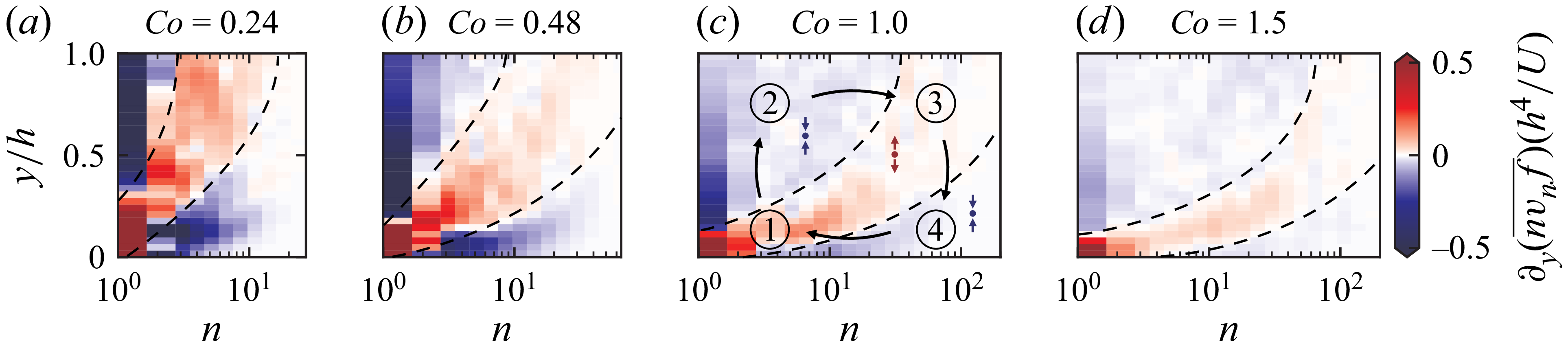
 ∂y(nvnf¯)
 (n,y)
 Co>0
 ∂y(nvnf¯)>0
 ∂y(nvnf¯)<0
 nvnf¯
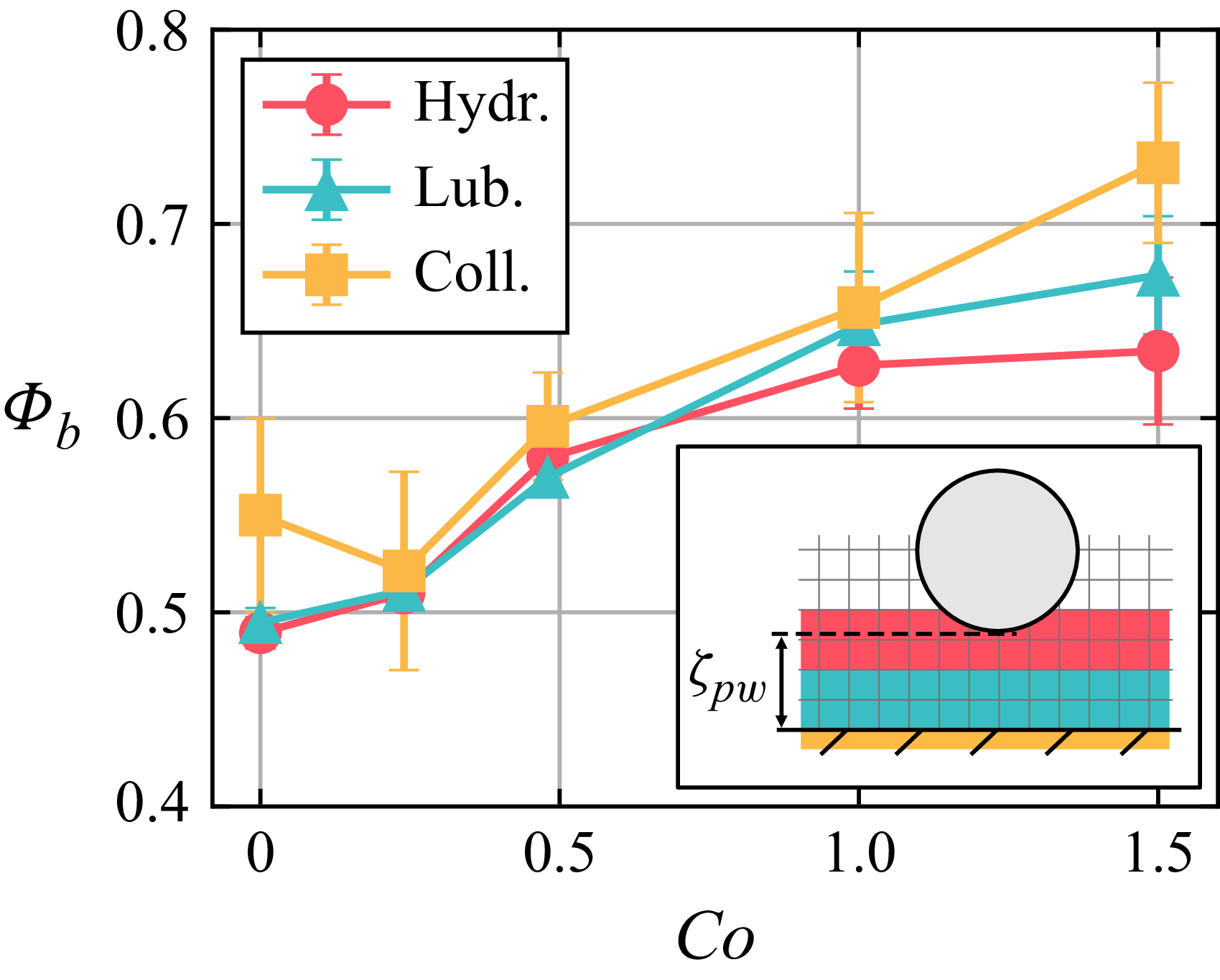
 Φb
 Co
 ζpw

 z
 n>2
 ϕ>10−3
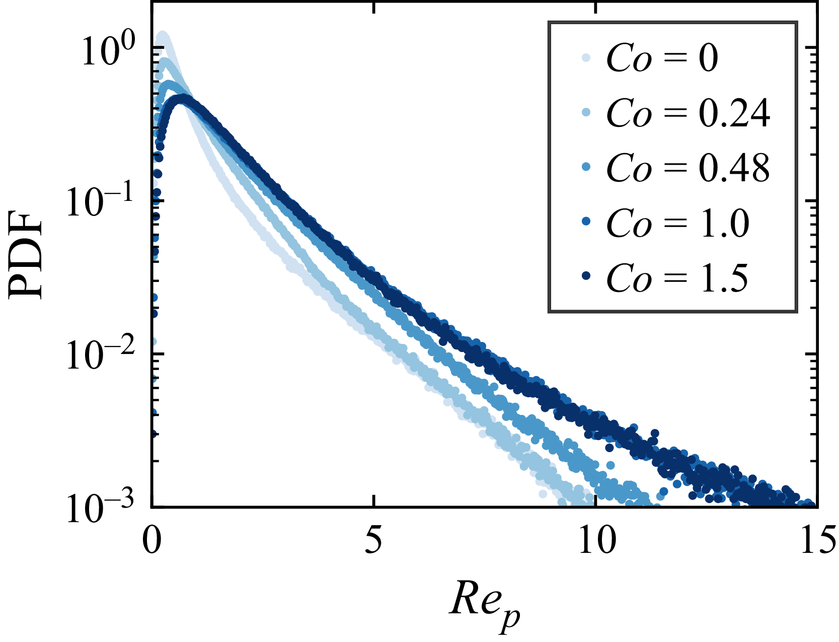
 Rep
 Teq
 Co
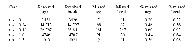
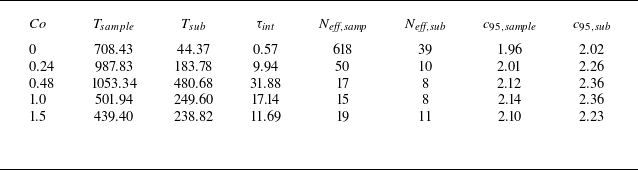
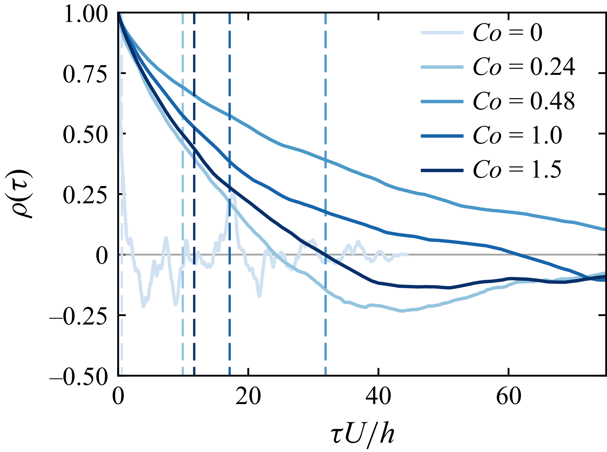
 Co
 τint

 Q¯
 Ta¯
 Tb¯
 ∂y(nvnf¯)
 n=1
 n∈{2,3}
 3
 Co>0
 y/h∈[0,1]
 y=d
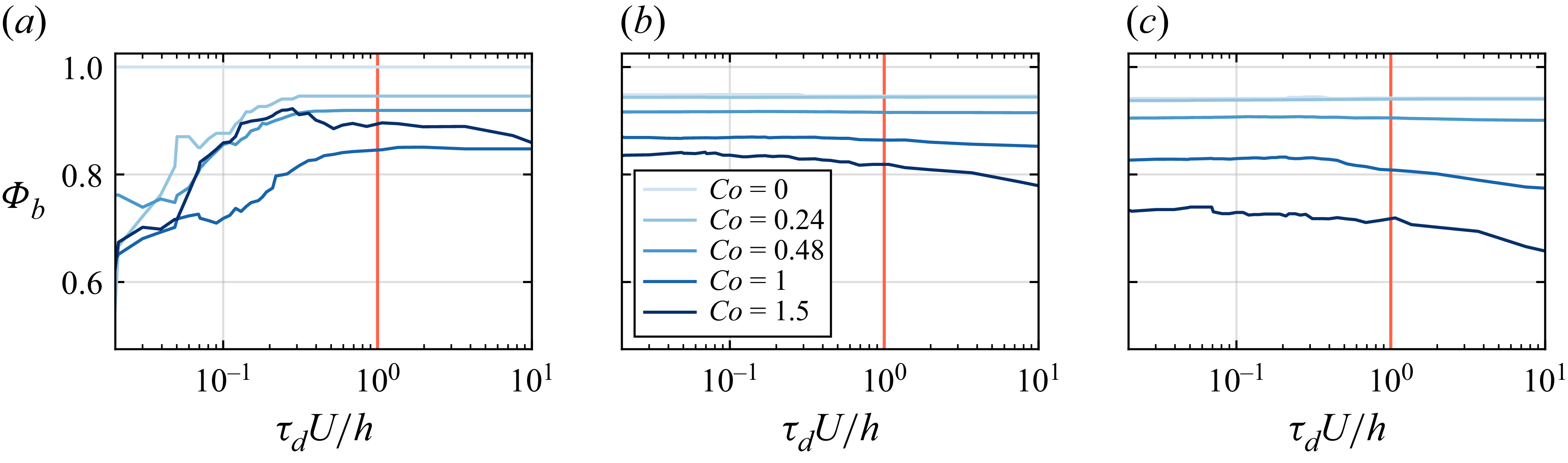
 Φb
 τd
 τd=h/U


 Open access

