





1. Introduction
In recent years, deep reinforcement learning (DRL) has emerged as a promising data-driven technique for handling the chaotic dynamics of fluid flow systems. Deep reinforcement learning has shown potential across a wide range of applications in fluid mechanics, including autonomous navigation (Tonti et al. Reference Tonti, Rabault and Vinuesa2025; Xiong et al. Reference Xiong, Liu, Wang, Ong and Zhu2025), wall-modelled large-eddy simulations (Bae & Koumoutsakos Reference Bae and Koumoutsakos2022; Zhou & Bae Reference Zhou and Bae2024), subgrid-scale modelling (Novati et al. Reference Novati, de Laroussilhe and Koumoutsakos2021; Kurz et al. Reference Kurz, Offenhäuser and Beck2023), Reynolds-averaged Navier–Stokes modelling (Fuchs et al. Reference Fuchs, von Saldern, Kaiser and Oberleithner2024), flow control (Verma et al. Reference Verma, Novati and Koumoutsakos2018; Guastoni et al. Reference Guastoni, Rabault, Schlatter, Azizpour and Vinuesa2023) and shape optimisation (Li et al. Reference Li, Zhang and Chen2021; Viquerat et al. Reference Viquerat, Rabault, Kuhnle, Ghraieb, Larcher and Hachem2021).
Owing to its intrinsic decision-making capabilities, DRL is particularly well suited for control problems, especially for active flow-control (AFC) applications. Deep reinforcement learning can discover and apply effective closed-loop control laws in dynamically evolving environments, learning sophisticated strategies that often outperform traditional methods relying on fixed actuation frequencies or predefined laws (Rodriguez et al. Reference Rodriguez, Lehmkuhl and Borrell2020; Sun et al. Reference Sun, Bahri, Jabbal, Stryczniewicz, Jefferson-Loveday, Stefes and Büscher2025). Therefore, DRL-AFC systems offer a promising approach for safer and more sustainable transport technologies.
In § 1.1, we first review the traditional AFC methods commonly applied to wings. Section 1.2 then outlines the DRL-based AFC studies present in the literature. Section 1.3 examines the complexities of the baseline problem considered in this study. Finally, the contributions of the present work are summarised in § 1.4.
1.1. Active flow control in wings
Among AFC techniques, steady uniform suction and blowing, as well as periodic suction and blowing, have been widely employed. In these control strategies, the actuation intensity is often characterised by the momentum coefficient
 $C_\mu = (\rho S_{\textit{jet}} U^2_{\textit{jet}})/(\rho S_{\textit{ref}} U^2_\infty )$
; where
 $\rho$
is the fluid density,
 $S_{\textit{jet}}$
the jet control surface,
 $S_{\textit{ref}}$
the characteristic reference area,
 $U_{\textit{jet}}$
the jet velocity and
 $U_\infty$
the free-stream velocity. Here, the reference area is taken as the airfoil chord
 $c$
times the corresponding span width
 $L_z$
.
In steady suction, low-momentum fluid is removed from the boundary layer while higher-momentum fluid is drawn toward the wall, thereby delaying flow separation and promoting flow attachment. Zhang et al. (Reference Zhang, Zhang, Chen and Tang2017) found that optimal control is achieved when the suction region is located just downstream of the separation point. Zhi-yong et al. (Reference Zhi-yong, Wang-long, Zhi-hua, Xiao-hui and Chen-chao2018) demonstrated that suction momentum has a more significant influence on aerodynamic performance than the suction angle. Both studies found that minimum drag and maximum aerodynamic efficiency occur at intermediate values of the momentum coefficient.
Conversely, steady uniform blowing injects momentum into the boundary layer, re-energising the flow and enhancing its ability to overcome adverse pressure gradients. This approach is commonly used in circulation control applications (Chen et al. Reference Chen, Seele and Wygnanski2012; Radespiel et al. Reference Radespiel, Burnazzi, Casper and Scholz2016). Blowing has also been shown to reduce skin-friction drag in turbulent boundary layers when low-intensity wall-normal injection is applied (Kametani & Fukagata Reference Kametani and Fukagata2011; O’Connor et al. Reference O’Connor, Diessner, Wilson, Whalley, Wynn and Laizer2023). However, this can also lead to increased pressure drag in the presence of adverse pressure gradients, potentially resulting in higher overall drag in aerodynamic configurations such as wings (Atzori et al. Reference Atzori, Vinuesa, Fahland, Stroh, Gatti, Frohnapfel and Schlatter2020).
The periodic combination of suction and blowing with zero mean mass flux over a complete actuation cycle is widely used for separation control and stall delay. Typically referred to as synthetic jets or zero-net-mass-flux (ZNMF) actuation (Glezer & Amitay Reference Glezer and Amitay2002), this approach exploits natural flow instabilities by utilising nonlinear resonance and frequency lock-in to reorganise the disordered and chaotic flow into concentrated lifting vortices (Wu et al. Reference Wu, Lu, Denny, Fan and Wu1998). Therefore, unlike steady methods, their effectiveness relies not only on momentum intensity but also on the unsteady generation of vortical structures that enhance mixing and momentum transfer. Consequently, synthetic jets can achieve comparable lift enhancements with substantially lower momentum input than steady actuation (Seifert et al. Reference Seifert, Darabi and Wyganski1996).
The effectiveness of ZNMF actuation is then primarily governed by the non-dimensional forcing frequency
 $F^{+}=fc/U_\infty$
, in addition to the momentum coefficient. Previous studies have consistently shown that forcing at
 $F^+ \approx 1$
, corresponding to the order of the natural wake shedding frequency, is the most effective for large-scale separation control (Gilarranz et al. Reference Gilarranz, Traub and Rediniotis2005; You & Moin Reference You and Moin2008; Raju et al. Reference Raju, Mittal and Cattafesta2008; Buchmann et al. Reference Buchmann, Atkinson and Soria2013; Zhang & Samtaney Reference Zhang and Samtaney2015).
For such excitation frequencies, optimal performance is typically achieved within a moderate range of momentum coefficients, with reported values around
 $0.01\lt C_\mu \lt 0.015$
(McCormick Reference McCormick2000; Rodriguez et al. Reference Rodriguez, Lehmkuhl and Borrell2020). Furthermore, the required momentum coefficient decreases when the forcing location is placed close to the separation point (Amitay et al. Reference Amitay, Smith, Kibens, Parekh and Glezer2001; Feero et al. Reference Feero, Lavoie and Sullivan2017).
1.2. Deep reinforcement learning for active flow control
Since the early work of Rabault et al. (Reference Rabault, Kuchta, Jensen, Réglade and Cerardi2019) on the stabilisation of a two-dimensional (2-D) cylinder wake at a Reynolds number of
 $ \textit{Re}_D = 100$
, DRL has evolved from controlling low-
 $ \textit{Re}$
laminar flows (Tang et al. Reference Tang, Rabault, Kuhnle, Wang and Wang2020; Varela et al. Reference Varela, Suárez, Alcántara-Ávila, Miró, Rabault, Font, García-Cuevas, Lehmkuhl and Vinuesa2022) to managing weakly turbulent regimes (Ren et al. Reference Ren, Rabault and Tang2021; Varela et al. Reference Varela, Suárez, Alcántara-Ávila, Miró, Rabault, Font, García-Cuevas, Lehmkuhl and Vinuesa2022) up to
 $ \textit{Re}_D = 2000$
; where
 $ \textit{Re}_D = \rho U_\infty D/\mu$
is defined using the cylinder diameter
 $D$
as the characteristic length and
 $\mu$
denotes the fluid viscosity. These early studies demonstrated that DRL agents can outperform periodic forcing by identifying non-trivial control strategies that suppress vortex shedding in 2-D cylinders with greater energy efficiency.
More recently, the extension to three-dimensional (3-D) and fully turbulent flows has been enabled by two key developments: (i) multi-environment parallelisation, where multiple computational fluid dynamics (CFD) simulations are run concurrently to accelerate the training (Rabault & Kuhnle Reference Rabault and Kuhnle2019); and (ii) multi-agent reinforcement learning (MARL), which overcomes the ‘curse of dimensionality’ arising when controlling multiple actuators simultaneously (Belus et al. Reference Belus, Rabault, Viquerat, Che, Hachem and Reglade2019). This framework has facilitated drag reduction in turbulent channel flows at around
 $ \textit{Re}_\tau = 180$
(Guastoni et al. Reference Guastoni, Rabault, Schlatter, Azizpour and Vinuesa2023; Sonoda et al. Reference Sonoda, Liu, Itoh and Hasegawa2023) and the control of 3-D cylinder wakes up to
 $ \textit{Re}_D = 3900$
(Suárez et al. Reference Suárez, Alcántara-Ávila, Miró, Rabault, Font, Lehmkuhl and Vinuesa2025a
,Reference Suárez, Alcántara-Ávila, Rabault, Miró, Font, Lehmkuhl and Vinuesa
b
). Here, the friction Reynolds number is defined as
 $ \textit{Re}_\tau =\rho \, u_\tau \, \delta / \mu$
; with
 $u_\tau =\sqrt {\tau _w/\rho }$
the friction velocity,
 $\tau _w$
the wall shear stress and
 $\delta$
the boundary layer thickness. Furthermore, strategies like coarse-mesh training (Font et al. Reference Font, Alcántara-Ávila, Rabault, Vinuesa and Lehmkuhl2025) and transfer learning from two to three dimensions (Chatzimanolakis et al. Reference Chatzimanolakis, Weber and Koumoutsakos2024; Liu et al. Reference Liu, Trujillo-Corona, Shu and Gross2025) have significantly mitigated the high computational cost of 3-D DRL-AFC.
A critical challenge for practical AFC is achieving high performance with minimal sensor data. Paris et al. (Reference Paris, Beneddine and Dandois2021) demonstrated that sensor placement can be optimised by selecting only the most informative observations for a 2-D cylinder. Similarly, Wang et al. (Reference Wang, Yan, Hu, Chen, Rabault and Noack2024) proposed a dynamic feature space lifting to achieve effective control with a single surface-mounted sensor. This is an important step towards practical DRL applications, which will necessarily rely on limited wall-based sensor input data. In related work, Yan et al. (Reference Yan, Li, Hu, Chen, Zhong and Noack2023) investigated wake control behind a square cylinder using surface pressure sensors.
Some authors have also investigated the use of alternative deep-learning architectures. While all of the aforementioned studies employed relatively simple multilayer perceptron (MLP) architectures, Jeon et al. (Reference Jeon, Rabault, Vasanth, Alcántara-Ávila, Baral and Vinuesa2025) demonstrated that using either group convolutional neural networks or positional encoding leads to faster and better learning. Following a similar approach, Kurz et al. (Reference Kurz, Kaushik, Blind, Kopper, Schwarz, Rodach and Beck2025) examined the benefits of graph neural networks (GNN). Although both MLP and GNN achieved similar average drag reductions, the GNN showed improved generalisation due to their inherent invariance to input ordering. Other researchers have focused on enhancing the controller’s perception and interpretability. Cavallazzi et al. (Reference Cavallazzi, Guastoni, Vinuesa and Pinelli2025) employed a convolutional neural network for feature extraction before passing the state to the agent, and Beneitez et al. (Reference Beneitez, Cremades, Guastoni and Vinuesa2025) integrated explainable deep learning for targeting specific turbulence-sustaining structures in an open channel, leading to more physically consistent control strategies. Separately, Weissenbacher et al. (Reference Weissenbacher, Borovykh and Rigas2025) examined transformer models, leveraging attention mechanisms to address partial observability with sparse sensing.
In the context of airfoils and wings, the combination of DRL with AFC remains limited, with most studies focusing on 2-D geometries at low Reynolds numbers. At
 $ \textit{Re}_c=3000$
(based on the airfoil chord
 $c$
), Wang et al. (Reference Wang, Mei, Aubry, Chen, Wu and Wu2022) and Garcia et al. (Reference Garcia, Miró, Suárez, Alcántara-Ávila, Rabault, Font, Lehmkuhl and Vinuesa2025) reported substantial aerodynamic performance improvements using DRL on a 2-D airfoil, outperforming periodic control in both effectiveness and energy efficiency. More recently, Liu et al. (Reference Liu, Trujillo-Corona, Shu and Gross2025) demonstrated that a DRL policy trained on 2-D flow around an airfoil at
 $ \textit{Re}_c=20\,000$
can be successfully transferred to the 3-D wing. In their study, the agent controlled the amplitude of a prescribed spanwise sinusoidal jet velocity profile. Other wing-related studies have also primarily focused on optimising static actuation parameters, such as actuator placement (Paris et al. Reference Paris, Beneddine and Dandois2023), rather than learning temporal control laws.
1.3. Flow past the NACA0012 wing at
 $ \textit{Re}_c=1000$

The flow past the NACA0012 airfoil at a Reynolds number of
 $ \textit{Re}_c=1000$
and angle of attack
 $\text{AoA}=20^\circ$
is studied. At this Reynolds number, the wake topology and flow dynamics undergo significant evolution as the angle of attack increases. Numerical and experimental investigations by Kurtulus (Reference Kurtulus2015) and Gupta et al. (Reference Gupta, Zhao, Sharma, Agrawal, Hourigan and Thompson2023) identified a primary transition at
 $\text{AoA} \gt 8^\circ$
, where the continuous vortex sheet in the wake evolves into an alternating vortex-shedding mode, resembling a von Kármán vortex street. This transition introduces periodic oscillations in the aerodynamic coefficients, a phenomenon further confirmed by Kouser et al. (Reference Kouser, Xiong, Yang and Peng2021).
As the angle of attack exceeds
 $\text{AoA} \gt 13^\circ$
, 3-D flow structures begin to develop, resulting in loss of the spanwise homogeneity of the vortex-shedding structures and the formation of parallel vortex rows with a characteristic spanwise wavelength. While 2-D simulations capture the initial shedding frequency, they fail to account for the spanwise instabilities that emerge in this regime (Kurtulus Reference Kurtulus2015; Kouser et al. Reference Kouser, Xiong, Yang and Peng2021). According to Kokash & Agbaglah (Reference Kokash and Agbaglah2024), this transition is attributed to the strong shear stress on the airfoil upper surface, which amplifies surface disturbances that evolve into characteristic streamwise rib-like vortices known as mode B (Williamson Reference Williamson1988). For configurations near
 $\text{AoA}=16^\circ$
, the resulting spanwise velocity exhibits a sinusoidal pattern with a characteristic wavelength between
 $\lambda _z/c=0.6$
(Kokash & Agbaglah Reference Kokash and Agbaglah2024) and
 $0.66$
(Kouser et al. Reference Kouser, Xiong, Yang and Peng2021). These values align closely with the mode B wavelengths reported by Barkley & Henderson (Reference Barkley and Henderson1996) for circular cylinders at an equivalent effective Reynolds number (
 $ \textit{Re}_D = Re_c \, \sin \text{AoA} \approx 280$
).
Finally, Kouser et al. (Reference Kouser, Xiong, Yang and Peng2021) demonstrated that the wake remains relatively stable in the range of
 $\text{AoA} = 14^\circ{-} 17^\circ$
, but progressively transitions to a chaotic and unstable wake as the angle of attack increases beyond
 $\text{AoA} \gt 18^\circ$
. This transition leads to the breakdown of the ordered pattern of spanwise-aligned vortex rows, reflecting the onset of a complex 3-D dynamics. For the 2-D case at
 $\text{AoA} = 20^\circ$
, Hoarau et al. (Reference Hoarau, Braza, Ventikos, Faghani and Tzabiras2003) identified that the aperiodicity of the von Kármán mode at higher angles of attack is lost via a period-doubling scenario. Moreover, they also studied the history of the 3-D transition mechanisms. In particular, they showed that the amplification of longitudinal and vertical vorticity components perturbs the rectilinear von Kármán rows, causing them to undulate into large-scale 3-D structures. Therefore, at
 $\text{AoA} = 20^\circ$
, the present case lies within this regime, where increased three-dimensionality and weakly turbulent behaviour make the flow particularly challenging for DRL.
1.4. Contribution
The present AFC-DRL framework, initially tested on a separated turbulent boundary layer at
 $ \textit{Re}_\tau = 750$
(Font et al. Reference Font, Alcántara-Ávila, Rabault, Vinuesa and Lehmkuhl2025) and further validated with a 3-D cylinder at
 $ \textit{Re}_D = 100$
(Montalà et al. Reference Montalà, Font, Suárez, Rabault, Lehmkuhl, Vinuesa and Rodriguez2024), advances the application of DRL to AFC in realistic aerodynamic configurations.
In contrast to previous studies (see table 1), the present work performs training directly in a fully 3-D flow configuration at a relatively high Reynolds number within the context of DRL, where sample inefficiency remains one of the major limitations. As a result, most existing studies are restricted to low Reynolds number regimes, while those addressing higher Reynolds numbers typically rely on simplified approaches, such as 2-D configurations (Wang et al. Reference Wang, Mei, Aubry, Chen, Wu and Wu2022; Garcia et al. Reference Garcia, Miró, Suárez, Alcántara-Ávila, Rabault, Font, Lehmkuhl and Vinuesa2025), transfer learning from reduced environments (Chatzimanolakis et al. Reference Chatzimanolakis, Weber and Koumoutsakos2024; Liu et al. Reference Liu, Trujillo-Corona, Shu and Gross2025) or simplified geometries (Suárez et al. Reference Suárez, Alcántara-Ávila, Miró, Rabault, Font, Lehmkuhl and Vinuesa2025a ; Font et al. Reference Font, Alcántara-Ávila, Rabault, Vinuesa and Lehmkuhl2025). By leveraging a solver accelerated through graphics processing units (GPUs), the present work overcomes part of this limitation and enables training in a fully 3-D setting. This allows the agent to interact with the inherently 3-D and chaotic dynamics characteristic of realistic turbulent flows. To the best of the authors’ knowledge, this represents the first application of DRL to control a 3-D wing CFD simulation.
A summary of the existing computational studies on DRL and its applications in AFC.

Table 1. Long description
A table comparing various studies on DRL applications in AFC. The table has four columns: References, Case study, Flow regime, and Algorithm. It contains 25 rows, each representing a different study. The References column lists the authors and year of each study. The Case study column describes the specific case studied, such as 2-D cylinder, 2-D wing, channel flow, and 3-D Rayleigh-Bénard. The Flow regime column provides the Reynolds number (Re_D or Re_t) or Rayleigh number (Ra) for each study. The Algorithm column lists the algorithms used, such as PPO, SAC, DDPG, and V-Racer. Each row provides detailed information about the study, including the specific case, flow regime, and algorithm used.
Furthermore, the study aims to highlight the flexibility of DRL as an adaptive control framework. By varying the relative weighting of the reward function terms, the controller can prioritise different objectives, such as lift enhancement or drag reduction. Unlike classical periodic forcing, which is inherently fixed, the learned controller adjusts its actuation in response to instantaneous flow conditions and varying optimisation goals, pointing toward multi-objective and time-dependent flow control in realistic operating environments characterised by unsteady and uncertain conditions.
2. Methodology
In this work, numerical simulations are performed to investigate the flow past a 3-D NACA0012 wing section at a Reynolds number of
 $ \textit{Re}_c=1000$
and an angle of attack of
 $\text{AoA} =20^\circ$
, with spanwise-periodic boundary conditions. Additionally, the interaction of jets located along the wing surface is included in the simulations, with their mass-flow rates optimised through DRL.
Schematic of the DRL framework showing the MARL strategy.

The DRL-CFD framework is illustrated in figure 1. It consists of two main components: the CFD environment and the DRL agent. At the core of the agent lies a neural network (NN) that is responsible for mapping flow states to corresponding control actions. In the present work, the NN processes pressure data collected from sensors located within the flow domain (state) and determines the appropriate jet velocity to be applied back into the system (action). To refine its control policy, learning is achieved through an iterative process between the agent and the environment driven by trial and error. Therefore, the CFD solver and the agent exchange not only states and actions but also rewards. The reward function quantifies the effectiveness of a control action, typically incorporating aerodynamic performance metrics such as lift enhancement or drag reduction.
The environment is implemented using the SOD2D solver (Gasparino et al. Reference Gasparino, Spiga and Lehmkuhl2024), developed in Fortran 90 language, whereas the DRL agent is built using the TF-Agents library (Guadarrama et al. Reference Guadarrama2018) in Python. To overcome the ‘two-language’ set-up, both components are coupled via a Redis in-memory database managed through the SmartSim API (Partee et al. Reference Partee, Ellis, Rigazzi, Shao, Bachman, Marques and Robbins2022). This enables efficient and low-overhead data exchange between the Fortran-based CFD solver and the Python-based DRL agent. The resulting framework is called SmartSOD2D (Font et al. Reference Font, Alcántara-Ávila, Rabault, Vinuesa and Lehmkuhl2025) and was originally created as a fork of the RELEXI project (Kurz et al. Reference Kurz, Offenhäuser, Viola, Resch and Beck2022).
Further details for each component are provided in the following sections: § 2.1 describes the numerical set-up of the CFD simulations, while § 2.2 explains the DRL configuration.
2.1. Computational fluid dynamics configuration
To predict the dynamic evolution of the system, the incompressible Navier–Stokes equations are integrated numerically. These equations are written as
 \begin{align} \frac {\partial u_i}{\partial x_{i}} = 0 , \\[-28pt] \nonumber \end{align}
 \begin{align} \frac {\partial u_i}{\partial t} + \frac {\partial }{\partial x_{\kern-1pt j}}(u_{i} u_{j}) - \frac {\mu }{\rho } \frac {\partial ^2 u_{i}}{\partial {x_{\kern-1pt j}} \partial {x_{\kern-1pt j}}} + \frac {1}{\rho } \frac {\partial p}{\partial x_{i}} = 0 , \\[0pt] \nonumber \end{align}
where
 $u_i=(u,v,w)$
and
 $p$
denote the velocity and pressure fields, respectively.
To solve these equations, the SOD2D solver is used (Gasparino et al. Reference Gasparino, Spiga and Lehmkuhl2024). This is a GPU-enabled spectral-element method (SEM; Patera Reference Patera1984) code developed at the Barcelona Supercomputing Center (BSC). The flow solver employs projection stabilisation to prevent numerical oscillations arising from dominant convection while introducing minimal numerical dissipation. Aliasing effects caused by the reduced-order integration of convective terms in the SEM are mitigated using a skew-symmetric splitting approach (Kennedy & Gruber Reference Kennedy and Gruber2008). Temporal discretisation is performed with a third-order Backward Differentiation Formula with third-order explicit extrapolation operator-splitting scheme to solve the velocity–pressure coupling, enabling equal-order interpolation of both velocity and pressure (Karniadakis et al. Reference Karniadakis, Israeli and Orszag1991). This solver is designed for high-fidelity simulations, and its scalability and computational efficiency on distributed accelerator-based architectures make it well suited for DRL applications, where rapid CFD data generation is crucial for the training.
The computational domain extends over
 $L_x/c = [-15,16]$
,
 $L_y/c = [-15,15]$
and
 $L_z/c = [0,3]$
in the streamwise, cross-stream and spanwise directions, respectively, with the wing leading edge located at the origin, i.e.
 $(x,y)/c = (0.0, 0.0)$
. A 2-D slice of the mesh in the
 $x{-}y$
plane is illustrated in figure 2. An unstructured hexahedral mesh is employed throughout the domain, with a more regular and wall-aligned element arrangement in the vicinity of the wing. Since a SEM is used, each element shown in the figure contains several integration points distributed according to the Gauss–Lobatto quadrature. In this work, fourth-order polynomial functions are employed (
 $p=4$
). The 2-D mesh contains around
 $N_{xy} = 1.05 \times 10^5$
degrees of freedom (DoF). This mesh is then extruded along the spanwise (or
 $z$
) direction with a total of eighteen spectral elements, corresponding to
 $N_z = 73$
integration points. This yields a 3-D mesh containing approximately
 $N_{xyz} =7.6 \times 10^6$
DoF. To determine the appropriate mesh resolution, a mesh sensitivity analysis is presented in Appendix A.
Visualisation of the computational mesh. The full domain is shown on the left, while a zoomed-in view around the wing is displayed on the right. Only the spectral elements are shown, whereas Gauss–Lobatto integration points are not displayed. The red dot indicates the origin of the coordinate system, while the green triangles denote the locations of the jets.

At the inlet, a constant free-stream velocity
 $U_\infty$
is imposed, corresponding to the target Reynolds number. This velocity is decomposed into the
 $x$
and
 $y$
directions according to the defined angle of attack. At the outlet, zero-gradient conditions with constant pressure are applied. The no-slip boundary condition is enforced on the wing surface, while periodic boundary conditions are imposed in the spanwise direction. Finally, on the jet surfaces, Dirichlet boundary conditions are used to specify the target jet velocity when AFC is active. This velocity is uniform across the entire jet outlet and oriented towards the
 $y$
-axis of the global coordinate system.
To explore 3-D actuations without causing excessive computational cost during DRL training, a MARL strategy is adopted (Belus et al. Reference Belus, Rabault, Viquerat, Che, Hachem and Reglade2019). Leveraging the spanwise invariance of the flow, the computational domain is partitioned into several subdomains referred to as MARL pseudo-environments, each featuring an independent jet actuator spanning the entire width of the subdomain. A single, shared policy is used for all the MARL pseudo-environments at the same time, which processes local state information to output a different individual jet velocity to each pseudo-environment. This set-up is schematised in figure 1 and has been successfully applied in related studies (Suárez et al. Reference Suárez, Alcántara-Ávila, Miró, Rabault, Font, Lehmkuhl and Vinuesa2025a , Reference Suárez, Alcántara-Ávila, Rabault, Miró, Font, Lehmkuhl and Vinuesab ; Font et al. Reference Font, Alcántara-Ávila, Rabault, Vinuesa and Lehmkuhl2025).
In this study, three MARL pseudo-environments are defined (
 $n_{\textit{MARL}} = 3$
). Within every subdomain, two jets are present: one near the leading edge of the wing at approximately
 $x/c = 0.01$
, and the other further downstream at
 $x/c = 0.4$
(as indicated in figure 2). Both jets span the entire width of their respective subdomains, i.e.
 $L_{z,\textit{jet}} = L_z/3 = 1.0c$
, and extend an arc length of
 $L_{xy, \textit{jet}}= 0.03c$
along the chord-wise direction. Thus, the corresponding individual jet surface can be calculated as
 $S_{\textit{jet}} = L_{z,\textit{jet}} \times L_{xy, \textit{jet}}$
. The agent directly controls the upstream jet, while the velocity of the downstream jet is set to have the opposite mass-flow rate, ensuring ZNMF jets and hence mass conservation at every time step. The agent is restricted to exploring values within the range
 $U_{\textit{jet}}/U_\infty = [-1.125, 1.125]$
.
For the state representation
 $s_t$
, each pseudo-environment uses pressure data from 90 sensors distributed across its mid-span plane. As shown in figure 3, the sensor layout is designed based on the flow structures observed in the uncontrolled case. The sensors are positioned above the wing, within the region where the wake is most prominent, aiming to capture both the main separation bubble and the downstream wake dynamics. Moreover, to account for 3-D flow characteristics, the DRL agent input combines the data from the 90 probes in its own MARL environment with those adjacent on either side, resulting in an input size of
 $90 \times 3 = 270$
probes.
Sensor locations used as the DRL agent state, superimposed on a snapshot of the baseline flow field: zoomed view shows instantaneous velocity magnitude, general 3-D view shows Q-criterion (the second invariant of the velocity gradient tensor) iso-contours
 $Q c^2/U^2_\infty=0.1$
coloured by velocity magnitude.

Finally, to further accelerate the data-collection process, ten independent CFD simulations are executed in parallel during training (
 $n_{\textit{CFD}} = 10$
), following the approach proposed by Rabault & Kuhnle (Reference Rabault and Kuhnle2019). As a result, each training episode yields
 $n_{\textit{MARL}} \times n_{\textit{CFD}} = 30$
distinct state–action–reward trajectories
 $\tau$
used to perform a single training step of the agent. The resulting speed-up achieved by employing
 $n_{\textit{en}v}=n_{\textit{MARL}} \times n_{\textit{CFD}}$
parallel environments is further analysed in Appendix B.
The total episode duration is set to
 $T_{\textit{eps}} = 10.52 U_\infty / c$
, corresponding to six vortex-shedding cycles of the baseline flow. Each pseudo-environment performs 120 discrete control actions per episode, resulting in an action duration of
 $T_{\textit{act}} = T_{\textit{eps}} / 120 = 0.088 U_\infty / c$
. This duration corresponds to roughly
 $5\,\%$
of the baseline vortex-shedding period, which has been found sufficient in the literature to provide control authority over the system (Rabault & Kuhnle Reference Rabault and Kuhnle2019).
In order to avoid spurious, non-physical oscillations in the numerical simulation, the newly predicted action is not applied directly to the environment. Instead, exponential smoothing is used to interpolate between successive discrete actions
 $a_{t-1} \rightarrow a_{t}$
, following the approach of Suárez et al. (Reference Suárez, Alcántara-Ávila, Miró, Rabault, Font, Lehmkuhl and Vinuesa2025a
,
Reference Suárez, Alcántara-Ávila, Rabault, Miró, Font, Lehmkuhl and Vinuesab
). As a result, the control signal evolves continuously within the CFD environment, reaching the target value
 $a_t$
at the end of the action period
 $T_{\textit{act}}$
, when a new action is provided by the agent.
At the end of each episode, the trajectories
 $\tau$
gathered across the ten parallel CFD simulations are combined into a batch, which the agent then uses to perform a training step. Once this is completed, simulations are re-launched to generate data for the next episode. Each simulation has an equal probability of restarting from either the baseline scenario or the final state of the preceding episode. This ensures that the DRL agent observes long-term controlled flow features while still effectively learning the highly dynamic initial transition phase from the uncontrolled to controlled regime. An overview of all parameters employed in the CFD environment is provided in table 2.
Summary of the CFD environment parameters utilised in this study.

Table 2. Long description
The table presents parameters and their values used in a CFD environment study. It has two columns: Parameter and Value. The table contains 12 rows with various parameters and their corresponding values. Row 1: Number of DoF (N xyz), 7.6 M. Row 2: Domain size ([ΔL x, ΔL y, ΔL z]), [31 c,"30 c", 3 c]. Row 3: Episode duration (T eps c / U ∞), 10.52. Row 4: Actions/episode, 120. Row 5: Parallel CFD environments (n CFD), 10. Row 6: MARL pseudo-environments (n MARL), 3. Row 7: Restart baseline/previous eps, 50/50 percent. Row 8: Jet surface (L xy,jet × L xy,jet), 1.0 c × 0.03 c. Row 9: Jet velocity range (U jet / U ∞), [-1.125, 1.125]. Row 10: Front jet location (x / c), 0.01. Row 11: Rear jet location (x / c), 0.4. Row 12: State size (variable), 90 × 3 (pressure).", "EDH": "
2.2. Agent configuration
The interaction between the agent and the environment is modelled as a Markov decision process. At each discrete time
 $t$
, the agent receives a state
 $s_t$
and selects an action
 $a_t$
according to a policy
 $\pi _\theta (a_t \mid s_t)$
. In DRL, a NN is used to approximate this policy. Following the execution of action
 $a_t$
the environment evolves from state
 $s_{t}$
to the next state
 $s_{t+1}$
according to the incompressible Navier-Stokes equations. It then returns a scalar reward
 $R_{t+1}$
, which quantifies the quality of the selected action
 $a_t$
.
This process continues sequentially until the end of the episode, resulting in a trajectory of the form
 $\tau = \{(s_0, a_0, R_1, s_1),\ (s_1, a_1, R_2, s_2),\ \ldots ,\ (s_{t}, a_{t}, R_{t+1}, s_{t+1})\}$
, which is then used to refine the policy during the training. In this work, a batch of trajectories collected from
 $n_{\textit{en}v}$
parallel environments is used to perform each training step. Each individual rollout generated by a single environment is referred to as a MARL episode. The objective throughout this learning process is to maximise the expected return, defined as the cumulative discounted reward
 \begin{align} G_t = R_{t+1} + \gamma R_{t+2} + \gamma ^2 R_{t+3} \ldots = \sum _{l=0}^{\infty } \gamma ^{l} R_{t+1+l}, \end{align}
where
 $\gamma \in [0, 1)$
is the discount factor that balances the importance of immediate versus future rewards. For the present computations, the discount factor is set to
 $\gamma = 0.99$
.
The proximal policy optimisation (PPO) algorithm is employed to iteratively improve the agent’s policy over the course of training (Schulman et al. Reference Schulman, Wolski, Dhariwal, Radford and Klimov2017). Proximal policy optimisation is a model-free, on-policy and actor-critic method, where the actor learns the policy
 $\pi _\theta (a_t | s_t)$
and the critic estimates the value function
 $V_\theta (s_t)$
, representing the expected return under the current policy. This is then used to compute the advantage function
 $A_t$
that guides the training of the actor.
Both the actor and critic networks consist of two separate MLPs, each featuring two hidden layers of 512 neurons. Training is performed using the Adam optimiser (Kingma & Ba Reference Kingma and Ba2014) with a learning rate of
 $\text{LR}=5 \times 10^{-4}$
. The critic is trained by minimising the mean squared error between the predicted and the observed returns, while the actor updates its policy parameters guided by the estimated advantages, which in this work are computed using the generalised advantage estimation (GAE; Schulman et al. Reference Schulman, Moritz, Levine, Jordan and Abbeel2015). This enables the actor to increase the likelihood of actions that yield higher-than-expected returns during training. Detailed mathematical formulations of the PPO agent are provided in Appendix C.
In this work, the training is conducted using the reward function
 $R_i$
written in (2.4), where the index
 $i$
denotes the corresponding MARL pseudo-environment. Thus, the reward accounts for both local
 $r_i$
and global performance, represented by the mean reward computed across all pseudo-environments, with the weighting factor
 $\eta \in [0, 1]$
modulating the relative importance of each term. In this study, this is set to
 $\eta = 0.8$
 \begin{align} R_i = \eta \; r_i + (1-\eta )/n_{\textit{MARL}} \sum _{j=1}^{n_{\textit{MARL}}}r_j , \\[-28pt] \nonumber \end{align}
 \begin{align} r_i = (C_{d,\textit{base}} - C_d) - \alpha \; | C_l - C_{l,\textit{avg}} | + \beta (C_l - C_{l,\textit{base}}) . \\[0pt] \nonumber \end{align}
The local reward
 $r_i$
is calculated as defined in (2.5). This comprises three contributions: The first term encourages a reduction in drag coefficient
 $C_d$
relative to the baseline
 $C_{d,\textit{base}}$
; the second penalises fluctuations in the lift coefficient, where
 $C_{l,\textit{avg}}$
corresponds to the accumulated mean lift coefficient over the course of the episode; and the third promotes an increase in lift coefficient
 $C_l$
compared with the baseline
 $C_{l,\textit{base}}$
.
The lift and drag coefficients are calculated as
 $C_l = l / (0.5 \rho U_\infty S_{\textit{ref}})$
and
 $C_d = d / (0.5 \rho U_\infty S_{\textit{ref}})$
, where
 $l$
and
 $d$
denote the aerodynamic force components in the cross-stream and streamwise directions relative to the free-stream velocity
 $U_\infty$
. These coefficients are averaged over the duration of each action period
 $T_{\textit{eps}}$
before computing the reward.
Two separate training runs are conducted to assess the sensitivity to the reward hyperparameters. In both cases,
 $\alpha =0.3$
, while
 $\beta$
is set to
 $0.0$
in the first training and
 $0.5$
in the second. These configurations are hereafter referred to as NLT-OFF and NLT-ON, corresponding to the net lift term being deactivated (
 $\beta = 0.0$
) and activated (
 $\beta = 0.5$
), respectively. All the hyperparameters used for training the PPO agent are listed in table 3.
Summary of PPO hyperparameters used during training.

Table 3. Long description
A table with two columns and twelve rows. The columns are labeled Parameter and Value. The table lists various hyperparameters used during training and their corresponding values. Row 1: Discount factor (gamma), 0.99. Row 2: GAE lambda (lambda), 0.95. Row 3: Value loss coefficient (c1), 0.5. Row 4: Entropy coefficient (c2), 0.0. Row 5: Clipping ratio (epsilon), 0.3. Row 6: Learning rate (LR), 5 times 10 to the power of -4. Row 7: MLPs architecture (neurons times layers), 512 times 2. Row 8: Reward local balance (eta), 0.8. Row 9: Lift-fluctuation penalty (alpha), 0.3. Row 10: Lift improvement bonus (beta), 0.0 and 0.5. Row 11: Optimiser type, Adam. Row 12: Epochs per optimisation, 30.
3. Results
3.1. Baseline validation
Before introducing AFC strategies, the uncontrolled scenario is validated to ensure the accuracy and reliability of the numerical set-up. This case serves as both a baseline for evaluating performance improvements achieved through DRL-based control and the initial condition upon which control inputs will be applied.
Variation of the mean (a) lift coefficient and (b) drag coefficient with the angle of attack, comparing the present results with the literature.

Figures 4(a) and 4(b) compare the mean lift and drag coefficients reported in the literature for different angles of attack. As can be observed, the discrepancies between the 2-D and 3-D simulations become increasingly pronounced as 3-D effects emerge beyond
 $\text{AoA} \gt 13^\circ$
, with differences growing larger at higher angles. Superimposed on these plots are the mean lift and drag coefficients obtained in this study, which closely match the 3-D results reported by Kouser et al. (Reference Kouser, Xiong, Yang and Peng2021) for the same angle of attack.
As discussed in § 1.3, the flow lies in a regime characterised by strong separation and chaotic three-dimensionalities in the wake. Previous studies report periodic spanwise wavelengths of
 $\lambda _z/c \approx 0.60 - 0.66$
at
 $\text{AoA}=16^\circ$
(Kouser et al. Reference Kouser, Xiong, Yang and Peng2021; Kokash & Agbaglah Reference Kokash and Agbaglah2024). Anticipating similar values at the current angle of attack, the chosen spanwise domain length of
 $L_z/c = 3.0$
is sufficient to capture this dynamics.
The statistical analysis of the baseline flow was performed over 40 vortex-shedding cycles after reaching the statistically steady state, corresponding to approximately
 $70 c/U_\infty$
. After this sampling period, the running averages of
 $C_l$
and
 $C_d$
, as well as their standard deviations, reached a plateau, indicating statistical convergence of the results. For more details, see Appendix A.
To quantitatively assess the present results, table 4 reports the statistics of the aerodynamic forces, together with the 2-D and 3-D results from Kouser et al. (Reference Kouser, Xiong, Yang and Peng2021). The table includes the mean lift coefficient, the standard deviation of the lift coefficient, the drag coefficient and the vortex-shedding Strouhal number
 $\textit{St}=f c/U_\infty$
, where
 $f$
denotes the frequency. Here,
 $f$
is obtained from the peak of the power-spectral density of the lift coefficient signal. Except for the lift coefficient fluctuations
 $C^{\prime }_{l, \textit{rms}}$
, which are not reported in previous studies, the differences with respect to the literature are minimal:
 $|\Delta C_l| = 2.2\,\%$
,
 $|\Delta C_d| = 1.2\,\%$
and
 $|\Delta \textit{St}| = 3.7\,\%$
. Hence, it can be concluded that these results show good agreement with other 3-D simulations and follow the expected trends reported in the literature, confirming the validity of the numerical set-up used in this study.
Summary of key aerodynamic coefficients for the baseline case and the DRL-controlled scenarios, including the mean lift and drag, the r.m.s. of the lift fluctuations and the Strouhal number associated with vortex shedding. The baseline case is compared with other simulations reported in the literature.

Table 4. Long description
The table presents a comparison of key aerodynamic coefficients for various simulation cases. It includes five rows and five columns. The columns are labeled as Case ID, C_l, C’_l,rms, C_d, and St. The rows are labeled with different simulation cases: Kouser et al. (2021) 2-D sim., Kouser et al. (2021) 3-D sim., Baseline, DRL NLT-OFF, and DRL NLT-ON. Each row lists the corresponding values for the mean lift coefficient (C_l), the root mean square of the lift fluctuations (C’_l,rms), the drag coefficient (C_d), and the Strouhal number (St). Notable trends include variations in the lift and drag coefficients and the Strouhal number across different cases, with specific percentage changes indicated for the DRL-controlled scenarios compared to the baseline.
3.2. Deep reinforcement learning control: training
In the present work, two different DRL trainings are considered by varying the weighting factors that modulate the contribution of each term in the local reward function (see (2.5)). In this section, the results obtained using NLT-OFF (
 $\alpha = 0.3$
,
 $\beta = 0.0$
) and NLT-ON (
 $\alpha = 0.3$
,
 $\beta = 0.5$
) are analysed, where the main difference lies in the greater importance given to the lift coefficient (
 $\beta \gt 0$
) in NLT-ON. The remaining parameters are kept constant.
Evolution of the mean (a) lift coefficient, (b) drag coefficient, (c) lift coefficient fluctuations and (d) local reward over the last
 $5U_\infty /c$
of each episode during training. In each plot, a moving average is applied to smooth signals, while the individual data points are shown in a lighter, more transparent colour. The dashed black lines in (a) and (b) represent the baseline average value from the non-actuated case.

Figure 5 shows the evolution of the key aerodynamic parameters for both DRL policies during training, namely the lift coefficient
 $C_l$
, drag coefficient
 $C_d$
and the root mean square (r.m.s.) of the lift coefficient fluctuations
 $C^\prime _{l,\textit{rms}}$
, along with the local reward
 $r$
, which reflects a weighted combination of the previous parameters. For each MARL episode, these values are averaged over the last
 $5U_\infty /c$
and appended sequentially to the plot. A moving average with a window size equal to the number of parallel environments
 $n_{\textit{en}v}$
is then applied to smooth the resulting signals.
Training is conducted until a certain level of convergence is observed. In this case, the reward increases over the course of the training and reaches a plateau at around 2010 MARL episodes. At this point, training is stopped for both cases. In the present investigations, each training step combines the trajectories from every 30 MARL episodes, corresponding to the
 $n_{\textit{en}v} = n_{\textit{MARL}} \times n_{\textit{CFD}}$
environments running in parallel, resulting in a total of 67 training steps over the course of the training.
Each training step required approximately 10 minutes of wall-clock time on ten nodes of MareNostrum V, with each node equipped with four NVIDIA H100 GPUs and two Intel Xeon processors (80 CPU cores in total), leading to a total wall-clock time of around 11 hours per training case. This corresponds to a total computational cost of
 $440$
GPU-hours. The reported time includes both experience collection, during which the agents interact with the multiple environments, and training time, when the NN parameters
 $\theta$
are updated. Notably, the NN optimisation step accounts for less than 0.1 % of the total computational time, highlighting the computational bottleneck of CFD environments.
From the values of
 $C_l$
,
 $C_d$
and
 $C^\prime _{l,\textit{rms}}$
shown in figure 5, it is evident that each training run adopts a completely different strategy. Under NLT-OFF, the lift coefficient remains relatively flat and slightly higher than the baseline. However, both the drag coefficient and the lift fluctuations exhibit a notable decreasing trend, significantly contributing to the increase in total reward. In contrast, for NLT-ON, the reward improvement is primarily driven by the lift coefficient, which increases substantially above the baseline as training progresses. Nevertheless, the drag coefficient remains close to the baseline and even performs slightly worse, while the reduction in lift fluctuations is less pronounced compared with NLT-OFF.
These results confirm that adding a term favouring lift enhancement effectively promotes its increase. However, the method appears highly sensitive to the weighting coefficients
 $\alpha$
and
 $\beta$
, as even a change in
 $\beta$
alone leads to markedly different optimisation strategies.
In principle, the weighting factor of
 $\beta = 0.5$
was selected to balance the lift and drag terms in the reward formulation of (2.5), given that
 $C_{l,\textit{base}}$
is approximately twice
 $C_{d,\textit{base}}$
. Therefore, compared with the NLT-OFF scenario, one would intuitively expect a balance between drag reduction and lift enhancement under NLT-ON reward. However, in practice, it is observed that the agent predominantly optimises lift, highlighting one of the challenges associated with DRL-based control: identifying optimal parameters in the reward function for a given objective.
In the training curves shown in figure 5, the baseline values of
 $C_l$
and
 $C_d$
are included as black dashed lines for comparison, whereas no baseline line is plotted for
 $C^\prime _{l,\textit{rms}}$
. While the averaged coefficients observed during training are generally representative of those expected during evaluation, the r.m.s. lift-fluctuation coefficient remains substantially higher than the baseline value of
 $C^\prime _{l,\textit{rms}}=0.085$
. This is an expected consequence of the agent’s exploration process, which artificially introduces variance into the
 $C_l$
signal, thereby inflating the r.m.s. fluctuations. In this context, the evolution of
 $C^\prime _{l,\textit{rms}}$
during training should be interpreted more as an indicator that the model is learning and adapting, rather than as a representation of the final expected magnitudes.
Additionally, due to the stochastic nature of the DRL algorithm and the additional variability introduced by GPU operations in the CFD solver, slight differences may arise between different training runs of the same model. However, as shown in Appendix D, the results obtained across different runs remain well bounded and fall within a reasonable confidence interval.
3.3. Deep reinforcement learning control: evaluation
After the training phase, where the agent samples actions to discover those that may further increase the accumulated return (exploration), the evaluation mode is applied. In this mode, the most likely action produced by the policy is selected for each observed state (exploitation).
Temporal signals of the (a) lift and (b) drag coefficients when the DRL control is activated during exploitation compared with the baseline signals. (c) Power-spectral densities (PSDs) of the lift coefficient signals.

In figures 6(a) and 6(b), the lift coefficient and drag coefficient signals are shown against the baseline results once the control is activated (
 $t U_\infty /c \gt 0$
). Initially, during approximately
 $t U_\infty /c \approx 15$
, the flow transitions from the baseline to a new regime. Following this brief transient, the flow reaches a new statistically steady state. The averaged results are then integrated over
 $50\, U_\infty / c$
, which has been shown to be sufficient for convergence (see Appendix A). The resulting aerodynamic coefficients are summarised in table 4.
The performance differences between the two learned policies can be clearly visualised in the lift and drag signals in figures 6(a) and 6(b). When NLT-OFF is used, the agent primarily focuses on wake stabilisation, as evidenced by the substantial reduction in flow fluctuations and a more regular and periodic pattern of the lift signal, which ultimately leads to drag reduction. Although the drag term numerically dominates the reward function due to its larger weighting factor, the lift-fluctuation term consistently decreases throughout training (figure 5
c). In contrast, the drag contribution plateaus early (figure 5
b). This behaviour indicates that the agent has identified the wake stabilisation as the main mechanism to increase the reward, with drag reduction emerging as a secondary effect of the continuous suppression of lift fluctuations. This mechanism resembles the results reported by Rabault et al. (Reference Rabault, Kuchta, Jensen, Réglade and Cerardi2019) for a 2-D cylinder case, and later observed in the 3-D case by Suárez et al. (Reference Suárez, Alcántara-Ávila, Rabault, Miró, Font, Lehmkuhl and Vinuesa2025b
), where equivalent reward functions were employed. As indicated in table 4, this policy achieves a mean drag reduction of
 $21.1\,\%$
and a
 $54.1\,\%$
decrease in lift fluctuations, while maintaining the mean lift close to the baseline value, with only a slight increase of approximately
 $3.0\,\%$
.
By contrast, the performance under NLT-ON is markedly different. Here, the agent primarily focuses on increasing the lift coefficient, but this comes with notable drawbacks. The fluctuations in aerodynamic forces are substantially larger than in the baseline, and the drag shows no reduction. With this policy, the mean lift increases by
 $42.3\,\%$
, while the lift fluctuations and drag increase by
 $65.9\,\%$
and
 $3.5\,\%$
, respectively, as summarised in table 4. These performance trends for both rewards were already anticipated during training, as indicated by the evolution of the reward signals.
In both the
 $C_l$
and
 $C_d$
time signals, periodic patterns remain clearly visible after DRL control is applied, similar to the baseline flow, where strong vortex shedding dominates the dynamics. This is further supported by the lift coefficient spectra shown in figure 6(c), where distinct spectral peaks are present, indicating that the main vortex-shedding frequency is still active. This analysis was performed after discarding the transient period in the DRL cases. The corresponding Strouhal numbers are reported in table 4. While NLT-ON does not show an important variation of the Strouhal number compared with the baseline, under NLT-OFF, this is increased by approximately 14 %.
Control actions for (a) DRL NLT-OFF and (b) DRL NLT-ON from the onset of control activation. Only the front jets are shown, with each MARL pseudo-environment represented by a distinct colour.

Zoomed view of the control actions from figure 7 in the statistically steady state for (a) DRL NLT-OFF and (b) DRL NLT-ON. Only the front jets are displayed, and each MARL pseudo-environment is represented by a distinct colour. The corresponding PSDs are shown on (b) and (d), respectively, with offsets applied across the MARL pseudo-environments for clarity.

The instantaneous control actions
 $U_{\textit{jet}}/U_\infty$
applied by the DRL are shown in figure 7 for the two policies. Only the actions of the front jet are displayed, with each colour corresponding to one MARL pseudo-environment, thereby illustrating the variation of the action along the spanwise direction as well. As described in § 2.1, the rear jet simultaneously applies the opposite mass-flow rate to ensure mass conservation.
As observed in these plots, the agent initially destabilises the baseline flow before reaching a new statistically steady state. This behaviour was also reflected in the
 $C_l$
and
 $C_d$
signals in figure 6. Once the statistically steady state is reached (
 $t U_\infty /c \gt 15)$
, it becomes evident that the control strategy strongly depends on the selected reward. A zoomed view of the jet actions in the stationary regime is provided in figures 8(a) and figure 8(c). Additionally, the corresponding PSDs for the NLT-OFF and NLT-ON actions after discarding the initial transient are presented in figures 8(b) and 8(d), respectively.
Under NLT-OFF, the control actions are consistently negative, indicating suction by the front jet and corresponding blowing by the rear jet. The signals have a mean offset of around
 $U_{\textit{jet}}/U_\infty = -0.72$
, with minor fluctuations around this value. This corresponds to a momentum coefficient of
 $C_\mu = 0.016$
, based on the r.m.s. of the jet velocity. A periodic pattern can be identified, with peaks and valleys located at approximately the same location, although some chaotic variability persists across different MARL pseudo-environments. In this case, two dominant frequencies are detected. One at
 $\textit{St}=0.64$
, corresponding to the natural vortex-shedding frequency of the flow, as confirmed by the lift coefficient spectra in figure 6(c), and a sub-harmonic at
 $\textit{St}=0.32$
.
This strategy resembles the suction mechanism observed in previous AFC studies, where stabilising the wake is achieved by applying suction at the leading edge. By drawing extra momentum into the boundary layer at this critical location, the flow better overcomes the high curvature near the leading edge, thereby delaying shear layer separation. As demonstrated in figure 9(b), this shifts the shear layer closer to the suction surface, physically limiting the entrainment and growth of the trailing-edge vortex. Consequently, the cross-stream extent of the wake structures is reduced, leading to a narrower wake with smaller vertical spacing between vortex cores and an increased shedding frequency. The observed vortex-shedding frequency in this case is therefore driven primarily by flow stabilisation rather than by the DRL controller.
Time-averaged velocity streamlines with the velocity magnitude shown in the background. Results are presented for the (a) baseline, (b) DRL NLT-OFF and (c) DRL NLT-ON scenarios. Crosses indicate the locations of the vortex cores, and triangles denote the flow separation point at the leading edge.

In contrast, NLT-ON results in much more correlated signals across environments. Here, the actions follow a more 2-D and synchronised control strategy, with overlapping periodic signals. This strategy involves both suction and blowing, as the signals exhibit negative and positive values, although the mean value remains negative at approximately
 $U_{\textit{jet}}/U_\infty =-0.17$
. The amplitude of fluctuations is clearly higher than in the NLT-OFF case, which explains the increased values of
 $C^\prime _{l, \textit{rms}}$
observed earlier for this scenario. In this case, the r.m.s. of the jet velocity is
 $U_{\textit{jet, rms}}/U_\infty =0.58$
, corresponding to a momentum coefficient of
 $C_\mu =0.011$
. Furthermore, a single dominant frequency emerges in the actions, closely matching the natural vortex-shedding frequency of the uncontrolled flow, i.e.
 $\textit{St}=0.57$
.
This behaviour resembles periodic forcing strategies employed in previous AFC studies to delay stall. A frequency lock-in occurs, with the DRL agent effectively exploiting resonance. As shown in figure 9(c), the trailing-edge vortex is suppressed, while a persistent vortex remains near the suction surface. As later confirmed in the dynamical analysis, this resonant excitation drives lift enhancement through maximisation of the lifting vortex, indicating that the frequency is actively targeted by the DRL agent.
The fact that the DRL agent explicitly targets well-established control mechanisms reported in the literature indicates that it can identify and exploit physically meaningful strategies despite its data-driven nature. Moreover, the resulting momentum coefficients are consistent with those reported in prior studies (see § 3.4), although they are slightly higher, likely due to increased viscous effects associated with the lower Reynolds numbers considered here.
Visualisation of vortical structures using Q-criterion iso-contours
 $Q c^2/U_\infty ^2=0.1$
coloured by velocity magnitude. (a) Baseline, (b) DRL-control under NLT-OFF and (c) DRL-control under NLT-ON. On the left, the top view; and on the right, the perspective view.

In figure 10, the vortical structures of the controlled scenarios in the statistically steady state are compared against the baseline case using the Q-criterion iso-contours. In the uncontrolled scenario (figure 10
a), the periodic pattern of the rib-like structures of mode B is broken, and no clear periodicity is observed along the
 $z$
-direction. The high angle of attack leads to a significant separation, creating a low-pressure region that induces the formation of a vortex near the trailing edge (leading vortex), which partially entrains fluid above the suction side of the wing. This vortex interacts with the shear layer originating at the leading edge, leading to the generation of a new vortex (paired vortex). This process is illustrated in figure 11(a), which shows the temporal evolution of the flow over a shedding cycle. This figure also presents the same analysis for the two controlled cases, with each snapshot corresponding to the instants indicated as black dashed lines in figure 8.
 $z$
-Vorticity contours
 $\omega _z c/U_\infty \in [-10, 10]$
in the
 $x$
–
 $y$
plane over a vortex-shedding cycle for the (a) baseline uncontrolled scenario and the DRL-controlled scenarios under (b) NLT-OFF and (c) NLT-ON. Frame numbers 1, 2 and 3 in (b) and (c) correspond to the times highlighted in figures 8(a) and 8(c), respectively.

Figure 11. Long description
A diagram showing vorticity contours over a vortex-shedding cycle for baseline and controlled scenarios. Panel A: Baseline. The diagram shows three stages of vortex formation and shedding. The leading vortex and paired vortex are labeled. Panel B: DRL NLT-OFF. The diagram shows three stages of vortex formation and shedding with the DRL control mechanism turned off. The leading vortex and paired vortex are labeled. Panel C: DRL NLT-ON. The diagram shows three stages of vortex formation and shedding with the DRL control mechanism turned on. The leading vortex and paired vortex are labeled.
Under NLT-OFF, the wake exhibits a more organised pattern of rib-like structures, with a well-defined periodicity along the invariant direction compared with the baseline, as observed in figure 10(b). This transition from a massive, separated wake to a more confined, organised structure explains the emergence of the regular periodic patterns in the lift signal and is analogous to reducing the angle of attack, where homogeneous von Kármán vortex rows are recovered, and chaotic features are no longer observed. In this scenario, the detached leading vortex forms further downstream of the trailing edge due to the deflection of the shear layer towards the wing wall (see figure 11(b), left). Consequently, the wake is elongated along the streamwise direction, and the paired vortices are less separated vertically, which explains the reduction of the vortex-shedding amplitude and its shift to higher frequencies (see figure 11(b), right). By partially mitigating the adverse effects of vortex shedding, this mechanism leads to a reduction in fluctuations and, ultimately, in drag.
For NLT-ON, the flow exhibits a nearly 2-D behaviour, with well-defined vortex tubes along the
 $z$
-direction, as observed in figure 10(c). This is consistent with the nearly 2-D control actions applied by the agent in figure 8(c). However, the mechanism of formation of these vortices differs from the NLT-OFF and baseline scenarios. Here, the paired vortex is primarily generated by the oscillatory behaviour of the jet actions rather than by the breakdown of the shear layer induced by the primary vortex. When the front jet blows, it lifts the shear layer at the leading edge, creating a small low-pressure region here (figure 11(c), left). As a result, the shear layer begins to roll up, forming a vortex that subsequently breaks down when the front jet reverses to suction and the rear jet to blowing (figure 11(c), centre). This vortex is then convected downstream with the mean flow, generating a counter-rotating vortex as it passes the trailing edge (figure 11(c), right). Therefore, by contrast to what was observed before, in this case, the leading-edge vortex acts as the precursor to the trailing-edge vortex. This shift in the vortex-shedding dynamics, actively enforced by the DRL controller, supports the presence of a resonance mechanism underlying the control strategy, with the controller artificially creating prominent lifting vortices.
3.4. Classic control
To further investigate the benefits of DRL control, different classical control actuations are applied to the same wing configuration. Again, two jets are located at the leading edge and mid-chord locations, as defined in § 2.1. In this study, however, a homogeneous jet velocity is prescribed along the spanwise direction. The fixed control law used for the front jet is defined as
 \begin{align} \frac {U_{\textit{jet}}}{U_\infty } = \frac {A}{U_\infty } \; \text{sin}\left (2\pi f\frac {U_\infty }{c} \; t \right ) + \frac {A_{\textit{DC}}}{U_\infty } \; , \end{align}
while, similar to the DRL scenario, the rear jet instantaneously applies the opposite mass-flow rate. In (3.1), three key parameters need to be specified: the actuation amplitude
 $A$
, the actuation frequency
 $f$
and the steady component of the signal
 $A_{\textit{DC}}$
. To enable a comparison with the AFC strategy learned by the DRL agents, a range of parameters will be tested, following a traditional parametric study approach. The target frequencies are selected based on the vortex-shedding frequency of the uncontrolled scenario
 $\textit{St}_0$
, exploring values around this baseline, specifically
 $f U_\infty / c = [0.8, 1.0, 1.2]\;\textit{St}_0$
. For the actuation amplitude
 $A$
and the steady component
 $A_{\textit{DC}}$
, values are chosen relative to the maximum jet velocity explored by the DRL agents, i.e.
 $(U_{\textit{jet}}/U_\infty )_{\textit{max}} = 1.125$
. Specifically, the amplitude
 $A$
is tested at 100 %, 50 % and 25 % of this maximum, while the steady component
 $A_{\textit{DC}}$
is tested at −50 %, 0 % and 50 %.
Moreover, classical AFC actuations derived from the DRL solutions are also investigated. Specifically, the statistical characteristics of the DRL jet signals shown in figure 8, namely the dominant frequency (
 $f$
), mean jet velocity (
 $A_{\textit{DC}}$
) and standard deviation, are used to define an actuation following (3.1). More precisely, since a sinusoidal law is employed, the amplitude (
 $A$
) is selected such that the standard deviation of the resulting signal matches that of the DRL jet signal. The same two-jet configuration described previously is used. In addition, a simplified actuation case considering only the front leading-edge (LE) jet is also examined.
The statistics from all these simulations are collected over
 $50U_\infty /c$
convective time units after the initial transient, as was done previously for the DRL-controlled scenarios, which is sufficient for statistical convergence. Figure 12(a) presents the
 $C_l$
and
 $C_d$
coefficients obtained for all classic control cases, compared with the results from the DRL strategies and the uncontrolled baseline case, while figure 12(b) further illustrates the
 $C^\prime _{l, \textit{rms}}$
. The obtained results are quantitatively reported in Appendix E.
Results of the classic control parametric study compared against the uncontrolled baseline scenario (black ‘
 $+$
’ markers), the DRL-controlled cases under NLT-OFF (red ‘
 $+$
’ markers) and NLT-ON (orange ‘
 $+$
’ markers) and the classic controls derived from the corresponding DRL cases (red and orange ‘
 $\times$
’ markers): (a) lift coefficient versus drag coefficient; (b) lift coefficient versus r.m.s. of lift coefficient fluctuations; and momentum coefficient versus local reward under (c) NLT-OFF and (d) NLT-ON.

From the parametric study, three distinct regimes can be identified based on the steady DC component. (i) When only suction is applied (
 $A_{\textit{DC}}\lt 0$
), the largest drag reduction is achieved while maintaining lift and fluctuation levels close to the baseline. (ii) In contrast, blowing alone (
 $A_{\textit{DC}}\gt 0$
) generally results in higher drag coefficients with intermediate lift values and a broader range of fluctuations depending on the applied amplitude
 $A$
. (iii) Finally, periodic suction and blowing (
 $A_{\textit{DC}}=0$
) yields the highest lift coefficients, although this is typically accompanied by increased drag and fluctuation levels, albeit still generally lower than in the second regime.
Regimes (i) and (iii) correspond to the two mechanisms already described in the literature for wake stabilisation and stall delay, respectively, and are consistent with those identified by the DRL agent under the corresponding reward settings (NLT OFF and NLT ON). On the other hand, regime (ii) does not offer any advantage over the other two.
Concerning the other parameters studied, higher amplitudes generally lead to increased lift coefficients, most likely due to the increased momentum coefficient, while the effect of frequency depends on the actuation type. For (ii) blowing and (iii) combined suction–blowing cases, increasing the frequency results in lower lift and drag coefficients, with the lift-to-drag ratio remaining approximately constant. As noted in the literature, the frequency in the suction–blowing regime is one of the main features of the actuation, although no significant differences are observed as long as
 $f$
remains close to the natural vortex-shedding frequency. Conversely, for (i) suction-only actuation, the opposite trend is observed, and increasing the frequency leads to higher lift and drag coefficients, accompanied by larger fluctuations. This suggests that the main benefits arise from the steady component of the signal rather than from the frequency component, as discussed in § 3.4. In this case, the objective is to delay the separation point rather than to periodically interact with the lifting vortex through resonance mechanisms.
When comparing these results with the DRL solutions, it can be observed that both DRL scenarios achieve very promising results. DRL NLT-OFF lies within regime (i), yielding one of the lowest drag coefficients and the lowest lift fluctuations. On the other hand, DRL NLT-ON is located close to regime (iii), where maximum lift coefficients are achieved, with intermediate values of lift fluctuations and drag.
Given the multi-parameter nature of the optimisation, figures 12(c) and 12(d) are also presented. These figures show the time-averaged reward
 $r$
obtained by each case when using the
 $\alpha$
and
 $\beta$
parameters defined for NLT-OFF and NLT-ON, respectively. These are the quantities that were targeted for optimisation and therefore provide the real balance among the three terms
 $C_l$
,
 $C_d$
and
 $C'_{l, \textit{rms}}$
. These quantities are plotted against the momentum coefficient
 $C_\mu$
to further assess the performance efficiency achieved by each case.
It can be seen that the DRL agents trained under NLT-OFF obtain the highest
 $r_{\textit{NLT-OFF}}$
reward compared with all other classic control cases. Consequently, it is among the cases with the lowest drag coefficient and the smallest lift fluctuations, which aligns with the main objective of this reward, the wake stabilisation.
In comparison with the parametric study, case ID 13 in table 9 shows similar performance as the DRL NLT-OFF scenario. This case exhibits a slightly lower momentum coefficient but also a reduction in
 $C_l$
and, notably, an increase in
 $C^\prime _{l,\textit{rms}}$
. Hence, it leads to lower aerodynamic efficiency and significantly higher fluctuations of the aerodynamic forces. This case consistently corresponds to steady suction (
 $A_{\textit{DC}} \lt 0$
) at the front jet and small amplitude
 $A$
of the jet signal, and thus qualitatively resembles the DRL strategy.
When applying the classical control based on the DRL actuation, i.e. classic NLT-OFF and classic NLT-OFF (LE), very similar results are obtained, thereby demonstrating that the DRL is able to learn physically interpretable flow-control strategies that can be reduced to simpler actuation laws. For the same jet configuration, the results are closely matched, with the DRL-based case yielding slightly lower r.m.s. fluctuations. When only the LE jet is considered, the lift fluctuations increase. This indicates that, despite the similar global performance metrics, the rear blowing jet contributes to additional wake stabilisation.
As observed in figure 13(a), the rear blowing jet energises the near-wake region and encourages a more rapid convergence of the external streamlines. This partially suppresses the vertical entrainment of the free stream between the two vortex cores and shifts the trailing-edge vortex upward, thereby reducing the vertical distance between the two vortices. As a result, the dual-jet configuration achieves a significantly narrower wake and smoother pressure recovery compared with the case with LE suction alone.
For the DRL strategy trained under NLT-ON, some classic control cases from the parametric study (case IDs 1, 2 and 3 in table 9) show slightly higher reward
 $r_{\textit{NLT-ON}}$
values. In PPO-based methods, this may occur because the agent can converge to local optima, as the clipped policy update may limit exploration and prevent escape from suboptimal regions in the parameter space. However, the differences in reward are very small, and the resulting performance is highly similar.
These parametric cases correspond to those with the highest amplitude and no steady component (
 $A_{\textit{DC}} = 0$
). Accordingly, they also exhibit higher momentum coefficients. In contrast, the DRL-controlled scenario achieves approximately half the momentum coefficient while maintaining a comparable balance between lift, drag and r.m.s. of lift fluctuations, as reflected by
 $r_{\textit{NLT-ON}}$
. Therefore, the steady components present in the DRL jet signals, and absent in these cases, appear to be beneficial in reducing the required momentum coefficient while maintaining similar performance.
When analysing the classical strategies derived from the DRL results, again these yield results very similar to those obtained with the DRL controller. In this case but, the configuration using only the LE jet exhibits a slightly higher reward. As reported in the literature, periodic suction–blowing actuation at the LE is commonly used to increase the lift coefficient and thereby delay stall, which explains the favourable performance of this configuration. As observed in figure 13(b), the rear jet in the NLT-OFF regime is located very close to the lifting vortex core, perturbing and preventing its proper development, thereby leading to a slight deterioration in performance.
Nevertheless, the two-jet configuration provides greater flexibility, with only a minor degradation in performance. From a practical point of view, the required mass-flow rate must be sourced from an external supply. While this is inherently satisfied in synthetic jet actuation, it is not the case when steady components are involved. The present configuration addresses this issue, enabling the possibility of switching between DRL-ON and DRL-OFF regimes and changing the operational objective during flight.
Time-averaged velocity streamlines with the velocity magnitude shown in the background. Classical control cases based on DRL NLT-OFF are shown in (a), while those derived from DRL NLT-ON are shown in (b). Crosses indicate the locations of the vortex cores, and triangles denote the flow separation point at the LE.

4. Conclusions
This study investigates the use of DRL for AFC in a 3-D NACA0012 wing operating at a low Reynolds number (
 $ \textit{Re}=1000$
) and a high angle of attack (
 $20^\circ$
) under spanwise-periodic boundary conditions, a regime characterised by strong separation and complex 3-D wake structures. The baseline flow is first thoroughly validated against existing 3-D simulations, confirming that the numerical set-up accurately captures the key aerodynamic features.
Two distinct DRL reward formulations are considered, which lead to substantially different control outcomes. Under NLT-OFF, which focuses primarily on drag reduction and flow stabilisation, the agent learns to apply quasi-steady suction at the LE and blowing at the rear jet. This control strategy effectively delays the separation point and maintains the shear layer closer to the wing surface, constraining the entrainment of the leading vortex and promoting wake elongation with partial suppression of the vortex-shedding mechanism. The resulting wake exhibits a more coherent spanwise organisation, consistent with enhanced stabilisation of the flow. Additionally, the rear jets are found to further stabilise the wake by providing additional momentum. This control results in a 21.1 % reduction in drag and a 54.1 % decrease in lift fluctuations, while the mean lift remains essentially unchanged, with a minor increase of 2.96 %.
In contrast, NLT-ON places greater emphasis on lift enhancement, producing a markedly different control strategy. Here, the agent applies both suction and blowing at the LE in a more synchronised manner. This alternating jet actuation directly interacts with the shear layer at the LE, generating a travelling vortex moving along the suction side. Unlike the baseline and NLT-OFF cases, where vortex shedding is initiated downstream, here, the shear layer is forced to roll up at the LE, effectively initiating the shedding process upstream and hence resembling the resonance mechanism commonly associated with synthetic jets. As a result, a nearly 2-D wake develops. This strategy increases mean lift by 42.3 %, at the cost of a 65.9 % increase in lift fluctuations and a slight 3.5 % increase in drag. In this case, the rear jet slightly deteriorates the performance of the actuation, although it provides greater flexibility for combination with other actuation mechanisms.
Comparison with classical open-loop strategies shows that DRL achieves comparable performance, which is not unexpected given the simplicity of the present weakly turbulent regime, where control mechanisms are well established. Nevertheless, this provides confidence in extending DRL to more complex flows. Despite being purely data driven, the learned policies converge towards actuation mechanisms consistent with optimal controls reported in the literature, demonstrating that DRL can identify physically meaningful control laws without explicit prior knowledge of the flow physics. This highlights its potential for more complex configurations where such prior knowledge is limited, particularly in regimes where feedback control and multi-frequency actuation are expected to provide additional benefits under varying or more turbulent conditions.
Overall, this study presents the first DRL training on a fully 3-D wing configuration, marking a step forward toward the use of DRL in realistic fluid dynamics scenarios in which the agent can adaptively select control strategies in real time according to the external conditions and prescribed objectives. However, the results also highlight a strong sensitivity of the control strategy to the reward formulation, where even minor variations in reward weighting can lead to fundamentally different behaviours, with limited physical intuition currently available to guide parameter selection. This underscores the necessity for a systematic framework in reward function design in order to reliably achieve targeted performance objectives in flow-control problems.
Acknowledgements
The authors acknowledge the Red Española de Supercomputación (IM-2024-2-0004 and IM-2024-3-0005) and the European High Performance Joint Undertaking (EHPC-REG-2024R01-038) for providing the computational resources used in this work, granting access to the MareNostrum V supercomputer at the BSC.
Funding
This research was partially funded by the Ministerio de Ciencia e Innovación of Spain (PID2023-150408OB-C21 and PID2023-150408OB-C22). Work has also been co-funded by the European High Performance Computing Joint Undertaking, together with Germany, Italy, Slovenia, Spain, Sweden and France under grant agreement No 101092621; and under grant PCI2022-135085-2, funded by MICIU/AEI/10.13039/ 501100011033 and by the ‘European Union NextGenerationEU/PRTR’. R. Montalà’s work was supported by a contract from the Agència d’Ajuts Universitaris i Recerca of the Generalitat de Catalunya through a FI-SDUR grant (2022 FISDU 00066). O. Lehmkuhl has been partially supported by a Ramón y Cajal postdoctoral contract (RYC2018-025949-I). The authors also acknowledge the support of the Agència d’Ajuts Universitaris i Recerca of the Generalitat de Catalunya to the research groups Large-scale Computational Fluid Dynamics (2021 SGR 00902) and Turbulence and Aerodynamics Research Group (2021 SGR 01051). R. Vinuesa acknowledges financial support from the European Research Council under grant no. 2021-CoG-101043998, DEEPCONTROL. The views and opinions expressed are those of the authors only and do not necessarily reflect those of the European Union or the European Research Council.
Declaration of interests
The authors report no conflict of interest.
Data availability statement
The data that support the findings of this study are available from the corresponding author upon reasonable request.
Appendix A. Mesh sensitivity and temporal convergence analyses
To assess the independence of the numerical results from the mesh resolution, three different mesh refinement levels were analysed. The main characteristics of each mesh, along with the resulting aerodynamic coefficients, are summarised in table 5. As can be observed, the three mesh levels yield very similar aerodynamic statistics, indicating that the results are essentially mesh-independent. Based on this analysis, the medium mesh is selected for the present study, and all results presented hereafter were obtained using this grid.
Mesh characteristics and resulting aerodynamic coefficients, including the vortex-shedding Strouhal number, for each refinement level considered.

Table 5. Long description
A table comparing mesh refinement levels and resulting aerodynamic coefficients. The table has four columns and three rows, including a header row. The columns are labeled Mesh refinement, N xy, N z, N xyz, C l, C l rms, C d, and St. The row labels are Coarse, Medium, and Fine. The values in the table are as follows: Row 1: Coarse, 67.1 times 10 to the power of 4, 49, 3.29 times 10 to the power of 6, 0.794, 0.078, 0.393, 0.55. Row 2: Medium, 1.05 times 10 to the power of 5, 73, 7.6 times 10 to the power of 6, 0.810, 0.085, 0.399, 0.56. Row 3: Fine, 1.66 times 10 to the power of 5, 109, 18.0 times 10 to the power of 6, 0.802, 0.082, 0.396, 0.56.
In addition, a convergence analysis of the aerodynamic time series was performed using progressively larger backward-facing time windows (
 $\Delta t^*$
) to evaluate the accumulated average and r.m.s. of
 $C_d$
and
 $C_l$
. As shown in figure 14 for all the cases under study, the final aerodynamic quantities are statistically converged.
Temporal convergence analysis for the three cases analysed: baseline, DRL NLT-OFF and DRL NLT-ON. Evolution of the (a) lift coefficient, (b) drag coefficient, (c) r.m.s. of the lift coefficient fluctuations and (d) r.m.s. of the drag coefficient fluctuations computed using backward-moving windows of length
 $\Delta t^{*}$
from the final simulation time. The window length is
 $\Delta t^{*}=(t_{\textit{end}}-t)\,U_\infty /c$
, and the accumulated mean is
 $\phi (\Delta t^{*})=({1}/{\Delta t^{*}})\int _0^{\Delta t^{*}} \phi (t)\,\text{d}t$
.

Appendix B. Impact of the number of parallel environments on DRL training speed
As proposed by Rabault & Kuhnle (Reference Rabault and Kuhnle2019), training can be accelerated by collecting trajectories from
 $n_{\textit{en}v}$
parallel environments, thus increasing the volume of training data per episode. In a 3-D geometry with one invariant direction,
 $n_{\textit{en}v}$
can be increased via two strategies: (i) executing
 $n_{\textit{CFD}}$
parallel simulations, or (ii) increasing the number of
 $n_{\textit{MARL}}$
environments, resulting in a total of
 $n_{\textit{en}v}=n_{\textit{CFD}} \times n_{\textit{MARL}}$
parallel environments.
This section investigates the impact of
 $n_{\textit{en}v}$
on training speed-up. For physical consistency, each MARL environment maintains a constant spanwise width
 $L_{z, \textit{MARL}}/c = 1.0$
; thus, the total domain length
 $L_z/c$
scales proportionally with
 $n_{\textit{MARL}}$
. Mesh resolution is also fixed across all runs. To isolate solver parallelisation effects, the DoF per GPU are held constant at
 $7.6 \times 10^6$
DoF/GPU, meaning larger
 $L_z$
requires more GPUs per CFD simulation.
The considered cases are listed in table 6, with all training runs reaching 2016 MARL episodes. Trainings are conducted under NLT-OFF reward (
 $\alpha =0.3$
and
 $\beta =0.0$
in (2.5)). Unlike the main training runs in § 3.2, which used four GPUs, this scaling analysis allocates only one GPU per CFD simulation, resulting in a longer wall-clock time per episode.
Training cases performed for the DRL scaling study when the number of CFD simulations or MARL pseudo-environments is varied to increase the total number of environments, while maintaining the same number of MARL episodes. The spanwise domain length for each CFD simulation is given by
 $L_z/c$
, while
 $N_{\textit{xyz}}$
denotes the mesh size. The total amount of GPUs used for each training is also included, along with the number of training steps conducted, and the corresponding computational cost in GPU-hours.

Table 6. Long description
The table presents a comparison of training cases for a DRL scaling study. It has 8 rows and 8 columns. The columns are labeled as follows: n_CFD, n_MARL, n_env, L_z/c, Mesh N_xyz (M), Total GPUs, Training steps, and GPU-hours. The rows provide specific values for each of these columns. Row 1: n_CFD, 4; n_MARL, 3; n_env, 12; L_z/c, 3.0; Mesh N_xyz (M), 7.6; Total GPUs, 4; Training steps, 168; GPU-hours, 302. Row 2: n_CFD, 8; n_MARL, 3; n_env, 24; L_z/c, 3.0; Mesh N_xyz (M), 7.6; Total GPUs, 8; Training steps, 84; GPU-hours, 302. Row 3: n_CFD, 16; n_MARL, 3; n_env, 48; L_z/c, 3.0; Mesh N_xyz (M), 7.6; Total GPUs, 16; Training steps, 42; GPU-hours, 304. Row 4: n_CFD, 32; n_MARL, 3; n_env, 96; L_z/c, 3.0; Mesh N_xyz (M), 7.6; Total GPUs, 32; Training steps, 21; GPU-hours, 307. Row 5: n_CFD, 8; n_MARL, 6; n_env, 48; L_z/c, 6.0; Mesh N_xyz (M), 15.2; Total GPUs, 16; Training steps, 42; GPU-hours, 331. Row 6: n_CFD, 8; n_MARL, 12; n_env, 96; L_z/c, 12.0; Mesh N_xyz (M), 30.4; Total GPUs, 32; Training steps, 21; GPU-hours, 347.
The total wall-clock time for each DRL training is shown in figure 15. When varying
 $n_{\textit{CFD}}$
, the scaling behaviour is nearly ideal. The episode duration remains approximately constant at around 27 minutes. Consequently, because fewer training steps are needed to reach the target 2016 MARL episodes, the overall training wall-clock time reduces proportionally, exhibiting an almost linear decrease.
In contrast, while increasing
 $n_{\textit{MARL}}$
also accelerates training, the scaling deviates slightly from the ideal case. As discussed earlier, a larger
 $n_{\textit{MARL}}$
requires allocating extra GPUs per CFD simulation. This leads to greater communication overhead, which partially offsets the scaling benefits. Consequently, the approximate wall-clock time per episode increases from 27 minutes (using 1 GPU per CFD simulation) to 31 minutes (using 4 GPUs per CFD simulation).
Total wall-clock time (in hours) required for training as a function of the number of CFD simulations and MARL pseudo-environments.

To examine the convergence of reward during training, figure 16 shows the evolution of this quantity. In figure 16(a), the total number of MARL episodes is directly proportional to the computational cost of the training (CPU time). On the other hand, figure 16(b) presents the evolution of the reward as a function of the number of training steps, obtained by dividing the number of MARL episodes by the number of parallel environments. This quantity is then proportional to the wall-clock time.
Local reward evolution during training when varying the number of CFD simulations (in blue) and the number of MARL pseudo-environments (in green).

All cases reach approximately the same reward by the end of the training. However, this methodology has inherent limitations. Increasing
 $n_{\textit{en}v}$
enables the agent to make more informed decisions at each training step, thus following a more direct path toward the optimal policy and reducing inefficient exploration. Nevertheless, the step size in the optimisation process (primarily governed by the learning rate) remains fixed. Therefore, beyond a certain point, further increasing the number of experiences collected per training step will not produce additional improvements in training speed, although this limit has not yet been reached in the present study.
Appendix C. Mathematical formulation of the PPO agent
As an actor-critic method, PPO employs an additional network, referred to as the critic, which approximates the value function
 $V_\theta (s_t)$
. This function estimates the expected return under the current policy from time step
 $t$
onwards
 \begin{align} V_\theta (s_t) \approx \mathbb{E}_\pi \left [ G_t \mid s_t \right ]. \end{align}
This is then used to evaluate the quality of actions taken through the computation of the advantage
 $A_t$
, defined as
 \begin{align} A_t = G_t - V_\theta (s_t). \end{align}
Therefore, by comparing the empirical return
 $G_t$
with expected return under the current policy
 $V_\theta (s_t)$
, it quantifies how much better (or worse) the action was relative to the mean behaviour of the policy, guiding the policy to reinforce actions with high advantages. In this work, to reduce the high variance associated with the use of the full empirical return
 $G_t$
, the GAE is adopted. The GAE combines information from multiple-step returns, weighted by a factor
 $\lambda \in [0,1]$
, thereby balancing bias and variance. For the present computations,
 $\lambda =0.95$
. This approach yields smoother and more stable advantage estimates
 \begin{align} A_t \approx \sum _{l=0}^{\infty } (\gamma \lambda )^l \, \delta _{t+l}, \\[-28pt] \nonumber \end{align}
 \begin{align} \delta _t = R_{t+1} + \gamma V_\theta (s_{t+1}) - V_\theta (s_t). \\[0pt] \nonumber \end{align}
The total loss function maximised in PPO is
 \begin{align} L(\theta ) = \mathbb{E}_t \left [ L^{\textit{CLIP}}(\theta ) - c_1 L^{\textit{VF}}(\theta ) + c_2 S[\pi _\theta ](s_t) \right ] \; , \end{align}
where
 \begin{align} L^{\textit{CLIP}}(\theta ) = \mathbb{E}_t \left [ \min \left ( \frac {\pi _\theta (a_t \mid s_t)}{\pi _{\theta _{\textit{old}}}(a_t \mid s_t)} A_t,\ \text{clip} \left ( \frac {\pi _\theta (a_t \mid s_t)}{\pi _{\theta _{\textit{old}}}(a_t \mid s_t)}, 1 - \epsilon ,\ 1 + \epsilon \right ) A_t \right ) \right ] , \\[-28pt] \nonumber \end{align}
 \begin{align} L^{VF}(\theta ) = \mathbb{E}_t \left [ \big(V_\theta (s_t) - V^{\textit{target}}_t \big)^2 \right ] . \\[0pt] \nonumber\end{align}
The first term in the total loss defined in (C5) corresponds to the clipped surrogate loss, which is used to train the actor by increasing the probability of actions with positive advantage (
 $A_t \gt 0$
) and decreasing the probability of those with negative advantage (
 $A_t \lt 0$
). The PPO algorithm improves on earlier policy-gradient methods by introducing this clipped objective function, which constrains policy updates to prevent large and destabilising changes in behaviour. The second term in (C5) is the squared error between the predicted value and a target value, used to train the critic. This term is weighted by the coefficient
 $c_1$
, which is set to
 $0.5$
in this work. Finally, the last term, weighted by the coefficient
 $c_2$
, is an entropy bonus that encourages exploration by preventing premature convergence to deterministic policies and maintaining diversity in action selection during training. Here,
 $c_2=0.0$
, which means that no additional entropy regularisation is applied to the loss.
Appendix D. Reproducibility of DRL training under stochastic effects
Due to its policy sampling and exploration mechanisms, the PPO agent is inherently stochastic. In principle, fixing the seed of all random processes during training should yield reproducible results. However, the use of GPUs to perform the CFD simulations introduces an additional source of stochasticity. The GPU-based computations involve non-deterministic operations such as parallel reductions and floating-point arithmetic, which can result in small numerical differences that accumulate over time.
As a result, even when running a baseline configuration, the results may start to diverge, although the overall flow statistics are maintained. This effect is amplified when the DRL agent interacts with the CFD environment because the resulting next state depends on the perturbed CFD solution, which in turn depends on the current state. Consequently, the sequence of observed transitions (
 $s_t, a_t, R_{t+1}, s_{t+1}$
) can differ between training runs.
In this section, a reproducibility analysis is performed by repeating the same training multiple times with identical parameters and evaluating the results obtained. In this case
 $n_{\textit{CFD}} = 10$
and
 $n_{\textit{MARL}} = 3$
. Trainings are performed using the two rewards discussed in this work, with
 $\alpha = 0.3$
,
 $\beta = 0.0$
for NLT-OFF, and
 $\alpha = 0.3$
,
 $\beta = 0.5$
for NLT-ON.
The evolution of the reward over five independent training runs for each reward is shown in figure 17. It is observed that after 2010 MARL episodes, the reward for each case converges to similar values. Once the learned policy is evaluated, the aerodynamic coefficients are summarised in table 7. As in § 3, the statistics are computed over 50 vortex-shedding cycles of the baseline flow to ensure convergence.
Aerodynamic coefficients obtained by evaluating the NLT-OFF and NLT-ON policies learned from five independent DRL training runs with identical parameters.

Table 7. Long description
A table comparing aerodynamic coefficients obtained by evaluating the NLT-OFF and NLT-ON policies learned from five independent DRL training runs with identical parameters. The table has three main sections: Training run, DRL NLT-OFF, and DRL NLT-ON. Each section contains specific columns. Training run has one column labeled as C l. DRL NLT-OFF has three columns labeled as C l, C l,rms, and C d. DRL NLT-ON has three columns labeled as C l, C l,rms, and C d. The table has five rows with the following data: Row 1: Training run 1, DRL NLT-OFF C l 0.834, DRL NLT-OFF C l,rms 0.048, DRL NLT-OFF C d 0.316, DRL NLT-ON C l 1.167, DRL NLT-ON C l,rms 0.144, DRL NLT-ON C d 0.412. Row 2: Training run 2, DRL NLT-OFF C l 0.886, DRL NLT-OFF C l,rms 0.097, DRL NLT-OFF C d 0.333, DRL NLT-ON C l 1.082, DRL NLT-ON C l,rms 0.157, DRL NLT-ON C d 0.393. Row 3: Training run 3, DRL NLT-OFF C l 0.810, DRL NLT-OFF C l,rms 0.052, DRL NLT-OFF C d 0.311, DRL NLT-ON C l 1.163, DRL NLT-ON C l,rms 0.148, DRL NLT-ON C d 0.416. Row 4: Training run 4, DRL NLT-OFF C l 0.841, DRL NLT-OFF C l,rms 0.063, DRL NLT-OFF C d 0.322, DRL NLT-ON C l 1.044, DRL NLT-ON C l,rms 0.122, DRL NLT-ON C d 0.385. Row 5: Training run 5, DRL NLT-OFF C l 0.845, DRL NLT-OFF C l,rms 0.060, DRL NLT-OFF C d 0.321, DRL NLT-ON C l 0.995, DRL NLT-ON C l,rms 0.137, DRL NLT-ON C d 0.374.
Mean
 $\mu$
and standard deviation
 $\sigma$
of aerodynamic coefficients computed across the five independent runs shown in table 7 for the NLT-OFF and NLT-ON policies.

Table 8. Long description
The table presents the mean and standard deviation of aerodynamic coefficients for two policies, DRL NLT-OFF and DRL NLT-ON, across five independent runs. The table has two rows and six columns. The columns are labeled as follows: μ_C_l, σ_C_l, μ_C_l,_rms, σ_C_l,_rms, μ_C_d, and σ_C_d. Row 1: DRL NLT-OFF, 0.843, 0.028, 0.064, 0.019, 0.321, 0.008. Row 2: DRL NLT-ON, 1.090, 0.075, 0.142, 0.013, 0.396, 0.008.
Training curves showing the evolution of the local reward for the NLT-OFF and NLT-ON policies. Five independent training runs are performed for each policy using identical training parameters; NLT-OFF results are shown in red, and NLT-ON in orange.

Using these five samples, the mean values
 $\mu$
and standard deviation
 $\sigma$
of the main aerodynamic coefficients across the five runs are reported in table 8. For DRL NLT-OFF, the coefficient of variation (
 $\mathrm{CV} = \sigma / \mu \times 100$
) is
 $3.3\,\%$
for
 $C_l$
,
 $30.3\,\%$
for
 $C^\prime _{l,\textit{rms}}$
and
 $2.6\,\%$
for
 $C_d$
; whereas in DRL NLT-ON, the corresponding values are
 $6.9\,\%$
,
 $9.3\,\%$
and
 $1.9\,\%$
, respectively. These values confirm that the variability across runs is small, with the largest differences appearing in the unsteady lift fluctuations for DRL NLT-OFF.
Appendix E. Results from the classic control study
Table 9 reports the main aerodynamic metrics, namely
 $C_l$
,
 $C^\prime _{l,\textit{rms}}$
and
 $C_d$
, obtained when applying the classical control strategies discussed in § 3.4 of the manuscript. Additionally, these results are compared against the baseline scenario, showing the relative difference for each quantity, i.e.
 $\Delta C_x = (C_x - C_{x, \; \textit{base}})/C_{x, \; \textit{base}}$
(%). Finally, the momentum coefficient of each actuation strategy, based on the
 $U_{\textit{jet,rms}}$
, is also provided.
Summary of the control parameters and corresponding results for each classic control case. The first twenty-one rows correspond to the parametric study, while the four bottom rows correspond to the classic controls derived from DRL actuations.

Table 9. Long description
The table presents a comparison of control parameters and results for various cases. It has 25 rows and 13 columns. The columns are labeled as follows: Case ID, A/U∞, ADC/U∞, fU∞/c, C_l, C_l,rms, C_d, ΔC_l (%), ΔC_l,rms (%), ΔC_d (%), and C_μ. The first twenty-one rows correspond to a parametric study, while the last four rows correspond to classic controls derived from DRL actuations. Each row lists specific values for each parameter. Notable trends include variations in aerodynamic coefficients and their percentages across different cases.


 Qc2/U∞2=0.1
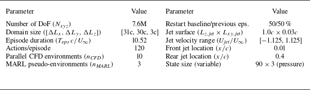
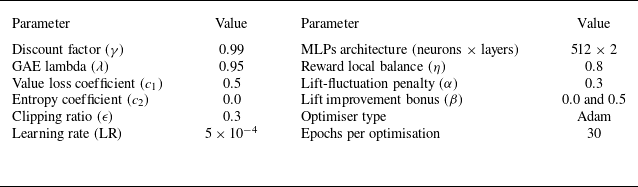

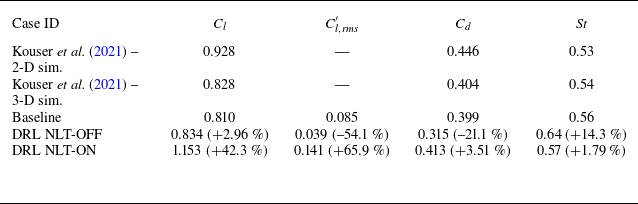

 5U∞/c


 Qc2/U∞2=0.1

 z
 ωzc/U∞∈[−10,10]
 x
 y

 +
 +
 +
 ×

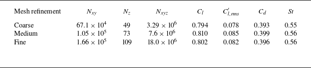

 Δt∗
 Δt∗=(tend−t)U∞/c
 ϕ(Δt∗)=(1/Δt∗)∫0Δt∗ϕ(t)dt

 Lz/c
 Nxyz


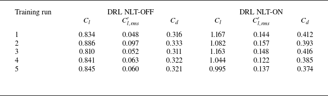

 μ
 σ


 Open access

