1. Introduction
Considerable attention has been focused recently on developing a US cap-and-trade system for greenhouse gases (GHG). New proposals in the US Congress specify a relatively long horizon – through 2050 – on the basis that this would provide greater certainty for investment and planning purposes, and this naturally focuses attention on the role of expectations. Other issues related to greenhouse gas abatement policy, such as the effects on growth of using CO2 auction to revenue to reduce taxes on capital or labor, banking and borrowing, or action in anticipation of a policy going into effect also depend on people looking forward and acting differently today because of something that will happen in the future. To fully investigate these issues requires a model where the knowledge of future events is reflected in current decisions. Here we apply a forward-looking dynamic version of the Emissions Prediction and Policy Analysis (EPPA) model to examine US GHG cap-and-trade measures that approximate recent bills under consideration in the US Congress. A recursive dynamic version of EPPA (Paltsev et al., Reference Paltsev, Reilly, Jacoby, Eckaus, McFarland, Sarofim, Asadoorian and Babiker2005) has been used to conduct similar analysis (Paltsev et al., Reference Paltsev, Reilly, Jacoby, Gurgel, Metcalf, Sokolov and Holak2008). A main interest here is to compare the behavior of the forward-looking and recursive versions, especially with regard to those issues where expectations are particularly important.
The paper is organized in the following way. In the next section, we briefly describe the forward-looking model used. Section 3 sets out the policy scenarios we investigate, section 4 reports the results of our investigation with the forward-looking model, comparing them with results from the recursive model where useful, and section 5 offers some conclusions.
2. The model
The EPPA model is a multisector, multiregion computable general equilibrium (CGE) model of the world, which represents the circular flow of goods and services in the economy, including the representation of production technologies, trade flows, parameters and greenhouse gas inventories (Paltsev et al., Reference Paltsev, Reilly, Jacoby, Eckaus, McFarland, Sarofim, Asadoorian and Babiker2005). It provides projections of world economic development and emissions along with analysis of proposed emissions control measures. It is used to analyze the processes that produce greenhouse-relevant emissions and to assess the consequences of policy proposals, providing estimates of the magnitude and distribution among nations of their costs and clarifying the ways that changes are mediated through international trade.
The formulation of the model adopts the Arrow–Debreu framework, where the competitive equilibrium is determined by optimization decisions of consumers and producers. Each region of the model has a representative agent which maximizes welfare through the allocation of income across consumption of goods and services, and each producing sector in the economy is represented by a firm which chooses primary factors and intermediate inputs to maximize profits given its technology. The model has a complete representation of markets, which all clear simultaneously in equilibrium. The benchmark equilibrium is calibrated to match Global Trade Analysis Project (GTAP) data (Hertel, Reference Hertel1997; Dimaranan and McDougall, Reference Dimaranan and McDougall2002) augmented by data on the emissions of greenhouse gases, aerosols and other relevant species, taxes, and details of selected economic sectors. Provision is made for analysis of uncertainty in key human influences, such as the growth of population and economic activity and the pace and direction of technical advance. The model solves in 5-year intervals starting at 2005.Footnote 1
2.1. EPPA: forward-looking version
A forward-looking dynamic general equilibrium model optimizes decisions both within a time period (across sectors, regions, goods, and inputs) and across time periods whereas a recursive dynamic model only optimizes decisions within a time period.
Solving the forward-looking model is computationally demanding because the solution requires simultaneous consideration of all time periods, and some simplifications from the recursive dynamic version are required. The forward-looking version applied here simplifies the EPPA structure in three ways: (a) instead of the 16 regions of the recursive dynamic version, we collapse the model to two regions, the United States and the Rest of the World (ROW);Footnote 2 (b) the model horizon is shortened from 2100 to 2050; and (c) the capital vintage structure is simplified and we do not include adjustment costs associated with rapid expansion of new technologies.
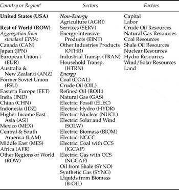
In other ways the model is unchanged from the standard EPPA with the same technological detail as shown in table 1. The underlying GTAP data (Hertel, Reference Hertel1997; Dimaranan and McDougall, Reference Dimaranan and McDougall2002), characterization of alternative technologies, elasticities of substitution, and the like are generally unchanged from the recursive version of the model. The exceptions are two. First, given our interest in comparing the response to GHG policy between the models, we benchmark the reference projection of the forward-looking model to match that of the recursive in terms of GDP growth and GHG emissions. Labor productivity and autonomous energy efficiency improvement are adjusted in this benchmarking process. Second, aggregation of the regions in the recursive model to a single ROW region leads to a different response even if parameterization is identical across regions. We have made an effort to make the ROW behave broadly similarly to the aggregated regions in the recursive model. Since our primary interest here is the response of the US to climate policy, any differences in ROW response would affect US response only indirectly through the international trade and capital accounts.
Regions, sectors and primary factors in the EPPA model

aSpecific detail on regional groupings used to define the ROW region is provided in Paltsev et al. (Reference Paltsev, Reilly, Jacoby, Eckaus, McFarland, Sarofim, Asadoorian and Babiker2005).
2.2. Equilibrium structure and dynamic process
The forward-looking dynamic EPPA model is conceptually built on the classical Ramsey economic growth approach. In this way, the model attempts to represent infinite lived agents who maximize the present value of welfare from consumption, considering the trade-off between present and future consumption.Footnote 3 Nevertheless, unlike some of the conventional applications of the Ramsey formulation,Footnote 4 the forward-looking EPPA model is multiregional and does not assume balanced growth paths, i.e., economic growth rates are allowed to vary across regions and over time. This latter feature is particularly crucial in applied modeling work since in the real world countries are usually not on steady growth paths and hence it is important that an applied model allow for both transitional dynamics and catch-up across regions.Footnote 5
The most important difference between the recursive and forward-looking versions of EPPA is the optimization process. In the forward-looking model, a representative agent allocates income across consumption in different time periods in order to maximize welfare,Footnote 6 which means, in each single period, the representative agent must choose between current and future consumption. Future consumption is purchased through savings. The intertemporal allocation of consumption is governed by a rate of time preference between current and future consumption. The solution of the optimization problem generates an equilibrium where a unit of consumption today is as valuable as one unit of consumption (adjusted for time preference) in the future.
2.3. The intertemporal optimization problem
Here we represent the basic theoretical structure that underlies the forward-looking model. We focus on the general mathematical representation as it relates to reformulating the problem as a forward-looking model and suppress other details of the EPPA model that are unchanged from the recursive formulation.Footnote 7 The utility function employed in the forward-looking EPPA is a constant intertemporal elasticity of substitution function. The representative agent in each region maximizes this utility function, subject to a budget constraint, technology and the evolution of capital stock in the economy. The representative agent in each region is endowed with an initial stock of capital, labor, and energy resources. Set r denotes the different regions and set t denotes time. Equation (1) represents the utility function:

where Qrt is a combination of aggregate consumption and leisure in region r and time t, ρ is a time preference or discount rate and θ is the inverse of the elasticity of intertemporal substitution. This formulation makes labor supply decisions endogenous. We use the term ‘full consumption’ to refer to Qrt, which is represented as:

where Crt is the aggregate consumption at region r and time t, Zrt represents leisure time at region r and time t, α is the weight of consumption in full consumption and 1/(1 − ϕ) is the elasticity of substitution between consumption and leisure.Footnote 8
The budget constraint can be thought of as the balance of income and expenditure over the horizon, represented by equation (3):Footnote 9

where pCrt is the price of aggregate consumption at region r and time t, wrt is the wage rate, Lrt is the labor endowment in efficiency units, pK r0 is the initial price of a unit of capital, K r0 is the initial stock of capital, p T+1 is the price of the post-terminal capital, and K T+1 is the stock of capital in period T+1. All prices are discounted, i.e., they are present value prices.
The lifetime budget constraint means that the present value of full consumption should be equal to the present value of wage income and the initial value of capital stock less the value of post-terminal capital.
At each period t, an imbalance in a region's budget constraint accounts for capital flows (or foreign savings and investments) among regions, which may be interpreted as real assets in terms of a CGE model. In other words, capital flows are allowed among regions, in response to differences in real rate of returns. Thus the closure of the model regarding the balance of payments requires that capital flows cover the current account deficit (or surplus), and they also should be equal to the differences between aggregate expenditures (private and public consumption plus investments) and aggregate income (returns to labor, capital, energy resources and tax revenue). This condition can be represented as:

where kflowrt is the capital flow to region r at time t, pIrt is the price of a unit of investment and rKrt is the rental price of capital.
This closure rule requires that any current account deficit in one country must be compensated by current account surpluses elsewhere. In addition, this closure rule means that in every region any excess of aggregate expenditure over aggregate income today should be paid off by the region in the future. Thus, it requires no net change in foreign indebtedness over the model horizon. These conditions can be represented by the following relations:

From equation (3) we can also derive the condition where the rate of return over the assets the agents possess today determines the value of assets tomorrow:

where rt is the real interest rate at time t.
This foreign trade closure rule allows countries to temporarily have foreign accounts imbalanced in response to, for example, a greenhouse gas mitigation policy, as long as that imbalance is made up for in later years. The recursive EPPA fixes the foreign accounts gradually phasing out any existing capital account imbalance. This feature of the forward-looking model provides another avenue of adjustment that is not available to agents in the recursive model.
Physical capital in the forward-looking model evolves in the economy through the creation of new capital from investments, considering a constant depreciation rate at each period. The capital accumulation equation is represented by (7):

where δ represents the depreciation rate.
The maximization of (1) subject to (3), (4), and (7),Footnote 10 considering initial zero capital flows as a simplification, generates first-order conditions:


where prt represents the price of aggregate output, ηrt is the price of leisure, pKrt is the price of one unit of capital stock at period t, and pK r,t+1 is the price of one unit of capital stock at period t + 1. These prices arise as Lagrange multipliers (shadow prices).
In the forward-looking dynamic EPPA model, the above optimization problem is converted into a market equilibrium formulation using the mixed complementarity problem (MCP) algorithm (Mathiesen, Reference Mathiesen1985; Rutherford, Reference Rutherford1995), and solved numerically using the General Algebraic Modeling System (GAMS) software (Brooke et al., Reference Brooke, Kendrick, Meeraus and Raman1998).Footnote 11
2.4. The infinite horizon and the terminal condition
The optimization problem posed by the numerical model is necessarily restricted to a finite horizon. An issue that arises is that the representative agent has no incentive to accumulate capital in the final period, and thus has the tendency to consume all income in the last period of the model, with investment equal to zero. Moreover, this result would have repercussions for earlier periods as agents looked forward and saw that the value of investment was reduced because it was only being used through the terminal year. The solution is to impose a terminal condition in the last period of the model that requires the representative agent to continue to save and invest. The objective is to set the terminal condition such that it approximates the level of investment in the terminal period that would be obtained in the infinite horizon problem. In this way, the solution of the finite horizon problem is very close to the solution of the infinite horizon problem.
The terminal condition we use assigns a post-terminal growth rate to investments. The growth rate of investment in the terminal period is required to be equal to the growth rate of consumption in that period, as shown by the equation:

The equilibrium condition of the infinite horizon problem is balanced growth – the economy and all sectors growing at the same constant rate. As described by Rutherford (Reference Rutherford1998), this condition assures a balanced investment growth without imposing a specific capital stock target or a specific exogenous growth rate in the post-terminal period. It means that, after a policy shock, the model can determine a different growth path. With an exogenously specified rate of growth of investment in the final period, the model would be forced to return to that growth rate by the end of the period, and that would have consequences for estimates of policy costs in earlier years. Another approach to solving a numerical model of this type is to extend the horizon of the model far beyond the period of interest so that a relatively arbitrary terminal condition, while affecting the solution of years leading up to the terminal year, has little or no effect on the period of interest. However, if the period of interest is the next 70 or 100 years, the model horizon might need to be extended to 200 years in the future in this method, greatly increasing the computational demands.
Comparison of policies that have different implications for growth can also require evaluation of welfare difference in the post-terminal period. If the horizon is long enough, the discounted value of these difference may be unimportant, but experimentation with the model showed significant differences when the horizon was truncated to 50 to 70 years. We thus create an index that includes an estimate of the infinite horizon welfare as follows. First we formulate the aggregate index as a two-period problem, the period from present to the model horizon, and the period beyond the horizon of the model,

where θ is, as defined previously, the inverse of the elasticity of intertemporal substitution, Welfare is defined as the welfare index over the infinite horizon, U is lifetime welfare over the horizon of the model, and UT is the annual welfare in the last period (T) of the model that with an appropriate estimate of β, the share weight of the post-horizon welfare, is used to approximate welfare in the post-T period. For interest rate r we approximate β by using the GDP growth rate (g) in the formula:

where

The first term of the numerator of (15) is the final period growth discounted from T to today. This discount factor is multiplied times the discounted growth factor from T to infinity. The denominator is the sum of growth over the horizon (t = 0 to T) plus the numerator.
2.5. Calibration
The calibration of the forward-looking EPPA model follows in several ways the same process as version 4 of the recursive model (EPPA 4). In common with the recursive version of EPPA is that we start with base year data for 1997. However, in a forward-looking model, policy shocks in the future will change results in any simulated year. Thus, for example, a policy beginning in 2010 would change the economy in 2000 and 2005 compared with a reference case if we treated these years as forecast years. To avoid this rewriting of history with every policy simulation, we use the model in an initial calibration phase to project a simulated benchmark data set for 2005 that matches approximately the recursive dynamic model, which itself has been benchmarked to historical data for these years. Then in further simulations of the forward-looking model we use the simulated year 2005 effectively as the base year of the model. The first simulation year is 2010. This assures that under a policy scenario the economy does not begin adjusting to the policy in what is, in reality, the past.
The most important aspect of the calibration of the forward-looking model, however, is the consistency among capital stock, capital earnings, investment, the interest rate, the growth rate of the economy, and the rate of depreciation. Key relationships among those variables are important in determining the growth path. While investment, savings and returns to capital are included in the benchmark data base, the data do not include measures of the capital stock or depreciation. The goal of benchmarking a dynamic CGE is to establish conditions along an equilibrium growth path. We follow the convention of Rasmussen and Rutherford (Reference Rasmussen and Rutherford2004), Cretegny and Rutherford (Reference Cretegny and Rutherford2004), and Sue Wing and Popp (Reference Sue Wing, Popp, Hanneman and Farrell2006) and establish a long-run rate of return and a depreciation rate, which together with the observables implies a capital stock and investments, using the first-order conditions for these variables from equations (8) to (10). In this simple formulation, an average rate of return and depreciation rate must be used to reflect a wide range of assets with different risks and depreciation rates. We recognize that investment, savings, and returns to capital for the benchmark year may not be consistent with an equilibrium growth because of business cycles, and we check the implied capital stock and capital-output ratio for consistency with other measures, and further adjust the data and parameters as needed to generate a projected near-term growth path consistent with recent history. The projected growth path is quite sensitive to the relationship of these parameters and comparing the rate to history is a good check on these assumptions. Given that neither the capital stock nor the depreciation rate is accurately measured, there is inevitable uncertainty in these estimates.Footnote 12
We start by assuming the real interest rate is 4 per cent per year, a value consistent with observed rates of return. From (9) and (10) we can determine the initial level of the price of one unit of capital (we omit set r to facilitate the notation):

Assuming a 5 per cent depreciation rate per year in the US and ROW, the initial rental price of capital can be found by substituting the values of pKt, pK t+1, pt and p t+1 from equation (16) into equation (8) to obtain:

Based on the returns to capital (or capital earnings) observed in the base year (RK 0), the capital stock can be obtained from:

We then calculate the investment level that is consistent with depreciation and a benchmark growth rate of the economy. Thus, the total investment at the initial period can be calculated as:

where g is the benchmark growth rate of the economy. The benchmark growth is an ‘average’ growth rate for the initial period, recognizing that growth in any single year may be distorted by business cycle behavior of the economy. Note also that I 0 is likely inconsistent with observed investment in the initial year. Thus, we adjust the initial investment level in the data to be equal to I 0, balancing the initial accounts with a corresponding change to the endowment of the representative agent. This assures that the growth rate in early periods will be consistent with recent observation.
Finally, it is necessary to define the value of the intertemporal elasticity of substitution in equation (1) and the time preference parameter (ρ). We adopt the value of 0.5 as the inter-temporal elasticity of substitution. The time preference parameter is then determined as:Footnote 13

3. Reference and policy scenarios
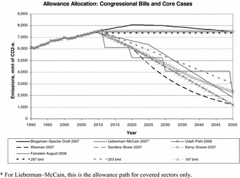
Given our desire to compare results with the recursive version of EPPA (Paltsev et al., Reference Paltsev, Reilly, Jacoby, Gurgel, Metcalf, Sokolov and Holak2008), we have adopted the same three core policy scenarios, shown in figure 1, which bracket the allowance paths specified in the Congressional proposals. In terms of the policy cost implications, a good summary measure of the different proposals is the total number of tons of CO2-equivalent greenhouse gases they would allow from 2012 to 2050. These core cases are 287 billion metric tons (bmt),Footnote 14 203 bmt, and 167 bmt, and we use these as labels to designate the scenario results. Because we have an aggregate region ROW, we are not able to represent different policies in different parts of the world as in Paltsev et al. (Reference Paltsev, Reilly, Jacoby, Gurgel, Metcalf, Sokolov and Holak2008). Instead we impose the ROW abatement from reference emissions taken from the recursive simulations for the regions that make up the ROW. For the recursive simulations we assumed Europe, Japan, Canada and Australia/New Zealand adopted a policy in 2015 that gradually brought them to 50 per cent below 1990. Other regions had no policy until 2025, when emissions were then capped at 2015 levels. That cap was tightened further to return to year 2000 level emissions in 2035. An obvious limitation of the aggregate region ROW is that, implicitly, there is an ROW-wide cap in place throughout the 2015–2050 period. Thus, the cuts in the developed regions in early years can be spread across the ROW. This could affect some of the terms of trade results. For example, a relatively tighter policy in a limited number of regions could transmit terms of trade effects to the US and that could shift trading patterns with other regions that had no policy. Such a response would not be picked up in the two-region model.
Scenarios of allowance allocation over time

As with the recursive simulations, for the core cases we assume that all GHGs and all sectors are included in the policy, and that allowances (or any revenues) are distributed in a lump sum manner. We simulate emissions banking (i.e., an ability to use emissions allowances in the periods later than those when they are issued) in the US, but as in the recursive simulations we do not allow banking in the ROW region. This procedure captures some aspects of the fact that some regions are not participating in early periods; i.e., if we allow banking, it would imply that developing countries abate in the 2015–2025 period and bank for later years, but without banking the aggregate ROW time path of abatement is consistent with the recursive results and delayed entry of developing countries. We also simulate one of the core cases (203 bmt) without banking and borrowing of permits in the US to be able to capture the importance of the forward-looking behavior on it.
4. Results
4.1. Comparison of model results for the core cases
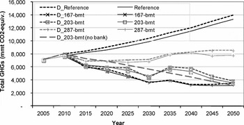
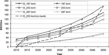
The recursive and forward-looking versions of the EPPA model were designed to be as close as possible in terms of GHG emissions by benchmarking them in the reference case. Figure 2 compares GHG emissions from the two versions in the reference and core policy cases, and figure 3 shows the associated CO2-e prices. In the recursive-dynamic simulations we set CO2-e prices to rise at the discount rate to approximate emissions banking behavior. In the forward-looking model, the CO2-e price path is a result of an explicit optimization rather than a predetermined path imposed to approximate optimization behavior. A comparison of results of the two versions of the model in figures 2 and 3 suggests that this approximation in a recursive-dynamic EPPA model works very well in terms of the timing of abatement. Both versions yield very similar paths of emissions and CO2-e prices under the policy scenarios. The policy-related results are not due to benchmarking, rather the results are similar because of a similar production and consumption structure of the models.
GHG emissions in the forward-looking (dashed lines) and recursive (solid lines) models

CO2-e prices in the forward-looking (dashed lines) and recursive (solid lines) models

The no-banking case highlights how the banking behavior saves allowances in the first half of the policy horizon and allocates many more allowances to the second half of it.Footnote 15 In this case, CO2 prices do not exhibit a particular pattern, since abatement opportunities do not follow the allowances distribution. Carbon prices are cheaper in the initial years since emissions cuts are relatively lower and cheaper to perform, but as the emissions constraints get higher, carbon prices rise faster than in the banking case, reaching much higher levels at the end of the model horizon. As the rest of the world adopts a stronger policy around 2035, terms of trade become favorable to the US and carbon prices do not increase that fast for a while. At the end of the horizon, carbon prices are much higher under a no-banking policy.
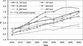
Alternative assumptions about expectations as represented in the two model versions do, however, lead to a difference in the welfare results. An important phenomenon represented in forward-looking models is consumption shifting: people look ahead to see relatively abrupt changes in consumption and try to avoid these shocks by smoothing consumption through time. Figure 4 shows this response. In the recursive-dynamic model, the changes in policies abroad create shocks to US consumption through unexpected changes in the terms of trade. In the forward-looking model, those consumption shocks are smoothed out. Also, note that consumption changes occur in the forward-looking model in 2010 even though the policy is not implemented until 2015. Agents in the model are looking forward and know the policy is coming. They modify their consumption behavior immediately. In this case, looking forward and realizing that consumption will be more expensive in the future, agents increase their consumption in 2010. The result is a consumption gain (shown as negative consumption losses in figure 4) before the policy goes into effect. Consumption losses are higher as we approach the end of the model horizon under a no-banking policy, since agents can only adjust their consumption path, while in the banking case agents have more flexibility, adjusting allowances and consumption.
Annual consumption loss in the forward-looking (dashed lines) and recursive (solid lines) models

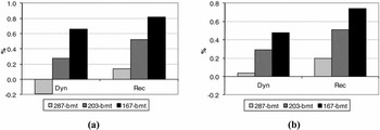
In a forward-looking model, economic agents are represented as optimizing over time as well as within any period; we therefore expect the welfare cost of any policy to be less in the forward-looking than in the recursive model. In figure 4 the time path of consumption loss is lower for most periods in the dynamic than in the recursive model, although the price of emissions is similar in the two models. Figure 5a shows that the lifetime welfare change is lower for the dynamic model. Lifetime welfare is computed automatically in the forward-looking model and for the recursive model we calculate the net present value (NPV) change using a 4 per cent discount rate consistent with the interest rate in the forward-looking model. The forward-looking model trims about 0.10 to 0.25 percentage points from the welfare loss estimates of the recursive model. Note also that for the 287 bmt case, the lifetime welfare change is a benefit for the US. This apparent benefit results from the anticipation of the terms of trade effects from the ROW region taking on a more stringent policy relative to the US. Figure 5b shows that there are net welfare losses for the US in the 287 bmt case if GHG controls are implemented by the US only. In this case losses are shown by both model versions. Paltsev et al. (Reference Paltsev, Reilly, Jacoby, Gurgel, Metcalf, Sokolov and Holak2008) showed similar terms of trade benefits in the recursive model from implementation of the policy abroad. However, because the abatement costs within the US were somewhat higher, the terms of trade benefit was not enough to create a net benefit to the US with the recursive model.Footnote 16
Lifetime welfare change: (a) forward-looking (Dyn) and recursive (Rec) models; (b) when GHG controls are implemented by United States only, forward-looking (Dyn) and recursive (Rec) models

4.2. Early action abatement
One aspect of forward-looking behavior is that, once agents know mitigation measures are coming, they would like to begin abating immediately so long as they can bank allowances for use once the emissions cap goes into effect. Such early abatement can reduce the overall policy cost while achieving the same level of cumulative emissions. Emissions during the policy period (2015–2050) will be somewhat higher, made up for by lower emissions prior to 2015. Many of the Congressional proposals include the possibility of such ‘early action credits’. Table 2 presents the impacts on emissions in 2010 with and without early action crediting. Without early action credits there are two effects leading in opposite directions. One is the substitution effect on consumption in 2010 knowing that the real price of consumption will rise once the policy is in place, which should increase pre-implementation emissions. The other, given vintaging, is an incentive to invest in lower emitting technology before the policy is in place or otherwise be stuck with uneconomic capital once the policy comes into effect. We find that latter effect dominating so that there is a slight reduction in emissions in 2010 even without early action crediting. It may be that this would be stronger if we were able to vintage the capital stock more completely.
GHG emissions (mmt CO2-e) in 2010 with and without early action credits

Source: Model results.
With early action crediting we get substantial reductions in 2010 – a 10 per cent to nearly 20 per cent reduction. To create early action credits in reality requires a rather cumbersome effort to establish a baseline level of emissions for those agents who want to claim such credits. To the extent that the baseline is too generous, credits beyond any real abatement may be granted. On the other hand, if the early action crediting process is narrowly defined to avoid granting credits unless there is certainly real abatement, then many opportunities for abatement may be excluded. The nature of the simulation implies that issues of establishing baselines are ideally resolved so it is as if the cap policy began in 2010, and so cannot take into account some of the well-known difficulties of such crediting systems. The 10–20 per cent should thus be seen as an upper limit on real reductions that could be achieved through early action crediting.
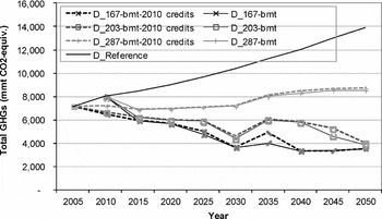
Even with the fairly substantial reductions from early action in 2010, figure 6 illustrates that it does not have that much effect on the overall abatement level throughout the period. The obvious reason is that abatement during the five-year period represented by 2010 is spread over the entire 2012 to 2050 period. The effect of early action on CO2-e prices and welfare costs are not shown here but are barely discernible in a graphical representation. Thus, from economic efficiency grounds, not much is gained from an early action credit program, even though quite a lot of effort has gone into defining such programs. The risk with them is that if the baselines are not carefully defined, and a lot of credits are forthcoming, they may be little more than hot air.
Early action credits; allowed (dashed lines), not allowed (solid lines)

4.3. Revenue recycling with forward expectations
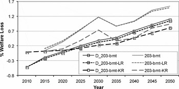
Another area where we might expect the forward-looking model to generate results different from a recursive version is in the effects of revenue recycling. Using the 203 bmt case as an example, we compare the forward-looking results with those from the recursive model (figure 7). Both show relatively little effect of reducing the labor tax rate, however, the forward-looking results are positive and accumulate whereas the recursive results show almost nothing. The capital income tax recycling results show strong effects on growth in both cases. In the forward-looking model, however, additional consumption losses in early years occur as consumption is reduced so that saving and investment can be increased to take advantage of the capital tax cut. Because in the recursive model savings do not respond to investment demand, we instead introduced market capital and residential capital, recognizing that most residential capital (i.e., investment in owner-occupied homes) is not subject to capital income taxation.Footnote 17 This follows an approach that Bovenberg et al. (Reference Bovenberg, Goulder and Gurney2005) applied in a static setting. Although the recursive representation of household capital needs more refinements, these experiments suggest that it may be useful to consider residential capital as another source for funding increased investment in response to a capital tax cut in the forward model. Being able to shift to more market investment from residential investment appears to make it possible to fund an increase in market investment without the big penalty on near-term consumption. Whether this result would hold up in the forward-looking model needs to be seen.
Annual consumption changes with revenue recycling to labor taxes (LR) or capital taxes (KR), recursive and forward-looking model

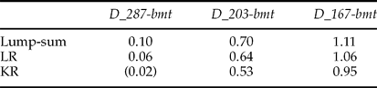
For comparing welfare change with the recursive model, we have used a lifetime welfare change that is computed only over the model horizon. Lifetime welfare in the recursive model is computed as simply the NPV change in the annual welfare using a comparable 4 per cent discount rate. In comparing lifetime welfare computed this way for capital and labor tax recycling, we found little difference between them. The big consumption losses in early years with capital tax recycling were offsetting discounted gains from future years but the growing gain from capital tax recycling – the growth effect – suggested that the finite horizon welfare measure could be misleading. The infinite horizon approximations of the welfare gains from the policies, following the approach described in section 2.4, are shown in table 3. This comparison shows that capital tax recycling improves welfare somewhat more than labor tax recycling. For the 203 bmt case, for example, the lifetime welfare cost without recycling is 0.7 per cent, with capital tax recycling it is 0.53 per cent, and with labor tax recycling it is 0.64 per cent. The small benefits of labor tax recycling in all years end up generating substantial lifetime welfare benefits, but they are not as large as with capital recycling where welfare losses in initial years are offset by substantial gains in consumption occurring in later years. The apparent ‘strong double-dividend’ effect of capital tax recycling in the 287 bmt case again results from terms of trade effects from abroad. When there is no policy abroad there is a welfare loss.
Welfare losses over the infinite horizon with labor (LR) and capital (KR) recycling in the forward-looking model

Source: Model results.
One aspect of these results is that the absolute gain from revenue recycling is about the same in all three cases. The reason for this is that the auction revenue, and thus the tax cut, is similar in all three cases. The 167 bmt case generates much higher allowance prices but because the number of allowances is falling over time the auction revenue begins to fall. If the long-term policy goal is stabilization of concentrations, allowable emissions must fall very low, and auction revenue would drop off, and in that case revenue-recycling benefits would eventually fall because there would be little revenue available.
5. Conclusion
A forward-looking version of a CGE model is a useful tool to analyze situations where economic agents can look forward and anticipate future changes in economic policy and available technology. In this paper we apply a forward-looking dynamic version of the Emissions Prediction and Policy Analysis recursive dynamic model to examine US GHG cap-and-trade measures that approximate recent bills under consideration in the US Congress. For numerical reasons, a forward-looking version of the EPPA model must be simplified in a number of ways. We have tried to retain key features such as vintaging and technology detail. By retaining the similar structure of the model, we are able to compare results of the two versions and see how the forward-looking solution changes key results when applied to an environmental policy constraint.
Our results indicate that the forward-looking and recursive versions produce very similar CO2-e prices and abatement paths when we assume a carbon price raising at the discount rate in the recursive model. This result leads us to conclude that the way that dynamics is introduced in the recursive EPPA model appears to approximate well the forward-looking result in terms of prices and emissions profiles. This is reassuring to the extent that the longer horizon and multiregion recursive structure is necessary because the forward-looking EPPA model of that complexity cannot be solved – some basic results obtained from the recursive structure can be considered fairly robust regardless of whether solved in a recursive or fully dynamic fashion. Our conclusion about similarity of the results should be treated with appropriate caution. We do not claim that recursive and forward-looking models always produce similar results. Our findings simply show that with a proper formulation for capital accumulation and emissions banking behavior that leads to a certain carbon price path, the recursive-dynamic and forward-looking versions can produce similar results.
Estimates of welfare diverge as one might expect – we see consumption smoothing in the forward-looking model and the additional flexibility of optimizing over time reduces the welfare cost compared with the recursive model. In terms of policy relevance, one might question whether the assumption of perfect foresight moves us closer to or farther from reality in estimating policy costs. Pervasive uncertainty, likely revision of policies over time, and unexpected changes in technology suggest the need for a stochastic solution but solving a complex CGE model stochastically is currently beyond available computational resources.
However, for some economic problems that depend critically on expectations, the forward-looking solution is necessary in order to better understand economic behavior. We examined two issues: revenue recycling and early action credits. With regard to revenue recycling we found that capital tax recycling reduces cost more than labor recycling, and the time path of benefits with capital tax recycling is much different than for labor tax recycling. Consumption in early years falls as more consumption is devoted to savings and investment, and so the capital tax policy is essentially a growth policy where agents give up consumption today for greater consumption in the future. The labor tax recycling benefit is due more to a static reallocation of resources. With regard to early action credits, we find that such provisions, for the policy considered, could reduce pre-implementation emissions by 10 to almost 20 per cent. This is a substantial reduction relative to current emissions, but it ends up not having much effect on the overall cost of the policy because the banking of these credits is then spread over a long horizon. We do not find extra emissions in anticipation of the policy without early action credits; this is not surprising given the increase in the real price of consumption once the policy starts. If anything, we see a slight reduction with reference to 2010 as investment decisions anticipate the value of lower emitting technology in the future.
Finally, there are several limitations and challenges associated with the forward-looking modeling of climate policies. It is necessary to reduce the model dimensions to solve it. We do this by, among other things, dropping the full vintaging of the capital stock and considering fewer explicit technological options. The estimation of a lifetime welfare index may be misleading if the policy being simulated increases investments in early years and shifts consumption towards the end of the model horizon, since much of the gains would be observed in the post-terminal period. The assumption of perfect foresight does not guarantee a closer move toward reality in estimating policy costs. A stochastic solution should be better to deal with pervasive uncertainty, but solving a complex CGE model stochastically is currently beyond available computational resources. Other aspects not being considered in the current analysis include the potential shifts in technology due to climate change policy and also distributional impacts, both of which might affect the welfare effects.