Introduction
One of the most crucial resources for crop production is soil water, which is impacted by the soil, topography, vegetation, hydrology and climatic factors (Saue and Kadaja, Reference Saue and Kadaja2014). The soil moisture (SM) content available to plants depends on infiltrated precipitation or irrigation and the capillary rise of groundwater to the root zone, whereas the soil evaporation, drainage, runoff and plant transpiration reduce it (Allen et al., Reference Allen, Pereira, Raes and Smith1998). Furthermore, the physical properties of soil, such as the soil pore size distribution, soil texture and structure, which can be modified by human interactions such as soil cultivation, affect the total and crop-available soil water holding capacity (Fry and Guber, Reference Fry and Guber2020). A major cause of yield reductions or even crop failures in Central Europe is the insufficient availability of soil water during the growing season. These events occur mainly during the summer months (Eitzinger et al., Reference Eitzinger, Trnka, Semeradova, Thaler, Svobodová, Hlavinka, Šiska, Takac, Malatinska, Novakova, Dubrovsky and Žalud2012a; Thaler et al., Reference Thaler, Eitzinger, Trnka and Dubrovsky2012), with a rising trend, especially in the April‒June period (Trnka et al., Reference Trnka, Hlavinka, Mozny, Semeradova, Stepanek, Balek, Bartosova, Zahradnícek, Blahova, Skalak, Farda, Hayes, Svoboda, Wagner, Eitzinger, Fischer and Zalud2020). In the coming decades, droughts are expected to be more frequent and severe over the growing season in these regions as a result of a changing climate (Grillakis, Reference Grillakis2019; Jia et al., Reference Jia, Shevliakova, Artaxo, De Noblet-Ducoudré, Houghton, House, Kitajima, Lennard, Popp, Sirin, Sukumar, Verchot, Shukla, Skea, Calvo Buendia, Masson-Delmotte, Pörtner, Roberts, Zhai, Slade, Connors, van Diemen, Ferrat, Haughey, Luz, Neogi, Pathak, Petzold, Portugal Pereira, Vyas, Huntley, Kissick, Belkacemi and Malley2019; Hari et al., Reference Hari, Rakovec, Markonis, Hanel and Kumar2020; Büntgen et al., Reference Büntgen, Urban, Krusic, Rybníček, Kolář, Kyncl, Ač, Koňasová, Čáslavský, Esper, Wagner, Saurer, Tegel, Dobrovolný, Cherubini, Reinig and Trnka2021; Ercin et al., Reference Ercin, Veldkamp and Hunink2021; Trnka et al., Reference Trnka, Vizina, Hanel, Balek, Fischer, Hlavinka, Semerádová, Stepánek, Zahradnícek, Skalák, Eitzinger, Dubrovsky, Máca, Belínová, Zeman and Brázdil2022).
Importantly, the available soil water content is highly variable both temporally and spatially (Zhang et al., Reference Zhang, Li, Sun, Zhang, Liu, Wang and Li2022) because of the considerable spatial variability in soil physical properties (Vanderlinden et al., Reference Vanderlinden, Giráldez and Van Meirvenne2005). For precision agriculture applications, for example, monitoring the spatial variability of SM at very high resolution would be highly beneficial, e.g. for increased irrigation efficiency and related crop water productivity (Vuolo et al., Reference Vuolo, Essl, Zappa, Sandén and Spiegel2017).
Currently, four different approaches are used to estimate SM for precision farming applications in croplands: direct in-situ measurements using methods such as time-domain reflectometry (TDR) (Walker et al., Reference Walker, Willgoose and Kalma2004); remote-sensing techniques involving the use of microwave, optical and thermal sensors (Rahimzadeh-Bajgiran and Berg, Reference Rahimzadeh-Bajgiran, Berg, Srivastava, Petropoulos and Kerr2016); non-invasive geophysical methods (Bogena et al., Reference Bogena, Huisman, Güntner, Hübner, Kusche, Jonard, Vey and Vereecken2015; Garré et al., Reference Garré, Hyndman, Mary and Werban2021) and soil‒crop water balance modelling approaches, which are based on observed weather data (Pereira et al., Reference Pereira, Paredes and Jovanovic2020).
Measuring the in-situ SM for different cropping systems, soils and environments is relatively costly, labour-intensive and time-consuming (Kivi et al., Reference Kivi, Vergopolan and Dokoohaki2022) but is indispensable for the calibration and validation of satellite-based SM measurements, ground non-invasive geophysical methods and soil water balance models (Dorigo et al., Reference Dorigo, Wagner, Hohensinn, Hahn, Paulik, Xaver, Gruber, Drusch, Mecklenburg, van Oevelen, Robock and Jackson2011). Most in-situ measurements and networks offer only low spatial representativeness. However, frequent point measurements of SM or networks of multiple stations demand high maintenance effort, which is associated with high economic costs and personnel input (Brocca et al., Reference Brocca, Ciabatta, Massari, Camici and Tarpanelli2017).
The use of remote-sensing-based SM products over various spatial scales has been successfully applied to large areas. Here, microwave observations, either from passive or active sensors, are the most common method for measuring surface SM. The benefit of microwave remote sensing for SM estimates is the comparatively high spatio-temporal coverage in relation to cost (Brocca et al., Reference Brocca, Ciabatta, Massari, Camici and Tarpanelli2017; Akash et al., Reference Akash, Mohan Kumar, Bhaskar, Deepthi and Sukhdev2024). However, the accuracy is lower than that of in-situ measurements since remote-sensing applications for SM are limited by the spatial resolution of the footprint (>10 km for most sensors except for synthetic aperture radar [SAR]), the shallow penetration depth of the upper soil layer (2–7 cm) and quality issues in mountainous terrain, heavily vegetated areas and other specific surface conditions (Brocca et al., Reference Brocca, Ciabatta, Massari, Camici and Tarpanelli2017). At high resolutions, such as those obtained from Sentinel-1 SAR observations, soil roughness and the structure of vegetation may affect SM retrievals even more strongly than at coarse spatial scales (Vreugdenhil et al., Reference Vreugdenhil, Wagner, Bauer-Marschallinger, Pfeil, Teubner, Rüdiger and Strauss2018). Nonetheless, the high spatio-temporal coverage of remote-sensing systems cannot be reached with in-situ measurements but provides valuable insights into the large-scale dynamics of soil water fluxes. In addition to microwave sensors, thermal infrared remote-sensing methods (TIRs) are also used to determine SM indirectly by assessing temperature variations (Gojiya et al., Reference Gojiya, Rank, Chauhan, Patel, Satasiya and Girish2023). While their relatively high-spatial (e.g. Landsat: 30 m, Sentinel-2: 10–20 m) and -temporal (e.g. Sentinel-2 every few days; Landsat with a 16-day revisit cycle) resolutions together with long-term coverage are advantages, TIR surface penetration is minimal at 1 mm and can be further limited by the density of vegetation (Rahimzadeh-Bajgiran and Berg, Reference Rahimzadeh-Bajgiran, Berg, Srivastava, Petropoulos and Kerr2016).
Non-invasive geophysical methods, such as electrical resistivity tomography (Shaukat et al., Reference Shaukat, Flower and Leopold2024) and ground-penetrating radar (Lu et al., Reference Lu, Song, Lu, Wang and Tan2017), utilize the relationships between the SM content and the electrical properties of the soil. When SM levels change, they alter the soil conductivity and resistivity, which can be measured to infer information about the subsurface conditions (Ortuani et al., Reference Ortuani, Benedetto, Giudici, Mele and Tosti2013).
Soil water balance models of different complexities for SM estimation are cost effective and can be used for a wide range of circumstances if well calibrated. Furthermore, they are able to represent the complex interactions within soil‒plant–atmosphere systems. The models can be used to simulate SM dynamics under certain boundary conditions, estimate crop yield under water shortages and find related suitable adaptation strategies, for example, to mitigate the negative consequences of global warming on crops (Lalic et al., Reference Lalic, Firanj Sremac, Eitzinger, Stricevic, Thaler, Maksimovic, Danicic, Perisic and Dekic2018) or to optimize crop management options, such as irrigation (Naziq et al., Reference Naziq, Sathyamoorthy, Ga, Pazhanivelan and Vadivel2024). In addition to the requirement for models to be physically accurate and well representative of reality, ensuring the spatial representativeness of model input data always remains a challenge (Grassini et al., Reference Grassini, van Bussel, Van Wart, Wolf, Claessens, Yang, Boogaard, de Groot, van Ittersum and Cassman2015; Thaler et al., Reference Thaler, Eitzinger, Trnka, Možný, Hahn, Wagner and Hlavinka2018). Models still represent simplifications of rather complex interactive natural systems (Thaler et al., Reference Thaler, Eitzinger, Trnka and Dubrovsky2012; Lalic et al., Reference Lalic, Firanj Sremac, Eitzinger, Stricevic, Thaler, Maksimovic, Danicic, Perisic and Dekic2018), and numerous modelling approaches have been explored in the past to make predictions. However, crop models need observed and measured field data, as well as field experiments, for model calibration and evaluation.
The comparison of different approaches, including field observations v. models of several types (Palosuo et al., Reference Palosuo, Kersebaum, Angulo, Hlavinka, Moriondo, Olesen, Patil, Ruget, Rumbaur, Takáč, Trnka, Bindi, Çaldağ, Ewert, Ferrise, Mirschel, Şaylan, Šiška and Rötter2011; Eitzinger et al., Reference Eitzinger, Thaler, Schmid, Strauss, Ferrise, Moriondo, Bindi, Palosuo, Rötter, Kersebaum, Olesen, Patil, Şaylan, Çaldağ and Çaylak2012b; Rötter et al., Reference Rötter, Palosuo, Kersebaum, Angulo, Bindi, Ewert, Ferrise, Hlavinka, Moriondo, Nendel, Olesen, Patil, Ruget, Takáč and Trnka2012) and remote-sensing products (Babaeian et al., Reference Babaeian, Sadeghi, Jones, Montzka, Vereecken and Tuller2019; Li et al., Reference Li, Leng, Zhou, Chen, Zhou and Shang2021), provides information about the performance of these methods and highlights their strengths and weaknesses. It also offers promising options for the combined or complementary use of methods (Todoroff et al., Reference Todoroff, De Robillard and Laurent2010; Huang et al., Reference Huang, Gómez-Dans, Huang, Ma, Wu, Lewis, Liang, Chen, Xue, Wu, Zhao, Wang and Xie2019). This combination enables the following benefits: (i) greater accuracy – by utilizing multiple data sources, a more accurate understanding of SM dynamics can be gained, leading to better agricultural practices (e.g. Zaussinger et al., Reference Zaussinger, Dorigo, Gruber, Tarpanelli, Filippucci and Brocca2019; Lutz et al., Reference Lutz, Del Grosso, Ogle, Williams, Minoli, Rolinski, Heinke, Stoorvogel and Müller2020; Kisekka et al., Reference Kisekka, Peddinti, Kustas, McElrone, Bambach-Ortiz, McKee and Bastiaanssen2022; Ma et al., Reference Ma, Wang, Xue, Hou, Jiang and Cai2022). (ii) Scalability – remote sensing offers the ability to monitor large agricultural areas, whereas in-situ measurements provide detailed insights on specific locations. Together, these methods form a scalable solution for SM assessments (Peng et al., Reference Peng, Loew, Merlin and Verhoest2017; Abdulraheem et al., Reference Abdulraheem, Zhang, Li, Moshayedi, Farooque and Hu2023). (iii) Adapting to climate variability – as climate change impacts agricultural practices, the combined and/or complementary use of these methods allows the development of tailored adaptation options in farm practices by providing timely and reliable information on the SM status (Timlin et al., Reference Timlin, Paff and Han2024).
The goal of the current study was to compare and evaluate three different approaches at the crop field scale of an agricultural experimental site in northeastern Austria: (i) high-resolution measured (50 m grid) daily SM data; (ii) ASCAT and Sentinel-1 satellite data, which provide SM levels downscaled to a 500 m grid and (iii) simulated soil water contents from two dynamic crop growth models, AquaCrop and DSSAT (CERES-Wheat), as well as a simplified soil‒plant water balance model (Agricultural Risk Information System [ARIS]). All three approaches have different spatial resolutions. The specific objectives of this study were to estimate (a) the spatial representativeness of the evaluated methods, (b) their temporal SM dynamics and (c) their strengths and limitations as complementary methods for improving high-resolution SM estimates.
Materials and methods
Study area
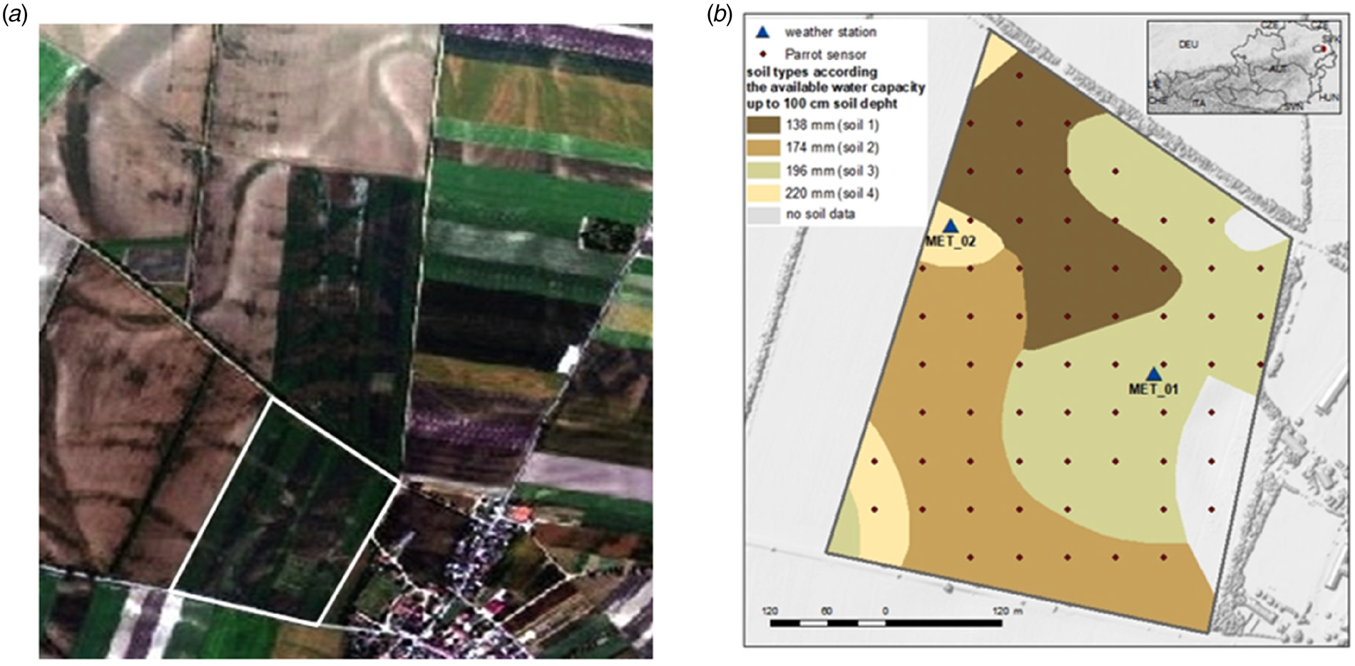
The experimental field is located in Rutzendorf (48°12′N, 16°33′E, 150 m asl) in the northeastern part of Austria (Fig. 1(b)). This region, called Marchfeld, is characterized by a Pannonian climate, a distinctive continental climate belonging to the temperate zone, with warm, partly hot and dry summers and cold winters with little snow (Thaler et al., Reference Thaler, Eitzinger, Trnka, Možný, Hahn, Wagner and Hlavinka2018). In the 17-ha experimental field, organic winter wheat was grown from 2018 to 2019 under rainfed conditions. The previous crop was grain peas. The sowing date was the 22 October 2018, the winter wheat was harvested on the 5 July 2019 and the yield was approximately 4600 kg/ha (mean value across the experimental field). The field was managed organically, and no fertilizer was used.
(a) Spatial representation of the soil surface colour (related to the sand content at the surface) and variability (Hymap, Marchfeld) within the field and test area (white framed) on 20/06/2006 (Eitzinger et al., Reference Eitzinger, Kersebaum and Formayer2009; project DROSMON). (b) In-situ measurement grid (50 × 50 m2) of Parrot sensors, the locations of the two weather stations and the soil classes of the water capacity of the soil layer 0–100 cm available for crops, derived from the eBod soil map, at the Rutzendorf test field (17 ha).

The soil type is chernozem, known for its highly variable A-horizon depth, which leads to significant local differences in the crop available water storage capacity, where the underlying C-horizon has a relatively high sand content with a relatively low available water storage capacity. The predominant spatial differences in soil texture at this trial site are shaped by the geomorphology of a terrace system with young river deposits of loess and by the former meandering of the Danube. This property leads to strong small-scale variation in the vertical soil texture characteristics in the upper soil layer of the main rooting depth of crops (up to approximately 1 m), especially with respect to the sand content, which is typical for the Marchfeld region (Brandtner, Reference Brandtner1954). The small-scale variability within the field is clearly recognizable in the Hymap image of the studied trial field, which presents the soil surface colours determined by the sand content at the surface (Fig. 1(a)).
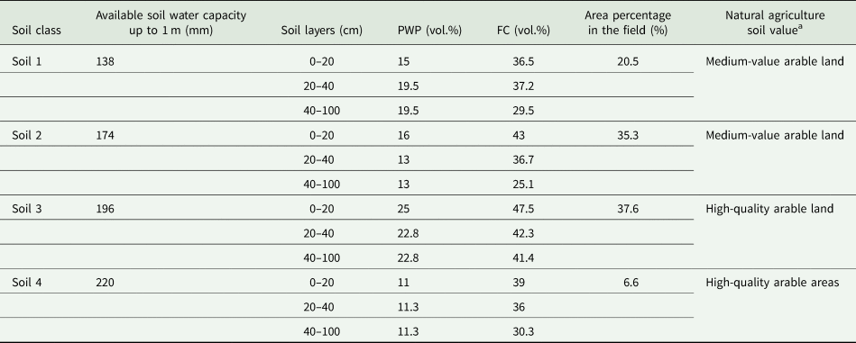
In accordance with the highest-quality soil map available from Austria ‘eBod’ (BFW, 2024), four different soil types with available water capacities (AWCs) ranging from 138 to 220 mm up to a 1 m soil depth, as defined by Murer (Reference Murer1998), are summarized in the test area (Fig. 1(b), Table 1).
Four soil classes according to the available water capacity (AWC), area percentage and natural agriculture soil value in the test field

PWP, permanent wilting point; FC, field capacity.
a According to eBod (www.bodenkarte.at).
In-situ SM measurements
In the first approach, a total of 65 grid points, sized 50 × 50 m2 (Fig. 1(b), Parrot sensor), were set up for permanent in-situ SM measurements at a 0–10 cm soil depth during the main winter wheat growing season from 4 April to 5 July 2019. Two SM sensors, namely, Parrot sensors, were placed at each grid point and averaged for the analysis. This allowed for obtaining a regular spatial distribution of SM in the topsoil. The Parrot sensors were developed by the wireless products manufacturer Parrot SA, Paris, France, and were designed for indoor and outdoor use to provide information on potted plants. In addition to the SM, the sensor provides the near-surface air temperature, light intensity and soil fertilizer content (Parrot, 2016). The water content of the soil is measured with a capacitive method, which requires calibration with respect to the physical properties of the soil (Xaver et al., Reference Xaver, Zappa, Rab, Pfeil, Vreugdenhil, Hemment and Dorigo2020).
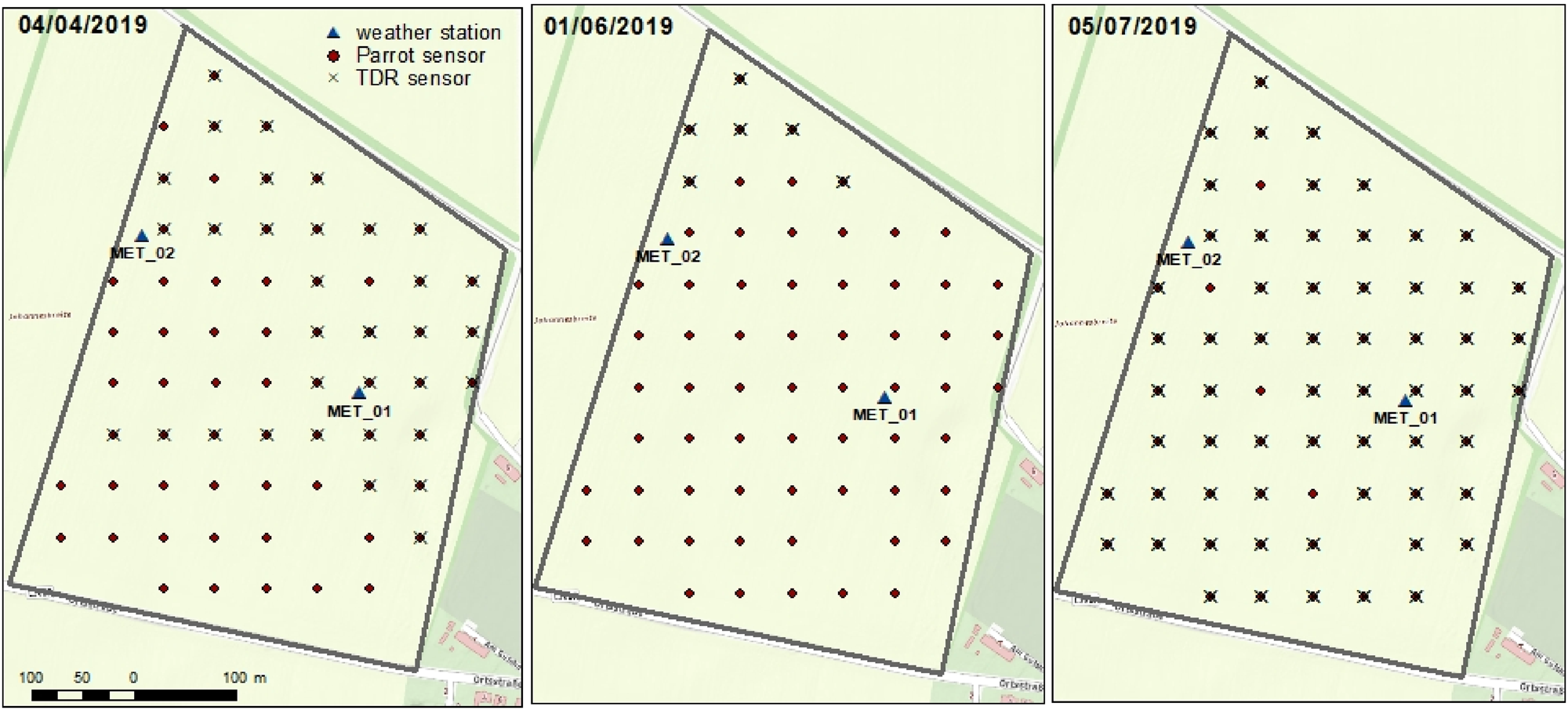
As reference samples and for calibration of the Parrot sensors, SM measurements representing a 0–10 cm soil depth, with a highly accurate handheld TDR sensor system (TRIME) (Topp et al., Reference Topp, Davis and Annan1980), were performed three times during the study period. All of these TDR measurements were conducted at locations where the Parrot sensors were installed, twice per location and averaged for calibration purposes (Fig. 2). The first reference data collection with the TDR sensor took place on 4 April 2019, and included 35 Parrot sensor locations within the experimental test site. Furthermore, TDR measurements of only seven Parrot sensor locations due to sensor failure were performed on 1 June 2019, and measurements of 59 Parrot sensor locations were performed on 5 July 2019.
In-situ measurement grid (50 × 50 m2) of Parrot sensors and grid points of the reference TDR sensor measurements on 04/04/2019, 01/06/2019 and 05/07/2019.

Two automated agrometeorological stations with various sensors were installed in the experimental field to collect time series data on continuous weather and soil conditions at a high-temporal resolution (10 min) (Fig. 1(b), weather station). The first weather station (Met_01) was located within the experimental field and conducted relevant micrometeorological measurements (air temperature, global radiation, relative air humidity and precipitation). In addition, three frequency-domain reflectometer (FDR) sensors (CS616, Campbell, Logan, USA) (Robinson et al., Reference Robinson, Campbell, Hopmans, Hornbuckle, Jones, Knight, Ogden, Selker and Wendroth2008) were placed vertically around the station, which presented the SM measured from a 0 to 30 cm soil depth (vol.%). The second agrometeorological weather station (Met_02) was situated at the western edge of the field and was equipped with the FDR method-based sensor ECH2O EC-5 (METER Group, Munich, Germany) (METER, 2024) in a soil profile representing the SM at 10, 20, 30, 40 and 50 cm soil depths (vol.%). Air temperature, global radiation, wind speed, relative air humidity and precipitation were also measured.
Remote-sensing-based SM estimates (S1ASCAT)
The second approach involved remote-sensing-based SM data, which were retrieved from Metop ASCAT and Sentinel-1 active microwave observations (S1ASCAT) using the Vienna University of Technology (TU Wien) change detection method (Wagner et al., Reference Wagner, Lemoine, Borgeaud and Rott1999a, Reference Wagner, Lemoine and Rott1999b; Naeimi et al., Reference Naeimi, Bartalis and Wagner2009). A new vegetation parameterization was incorporated into the retrieval algorithm for Metop ASCAT, according to a previous paper (Pfeil et al., Reference Pfeil, Vreugdenhil, Hahn, Wagner, Strauss and Blöschl2018). The SM estimates from Metop ASCAT, with an original sampling of 12.5 km, were disaggregated to 1000 m sampling using a temporal stability approach (Wagner et al., Reference Wagner, Pathe, Doubkova, Sabel, Bartsch, Hasenauer, Bloschl, Scipal, Martinez-Fernandez and Low2008; Hahn et al., Reference Hahn, Wagner, Steele-Dunne, Vreugdenhil and Melzer2021) based on 500 m Sentinel-1 backscatter observations. This data set is a precursor of the EUMETSAT Satellite Application Facility with the support of the Hydrology and Water Management (H SAF) disaggregated SM product H28, which was made available to the current study by TU Wien.
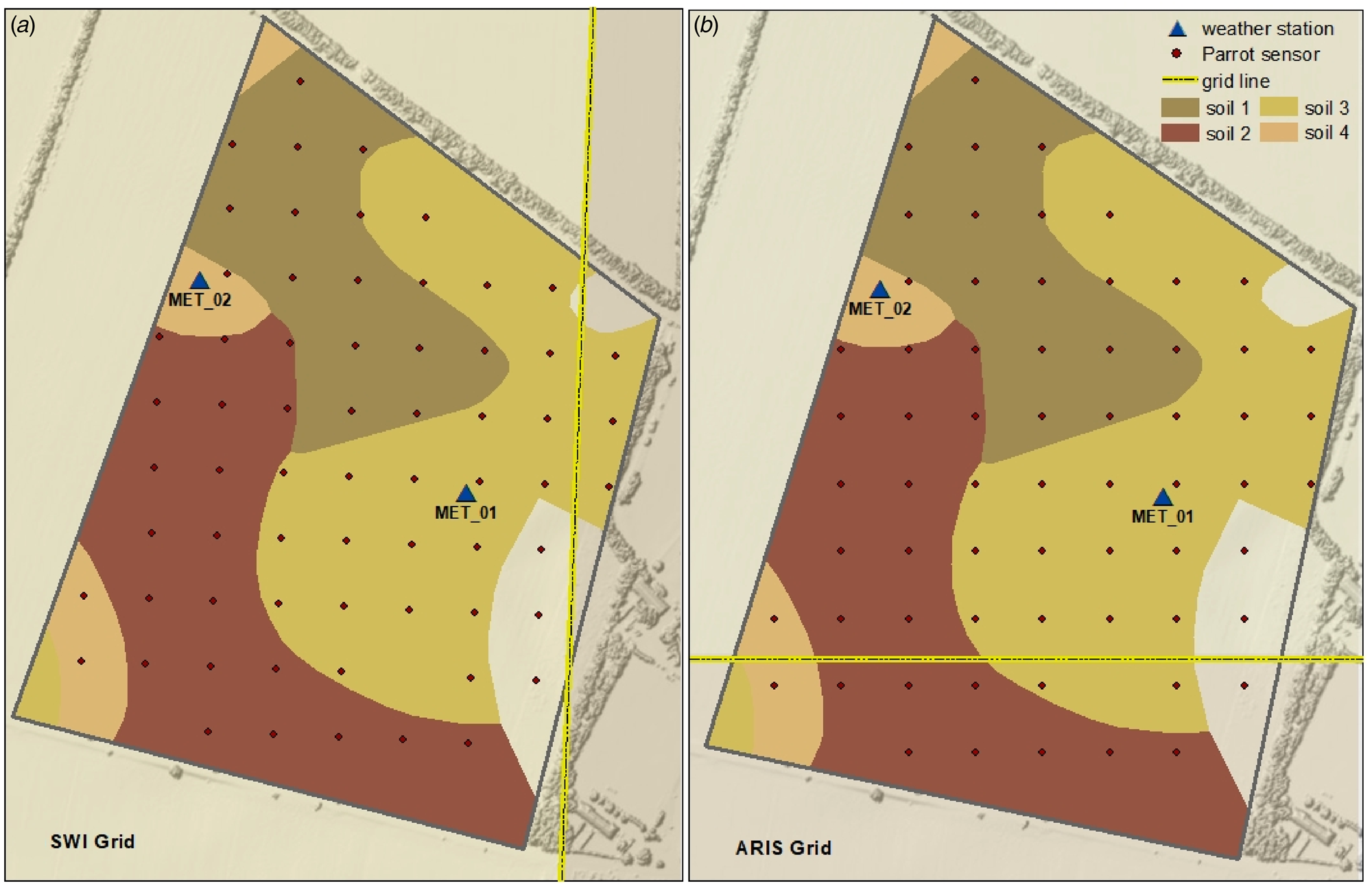
From the surface SM estimates, the soil–water index (SWI) was calculated. The SWI represents the SM profile at different soil depths as relative soil saturation (RSS), ranging from 0% SM at the permanent wilting point (PWP) to 100% SM at the FC (Brocca et al., Reference Brocca, Melone, Moramarco, Wagner and Hasenauer2010; Wagner et al., Reference Wagner, Hahn, Kidd, Melzer, Bartalis, Hasenauer, Figa-Saldaña, de Rosnay, Jann, Schneider, Komma, Kubu, Brugger, Aubrecht, Züger, Gangkofner, Kienberger, Brocca, Wang, Blöschl, Eitzinger, Steinnocher, Zeil and Rubel2013). The SWI was calculated using the exponential filter introduced in previous papers (Wagner et al., Reference Wagner, Lemoine, Borgeaud and Rott1999a, Reference Wagner, Lemoine and Rott1999b; Albergel et al., Reference Albergel, Rudiger, Pellarin, Calvet, Fritz, Froissard, Suquia, Petitpa, Piguet and Martin2008) with a characteristic time delay (T). The T value represents the smoothing of SM dynamics by infiltration, with higher T values corresponding to a higher degree of smoothing (Tong et al., Reference Tong, Parajka, Széles, Greimeister-Pfeil, Vreugdenhil, Komma, Valent and Blöschl2022) and representing increasing soil depths. SWI products are available daily on a 500 m grid, where the T values of 01 (SWI 01), 05 (SWI 05) and 10 (SWI 10) were used for analysis in the current study. The majority of the field was covered by only one S1ASCAT grid (Fig. 3(a)). The adjacent grid to the east contains only three Parrot measurement points and was therefore not included in the analyses because of the low number of measured values.
Grids overlapping with the field test site of 500 m: (a) remote-sensing-derived SM (SWI) and (b) ARIS model-simulated SM (RSS).

SM modelling
In the third approach, daily SM was modelled using the dynamic crop growth models DSSAT-CERES-Wheat (Hoogenboom et al., Reference Hoogenboom, Porter, Boote, Shelia, Wilkens, Singh, White, Asseng, Lizaso, Moreno, Pavan, Ogoshi, Hunt, Tsuji, Jones and Boote2019, Reference Hoogenboom, Porter, Shelia, Boote, Singh, White, Pavan, Oliveira, Moreno-Cadena, Lizaso, Asseng, Pequeno, Kimball, Alderman, Thorp, Jones, Cuadra, Vianna, Villalobos, Ferreira, Batchelor, Koo, Hunt and Jones2023; Jones et al., Reference Jones, Hoogenboom, Porter, Boote, Batchelor, Hunt, Wilkens, Singh, Gijsman and Ritchie2003) and AquaCrop (Steduto et al., Reference Steduto, Raes, Hsiao, Fereres, Heng, Izzi and Hoogeveen2008; Vanuytrecht et al., Reference Vanuytrecht, Raes, Steduto, Hsiao, Heng, Vila, Moreno and Moreno2014), as well as the GIS-based modelling system ARIS (Eitzinger et al., Reference Eitzinger, Daneu, Kubu, Thaler, Trnka, Schaumberger, Schneider and Tran2024).
The crop growth model DSSAT
The goal of the dynamic simulation model DSSAT-CERES is to comprehend the physiological mechanisms underlying plant growth at the daily simulation time step. A cultivar's growth and phenological development as a function of the photoperiod, thermal time and dry matter distribution can only be ascertained with crop-specific genetic coefficients (Babel et al., Reference Babel, Deb and Soni2019; Thaler et al., Reference Thaler, Berger, Eitzinger, Mahnaz, Shala-Mayrhofer, Zamini and Weihs2024). The functions of the initial accumulated biomass, the water and/or nitrogen stress coefficient and the actual leaf area index provide the dry biomass at a given stage (Deb et al., Reference Deb, Kiem, Babel, Chu and Chakma2015). The DSSAT model applies a soil water balance subroutine in which irrigation and precipitation are summed, and surface runoff, drainage, crop transpiration and soil evaporation are subtracted. Precipitation is provided by the daily weather data inputs, and irrigation is included via the experimental detail file and comprises the type of irrigation, the water supply efficiency and the date and amount of irrigation. Based on the soil conservation service (SCS) curve numbering approach (Ritchie, Reference Ritchie, Tsuji, Hoogenboom and Thornton1998), precipitation is split into infiltration and surface runoff. In the current study, the DSSAT version 4.8.2 was used. The input data for the model were weather, soil, genotype and management data. For this purpose, daily meteorological data from two weather stations (Met_01, Met_02) in the field were used: minimum and maximum temperatures (°C), solar radiation (MJ/m2) and precipitation (mm). Based on the eBod soil map (BFW, 2024), four different soil type classes (Fig. 1(b)) were derived for the trial field (Table 1) and used as model inputs. The classes were defined by the available water capacity of the 0–1 m soil layer (Murer et al., Reference Murer, Wagenhofer, Aigner and Pfeffer2004) (Table 1).
The crop growth model was calibrated for winter wheat (Thaler et al., Reference Thaler, Eitzinger, Trnka and Dubrovsky2012) and was based on the phenological components and grain yield. As the latter was only available for the entire field, the area-weighted simulated yield across all four soil types was used, with the weighting based on the proportion of area per soil class. The crop simulation was conducted from sowing on 22 October 2018 to maturity on 5 July 2019 without irrigation or fertilization.
The output of the model, which was used for the analysis, was the daily simulated SM (vol.%) of the two upper soil layers, 0–5 and 5–15 cm. As the in-situ measurements were conducted at a soil depth of 0–10 cm, the mean value of the two soil layers was additionally calculated to obtain a better approximation of the soil depth to the measured values (soil layer 0–10 cm).
The crop growth model AquaCrop
Like DSSAT, AquaCrop, which is based on the FAO approach (Allen et al., Reference Allen, Pereira, Raes and Smith1998), simulates growth processes such as biomass accumulation at daily time steps, with a focus on yield responses to water stress. As it is a generic crop model designed for irrigation planning, it uses a simplified crop growth scheme with respect to specific crop varieties or cultivar characteristics. Compared with other crop models, AquaCrop has a particular focus on water-related processes, which makes its soil module relatively detailed. It balances simplicity (to ensure usability) with a robust representation of processes such as water movement, salinity and soil fertility dynamics, all of which influence crop growth and yield. The model estimates plant growth by calculating the daily water balance, which includes inputs such as rainfall and irrigation and outputs such as evapotranspiration (ET) and runoff. AquaCrop uses normalized water productivity and the ratio of actual crop transpiration to reference ET to determine a crop's water-use efficiency (Steduto et al., Reference Steduto, Hsiao, Raes and Fereres2009). This information was then used to calculate the aboveground biomass. The yield is assumed to depend on the aboveground biomass and a reference harvest index, which is the ratio of the economic yield to the total aboveground biomass. Both the aboveground biomass and the harvest index must be calibrated for different crop types to ensure accurate yield predictions. This approach allows AquaCrop to simulate crop growth and yield under varying water availability and management practices (Steduto et al., Reference Steduto, Hsiao, Raes and Fereres2009; Vanuytrecht et al., Reference Vanuytrecht, Raes, Steduto, Hsiao, Heng, Vila, Moreno and Moreno2014; Babel et al., Reference Babel, Deb and Soni2019; Salman et al., Reference Salman, García-Vila, Fereres, Raes and Steduto2021).
The simulations were conducted using AquaCrop version 7.1. Weather, soil, crop and management data are required as input data. In addition to the daily weather data used for DSSAT (minimum and maximum temperature [°C], solar radiation [MJ/m2] and precipitation [mm]), the grass reference ET for AquaCrop was included. The soil and management data were identical to those used for DSSAT; winter wheat was calibrated using the phenology and yield data (Thaler et al., Reference Thaler, Gobin and Eitzinger2017).
As an output, AquaCrop also has the daily simulated SM (vol.%) of the two upper soil layers 0–5 and 5–15 cm. Furthermore, the 0–10 cm layer was determined with the mean value of the abovementioned layers.
Agricultural risk information system
The ARIS model was developed as a monitoring and forecasting tool for agricultural risk in Austria and operates at a daily time step (Eitzinger et al., Reference Eitzinger, Daneu, Kubu, Thaler, Trnka, Schaumberger, Schneider and Tran2024). Compared with AquaCrop, it uses the FAO soil‒crop water approach (Allen et al., Reference Allen, Pereira, Raes and Smith1998) with a simplified calculation scheme, which is based on SoilClim (Hlavinka et al., Reference Hlavinka, Trnka, Balek, Semerádová, Hayes, Svoboda, Eitzinger, Možný, Fischer, Hunt and Žalud2011). The soil‒crop water module calculates daily soil‒crop water balance parameters at a 500 m grid scale across Austria within a GIS scheme, including soil water depletion, related drought and heat stress impacts on crop yield and other abiotic and biotic cropping risks.
The model uses the spatial input data of various parameters such as 1 km grid-based weather data (INCA), the available soil water capacity for two predefined soil layers up to 1 m soil depth as a 0.5 km grid based on the eBod soil map (PWP, FC) (BFW, 2024), the CORINE Land Cover and a digital elevation model. Thus, for the purpose of calculating the soil crop water status and crop water demand, the ARIS simulation considers the local soil and weather conditions in addition to the phenological development of the chosen crop type (Eitzinger et al., Reference Eitzinger, Daneu, Kubu, Thaler, Trnka, Schaumberger, Schneider and Tran2024).
For the current study, the daily 500 m output grid ‘RSS ’ (%) was used for the test field at soil depths of 0–10 cm (RSS 0–10), 0–20 cm (RSS 0–20) and 0–40 cm (RSS 0–40) under winter wheat conditions for the analysis. Like SWI, RSS ranges from 0% SM at the PWP to 100% SM at the FC. As the values between the two grids on the field hardly differed (mean difference between 0–10 and 0–20 cm = 0.004%, and 0–40 cm = 0.007%), the values of the larger merged grid of 500 m size were used for the analysis (Fig. 3(b)).
Data compilation
High-resolution SM measurements
Based on a comparison of the two sensor types, TDR and Parrot, the Parrot sensors were calibrated with the help of a polynomial regression and subsequently validated with the measured values from the two weather stations.
Ordinary kriging was used in ArcGIS to display the spatial distribution of the Parrot point values. This geostatistical approach is widely used to generate unbiased estimates of regionalized variables in specific areas (Bayraktar and Turalioglu, Reference Bayraktar and Turalioglu2005; Emery, Reference Emery2005; Balasundra et al., Reference Balasundra, Husni and Ahmed2007). Ordinary kriging calculates the mean value of the variable value at a specific point (Kumar et al., Reference Kumar, Rao, Burman, Kumar and Samui2023). It relies on input data points, their positions and spatial variation information derived from a variogram or covariance equation. These requirements are generally met effectively, even under less-than-ideal conditions (Webster and Oliver, Reference Webster, Oliver, Webster and Oliver2007). In the current study, 65 measurements at 50 × 50 m2 spacing provided a sufficient sample size and spatial distribution for generating a reliable variogram and achieving accurate spatial interpolation. The method's ability to minimize error variance further ensures precise and unbiased predictions (Kumar et al., Reference Kumar, Rao, Burman, Kumar and Samui2023).
Remote-sensing estimates and crop model simulations of SM
In a further step, the SM values estimated from remote-sensing (SWI), crop (vol.%) and ARIS (RSS) models were compared with the in-situ measurements and statistically evaluated. Since four soil types were simulated in the crop growth models AquaCrop and DSSAT, a spatial comparison was also possible. The simulated results were compared with the average Parrot measurements per soil type. For three Parrot measurement points (Fig. 1(b)), no soil data were available; they were omitted from the analysis.
For the SWI and RSS data, only one SM value was used for the entire test field because of the underlying grid size (Fig. 3); thus, only the temporal dynamics could be compared. For a statistical comparison between the different SM estimated values and the measurements of the Parrot sensors, the mean values of all the Parrot sensors within the two grids were calculated. Additionally, for the AquaCrop and DSSAT crop growth models, the area-weighted SM value (in vol.%) of the four soil classes was calculated to obtain one daily value per model for the whole test field.
Although the in-situ measurements and AquaCrop and DSSAT simulations specify and analyse SM in vol.%, the data for the ARIS (RSS) and remote-sensing-based SM values (SWI) are reported as a relationship with soil saturation (%). The standard score (z) was applied for standardization to compare the Parrot and output values with those of the RSS and SWI units:

where x is the raw score or observed value, μ is the mean and σ is the standard deviation.
Statistical analysis
Various statistical indicators listed below were used to compare, validate and evaluate the modelled (DSSAT, AquaCrop, and ARIS) and estimated (SWI) SM data with the measured data (Parrot).
Mean bias error (MBE): Without considering the direction of the differences, the MBE calculates the average difference between the simulated and observed values. A maximum score of 0 denotes that the simulated model is free of bias. The MBE is reported in the same units. A positive MBE indicates that the simulated values are, on average, higher than the observed values, whereas a negative MBE indicates the opposite (Janssen and Heuberger, Reference Janssen and Heuberger1995). The equation for MBE is as follows:

where n is the number of observations, Pi is the predicted value for the i-th observation and Oi is the observed value for the i-th observation.
Mean absolute error (MAE): The average of all absolute errors, presented in the same units, is known as the MAE (Willmott and Matsuura, Reference Willmott and Matsuura2005). The equation for the MAE is as follows:

where n is the number of observations, Pi is the predicted value for the i-th observation and Oi is the observed value for the i-th observation.
Root mean square error (RMSE) and unbiased RMSE (ubRMSE): RMSE is a widely used metric for assessing the accuracy of a model's predictions. It measures the average magnitude of the errors between the predicted values and observed values (Hyndman and Koehler, Reference Hyndman and Koehler2006). The equation for the RMSE is as follows:

where n is the number of observations, Pi is the predicted value for the i-th observation and Oi is the observed value for the i-th observation.
An alternative to the RMSE that accounts for prediction bias is the ubRMSE. It is particularly useful when the mean of the observed values is significantly different from the mean of the predicted values. The ubRMSE is calculated by removing the mean of the observed values from the predictions before computing the RMSE, which helps to provide a more accurate measure of the model's performance without the influence of systematic bias (Entekhabi et al., Reference Entekhabi, Reichle, Koster and Crow2010). The equation for ubRMSE is as follows:

where n is the number of observations, Pi is the predicted value for the i-th observation, Oi is the observed value for the i-th observation, $\bar{P}$ is the mean of the predicted values and $\bar{O}$
 is the mean of the observed values. A better model performance for both indicators is represented by a smaller value.
Kling–Gupta efficiency (KGE): The goodness-of-fit measure developed by Gupta (Gupta et al., Reference Gupta, Kling, Yilmaz and Martinez2009) provides a diagnostic breakdown of the Nash–Sutcliffe efficiency, making it easier to analyse the relative significance of its various components (correlation, bias and variability) in the context of hydrological modelling. The index was revised twice: once to guarantee that the bias and variability ratios are not cross-correlated (Kling et al., Reference Kling, Fuchs and Paulin2012) and once to prevent anomalously negative KGE values or values when the mean is near zero (Tang et al., Reference Tang, Clark and Papalexiou2021). The range of KGE is from −∞ to 1, and the closer two sets of simulated and observed data are to 1, the more similar they are. The KGE formulation is as follows:

where r is the linear correlation coefficient between the observed and predicted values, γ is the ratio of the coefficient of variation of the predicted values to the coefficient of variation of the observed values and β is the ratio of the mean of the predicted values to the mean of the observed values.
The components are defined as follows:


where cov(P, O) is the covariance between the predicted (P) and observed (O) values, σ P is the standard deviation of the predicted values, σ O is the standard deviation of the observed values, $\bar{P}$ is the mean of the predicted values and $\bar{O}$
 is the mean of the observed values.
Coefficient of determination (R 2) and adjusted coefficient of determination (adj-R 2): The percentage of the variation in the dependent variable that can be predicted from the independent variable(s) is known as the coefficient of determination (Draper and Smith, Reference Draper, Smith, Draper and Smith1998). The equation for R 2 is as follows:

where n is the number of observations, Oi is the observed value for the i-th observation, Pi is the predicted value for the i-th observation and $\bar{O}$ is the mean of the observed values.
Although R 2 assumes that each variable explains the variation in the dependent variable, adj-R 2 represents the percentage of variation explained by only the independent variables that actually affect the dependent variable (Raju et al., Reference Raju, Bilgic, Edwards and Fleer1997):

where R 2 is the coefficient of determination, n is the number of observations and k is the number of predictors (independent variables) in the model.
Results
Calibration of the Parrot sensors
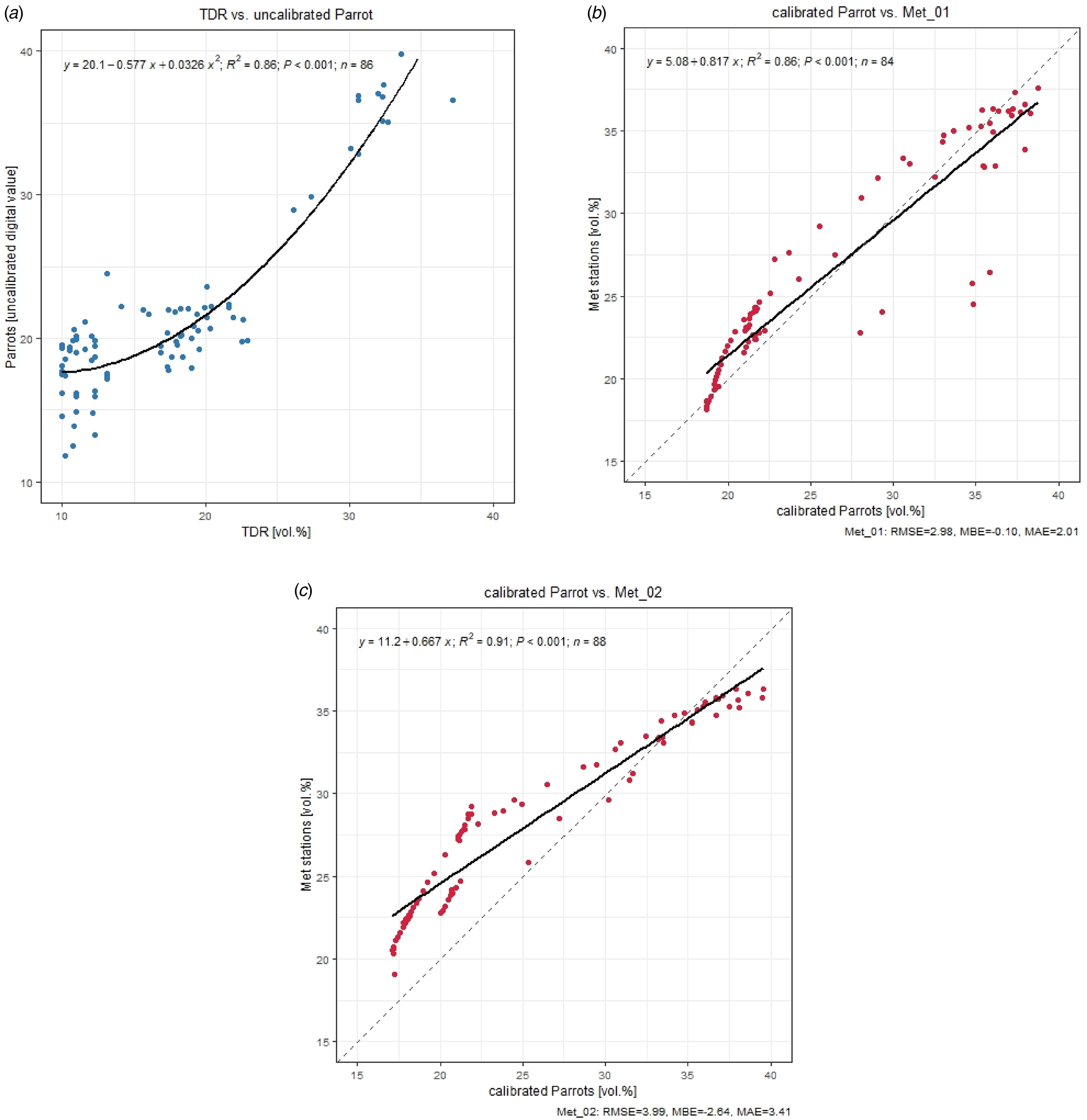
With the help of polynomial regression (Fig. 4(a)), the SM content from the Parrot measurements was calibrated with TDR values (R 2 = 0.86):

(a) Polynomial regression of SM TDR (vol.%) v. uncalibrated Parrot sensors (0–10 cm soil depth), including R 2 (coefficient of determination); (b) linear regression of SM (vol.%) calibrated Parrot sensors (0–10 cm soil depth) v. weather station Met_01 (0–30 cm soil depth), including R 2, RMSE, MBE and MAE. The dashed line represents the 1:1 line; (c) linear regression of SM (vol.%) calibrated Parrot sensors (0–10 cm soil depth) v. weather station Met_02 (0–20 cm soil depth), including R 2, RMSE, MBE and MAE. The dashed line represents the 1:1 line.

Following calibration, the Parrot values were compared with the data obtained from the two weather stations (Fig. 4(b)). The closest locations of the Parrot measurements from the two weather stations were used. Located in the field centre (Fig. 1(b)), the Met_01 station represents the SM measurement of the 0–30 cm soil depth. With an MBE of −0.1, an RMSE of 2.97 vol.%, an MAE of 2.01 vol.% and an R 2 of 0.86, the agreement was very high. The SM measurements at Met_02 represent a measurement at the 10 cm soil depth (horizontally suited sensor), which can be regarded as an approximated mean value for the 0–20 cm soil depth. The agreement reflects the result of Met_01 and was also very high, with an R 2 of 0.91, an RMSE of 3.99 vol.%, an MBE of −2.64 and an MAE of 3.41 vol.%.
Spatial variability
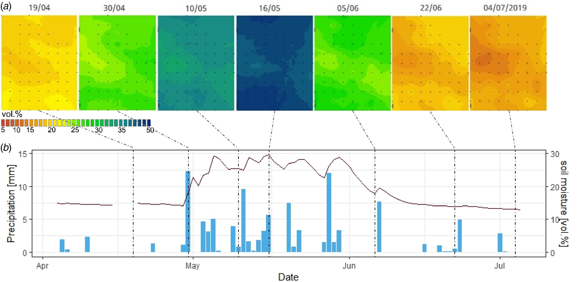
In Fig. 5(a), seven selected days with different levels of SM during the wheat growing season of 2019 are displayed, reflecting the seasonal precipitation pattern. At the beginning of the measurement campaign (04/2019), dry soil conditions prevailed in the field and hardly any precipitation occurred in April (Fig. 5(b)). In contrast, the entire month of May experienced intensive precipitation, which led to higher soil water contents. Individual rainfall events occurred in June, but the SM content decreased towards the end of the measurement campaign again because of the high crop water demand of a fully developed active canopy. The SM content at the study site for the entire time series can be found in Appendix 1.
(a) Spatial variability of SM (vol.%) across the experimental field at Rutzendorf on 19/04, 30/04, 10/05, 16/05, 05/06, 22/06 and 04/07/2019, as determined by kriging. The dots represent the in-situ Parrot measurement points. (b) Daily precipitation (mm, bars) and mean SM content (vol.%, line) determined by Parrot measurements at the experimental field in Rutzendorf from 04/04 to 05/07/2019; the dotted lines represent the days of the SM map shown above.

The temporal changes in the interpolated SM grid reflect the spatial soil type distribution according to the soil map relatively well, showing that the areas with the lowest SM level (corresponding to a low soil water holding capacity due to the same crop surface conditions) often remain drier in all phases of SM, except for near the extreme levels (e.g. near the PWP and FC). Slightly changing patterns throughout the season are caused by the interaction of soil water and nutrient storage capacity with biomass development, which in turn affect the crop transpiration rate and soil water uptake.
Time series of different SM products
SM contents of the different soil types from the crop growth models
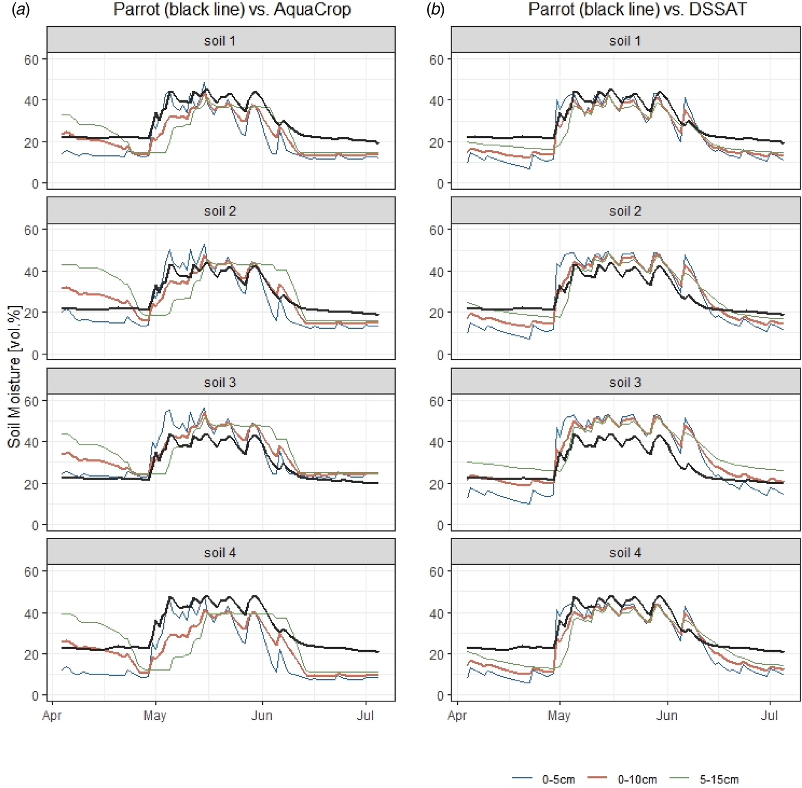
While the SM values from AquaCrop in soils 1 and 2 agree quite well with the Parrot measurements, those in soils 3 and 4 clearly overestimate and underestimate, respectively, the modelled SM (Fig. 6). This finding is also partly reflected in the DSSAT results, where soils 1, 2 and 4 show good agreement and soil 3 clearly overestimates. Additionally, the SM in AquaCrop at 5–15 cm is smoother and has a time lag in comparison to that in the top layer. In regard to DSSAT, this difference is less noticeable. Using the average values (0–10 cm), the simulated values could be approximated to the measured values, especially for DSSAT.
SM (vol.%) time series from the Parrot sensors (black line) v. (a) AquaCrop and (b) DSSAT (soil depth 0–5 cm blue line, 0–10 cm red line, 5–15 cm green line) according to the four soil types during the wheat spring growing season in 2019.

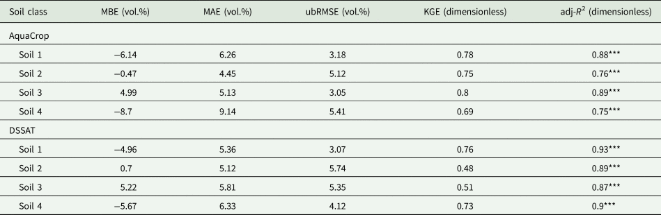
When looking at the MBE for both models at a soil depth of 0–10 cm, soils 1 and 4 have the greatest negative deviations (Table 2). Soil 3 clearly overestimates with an MBE of 5 vol.%. Soil 2 exhibits a positive MBE in DSSAT, but it is underestimated in AquaCrop. The MAE varies from 4 to 6 vol.% for the first three soil classes; however, it is significantly higher for soil 4, especially for AquaCrop. The ubRMSE values are the lowest for soils 1 and 3 in AquaCrop, as well as for soils 1 and 4 in DSSAT, with values <4.2 vol.%. These soils also have the highest KGE values (>0.72), indicating greater similarity between the simulated and observed data. With an adj-R 2 exceeding 0.87 for DSSAT and 0.75 for AquaCrop, the model fit was strong.
Statistical analyses of Parrot-measured SM v. SM simulated by AquaCrop at 0–10 cm and DSSAT at 0–10 cm soil depth according to the four soil classes

MBE, mean bias error; MAE, mean absolute error; ubRMSE, unbiased root mean square error; KGE, Kling–Gupta efficiency; adj-R 2, adjusted coefficient of determination.
Signif. codes: P-value <0.001 ‘***’ (highly significant); 0.001 ⩽ P-value <0.01 ‘**’ (very significant); 0.01 ⩽ P-value <0.05 ‘*’ (significant); P-value ⩾0.05 ‘ ’ (not significant).
One grid-point remote sensing and crop model SM estimates v. Parrot-measured SM
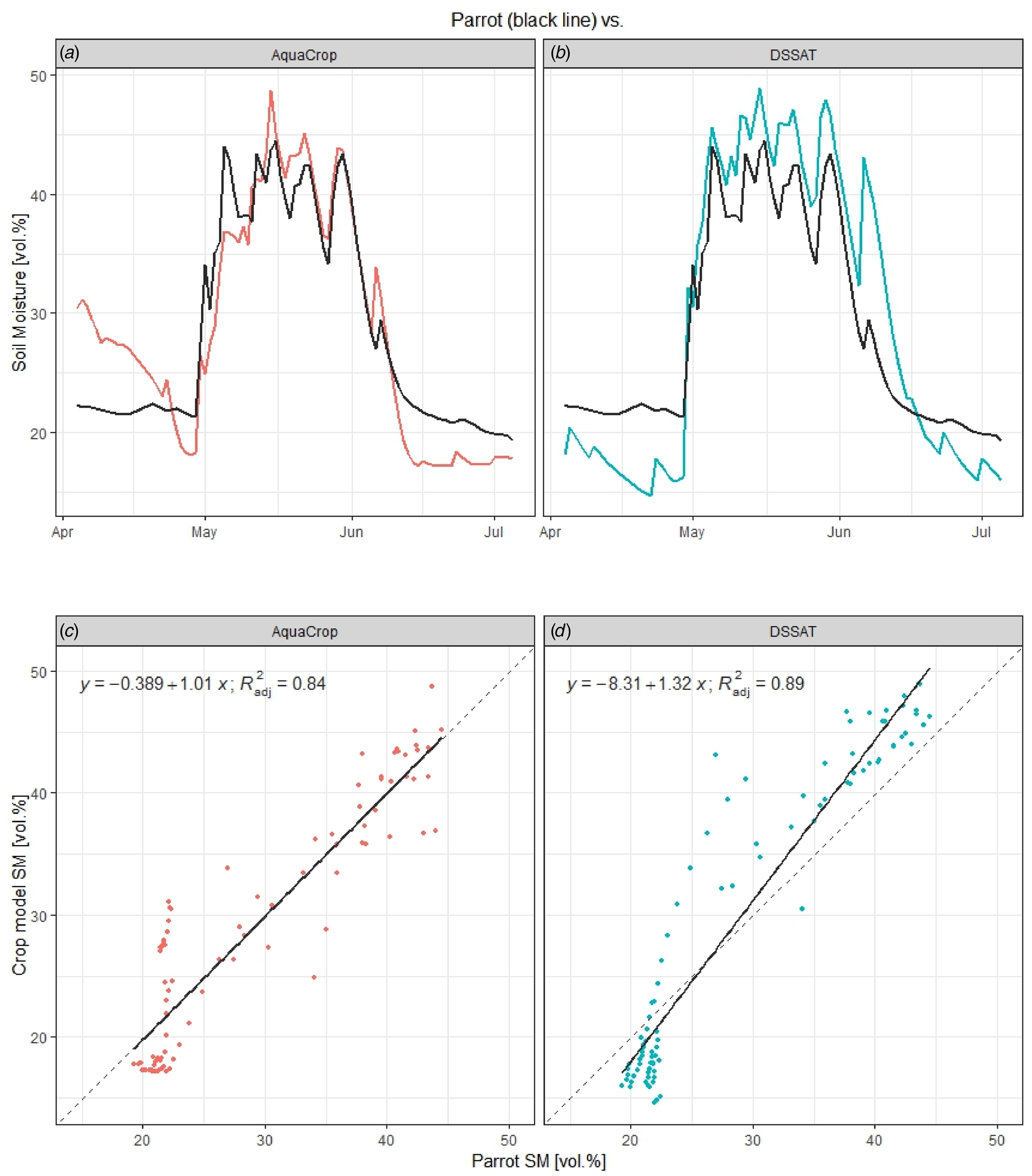
The time series and regression analysis between the measured and simulated SM (0–10 cm) using the DSSAT and AquaCrop models are shown in Fig. 7.
SM (vol.%) time series from the Parrot sensors (black line) v. (a) AquaCrop (red line) and (b) DSSAT (blue line) (soil depth 0–10 cm) during the wheat spring growing season in 2019 (average value over the experimental field); linear regression and R 2 of SM (vol.%) Parrot v. (c) AquaCrop and (d) DSSAT; the dashed line represents the 1:1 line.

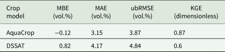
Both simulations closely correspond to the measured values (Fig. 7(a)). In AquaCrop, the simulated SM starts much higher (30.5 vol.% compared with 23 vol.% for Parrot) and then decreases to the same level as the Parrot measurements. At the beginning of May, however, the increase in SM shifts slightly and starts approximately 2 days later. A lower SM is simulated at the end of the measurement period. The adj-R 2 value of 0.84 is high (Fig. 7(b)). For the AquaCrop model, an ubRMSE of 3.87 vol.%, an MBE of −0.12 vol.%, an MAE of 3.15 vol.% and a KGE of 0.87 indicate very good performance (Table 3).
Statistical analyses of Parrot-measured SM (averaged over the field) v. SM simulated by AquaCrop at 0–10 cm and DSSAT at 0–10 cm soil depth (area-weighted over the field)

MBE, mean bias error; MAE, mean absolute error; ubRMSE, unbiased root mean square error; KGE, Kling–Gupta efficiency.
Starting in April, the DSSAT displays a noticeably lower SM. By the beginning of May, it rises to 45 vol.% and reaches the same value as the Parrot measurements. The simulations in May exhibit the same curve and peaks as the measured values, but they are 2–3 vol.% overestimated. The simulated SM decreases later and reaches a lower value than the measured SM at the end of the measurement period. The adj-R 2 of 0.89 is slightly higher than that for AquaCrop (Fig. 7(b)). The simulations overestimate the SM slightly (MBE = 0.82 vol.%), the MAE is 4.17 vol.%, the ubRMSE is 4.84 vol.% and the KGE is 0.6, which indicates good performance but is slightly poorer than that of AquaCrop (Table 3).
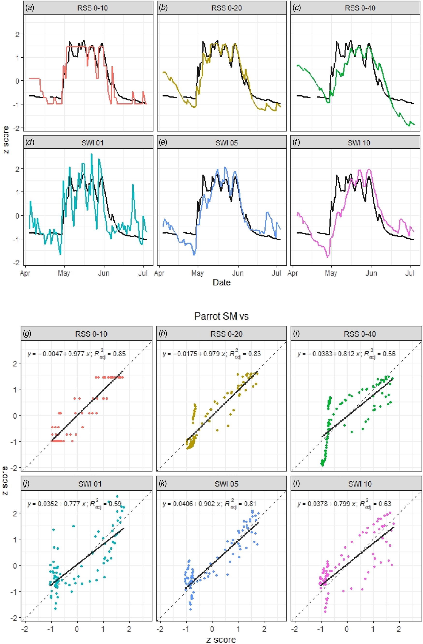
The Parrot SM measurements with the three different RSS (ARIS model) and SWI (S1ASCAT) SM values were compared by applying mean-standard scaling (z score), and the (a) time series and (b) regression analysis are presented in Fig. 8.
SM time series from the Parrot sensors (black line) v. ARIS model-simulated SM (a) RSS 0–10 (soil depth 0–10 cm), (b) RSS 0–20 (soil depth 0–20 cm), (c) RSS 0–40 (soil depth 0–40 cm) and remote-sensing-derived SM (soil–water index) (d) SWI 01 (time delay 1), (e) SWI 05 (time delay 5) and (f) SWI 10 (time delay 10); linear regression and R 2 of Parrot v. (g) RSS 0–10, (h) RSS 0–20, (i) RSS 0–40, (j) SWI 01, (k) SWI 05 and (l) SWI 10; the dashed line represents the 1:1 line (SM values are converted into standard scores).

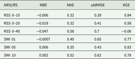
The Parrot measurements start in April with very dry SM values, which have a standard deviation of 0.8 that is below the mean value. On the other hand, the ARIS shows higher values at all three different soil depths. From the beginning of May, the SM increases significantly, with the RSS showing good agreement with the Parrot measurements. RSS 0–20, in particular, indicates very good correspondence up to the end of the measurement period. While the soil depth of 0–10 cm displays biased fluctuations, RSS 0–40 shows a shift in the SM values because it represents a deeper soil layer than the Parrot measurements with higher ‘memory’. In May, for example, the z score of RSS 0–40 increases with a delay of up to 15 days to the same value as that of Parrot, and at the end of the measurement period, it is clearly below the Parrot values. The adj-R 2 is strong, with 0.85 for RSS 0–10, 0.83 for RSS 0–20 and 0.56 for RSS 0–40. All three simulations show an underestimation, which is most pronounced for RSS 0–40 (MBE = −0.05). The ubRMSE of 0.4 and the MAE of 0.32 for RSS 0–10 as well as RSS 0–20 are the lowest values. Greater deviations are observed at RSS 0–40, with an ubRMSE of 0.7 and an MAE of 0.58 (Table 4).
Statistical analyses of the Parrot-measured SM v. ARIS model-simulated SM RSS 0–10 (soil depth 0–10 cm), RSS 0–20 (soil depth 0–20 cm), RSS 0–40 (soil depth 0–40 cm) and remote-sensing-derived SM (soil–water index) SWI 01 (time delay 1), SWI 05 (time delay 5), and SWI 10 (time delay 10); SM values are converted into standard scores (dimensionless)

MBE, mean bias error; MAE, mean absolute error; ubRMSE, unbiased root mean square error; KGE, Kling–Gupta efficiency.
ARIS model-simulated soil moisture: RSS, relative soil saturation; RS (remote-sensing)-derived soil moisture; SWI, soil–water index.
The SWI derived from S1ASCAT data shows the best agreement at SWI 05, with an adj-R 2 of 81% (similar to ARIS RSS 0–20), and the time series is highly consistent with the Parrot values, except for some temporal overestimations. While SWI 01 has very strong fluctuations compared with the Parrot values, SWI 10 is characterized by a delay in the SM peak in May, similar to RSS 0–40, because it represents a deeper soil layer and the applied algorithm. Nevertheless, the adj-R 2 values of 59% for SWI 01 and 63% for SWI 10 are good; the temporal course, compared with the Parrot values, fits well. The ubRMSE is slightly higher for RSSs between 0.4 and 0.6, the estimated SMs are for SWI 05 and SWI 10 overestimated (positive MBE) and the MAEs are between 0.35 and 0.52 (Table 4).
Discussion
Accurate estimates of soil water availability, for example, are crucial for assessing drought impacts and mitigating yield loss. The interface between soil and climate determines the agricultural production potential, and understanding the SM regime is essential for identifying cropping risks and optimizing yields. However, high-resolution spatial‒temporal data collection is expensive and time-consuming because of the lack of modern in-situ SM networks. As an application case in the current study, a set of actual best available databases (gridded soil map and weather data sets), modelling tools and remote-sensing methods under practical conditions at a field test site in an Austrian arable region were considered. In that context, the performance of selected spatial‒temporal SM estimation methods at the field scale was revealed, showing that the use of all three methods together could provide added value by checking data for errors or reliability, using them for gap filling or extending limited time series. For example, the study by Weir and Dahlhaus (Reference Weir and Dahlhaus2023) emphasized the lack of a continuous, accurate method for determining SM contents at the field level, which is a particular challenge for extensive dryland farming systems. Thus, combining different approaches, e.g. integrating remote-sensing data into crop growth models (e.g. Ines et al., Reference Ines, Das, Hansen and Njoku2013; Mishra et al., Reference Mishra, Cruise and Mecikalski2021; Zhou et al., Reference Zhou, Geng, Yang, Hu, Sheng and Lou2022) or calculating different approaches and using them as an ensemble, is possible. As a result, the accuracy, robustness and flexibility of SM estimates can be improved.
Using a 65-point measurement grid (0–10 cm soil depth) in the current study, it was possible to obtain an SM value in a 50 m grid on a 17-ha winter wheat test field. This approach allowed the spatial and temporal SM dynamics for the weather conditions of the year of investigation (2019) to be visualized. Within the test field, different near-surface (0–10 cm) SM levels were observed at any time during the growing season, which depended on the spatial variation in soil conditions but also likely changed to some extent in the interaction with the spatial variation in crop biomass development and associated crop water uptake (these variations were observed but not measured). Soil properties such as the pore volume, soil texture, organic content and soil structure affect the amount and length of time the soil can store water and make nutrients available for crops and consequently define the entire growth process, as well as the related SM regime (Huang et al., Reference Huang, Hartemink and Kucharik2021). Consequently, as expected, within the test field, the areas with the lowest SM content (corresponding to a low soil water holding capacity) remained frequently drier in all phases of SM, with the exception of areas near the extreme levels (e.g. near the PWP and FC). These drier areas were also more affected by drought stress and presented a lower crop biomass. Despite the interactions with biomass and related crop water use, the temporal changes in the interpolated near-surface (0–10 cm) SM grid still reflect the spatial soil type distribution according to the soil map fairly well, although the soil map is related to deeper soil layers, adding some further uncertainty.
Using the AquaCrop and DSSAT crop growth models, SM was determined based on four soil classes and was thus the only approach that was also able to show spatial variability within the field. Both models exhibit similar responses to those of the measurements, with underestimations of the topsoil layer SM during dry phases and overestimations during wet phases. The 0–5 cm soil layer water content shows high sensitivity to evaporation and transpiration resulting in strong daily fluctuations in measurements as well as simulated by DSSAT and AquaCrop. The Parrot sensor measurements, however, do not show such strong peaks. The 5–15 cm soil layer, which is already part of the main rooting zone, has significant impact on crop water availability, which limits crop growth during drought periods without irrigation. The best agreement between the measured and modelled SM was achieved with AquaCrop in soils 1 and 3 (KGE ⩾ 0.78; adj-R 2 ⩾ 0.88) and with DSSAT in soils 1 and 4 (KGE ⩾ 0.73; adj-R 2 ⩾ 0.9). However, the Austrian soil map (eBod) (BFW, 2024) may have potential bias at different spatial resolutions. Even when attempting to include different soil types in the modelling tasks for the two crop models, it did not succeed in representing small-scale differences in soil conditions. Although a very sophisticated product, the Austrian soil map still has too coarse a spatial resolution for resolving within-field-scale soil property variations necessary for high-efficiency precision farming applications such as fertilization or irrigation. Furthermore, the in-situ measured data represent only the SM at the 0–10 cm soil depth, where additional soil cultivation effects might reduce the soil water holding capacity. These temporal (seasonal) changes in the soil pore size distribution and related changes in the soil water holding capacity are not represented in the soil map or in the crop models.
The average Parrot SM values over the whole test field were compared with the 500 m grid SM values of the ARIS model, the remote-sensing-based S1ASCAT-SWI product and the average SM values simulated by AquaCrop and DSSAT. This approach can be used to determine which SM estimation methods are suitable for quantifying temporal SM dynamics at a resolution of 500 m. Based on the results of the statistical analysis, the data are a valuable and objective source for estimating SM in a grid of 500 m. In particular, the RSS 0–10, RSS 0–20, SWI 05, AquaCrop and DSSAT 0–10 cm are the most robust indicators of SM for the topsoil (adj-R 2 ⩾ 81%). Nevertheless, the SM estimates of SWI 01 and SWI 10 also provide valid and useful SM estimates at high-temporal resolutions. The spatial and temporal resolutions of the S1ASCAT-SWI products are related to the spatial resolution of the ASCAT sensor, the assumptions of the SM algorithm and the disaggregation scheme, which together determine the final resolution of the SM product. If deeper soil layers are considered, as with RSS 0–40 or SWI 10, a shift and bias in SM can be clearly recognized. These attributes can also be observed in the two models in the 5–15 cm soil layer and are particularly pronounced in AquaCrop.
A comparison of the two crop growth models reveals that DSSAT exhibits slightly higher deviations to measured SM values than AquaCrop across the entire study area. Although AquaCrop underestimates the topsoil layer water content at the beginning of the study period, DSSAT shows higher values especially in May. This can be attributed to differences in the calculation of root expansion and related root water extraction over the vertical soil profile, which was not calibrated for the models in this study.
Research has shown that the direct top-down, high-spatial resolution detection of the spatial variability of SM below a ‘crop field’ scale in the range of a few metres is currently not possible with the investigated methods S1ASCAT-SWI, large-area soil map-based crop models (AquaCrop and DSSAT) and GIS-based (ARIS) simulations. However, in field-based precision farming applications, several methods, such as mechanized soil probing; soil surface type estimations by an RGB analysis; high-spatial resolution leaf nitrogen content; sophisticated, ground-calibrated satellite products; GPS-referenced yield estimates; data-driven approaches and others (e.g. Mani et al., Reference Mani, Mandal, Biswas, Sarkar, Mitran, Meena, Mitran, Meena and Chakraborty2020; Rayhan Shaheb et al., Reference Rayhan Shaheb, Sarker, Shearer, Michael and Indi2022; Rozenstein et al., Reference Rozenstein, Cohen, Alchanatis, Behrendt, Bonfil, Eshel, Harari, Harris, Klapp, Laor, Linker, Paz-Kagan, Peets, Rutter, Salzer and Lowenberg-DeBoer2023), are available to resolve spatial soil variations at a very high resolution of a few metres. The combined use of different data sources and applications may further foster the development of high-spatial data sets applicable for a wide set of applications.
Nevertheless, the analysis presents a good temporal correlation at the 17-ha field-level mean SM estimates between the in-situ sensors, the S1ASCAT satellite remote-sensing product and the crop model simulation results. Thus, both methods can estimate the field-level SM temporal variation quite well, which is an important step forward in determining SM stress thresholds for crop production and is therefore an important tool for increasing the resilience and resource efficiency of cropping systems through adaptation measures, at least at the regional planning level. However, high-spatial resolution in-situ sensors and remote sensing (e.g. by drones or new satellite products) for increasing either the spatial resolution of derived soil properties or direct near surface moisture will have considerable application potential for precision or smart farming techniques in the next decades.
Conclusions
In the current study, three different approaches to determine the high-resolution SM content in a winter wheat field in northeastern Austria were determined and compared: in-situ measurements, remote-sensing data and model-based SM estimates. The spatial variability in the field represented by the in-situ measurements cannot be captured by the use of currently available national, sophisticated soil maps with the same spatial variation precision as the methods investigated. Even if different soil types can be used as inputs in crop models, the soil map base data are currently not accurate enough at such a spatial resolution, as shown in the current case. Nonetheless, the analysis reveals a good temporal correlation at the mean SM level. Thus, different methods can be used to assess the temporal variation in SM contents at the field level quite well. This tool is crucial for determining the thresholds for SM stress in crop production to increase the resilience and resource efficiency of cropping systems through adaptation measures at the regional level.
Supplementary material
The supplementary material for this article can be found at https://doi.org/10.1017/S0021859625000036
Acknowledgements
This work was supported by the BMon project (project no. 872408, ASAP 14) funded by FFG, the Austrian Research Promotion Agency, Imp_DroP of the Austrian Climate Research Programme (ACRP13, project no. KR20AC0K18165), AdAgriF – Advanced methods of greenhouse gases emission reduction and sequestration in agriculture and forest landscape for climate change mitigation (CZ.02.01.01/00/22_008/0004635) and Save Water (Interreg Austria–Czechia ATCZ00048).
Author contributions
All authors contributed to the study conception and design. Data collection and material preparation were performed by J. E. (DSSAT, weather station Met_02), M. F. (weather station Met_01), G. K. (Parrot, GIS), D. M. (AquaCrop, Parrot), M. O. (weather station Met_01), M. T. (weather station Met_01), F. V. (GIS), M. V. (S1ASCAT) and W. W. (S1ASCAT). S. T. performed the modelling and statistical analysis as well as prepared the manuscript. A critical analysis of the obtained results and reading and commenting on the manuscript throughout all processes were done of all authors. All authors read and approved the final manuscript.
Funding statement
This research received no specific grant from any funding agency, commercial or not-for-profit sectors.
Competing interests
None.