Introduction
The problem of global warming has aroused worldwide concern. It is a very complex problem, requiring a combination of different disciplines such as climatology, ecology, glaciology, oceanography and geomorphology, among others, in order to understand and predict its evolution. The effects of global warming are clearly visible in the recession of glaciers. However, permafrost (permanently frozen soils) is a cryospheric element which is also very sensitive to slight changes in atmospheric and weather conditions. Temporal and spatial changes in permafrost and the active layer can be used as proxies of global warming, and thus monitoring these changes is an important task in the study of global climate change. Consequently, the international scientific community has focused on monitoring permafrost and the active layer using the protocols of the Global Terrestrial Network for Permafrost (GTN-P) and the Circumpolar Active Layer Monitoring Network (CALM) (e.g. Brown et al. Reference Brown, Nelson and Hinkel2000, Matsuoka & Humlum Reference Matsuoka and Humlum2003, Nelson et al. Reference Nelson, Shiklomanov, Hinkel and Christiansen2004, Matsuoka Reference Matsuoka2006, Nelson & Shiklomanov Reference Nelson and Shiklomanov2009, Vieira et al. Reference Vieira, Bockheim, Guglielmin, Balks, Abramov, Boelhouwers, Cannone, Ganzert, Gilichinsky, Gotyachkin, Lopez-Martinez, Meiklejohn, Raffi, Ramos, Schaefer, Serrano, Simas, Sletten and Wagner2010), mainly conducted within the framework of the International Permafrost Association (IPA). Whilst most of the GTN-P boreholes and CALM sites are located in the Northern Hemisphere (e.g. Harris & Vonder Muhll Reference Harris and Vonder Muhll2001, Hall Reference Hall2002), recently efforts have been made to increase the number of monitoring sites in the Antarctic, achieving particular success during the 4th International Polar Year (IPY) 2007–08, within the context of the Antarctic Permafrost and Soils project (ANTPAS) under the aegis of the IPA and the Scientific Committee on Antarctic Research (SCAR) (Vieira et al. Reference Vieira, Bockheim, Guglielmin, Balks, Abramov, Boelhouwers, Cannone, Ganzert, Gilichinsky, Gotyachkin, Lopez-Martinez, Meiklejohn, Raffi, Ramos, Schaefer, Serrano, Simas, Sletten and Wagner2010).
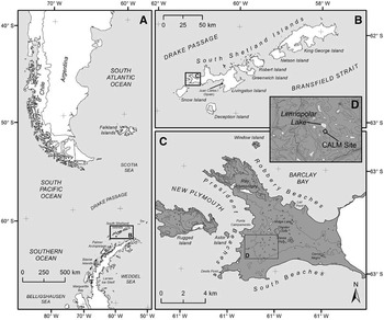
One of our contributions to these efforts, among others, was to establish a new CALM site in the Antarctic Peninsula region. Livingston Island was selected because it lies near the climatic boundary of permafrost (e.g. Bockheim Reference Bockheim2006, Vieira et al. Reference Vieira, Bockheim, Guglielmin, Balks, Abramov, Boelhouwers, Cannone, Ganzert, Gilichinsky, Gotyachkin, Lopez-Martinez, Meiklejohn, Raffi, Ramos, Schaefer, Serrano, Simas, Sletten and Wagner2010). Therefore, a CALM site in this area would help not only to increase limited presence of the CALM monitoring network in Antarctica, but also to obtain a complete record of the Active Layer Thickness (ALT) and ground temperature regime in the South Shetland Islands and in particular on Livingston and Deception islands. In this study, it was hypothesized that this CALM site would be one of the most sensitive permafrost sites to global warming. Permafrost has been monitored on the Hurd Peninsula on Livingston Island since 2000 and on Deception Island since 2006 (e.g. Ramos et al. 2008, Reference Ramos, Hasler, Vieira, Gruber and Hauck2009a, Reference Ramos, Vieira, Blanco, Gruber, Hauck, Hidalgo and Tomé2009b, Ramos & Vieira Reference Ramos and Vieira2009, Vieira et al. Reference Vieira, Bockheim, Guglielmin, Balks, Abramov, Boelhouwers, Cannone, Ganzert, Gilichinsky, Gotyachkin, Lopez-Martinez, Meiklejohn, Raffi, Ramos, Schaefer, Serrano, Simas, Sletten and Wagner2010). Under the aegis of the LIMNOPOLAR project (Toro et al. Reference Toro, Camacho, Rochera, Rico, Bañón, Fernández-Valiente, Marco, Justel, Vincent, Avendaño, Ariosa and Quesada2007), we installed a new CALM site near the shore of Limnopolar Lake (62°38′59.1″S, 61°06′16.9″W) on the Byers Peninsula (Fig. 1), Livingston Island (de Pablo et al. Reference de Pablo, Ramos, Vieira and Quesada2010, unpublished data). This peninsula lacks orographic barriers in the north, rendering it an excellent location for detecting regional climate changes (Turner et al. Reference Turner, Lachlan-Cope, Colwell, Marshall and Connolley2007, Reference Turner, Bindschadler, Convey, di Prisco, Fahrbach, Gutt, Hodgson, Mayewski and Summerhayes2009).
Location map of the Limnopolar Lake CALM site near the south-east shore of Limnopolar Lake (D) on Byers Peninsula (C), Livingston Island (B), Antarctica (A). Topographic contour lines on inset D every 20 m.

Since 2001, the LIMNOPOLAR project has focused on the study of Limnopolar Lake and its catchment area in order to reconstruct the Holocene palaeoclimate and to conduct interdisciplinary studies of modern processes. The location of the Limnopolar CALM site provides a better geological framework for surveying than most other locations in the Antarctic Peninsula region, which are commonly limited by: a) coarse sedimentary and/or rocky terrains, limiting measurements of ALT by mechanical probing, or b) anomalous geothermal locations, such as those on Deception Island, limiting their use for climate research.
Changes in ALT enable the detection of permafrost degradation as a reaction to climate change. However, in order to evaluate this, long-term data series are necessary. This paper reports the baseline obtained for the Limnopolar Lake CALM site, which will enable future changes on the Byers Peninsula, to be quantified. The 100 x 100 m CALM site was installed on sedimentary materials, at about 75 m a.s.l. (de Pablo et al. Reference de Pablo, Ramos, Vieira and Quesada2010), a similar altitude to the Crater Lake CALM site on nearby Deception Island (e.g. Ramos et al. Reference Ramos, Vieira, Blanco, Gruber, Hauck, Hidalgo and Tomé2008), allowing for reasonable comparison.
Active layer thickness and soil penetration resistance was measured once a year at the end of the thaw season, at all the nodes of the grid (spaced at 10 m). Concurrently, we monitored air, surface and ground temperatures continuously throughout the year in order to determine the thermal state and evolution of the active layer (de Pablo et al. Reference de Pablo, Ramos, Vieira and Quesada2010). Data collected at the Limnopolar CALM site have enabled us to characterize the state and evolution of the active layer on Byers Peninsula, and consequently to make inferences about permafrost conditions. Here we present our initial results, obtained during the first two years of monitoring this CALM site (February 2009–February 2011), and discuss their implications on active layer state and short-term evolution.
Study site
The Limnopolar Lake CALM site is located on Byers Peninsula (62°34′35″ S, 61°13′07″ W), a 60.6 km2 glacier-free area in the western part of Livingston Island, South Shetland Islands (Fig. 1), Antarctic Specially Protected Area (ASPA) No. 126 (ATCM 2003, Quesada et al. Reference Quesada, Camacho, Rochera and Velázquez2009). Byers Peninsula is the largest non-glaciated area in the South Shetland Islands, although snow covers it for 7–8 months a year. Data acquired by a meteorological station installed in the Limnopolar Lake basin measured typical meteorological variables (Bañon Reference Bañon2001, Toro et al. Reference Toro, Camacho, Rochera, Rico, Bañón, Fernández-Valiente, Marco, Justel, Vincent, Avendaño, Ariosa and Quesada2007, Bañon et al. 2013). Total annual precipitation is estimated to be about 800 mm, mean air temperature -2.8°C, with extremes of -27.4 and 9.3°C. Mean summer air temperature at 1.7 m is 1°C (Bañón et al. Reference Bañón, Justel, Velázquez and Quesada2013), with daily extremes of 9.3°C and -8.5°C, (Bañon Reference Bañon2001, Toro et al. Reference Toro, Camacho, Rochera, Rico, Bañón, Fernández-Valiente, Marco, Justel, Vincent, Avendaño, Ariosa and Quesada2007, Rochera et al. Reference Rochera, Justel, Fernández-Valiente, Bañón, Rico, Toro, Camacho and Quesada2010). Mean wind speed is about 25 km hr-1, although speeds as high as 139 km hr-1 have been reported (Toro et al. Reference Toro, Camacho, Rochera, Rico, Bañón, Fernández-Valiente, Marco, Justel, Vincent, Avendaño, Ariosa and Quesada2007). These conditions suggest that this region is on the climatic limit of permafrost.
Byers Peninsula is dominated by a smooth undulated plateau at about 105 m a.s.l. forming small drainage basins, most of them including lakes (as many as 60), small water bodies, seepages, and/or ponds (Fig. 1). The highest points are at Cerro Start (265 m) and Chester Cone (188 m). The geology is mainly Upper Jurassic–Lower Cretaceous volcanic, volcanoclastic and sedimentary materials (both detritical and carbonates), as well as different intrusive igneous bodies and Quaternary sediments (López-Martínez et al. Reference López-Martínez, Thomson and Thomson1996). Periglacial, glacial, fluvial, and weathering processes affected the bedrock after the deglaciation of the Peninsula over 5000 years ago (Björck et al. Reference Bjork, Hiort, Ingolfsson, Zale and Ising1996, Toro et al. Reference Toro, Granados, Pla, Giralt, Antoniades, Galán, Martínez-Cortizas, Lim and Appleby2013) and have generated a mantle of gravels, sands, and debris, locally forming stone circles, polygonal terrains, patterned ground, and other periglacial landforms (López-Martínez et al. Reference López-Martínez, Thomson and Thomson1996, Reference López-Martínez, Serrano, Schmid, Mink and Linés2012). These features reflect the important role of periglacial dynamics and many of them are indicators of permafrost (López-Martínez et al. Reference López-Martínez, Thomson and Thomson1996, Serrano et al. Reference Serrano, Martínez de Pisón and López-Martínez1996).
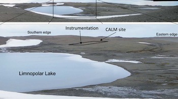
Limnopolar Lake is located at 70 m a.s.l. on the south-western part of the central plateau of Byers Peninsula. It is the main lake in a drainage basin of about 0.6 km2 that includes three smaller lakes (Rochera et al. Reference Rochera, Justel, Fernández-Valiente, Bañón, Rico, Toro, Camacho and Quesada2010). Limnopolar Lake is about 140 m in diameter and is located between small hills (Fig. 2). The northern and eastern edges of the lake (and of the Limnopolar basin) are marked by SE–NW and NE–SW trending hills, respectively, following regional morphological and tectonic lineaments (López-Martínez et al. Reference López-Martínez, Thomson and Thomson1996, Reference López-Martínez, Serrano, Schmid, Mink and Linés2012). Drainage of the lake occurs via a small stream along a deep and narrow gorge excavated between two smooth ridges at the north-east part of the lake and the basin. At the southern edge of the lake there is an alluvial plain formed by short and shallow braided channels (Fig. 2). Its surface is sandy-gravely and the water table is variable, being as shallow as 5 cm deep at the end of the thaw. The western edge of the lake is characterized by a plain of coarse sands to angular boulders, locally forming patterned ground (e.g. stone circles). No outcrops exist in the area except locally on the edge of the Limnopolar lake basin. The south-western edge of the lake is characterized by a hill with a regular east-facing slope (about 2 degrees), covered by unsorted materials (from rounded fine sands to coarse angular blocks) from shattered coarse sandstones, locally forming patterned ground. High water content and low penetration resistance soils and ponds are located in the area.
Panorama view, from the northern edge, of the Limnopolar Lake basin (top), where the Limnopolar Lake and the CALM site are visible (bottom).

Methods
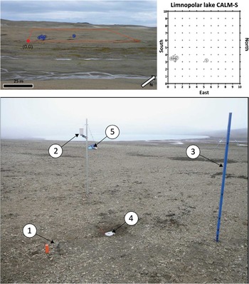
The Limnopolar Lake active layer monitoring site was installed in February 2009 (de Pablo et al. Reference de Pablo, Ramos, Vieira and Quesada2010) following the CALM protocol (Brown et al. Reference Brown, Nelson and Hinkel2000, Matsuoka & Humlum Reference Matsuoka and Humlum2003, Nelson et al. Reference Nelson, Shiklomanov, Hinkel and Christiansen2004, Nelson & Shiklomanov Reference Nelson and Shiklomanov2009), in order to monitor the evolution of ALT by mechanical probing at the end of the thaw season. The CALM site (Fig. 3) is a 100 x 100 m square grid with nodes spaced at 10 m intervals and marked in the field by orange-painted wooden stakes at the grid edges. The site extends from the highest to the lowest part of the flank of a small hill (Fig. 3) at the south-western shore of the lake. The slope inside the CALM site grid is generally < 3%, and the terrain shows differences in grain size, water table levels and geomorphological features between sites inside the grid.
Picture of the Limnopolar Lake CALM site (square), and CALM site diagram with location of the instruments (top): (1) borehole 1, (2) air temperature, (3) thermo-snow-meter, (4) surface temperature, and (5) borehole 2 (see Table I), and a nearest view of this instrumentation (bottom).

In order to complement ALT data (Fig. 4, Table I) and better understand climate forcing controls on the ground thermal regime, the CALM site includes air, ground surface and shallow borehole temperature data loggers, as well as snow thickness iButton sensor systems (de Pablo et al. Reference de Pablo, Ramos, Vieira and Quesada2010; Table II). These instruments were installed in February 2009, and the first data were recovered in February 2010, when the temperature sensors were replaced by others offering higher resolution (also iButtom type), and the measuring frequency was increased from four to three hours throughout the year (Table II).
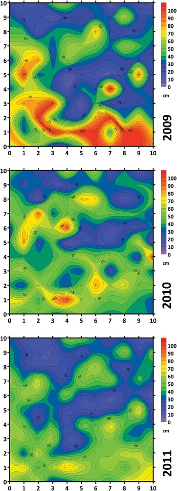
Active layer thickness (ALT) in the Limnopolar Lake CALM site measured in February 2009, 2010 and 2011 (Interpolation method: nearest neighbors).

Statistics of the Active Layer Thickness and soil penetration resistance measured (at 5 cm depth) at the end of thaw season in February 2009, 2010 and 2011. (n.d. no data)

Location and characteristics of the instruments installed in the Limnopolar Lake CALM site to monitor the active layer and its thermal evolution (numbers in first column correspond to sensors location in Fig. 3).

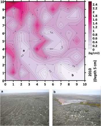
Site instrumentation consisted of two shallow boreholes equipped with temperature sensor-chains (the sensors were attached to a rope hanging inside a plastic tube 40 mm in diameter), one surface temperature sensor, a 1.6 m high mast equipped with temperature sensors to infer snow thickness (called a thermo-snow-meter) and one air temperature sensor (Fig. 3). Temperatures were measured every three hours with an accuracy of ± 0.5°C (iButton, 22L model, Maxim), except for the air temperatures, which were measured hourly with an accuracy of ± 0.2°C (TinyTag, Gemini, with external sensor). The instruments (Table I) were located inside the CALM grid (Fig. 3). In addition to these data, close to the end of the thaw period (depending on field logistics), and in parallel with ALT mechanical probing, soil penetration resistance was measured (Fig. 5, Table I) using a pocket soil penetrometer (ST207) and temperature was measured at 5 cm depth with a “K” thermocouple (Fluke) at each node of the grid (e.g. Nelson et al. Reference Nelson, Shiklomanov, Hinkel and Christiansen2004, Nelson & Shiklomanov Reference Nelson and Shiklomanov2009).
Map of the soil penetration resistance (SPR) (unconfined unconsolidated resistance) in the CALM site (top) measured in February 2010 by a pocket penetrometer ST207 (1 kg cm-2 = 1 N mm-2 = 0.10 MPa) (Interpolation method: nearest neighbours), and surface landforms observed on the areas with lower SPR values: a. patterned soils, and b. ponds.

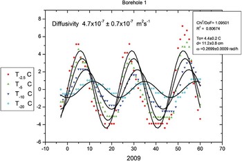
Ground thermal behaviour and thermal interactions between the weather, snow cover and ground properties were characterized. Temperature data from the thermo-snow-meter allowed us to infer snow thickness for the period February 2009–February 2011 (Fig. 6), using the procedure described in Danby & Hik (Reference Danby and Hik2007), based on an analysis of the daily temperature stability at each height, assuming that constant temperature is a consequence of snow cover. Moreover, freezing degree-days for near-surface ground (FDDs) and air (FDDa), and the n-factor (i.e. the ratio of the sum of degree days at the soil surface to that in the air) (e.g. Quinn et al. Reference Quinn, Assel, Boyce, Leshkevich, Snider and Weisnet1978, Assel Reference Assel1980, Klene et al. Reference Klene, Nelson, Shiklomanov and Hinkel2001) for the freezing periods of 2009 and 2010 were calculated (Fig. 7, Table III) to characterize the effects of ground insulation due to snow coverage. A thermal diagram of the ground at both boreholes and comparison with near-surface ground and air temperatures (Figs 6 & 8) provide complementary information to understand the thermal behaviour of the ground. In the Antarctic, this thermal behaviour mainly depends on the grain size and composition. In an initial approach, heat transport through the ground can be assumed to be conductive, especially if the ground is completely frozen and the ice blocks the pore space. Nevertheless, if the soil temperature is above the local water freezing point, other heat transport processes are possible and the conductive approach should be viewed with caution. All these effects can be taken into account by considering Apparent Thermal Diffusivity (ATD) (Hinkel et al. Reference Hinkel, Paetzol, Nelson and Bockheim2001) when assuming that the dominant means of heat transport is by conduction. ATD is the key which controls the heat exchange. Thermal diffusivity can experience considerable seasonal variations when thawing and freezing processes occur (Hinkel Reference Hinkel1997). When the temporal temperature series show a clear sinusoidal behaviour for a given frequency, it is possible to use the amplitude attenuation and the phase lag simultaneously for determining ATD and the characteristic periods by means of simultaneous fit process to different depths (Hinkel et al. Reference Hinkel, Outcalt and Nelson1990, Blanco et al. Reference Blanco, Hidalgo, Ramos and Vieira2010). We calculated the ATD for two different periods in the summers of 2009 and 2010 in order to analyse ground thermal behaviour, based on the temperature data obtained from borehole 1. This calculation uses the observed sinusoidal temperature signal as described in Blanco et al. (Reference Blanco, Hidalgo, Ramos and Vieira2010) and the fit procedure result is shown in Fig. 9.
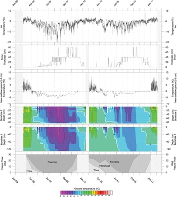
Data from 2009–11 period from the different instruments installed in the CALM site. From top to bottom: Air temperature, calculated snow thickness, surface temperature (5 cm depth), thermograms of borehole 2 and borehole 1, and number of monthly freeze-thaw days.

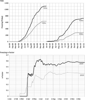
Freezing Degree-Days for air (FDDa) and near-surface ground (FDDs) evolution in 2009–11 period (top), and resulting freezing n-factor on a comparative plot (bottom).

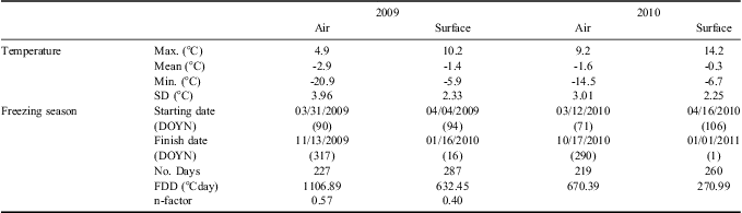
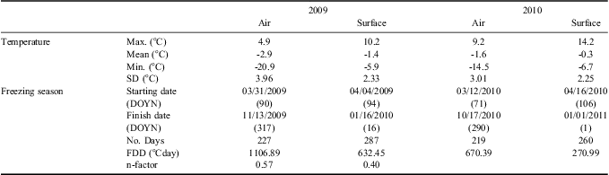
Statistics of the air and near-surface ground (5 cm depth) temperature data measured along 2009 and 2010. (DOYN: Day of the Year number)
Results
ALT at the Limnopolar Lake CALM site was measured in early February 2009, 2010 and 2011. Results are summarized in Table I, and Fig. 4 shows the ALT distribution on the CALM site grid. Mean average ALT at the CALM site was 47, 43, and 41 cm in 2009, 2010 and 2011, respectively, with maxima of 105, 99 and 85 cm, and minima of 8, 7, and 6 cm, respectively. The spatial distribution of ALT at the CALM site showed a similar pattern in 2009 and 2011, with the higher values in the eastern and south-eastern sectors, mainly corresponding to the lower altitude sector of the area, close to a stream bed. ALT in 2009 was generally thicker than in the subsequent years, but in 2011, although it was thinner, the thawed ground was more extensive. In 2010, ALT showed values intermediate between those of 2009 and 2011 and a more homogeneous spatial distribution.
In order to understand these results, in February 2010 we measured Soils Penetration Resistance (SPR) (Fig. 5). SPR measurements showed that its spatial distribution (Fig. 5) was similar to ALT distribution in 2009 and 2011 (Figs 4 & 5), indicating that the sites within the CALM grid which presented low SPR were, in general, the sites with a higher ALT. These sites were located in the eastern sector (where a pond is located) of the CALM grid, although a SW–NE corridor in the same area of the grid also showed higher ALT values in these years.
However, these data only provide information about the state of the ground (ALT and SPR) when it is measured, in late summer, but ground thermal evolution throughout the year is necessary to understand the dynamics of the active layer. Surface temperature was measured throughout the year by a sensor connected to a steel plate. However, since the surface temperature sensor failed in 2009, we have used data from the 5 cm deep sensor in the nearby borehole 1, in order to have comparable data for the whole period studied. These data show surface temperature throughout the thaw and freeze periods (Fig. 6), which enabled us to derive the number of days per month where the temperature remained above 0.5°C (thaw), below -0.5°C (freeze), and between 0.5°C and -0.5°C (interphase) (Fig. 6). An increase in thaw and interphase days was observed between 2009 and 2010 with small changes in the start and end dates of the freezing periods.
Snow thickness data from February 2009 to February 2011 shows (Fig. 6) similar winter cover, with snow reaching at least 40 cm thickness. The period with continuous snow cover started in mid May and lasted until early January. The period with over 40 cm of snow extended from early September to mid December in 2009, and from early August to mid November in 2010.
Mean air temperatures, measured above the snow layer (at 1.60 cm above the surface) were of -2.9°C and -1.6°C in 2009 and 2010, respectively (Table III). Air temperatures showed a mean value of -2.2°C for the whole period studied, but reached a maximum and a minimum of 14°C and -21°C, in early December 2010 and mid August 2009, respectively (Table III & Fig. 6). The air temperature range was smaller in 2010 than in 2009, with less extreme temperatures. Monthly patterns were similar for both years (Fig. 6). The air freezing period (when the daily mean air temperature remains below 0°C) started in April in 2009 and in mid March in 2010, and it finished in November of both years.
FDDs reached a maximum of 636°Cday in 2009, and 274°Cday in 2010, while FDDa reached 1106°Cday in 2009 and 725°Cday (Table III). In addition to higher FDD values in 2009 than in 2010, the increase in accumulated FDD throughout the year (Fig. 7) followed an approximately linear slope in 2009, but not in the autumn of 2010, which was more irregular. The calculated n-factor for freezing periods returned maximum values of 0.57 in 2009 and 0.40 in 2010 (Table III). Evolution of the freezing n-factor was different in 2009 and 2010, with a later and faster increase, and higher values in 2009 than in 2010. The increase in the n-factor stabilized about mid May and became continuous after early December.
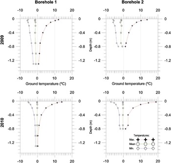
Temperature data at different depths in the two boreholes provided more in-depth knowledge about the thermal behaviour of the ground throughout the year. Thermal profiles showed similar behaviour at both boreholes, with less extreme temperatures (less warm and less cold) in 2009 than in 2010 (Fig. 8). Near surface ground temperatures showed strong fluctuations in 2009, but stabilized in 2010. Maximum, minimum and mean annual temperatures in borehole 1 in 2010 stabilized below 0.9–1 m. Ground temperature regimes were very different in each borehole (Fig. 8). In general, the ground remained frozen for longer periods at the different depths in 2009 than in 2010, with significant differences in the start and finish dates of the freezing period at different depths. It is interesting to highlight that the lower part of borehole 1 remained frozen in the middle of the summer in early February 2011, despite the warmer ground temperatures in winter in 2010.
Thermal profiles (temperature vs depth) of borehole 1 and borehole 2, in 2009 and 2010, showing maximum, mean and minimum temperatures.

Finally, the estimated ATD showed similar results for both periods, with values of 4.7 ± 0.7 x 10⁻⁷ m2 s-1 (Fig. 9) and 5.3 ± 1.8 x 10⁻⁷ m2 s-1, respectively. We should point out that the higher error value in 2010 was due to a lower time resolution (3 h) when compared to 2009 (1 h time resolution).
Sinusoidal fitting curves to temperature data from borehole 1 on a short period of three days in summer 2009, used to calculate Apparent Thermal Diffusivity (ATD) in Limnopolar Lake CALM site.

Discussion
The ALT measured in the period February 2009–February 2011 showed a decrease of 6 cm, from 47 cm in 2009 to 41 in 2011. This tendency was similar for the maxima and minima values measured, but higher for the maximum values (20 cm) than for the minimum ones (2 cm). The low ALT values in some places (minimum values) could have indicated certain artefacts, such as the measurement of rock depth rather than ice-cemented sediments of the permafrost. However, the measurement method included repeated measurements at each node to obtain the mean value, and we also repeated the measurements when we suspected the presence of rocks in the ground. Thus, changes in the measurements during the study period allowed us to discard the presence of rocks and thus discard the possibility of important errors in the measurement method.
The first two years of continuous monitoring of the active layer at the Limnopolar CALM site have provided information on interannual variability in active layer thickness, temperatures, soil resistance to penetration, snow thickness and air temperatures, FDD and the n-factor. Air temperature showed a similar pattern throughout the year in both 2009 and 2010, but with less extreme temperatures in 2010. The consequences of warmer air temperatures in this year included a lower number of freeze and thaw days (Table III, Fig. 5) and a warmer near-surface ground temperature. Air temperature evolution is also related to the evolution of snow cover, because stable snow cover starts when the air temperature remains below 0°C. Conversely, we observed that snow cover started to disappear when the temperature became less variable and approached near or above 0°C (Fig. 6). Moreover, when the snow melted there was a increase in near-surface and deeper ground temperatures (Fig. 6), firstly indicating the insulating effect of snow cover on the surface and ground temperatures during the winter, and secondly, the advection of warm water in the soil during the snow melting period. FDDa showed higher (absolute) values than FDDs, which could be evidence of insulation between the air and the ground, produced by the snow layer, in a similar manner to that observed in other cold and snowy regions (e.g. Karunaratne & Burn Reference Karunaratne and Burn2003).
The end of air freeze periods was associated with a reduction in snow thickness, and when the snow layer disappeared, there was a distinct increase in near-surface and deeper ground temperatures (Fig. 6). At this point, the ground surface temperature increased to nearly 0°C and remained constant for weeks, due to the warm, melting and isothermal snow pack. This process occurred in early December in 2009 and in late October in 2010, a difference related to the colder conditions in 2009 than in 2010.
The end of the thaw season on the air temperatures (when daily MAAT remained positive) also coincided with the end of the near-surface ground thaw season (Fig. 6), since there was no insulating snow layer. A clear example of this occurred in April 2009, when the air temperatures dropped below 0°C and the near surface ground immediately froze (Fig. 6).
Thermograms from borehole 1 and borehole 2 reflect the colder conditions in 2009, since the ground remained frozen and colder for longer in 2009 than in 2010 (Fig. 6). The freezing season started in early April in 2009 and finished in mid February 2010. However, although in 2010 the freezing season started in late April, it finished in early December 2010. The ground freezing season in 2009 lasted c. 10 months in 2009 and c. 8 months in 2010. These borehole temperatures showed three relevant behaviours: 1) in 2009, the ground was warmer between mid February to late May than in 2010, 2) there were differences in the start and finish of the thaw and freeze periods at different depths in each borehole, mainly in 2009, and 3) there were low and stable temperatures in borehole 2 at a depth of about 90 cm.The first observed behaviour may be related to the modifications in the terrain during drilling, as reported for other boreholes we drilled on Livingston and Deception islands (e.g. Ramos et al. Reference Ramos, Vieira, Blanco, Gruber, Hauck, Hidalgo and Tomé2008, 2009), as well as to small differences in local stratigraphy and material properties (mainly granulometry and porosity), since the boreholes were drilled at different locations inside the CALM site. The second behaviour could be related to stratigraphical differences (e.g. composition, granulometry, density, etc.) which could help the flow of sub-surface water during the thaw period, due to infiltration of snowmelt water. This is also consistent with the measured ALT and SPR spatial distributions described earlier in this paper, as well as other field observations such as the presence of a) low-scale geomorphological features (patterned ground), b) soft terrains, c) ponds, and d) shallow saturated horizons (Fig. 8). One possible explanation would be the existence of runoff at selected depths at the end of the thaw, which would coincide with our field observations regarding the location of the ground water saturation level (locally as shallow as 5 cm deep), and the gentle slope in the CALM-S site (about 2°). This effect, mainly visible in 2009, could also have been due to important modifications in the terrain caused by the drilling, or to differences in the water supply from snow melting or precipitation. However, to study the local hydrology is not the objective of the research presented here. For that reason, further detailed research should be done focused on describing the geological characteristics of the terrain and on determining the existence of this subsurface runoff. Finally, the third behaviour observed in the borehole thermograms could be the result of the stabilization of ground temperatures c. 2 years after the end of drilling. Temperature stabilization was visible in borehole 1, which was the deeper borehole. The depth at which the temperature remained constant was about 90 cm below the surface, which could be the depth of the active layer at this point, also indicated by the ALT maps (Fig. 4). We have not yet been able to confirm that this is the permafrost table since temperatures did not remain below 0°C for two consecutive years (Fig. 8), but a longer data series should make this determination possible.
In borehole 1, the depth of seasonal freeze-thaw was c. 90 cm and the thermal profile for borehole 2 suggests a similar value (Fig. 8). These values seems to indicate a greater depth than the mean thaw depth measured in early February for the entire CALM site (c. 45 cm) obtained by mechanical probing. However, the results are reasonable since thaw depth measured by mechanical probing in early February in the vicinity of each borehole was similar to the depth derived from thermal data for both years, February 2010 and February 2011 (Fig. 4). Thus, here we could conclude that the mechanical probing method provides accurate results, comparable to our thermal analysis of the active layer (Figs 6 & 8), as well as to the mean value of the ALT (about 30 cm) proposed for Byers Peninsula by Serrano et al. (Reference Serrano, Martínez de Pisón and López-Martínez1996). However, the spatial analysis of ALT and the ground temperature time-series showed that there was very variable thickness in both space and time of thaw penetration. Consequently, a detailed analysis of the terrain characteristics (granulometry, lithology, density, etc.) is required in order to understand the spatial distribution of ALT and the ground thermal behaviour.
The data obtained indicates that the differences observed in ALT for the period 2009–11 seem mainly to be due to interannual variability in air temperature (Fig. 4), which also seems to constrain the snow cover. In February 2009, the active layer was about 49 cm deep, although the eastern and southern sectors of the CALM site showed values that reached about 100 cm.We do not have air temperature data for the CALM site for the previous winter, but the meteorological data acquired at the Spanish Antarctic Station Juan Carlos I (on Hurd Peninsula, Livingston Island) indicated a warmer than average winter. The following year, when we measured the ALT in February 2010, the active layer had a mean thickness of 43 cm, but this greater thickness was only located in a few spots. This difference in the ALT distribution with respect to the previous year could be related to colder air temperatures in 2009, and to a longer period of snow cover. In fact, snow cover probably insulated the ground from the air in the spring-summer period (Fig. 6), a possibility which is supported by the analysis of the freezing n-factor.
Finally, in February 2011, we obtained a mean value of ALT of 41 cm with substantial variability within the CALM site grid. Maximum thickness spanned 90–100 cm, and was located mainly in the eastern and southern sectors (Fig. 4). This pattern was similar to the pattern observed in February 2010. This result is also supported by a reduced freezing season in 2010, with a shorter period of snow cover and lower values of freezing n-factor, indicating that the ground was less insulated and the period of interphase was longer (Fig. 6).
The spatial pattern of greater thaw depths in February 2009 and February 2011 was similar to the spatial pattern of SPR measured in February 2010. In general, the areas with lower SPR were the same ones where we measured higher ALT and where we also observed small-scale geomorphological features such as patterned ground and alignments of particles by size. Finally, the areas of low SPR were also those which presented soft terrain and shallow saturated horizons, although we will need to consider and test the role of ice segregation, cryoturbation, gelifluction and cryo-creeping.
The ATD values for the thaw periods (Fig. 9) were 4.7 ± 0.7 x 10⁻⁷ m2 s-1and 5.3 ± 1.8 x 10⁻⁷ m2 s-1, respectively, which are consistent with sedimentary materials and soils with significant water content (e.g. Campbell & Norman Reference Campbell and Norman2000), since the water thermal diffusivity is about 1.39 x 10⁻⁷ m2 s-1 and sand thermal diffusivity is about 11.5 x 10⁻⁷ m2 s-1. Therefore, the ATD of the ground in the borehole 1 was also consistent with the presence of liquid water in the ground, which could flow downslope due to the local gentle slope of the CALM site, and occasionally, also under a frozen level in the upper part of the soils, as could be inferred from thermograms. Groundwater flow over the permafrost has also been reported by Serrano et al. (Reference Serrano, Martínez de Pisón and López-Martínez1996), and our observations are consistent with this, and with its important effect on local hydrology in polar regions as indicated by Woo & Carey (Reference Woo and Carey1998).
This research on the evolution of the active layer at the Limnopolar CALM site over the period 2009–11 has revealed a clear interannual variability, with active layer thickness decreasing from 47 to 41 cm, with a concurrent increase in the mean average air temperatures from -2.9°C to -1.6°C. On the other hand, although a reduction in ALT in this period was observed, our data still do not confirm the presence of permafrost above 1.3 m below the surface. The upper limit of the permafrost was not detected during 2009–11 study period either by thermal analyses of temperature data acquired by sensors installed in the boreholes or by direct ALT mechanical probing. However, the thermal profiles (Fig. 7) could indicate the presence of permafrost between 1 and 1.3 m deep, but a deeper borehole would be necessary to solve these questions.
An understanding of the relationship between ALT and the weather and geological characteristics of the Limnopolar Lake CALM site constitutes an important tool for extrapolating to other sites on the Byers Peninsula. In our opinion, the change of the ALT could be important for Limnopolar Lake and other lakes on the Byers Peninsula. Permafrost and active layer melting could provide the water source for these lakes, together with snow and rain precipitations, and runoff. Understanding the role of each of these water sources would be difficult without also having an understanding of variability in the ALT at the Limnopolar Lake CALM site. Thus, with this study we have established the baseline for future comparative analyses and trend studies.
Conclusions
Two years of monitoring at the Limnopolar Lake CALM site on Byers Peninsula have provided data on the frost conditions and hydrological dynamics in a remote and poorly studied Maritime Antarctic site. Controls of weather, snow cover and soil properties on the thermal regime at the monitoring site have been identified, allowing for the following conclusions:
• The mean average thaw depth in February 2009–11 was about 44 cm in the study period, showing a degree of variability probably related to different annual weather conditions, based on ALT measurements made by mechanical probing.
• The active layer could reach thicknesses of up to 90–100 cm, based on analysis of ground temperature data, but we could not confirm that this was actually the depth of the permafrost upper limit.
• ALT was closely related to air temperatures throughout the year (colder during 2009), but was mostly controlled by snow cover, and the insulation that it provides between the air and the ground surface, as can be inferred from the calculated FDD and n-factor.
• The estimated ATD apparent thermal diffusivity suggests an influence of water content in the soils (sands).
Acknowledgements
This research was possible thanks to POL2006-006635, CTM2008-02042-E/ANT, CTM2009-10165, and REN2000-0435-ANT projects, supported by Science and Technology Ministry (Spain). The authors thank the Spanish Polar Committee, the Spanish Army and crew of the Las Palmas Oceanographic Research and Logistical Ship, and the Maritime Technology Unit (UTM, CSIC) for their help that made the fieldwork on Byers Peninsula possible. Special thanks to the mountain guides, for their assistance during the fieldworks. This paper was published with the financial support of the grant CTM2011-12973-E from Ministerio de Ciencia e Innovación (Spain)