1. Introduction

Sea-ice concentration in the Antarctic is subject to great variability, through both dynamic and thermodynamic forcing. Inlra-annual variability in the sea-ice concentration may be linked to the semi-annual oscillation of the Antarctic circumpolar trough, as the trough and sea-ice edge cross twice yearly, once in autumn as the sea ice advances, and again in spring as the ice retreats and the circumpolar trough advances north. During the spring retreat, the mean wind field over the ice will effectively change from a westerly to an easterly, and conversely, there will be a change from a dominant easterly to a westerly wind regime over the pack in autumn. This has implications for the sea ice, as with a westerly flow the Ekman drift will have a northerly component, causing divergence with in the pack. Likewise, an easterly wind will result in a southward, and hence convergent, sea-ice drift. in spring and summer the easterlies will aid in the rapid retreat of the sca-icc edge, and may cause greater congestion with in the pack itself. Likewise in autumn and winter, the westerlies will assist in the expansion of the sea-ice extent, and may also result in a more open pack that is susceptible to atmospheric and oceanic forcing.

Despite the possibility of such strong interactions, the relative time-scales of the sea ice, wind stress and temperature variability are unknown. One might expect that the sea-ice concentration would show an inertia to changes in the wind field because of its large mass and keel drag, and because the pack may move as one unit under spatially homogeneous conditions. Hence, in the longer time-scales, sea-ice concentration may display greater variability than the wind stress. As the concentration may also react slowly to changes in the surface air temperature, either because existing high concentrations prevent further freezing or because cold ocean temperatures moderate the melting due to a warm atmosphere, sea-ice concentration may also show more variability in longer time-scales than the surface air temperature. Hence, one might expect the variability of the sea-ice concentration to be biased towards longer time-scales than both the wind stress and the air temperature. Stich a bias is commonly known as a “red shift” in the frequency spectra.

The extern of any such red shift would not be expected to be similar over the entité sea-ice pack. Differing sea-ice (Ackley, 1991; Reference Gloersen, Campbell, Cavalicri, Comiso, Parkinson and ZwallyGloersen and others, 1992; Reference ParkinsonParkinson, 1994) and atmospheric (Reference Jones and SimmondsJones and Simmonds, 1993) conditions with latitude would suggest that the variability of the sea-ice concentration will differ with distance from the Antarctic continent.

2. Method

Daily winds and the temperature at 2 m above the surface were obtained on a 2.5° by 2.5° grid spacing from the European Centre for Medium-range Weather Forecasting (ECMWF) analyses for the years 1988-94. Wind slress was estimated by using an exchange coefficient of 10⁻³ in the bulk aerodynamic formula. Sea-ice concentration data from the U.S. Defense Meteorological Satellite Program's Special Sensor Microwavc/Imager for the same period were converted from 25 km resolution to the ECMWF grid. All data were then detrended by removing the first 14 waves of the annual cycle, effectively filtering out cycles with periods greater than 26 days. The residual was then separated into three “seasons”, each 122 days long. These cover the sea-ice growth phase from March to June (MAMJ), the months from July to October (JASO) and the decay stage from November to February (NDJF), and capture the sea-ice concentration maxima and minima belter than do the four standard climatological seasons. The temporal spectra of these seasonal data were determined, and the mean percentage of the variance explained (VE) by each wavenumber was calculated at every gridpoint for the 7 year period, 1988-94.

Fig. 1.

Bands used for the calculation of mean VE for the period July October. Lightest shade is the ice-edge band, darkest is the coastal band.

Spatial averages of the VE for the sea-ice concentration, wind stress and surface air temperature were made for each wavenumber over six latitudinal bands, the first at the ice edge (IE) and the second one gridpoint further south (IE2). The two central bands were constructed from, firstly, all those gridpoints at least two gridboxes south of the ice edge and two gridboxes from the coast (CP2), and secondly, a similar area which was three gridboxes from both coast and open water (CP3). The two coastal bands were constructed from the sea-ice gridpoints adjacent to the coast (CB), and those one gridbox further north (CB2). Figure 1 shows the latitudinal bands used for the JASO season. The NDJFand MAMJ bands (not shown) only have the central pack bands in the Ross and Wcddell Seas, as well as having some overlap in the ice-edge and coastal bands in the Amundsen, Bellingshausen and East Antarctic regions.

To calculate the statistical significance of sea-ice biases towards the longer time-scales compared to the spectra of stress and temperature, the difference of the VE in the 2-7 and 20-25 day periods in each year was calculated for each parameter, band and season. The hypothesis that this value for the sea-ice concentration would be less than that of the wind stress and surface air temperature (i.e. have a stronger red shift) was tested using the one-tailed t test.

3. Results

To test whether the sea-ice concentration displays a red shift from that of surface air temperature and wind stress, Figure 2 shows the JASO mean VE over the entire pack for frequency windows corresponding to periods of 2-7, 8-13, 14-19, 20-25 and > 25 days. (These correspond to wavenumbers 6 0-17, 16-9,8-7,6-5 and 4-1, respectively.) The spectrum of surface air temperature displays a red shift from that of the wind stress. The sea-ice concentration displays an even greater bias towards the longer time-scales when compared to the wind stress. For example, 17% of the temporal variability in the sea-ice concentration is explained by the window with periods of 20-25 days, whilst the temperature and wind stress have VEs of only 10% and 5%, respectively. By contrast, in the “synoptic” (2-7 d) window these values are 34%, 45% and 68%.

Fig. 2.

Mean VE (%) over the sea-ice zonefor July October wind stress (τ), temperature at 2 m (T02) and sea-ice concentration (Cone). Window 1= periods > 25 d,2 = 20-25 d, 3 = 14-19d,4 = 8-13d, 5 = 2-7d.

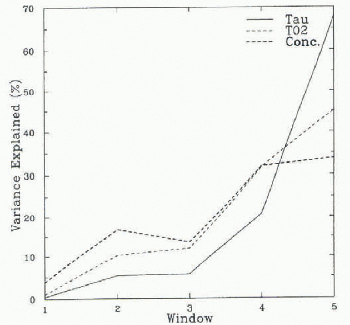
With such a clear indication of the red shift in the JASO mean case, we present the full frequency spectra for selected bands in each of the three seasons. A summary is presented in Table 1.

MAMJ

Mean VEs over the sea-ice bands IE and CB for MAMJ are shown in Figure 3. A weakened longwave bias of the sca-ice concentration compared to the near-surface temperature is apparent at the coastal gridpoint (fig. 3b). This may stem from several factors. As the ice edge and atmospheric convergence line (the centre line of the circumpolar trough) cross, the coastal bands are influenced by strengthening easterlies. These would reduce the divergence in the coastal bands (particularly the CB2 band, where the katabatic influence is weaker), whilst inducing much ridging and rafting. The exposed open water would then be susceptible to refreezing due to the lowering surface air temperature; this would not be instantaneous, however, as the competing strong easterlies and katabatics would force the frazil ice to the lee of any lead. Such competition on shorter time-scales would result in more synoptic variability, and thus smaller red shift.

Table 1.

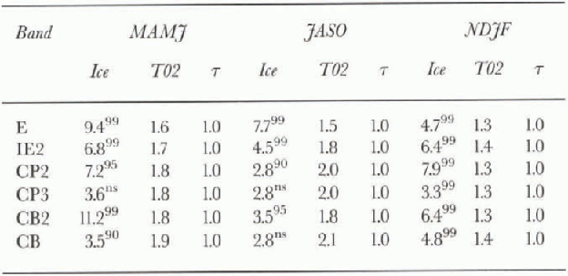
Red shift of the spectra in the latitudinal bands standardised by the wind stress

The large red shift in the outer pack reflects the change in the ice and atmospheric conditions as the atmospheric convergence line and the sea-ice edge cross, with near-surface temperatures often too close to freezing to cause any great concentration change, and the ice bands moving homogeneously.

JASO

Figure 4 shows a larger red shift occurring in the JASO outer pack than in the central and, to a lesser extent, coastal bands (not shown). This may be linked to the relative locations of the sea-ice edge and circumpolar trough, as during JASO the atmospheric convergence line is located to the south of the sea-ice edge, placing the outer pack in a general westerly, divergent, flow. The coastal regions would experience a mean easterly, thus inducing southward Ekman forcing upon the ice and working against the northerly forcing induced by new ice production. The central pack, however, may be under the influence of a more variable wind and temperature regime, inducing a broader spread in the VE spectrum. Under southerly winds, any open water created may be expected to rcfrcczc more rapidly as frazil ice is created (and pushed to the Ice of the lead) during the event, relaxing back into the lead as wind speeds reduce, whereas in the case of a northerly there may be less rapid ice production due to the warmer temperatures. Hence, the variability of the temperature forcing may be the key to the sea-ice concentration variance in the central pack, as suggested by the CP2 surface air-temperature and sea-ice concentration VE spectra (fig. 4b).

In the outer pack (fig. 4a), high sea-ice concentration VE is shown in the wavenumbers corresponding to periods of >20d. As for MAMJ, this may reflect the lack of formation of new ice due to “warm” air temperatures, and only slow melting due to the moderating effect of the cold ocean surface. It is also worth noting that similar long time-scales of variability are observed in the eddies associated with the Antarctic circumpolar current (Reference InoueInoue, 1985; Gillc and Kelly, 1996); however, it remains unclear if there is any link to the sea-ice concentration.

NDJF

Figure 5 shows the NDJF mean VE for each wave for the bands IE and CB2. The red shift is also strong in this season over the entire sea-ice pack, although it should be remembered that this is a time of relatively small sea-ice area, and hence bands may overlap. High VE values exist at the smaller wavenumbers for both bands, reflecting the gradual decline of the sea-ice concentration as warmer temperatures restrict refree/.ing of newly opened leads.

Fig. 3.

Average VE (%) for all wavenumbers for March-June wind stress (τ), temperature at 2 m (T02) and sea-ice concentration (Cone.) for (a) ice edge and (b) coastal band (gridpoint at the coast).

Fig. 4.

Average VE (%) for all wavenumbers for July-October wind stress (τ), temperature at 2 m ( T02) and sea-ice concentration (Cone.) for (a) ice edge and (b) central pack 2 (minimum two gridpoints from boundaries).

Fig. 5.

Average VE (%) for all wavenumbersfor November February wind stress (τ), temperature at 2 m ( T02) and sea-ice concentration (Conc.) for (a) ice edge and (b) coastal band 2 (second gridpoint from coast).

The total sea-ice-conccntration VE for wavenumbers greater than 30 (period ≤ 4d) is the highest for all seasons for both bands. Close to the ice edge, this may be due to the very open pack being highly susceptible to the cyclones that move over the ice edge as the circumpolar trough tracks southward. At the coast the divergent flow off the continent (often a result of combined geostrophic and katabatic processes; Reference Murphy and SimmondsMurphy and Simmonds, 1993) may well aid in the break-up and northward transport of newly formed coastal ice, resulting in large synoptic time-scale variability. When katabatics are not present, the prevailing easterlies, with the subsequent southward Ekman transport, may then force the ice coastward.

4. Concluding Remarks

For all seasons and latitude bands, a red shift occurs in the spectrum of the sea-ice concentration away from that of the wind stress and temperature at 2 m above the surface. The sea-ice concentration appears to be, in part, a low-pass filter of the high-latitude weather. For the wind stress, this may be a result of the large keel depth of the ice with respect to its sail height as well as the inertia of such large ice masses. It must also be noted that this study focuses on sea-ice concentration” which, conceivably, will not always change due to wind stress but may remain constant as the pack moves with a group velocity. The sea-ice concentration spectra also display a redder spectrum than does the surface air temperature. This may be due to the large energy loss required to cool the mixed layer to freezing point, the lack of open water in close pack to further freeze, or, for above-freezing temperatures, the moderating effect of the ice floating in the cold ocean water.

It is important to demonstrate that the response of the sea ice is found more markedly in the lower frequencies, and is above the noise level. To provide a summary of the “reddening”, Table 1 gives a measure of the red shift and its statistical significance for all seasons at all latitudinal bands. This has been constructed by considering the VE dillerence between the 2 7 and 20-25 day windows (WDIFF). These have been standardised by dividing the result into the WDIFF of the wind stress. Therefore, this value represents the strength of red shift for each parameter. Statistical significance is calculated on the difference between the WDIFF values for each of the three variables.

Results show that inJASO the outer bands of sea ice display greatest red shift away from the wind-stress and temperature spectra, with the central and coastal bands showing a smaller (and in some cases statistically insignificant) low-wavenumber bias, particularly from the temperature. Persistent very low temperatures during JASO cause new leads to refreeze quickly, resulting in a close relationship between the surface air-temperature and sea-ice concentration spectra. in NDJF, the latitudinal bands show strong and significant red shift in the central pack. This may be the result of the circumpolar trough moving to the north of the sea-ice edge, inducing persistent easterlies that force the sea ice southwards, causing congestion in the central Ross and Wcddell Sea packs. The bulk of the sea ice for this season, however, exists in the coastal and ice-edge bands, with the coastal bands having greatest (significant) red shift. It is worth noting that the sea-ice concentration also displays the highest VE, relative to the other seasons, in the shorter time-scales (<4d) for all bands. Finally, in MAMJ the peak red shift of the sea-ice concentration spectrum away from the temperature or wind stress occurs at the ice edge and at the coast, with both values statistically significant at 99%.

Our results aid not only in the general understanding of the Antarctic sea-ice pack, but also in quantifying aspects of the air-sea-icc interaction.