2.1 Phase field equation

In the phase field, a phase parameter $C$ is introduced such that $C=1$ and $C=0$ correspond to two distinctive phases, respectively. The evolution of the phase parameter $C$ traces out the deformation of the free surface. For the problem considered in this study, both diffusion and convection effects contribute to the development of phase field. The convective Cahn–Hilliard equation (Jacqmin Reference Jacqmin1999) is employed here to describe the evolution of the phase field,

(2.1) $$\begin{eqnarray}C_{t}+\boldsymbol{u}\boldsymbol{\cdot }\boldsymbol{{\rm\nabla}}C-M{\rm\nabla}^{2}{\it\phi}=0\quad \in {\it\Omega}\times T,\end{eqnarray}$$

where ${\it\Omega}$ is the geometric computational domain, with its boundary defined by $\partial {\it\Omega}$ , $T$ is the computing time duration, $\boldsymbol{u}$ represents the fluid velocity, $M$ is the phase field mobility and is taken as a constant in this study and ${\it\phi}$ is the chemical potential which is defined as ${\it\phi}={\it\delta}f/{\it\delta}C$ . The free energy density function, $f$ , which is a function of phase parameter $C$ , takes the following form,

(2.2) $$\begin{eqnarray}f(C)={\textstyle \frac{1}{2}}{\it\xi}{\it\gamma}{\it\alpha}|\boldsymbol{{\rm\nabla}}C|^{2}+{\it\xi}^{-1}{\it\gamma}{\it\alpha}\cdot {\textstyle \frac{1}{4}}C^{2}(1-C)^{2}\quad \in {\it\Omega}\times T,\end{eqnarray}$$

where ${\it\gamma}$ is the surface tension coefficient, ${\it\xi}$ is a measure of interface thickness and ${\it\alpha}=6\sqrt{2}$ is a constant.

Figure 1.

Schematic of the electrohydrodynamic RTI problem, the lower left corner is chosen as the original point of the coordinate. The electric field is in either horizontal or vertical direction.

2.2 Electric field equation

In dielectric materials, an external electric field polarizes the molecules, and the molecular dipoles so induced in return modifies the electric field. The resulting electric field is governed by the Gauss law $\boldsymbol{{\rm\nabla}}\boldsymbol{\cdot }({\it\varepsilon}_{r}(C)\boldsymbol{E})=q^{e}$ (Jackson Reference Jackson1999), where ${\it\varepsilon}_{r}(C)$ is the relative dielectric permittivity, $\boldsymbol{E}$ electric field intensity and $q^{e}$ free charge density. In this study, we focus on the fluids with small conductivity (e.g. benzene). For the case under consideration, the time scale of the flow $t_{c}=L_{c}/U_{c}$ ( $L_{c}$ being the length scale and $U_{c}$ the characteristic velocity) is much smaller than that of the charge relaxation $t_{{\it\sigma}}={\it\varepsilon}_{0}{\it\varepsilon}_{r}/{\it\sigma}(t_{c}\ll t_{{\it\sigma}}\text{ or }{\it\sigma}\ll {\it\varepsilon}_{0}{\it\varepsilon}_{r}U_{c}/L_{c})$ . As a result, the free charge may be neglected in the media ( $q^{e}=0$ ), and only polarized charges need to be counted for the electrical performance during the process.

Within the framework of electrohydrodynamics, the dynamic current is small, and hence the magnetic field is negligible. Also, the curl of the electric field is approximately zero ( $\boldsymbol{{\rm\nabla}}\times E=0$ ), which allows us to write $E=-\boldsymbol{{\rm\nabla}}V$ (where $V$ is the electric potential). Thus the governing equation of the electric field reduces to the Laplace equation (Tomar et al. Reference Tomar, Gerlach, Biswas, Alleborn, Sharma, Durst, Welch and Delgado2007; Hua, Lim & Wang Reference Hua, Lim and Wang2008; Lin, Skjetne & Carlson Reference Lin, Skjetne and Carlson2012),

(2.3) $$\begin{eqnarray}\boldsymbol{{\rm\nabla}}\boldsymbol{\cdot }({\it\varepsilon}_{r}(C)\boldsymbol{{\rm\nabla}}V)=0\quad \in {\it\Omega}\times T.\end{eqnarray}$$

The above equation governs both the bulk fluids and the diffuse interface. Indeed, one of the merits of phase field model is that, by introducing the phase parameter $C$ , the entire domain can be treated in a unified manner. This is in contrast with a sharp interface model where the two fluids must be treated separately, and a jump boundary condition is necessary at the fluid/fluid interface. Compared with the conventional Laplace equation $({\rm\nabla}^{2}V=0)$ , the permittivity ${\it\varepsilon}_{r}(C)$ in (2.3) is not a constant but a variable that depends on the phase parameter $C$ . Thus for a two-phase flow problem, such as the RTI, the permittivity ${\it\varepsilon}_{r}(C)$ varies spatially.

2.3 Flow field equation

The flow field is described by the governing equations of mass conservation and momentum balance equations. Both fluids are considered as incompressible, (Ding et al. Reference Ding, Spelt and Shu2007)

(2.4) $$\begin{eqnarray}\boldsymbol{{\rm\nabla}}\boldsymbol{\cdot }\boldsymbol{u}=0\quad \in {\it\Omega}\times T.\end{eqnarray}$$

The Navier–Stokes equations should be modified to allow for variable density and viscosity. For the present study, the external force includes the gravitational force, electrical force and surface tension force on the interface. Thus, the vector momentum balance equation takes the form of

(2.5) $$\begin{eqnarray}\displaystyle {\it\rho}(C)(\boldsymbol{u}_{t}+\boldsymbol{u}\boldsymbol{\cdot }\boldsymbol{{\rm\nabla}}\boldsymbol{u})=-\boldsymbol{{\rm\nabla}}p+\boldsymbol{{\rm\nabla}}\boldsymbol{\cdot }[{\it\mu}(C)(\boldsymbol{{\rm\nabla}}\boldsymbol{u}+\boldsymbol{{\rm\nabla}}\boldsymbol{u}^{\text{T}})]+{\it\rho}(C)\boldsymbol{g}+\boldsymbol{f}_{{\it\gamma}}+\boldsymbol{f}_{e}\quad \in {\it\Omega}\times T, & & \displaystyle \nonumber\\ \displaystyle & & \displaystyle\end{eqnarray}$$

where $\boldsymbol{f}_{e}$ denotes the electrical force (Tomar et al. Reference Tomar, Gerlach, Biswas, Alleborn, Sharma, Durst, Welch and Delgado2007; Hua et al. Reference Hua, Lim and Wang2008; Lin et al. Reference Lin, Skjetne and Carlson2012), $\boldsymbol{f}_{{\it\gamma}}$ accounts for the surface tension force, $\boldsymbol{g}$ is the gravity acceleration, ${\it\rho}(C)$ is the density of fluid, $p$ is the pressure and ${\it\mu}(C)$ is the viscosity. Note that (2.5) is valid for the entire computational domain, which is made possible by letting the physical properties be a function of the phase parameter $C$ . The surface tension force is expressed as

(2.6) $$\begin{eqnarray}\boldsymbol{f}_{{\it\gamma}}={\it\phi}\boldsymbol{{\rm\nabla}}C\end{eqnarray}$$

with ${\it\phi}$ being the chemical potential. The electrical force $\boldsymbol{f}_{e}$ can be calculated by taking the divergence of the Maxwell stress tensor (Saville Reference Saville1997):

(2.7) $$\begin{eqnarray}\displaystyle \boldsymbol{f}_{e} & \hspace{-2.0pt}=\hspace{-2.0pt} & \displaystyle \boldsymbol{{\rm\nabla}}\boldsymbol{\cdot }\left\{{\it\varepsilon}_{0}{\it\varepsilon}_{r}\boldsymbol{E}\boldsymbol{E}-\frac{1}{2}{\it\varepsilon}_{0}{\it\varepsilon}_{r}\left[1-\frac{{\it\rho}}{{\it\varepsilon}_{r}}\left(\frac{\partial {\it\varepsilon}_{r}}{\partial {\it\rho}}\right)_{T}\right]\boldsymbol{E}\boldsymbol{\cdot }\boldsymbol{E}{\bf\delta}\right\}\nonumber\\ \displaystyle & \hspace{-2.0pt}=\hspace{-2.0pt} & \displaystyle \boldsymbol{{\rm\nabla}}\boldsymbol{\cdot }\left[{\it\varepsilon}_{0}{\it\varepsilon}_{r}\boldsymbol{E}\boldsymbol{E}-\frac{1}{2}{\it\varepsilon}_{0}{\it\varepsilon}_{r}\boldsymbol{E}\boldsymbol{\cdot }\boldsymbol{E}{\bf\delta}\right]+{\it\varepsilon}_{0}\boldsymbol{{\rm\nabla}}\left(\frac{1}{2}\boldsymbol{E}\boldsymbol{\cdot }\boldsymbol{E}\frac{\partial {\it\varepsilon}_{r}}{\partial {\it\rho}}{\it\rho}\right),\end{eqnarray}$$

where $\boldsymbol{E}$ is the electric field intensity, and ${\bf\delta}$ the identity matrix. In the above equation, the first term on the right-hand side represents the electrical force due to the electrical charge, which sometimes is referred to as the Korteweg–Helmholtz force. The second one originates from the changes in material density, usually referred to as the electrostriction force density. This term is neglected in this paper as the fluid is incompressible.

2.4 Dimensionless parameters

In order to represent the density difference, the Atwood ratio $A=({\it\rho}_{2}-{\it\rho}_{1})/({\it\rho}_{2}+{\it\rho}_{1})$ is introduced, which is a key factor governing the RTI. The governing equations are normalized by the characteristic parameters: length $L_{c}$ , velocity $U_{c}=\sqrt{AgL_{c}}$ , and time $t_{c}=L_{c}/U_{c}=\sqrt{L_{c}/Ag}$ . Furthermore, the following dimensionless parameters are defined to simplify the analysis of the problem,

(2.8a−e ) $$\begin{eqnarray}Re=\frac{{\it\rho}_{m}\sqrt{L_{c}^{3}g}}{{\it\mu}_{m}},\quad We=\frac{{\it\gamma}}{{\it\rho}_{m}gL_{c}^{2}},\quad E_{b}=\frac{{\it\varepsilon}_{0}{\it\varepsilon}_{m}V_{0}^{2}}{{\it\rho}_{m}gL_{c}w^{2}},\quad Pe=\frac{{\it\xi}\sqrt{L_{c}^{3}g}}{M{\it\gamma}},\quad Cn=\frac{{\it\xi}}{L_{c}},\end{eqnarray}$$

where subscript $m$ ( $=\,1,2$ ) stands for the fluid with a greater value; for instance, ${\it\varepsilon}_{m}={\it\varepsilon}_{2}$ when ${\it\varepsilon}_{2}>{\it\varepsilon}_{1}$ . The Reynolds number (Re) describes the relative importance between the inertial (i.e. gravity) and the viscous force. Since gravity is a crucial force in the RTI, the significance of other forces is measured by dimensionless parameters in relation to gravity. The Weber number (We) reveals the relative magnitude of interface tension force and gravity force. The electrical Weber number $(E_{b})$ describes the ratio of the electrical over the gravity force. It is worth noting that for a vertical electric field $E_{b}={\it\varepsilon}_{0}{\it\varepsilon}_{m}V_{0}^{2}/({\it\rho}_{m}gL_{c}l^{2})$ . The viscosity and electrical permittivity ratios of the two fluids are represented by ${\it\lambda}_{{\it\mu}}={\it\mu}_{2}/{\it\mu}_{1}$ and ${\it\lambda}_{{\it\varepsilon}}={\it\varepsilon}_{2}/{\it\varepsilon}_{1}$ , respectively. For the phase field, two more parameters need to be defined: the Peclet number (Pe), which characterizes the ratio of the convective over diffusive mass transport and the Cahn number, Cn, which is defined as the ratio of the interface thickness over the characteristic length. For the problem in study, the two fluids are confined between two plates with a distance $l$ . This height $l$ is of importance and the characteristic length is chosen as $L_{c}=l/4$ , also we assume $w={\it\lambda}=l/4$ as the default value.

With the dimensionless parameters defined above, the governing equations can be normalized, namely,

(2.9a ) $$\begin{eqnarray}\displaystyle & \displaystyle C_{t}+\boldsymbol{u}\boldsymbol{\cdot }\boldsymbol{{\rm\nabla}}C-\frac{1}{Pe}{\rm\nabla}^{2}{\it\phi}=0, & \displaystyle\end{eqnarray}$$

(2.9b ) $$\begin{eqnarray}\displaystyle & \displaystyle \boldsymbol{{\rm\nabla}}\boldsymbol{\cdot }({\it\varepsilon}_{r}(C)\boldsymbol{{\rm\nabla}}V)=0, & \displaystyle\end{eqnarray}$$

(2.9c ) $$\begin{eqnarray}\displaystyle & \displaystyle \boldsymbol{{\rm\nabla}}\boldsymbol{\cdot }\boldsymbol{u}=0, & \displaystyle\end{eqnarray}$$

(2.9d ) $$\begin{eqnarray}\displaystyle A{\it\rho}(C)[\boldsymbol{u}_{t}+(\boldsymbol{u}\boldsymbol{\cdot }\boldsymbol{{\rm\nabla}})\boldsymbol{u}] & \hspace{-2.0pt}=\hspace{-2.0pt} & \displaystyle -\boldsymbol{{\rm\nabla}}p+\frac{\sqrt{A}}{Re}\boldsymbol{{\rm\nabla}}\boldsymbol{\cdot }[{\it\mu}(C)(\boldsymbol{{\rm\nabla}}\boldsymbol{u}+\boldsymbol{{\rm\nabla}}\boldsymbol{u}^{\text{T}})]+{\it\rho}(C)\boldsymbol{j}\nonumber\\ \displaystyle & \hspace{-2.0pt} & \displaystyle \hspace{-2.0pt}-\,\frac{1}{2}E_{b}{\it\beta}^{2}|\boldsymbol{{\rm\nabla}}V|^{2}\boldsymbol{{\rm\nabla}}{\it\varepsilon}_{r}(C)+We{\it\phi}\text{}\boldsymbol{{\rm\nabla}}C,\end{eqnarray}$$

where ${\it\phi}={\it\delta}f/{\it\delta}C$ and $f(C)=(1/2){\it\alpha}|\boldsymbol{{\rm\nabla}}C|^{2}Cn+(1/4Cn){\it\alpha}C^{2}(1-C)^{2}$ . Also, ${\it\beta}$ is a shape factor with ${\it\beta}=w/L_{c}$ for a horizontal electric field, and ${\it\beta}=l/L_{c}$ for a vertical electric field. The dimensionless density, viscosity and relative permittivity are further given by

(2.10a ) $$\begin{eqnarray}\displaystyle {\it\rho}(C) & \hspace{-2.0pt}=\hspace{-2.0pt} & \displaystyle (2AC+1-A)/(1+A),\end{eqnarray}$$

(2.10b ) $$\begin{eqnarray}\displaystyle {\it\mu}(C) & \hspace{-2.0pt}=\hspace{-2.0pt} & \displaystyle C+(1-C)/{\it\lambda}_{{\it\mu}},\end{eqnarray}$$

(2.10c ) $$\begin{eqnarray}\displaystyle {\it\varepsilon}_{r}(C) & \hspace{-2.0pt}=\hspace{-2.0pt} & \displaystyle C+(1-C)/{\it\lambda}_{{\it\varepsilon}}.\end{eqnarray}$$

2.5 Boundary and initial conditions

For the fluid flow field, no-slip conditions are imposed at the top and bottom walls, $\boldsymbol{u}=0$ and the Neumann conditions are applied at side boundaries, $\partial \boldsymbol{u}/\partial n=0$ . For the electric field imposed in the vertical direction, Dirichlet boundary conditions are applied on a pair of electrodes, $V=1$ at $y=l/L_{c}$ , and $V=0$ at $y=0$ , and Neumann conditions for the side boundaries, $\partial V/\partial n=0$ at $x=0$ and $x=1$ . For the horizontal electric field, the boundary conditions are different: $V=1$ at $x=0$ , $V=0$ at $x=1$ , and $\partial V/\partial n=0$ at $y=l/L_{c}$ and $y=0$ . For pressure, its normal derivatives are all set to zero, $\partial p/\partial n=0$ . The Neumann boundary conditions are imposed at all boundaries for phase field and chemical potential, $\partial C/\partial n=0$ , and $\partial {\it\phi}/\partial n=0$ ; this guarantees the conservation of total mass. Initially, the flow field is set zero everywhere, which means the system starts to evolve from quiescence. The initial interface is assumed to take a shape of a cosine wave, below which the phase parameter is set as $C=0$ and above which $C=1$ .

2.6 Numerical methodology

All the equations are discretized by the finite difference method and solved numerically for each time step. The detailed computational methodology is described elsewhere (Yang et al. Reference Yang, Li, Shao and Ding2014) and thus only an outline is given here. A collocated grid is used and the temporal terms in the above equations are discretized explicitly. Calculations start with the solution of the phase field $C$ . Then, the density, viscosity and dielectric constant are updated using (2.9). In the present model, all the parameters (the density ${\it\rho}(C)$ , viscosity ${\it\mu}(C)$ and permittivity ${\it\varepsilon}_{r}(C)$ ) are treated as linear functions of the phase parameter $C$ across the interface. The specific form of the function is insignificant for the problem under consideration since the interface is rather thin compared with the whole computational domain. The first-order derivative terms employ an upwinding scheme to increase the numerical stability. The Laplace equation for the electric field is discretized using a central difference scheme and solved by the method of successive over-relaxation (SOR).

A projection method (Yang et al. Reference Yang, Li, Shao and Ding2014) is employed to solve the Navier–Stokes equation together with the mass conservation equation and with the force terms obtained from the electric field. For a large density ratio, spurious currents may occur at the interface, which may cause numerical instability. Numerical experience suggests that the harmonic interpolation, $1/{\it\rho}_{i+1/2}=(1/{\it\rho}_{i}+1/{\it\rho}_{i+1})/2$ , is useful in preventing this numerical instability (Yang, Li & Ding Reference Yang, Li and Ding2013) and it is thus used in the present study. Having obtained the fluid flow field, the phase field is then solved again for the next time step. This procedure repeats itself until the preset time duration is reached. The time steps and grid sizes are so chosen to ensure the accurate and stable numerical solutions.

3.1 Model validation

Unless otherwise indicated, all the results in the following will be presented in dimensionless units introduced in the previous section. To validate our model, the classical RTI without electric field was simulated, and then compared against the available numerical results. The same parameters are chosen as given by Ding et al. (Reference Ding, Spelt and Shu2007). Specifically, the Atwood ratio $A=0.50$ , $Re=3000$ , the height $l=4w$ , surface tension is not considered and the fluids are assumed to be incompressible. In the present case of zero surface tension, the Cahn–Hilliard equation simply amounts to the interface tracking only. The initial interface being located in a rectangular domain $[0,1]\times [0,4]$ at $y(x)=2+0.1\cos (2{\rm\pi}x)$ , which represents a planar interface superimposed by a perturbation of wavenumber $k=1$ with an amplitude $0.1w$ . The top of the rising fluid and the bottom of the falling fluid are monitored, with the results presented in figure 2. As can be seen, the computed results from the present model agree well with those of Ding et al.

Figure 2.

Time evolution of the positions of rising and falling tips, along with the results given by Ding et al. Both time and position are dimensionless.

After validating the numerical model for the conventional RTI without an electric field, the next step is to verify its correctness with the presence of an electric field. To do so, the results from numerical simulations are compared against those by linear stability analysis for the growth rate of RTI in a horizontal electric field (see appendix A for detailed linear stability analysis). Substituting the parameters into (A 14), the results by linear stability analysis are obtained and shown in figure 3, where the numerical results from the present model are also given. For this case, the gravity is ignored, which is equivalent to removing the term ${\it\rho}(C)\boldsymbol{j}$ from (2.9d ). One detail needs to be clarified about the neglecting of gravity in this particular case. To maintain the same definition of the dimensionless parameters involving gravity (such as the Reynolds number), $g$ is kept as a constant and assigned a value of $g=9.8$ . The interface is assumed to be $f(x,t)=\text{e}^{st}A_{0}\cos (kx)$ , and the real part of $s$ represents the growth rate of the perturbation. As shown in figure 3, $s$ is negative, indicating that the instability is suppressed by the horizontal electric field. It is noted that the numerical data in figure 3 was obtained via the best fit of function $f(x,t)$ . As it can be seen, the numerical results compare well with those of the linear analysis, validating the correctness of numerical phase field model. It is worth pointing out that in order to compare with linear stability analysis, the initial amplitude of perturbation $A_{0}$ is set sufficiently small for it to fall into the linear region (i.e. $A_{0}\ll {\it\lambda}$ , ${\it\lambda}=2{\rm\pi}/k$ ). More comparisons between the numerical and linear results are presented in the subsequent sections.

Figure 3.

Comparison of the growth rates of interface perturbation predicted by linear stability analysis and by the present numerical model for horizontal electric fields imposed. Gravity and surface tension are ignored, and other parameters are listed in table 1. The growth rate is normalized by $t_{c}^{-1}=\sqrt{Ag/L_{c}}$ .

For convenience, a set of default parameters are defined and listed in table 1. These values of parameters were used in the results to follow unless otherwise indicated. In the present study, the Peclet number (Pe) is taken as a function of surface tension $Pe=2.5/{\it\gamma}$ . If the surface tension is zero, the Peclet number would lose its meaning and phase field simply tracks the interface evolution caused by convection.

Table 1.

Parameters used in calculations.

3.2 Stability analysis

3.2.1 Electrohydrodynamic RTI in a horizontal electric field

The effect of a horizontal electric field on the RTI is assessed in this section. It is known that a tangential electric field stabilizes the interface between two dielectric materials (Melcher & Schwarz Jr Reference Melcher and Schwarz1968). For the specific case of the RTI, according to the linear stability analysis, the horizontal electric field would suppress the perturbation on the interface (Barannyk et al. Reference Barannyk, Papageorgiou and Petropoulos2012). In the following, the numerical model described and validated above is employed to conduct the fully nonlinear analysis.

In the phase field model, the interface is represented by the contour of phase parameter $C=0.5$ . The initial perturbation is set as $y(x)=2+0.0025\cos (2{\rm\pi}x)$ . As the interface deformation evolves, the positions of ‘rising tip’ (i.e. bubble) and ‘falling tip’ (i.e. spike) are monitored. For the convenience of subsequent discussion, a parameter ${\rm\Delta}h$ is defined to quantitatively characterize the instability. This important quantity stands for the structure height, which is the difference between the positions, viz.

(3.1) $$\begin{eqnarray}{\rm\Delta}h=y_{r}-y_{f},\end{eqnarray}$$

where $y_{r}$ and $y_{f}$ measure the vertical positions of the rising and falling tips, respectively. A small ${\rm\Delta}h$ means the interface deformation is small, while a large value indicates a serve deformation.

The configuration being studied is shown in figure 1 with the electric field applied in the horizontal direction. For this case, both gravity and surface tension are considered. Computed results are plotted in figure 4(a), which shows the time change of structure height with different electric fields whose strength is characterized by the electrical Weber number $E_{b}$ . Clearly, the instability is driven by a competing mechanism between the gravity and the horizontal electric field, with the former destabilizing the interface and the latter (electric field) stabilizing it. For the field-free case ( $E_{b}=0$ ), the gravity effect dominates and the structure height grows continuously and the instability is aggravated. A weak electric field slows down the instability but does not suppress it, which is evident with the cases of $E_{b}=0.25$ . However, a strong electric field (i.e. a large $E_{b}$ ) overwhelms the destabilizing effect of gravity and completely suppresses the interface perturbation. For the cases considered, with a field strength of $E_{b}=0.4$ , the perturbation is suppressed by the horizontal electric field. Moreover, an oscillation occurs during the suppression process, which is also reported in a previous study (Cimpeanu et al. Reference Cimpeanu, Papageorgiou and Petropoulos2014). For an even stronger electric strength ( $E_{b}=0.8$ and 4.0), the perturbation decays faster and the period of oscillation becomes shorter. For a comparison, the linear analysis results (see appendix A) are also shown in figure 4; clearly, the numerical results are consistent with the linear analysis. From the computed data, one may readily construct a stability diagram demarking the stable and unstable regions, the boundary of which is defined by the critical voltage. According to the present calculations, the critical value of $E_{b}$ is 0.32. This is in consistency with the critical value of $E_{b}=0.3$ predicted by linear stability analysis (see appendix A for details).

Figure 4.

(a) Time evolution of structure height as affected by horizontal electric fields $(E_{b})$ . The electrical permittivity ratio of the two fluids is ${\it\varepsilon}_{2}/{\it\varepsilon}_{1}=3:1$ . Other parameters are the same as in table 1. Solid lines represent numerical results and discrete dots indicate linear analysis. (b) The electrical force distribution along the fluid–fluid interface. The scale bar measures the magnitude of the electrical force.

To provide a better physical insight into the suppression effect of a horizontal electric field, the distribution of the electrical force (which in this case is referred as the Korteweg–Helmholtz force) along the interface is plotted in figure 4(b). It is noted that the plotted electrical force is normalized by ${\it\varepsilon}_{0}|{\it\varepsilon}_{2}-{\it\varepsilon}_{1}|V_{0}^{2}/(2w^{2})$ , which is the force on a flat interface. In phase field representation, the fluid–fluid interface is characterized by a diffusive interface layer, whose thickness is defined by $0.01\leqslant C\leqslant 0.99$ ( $C$ is the phase parameter). This is in contrast with a sharp interface model across which flux experiences a jump. The electrical force given in figure 4(b) is calculated by integrating the force density across the thickness of the diffusive interface layer, whose shape is given by $y(x)=2+0.0025w\cos (2{\rm\pi}x)$ at the onset of the instability. Although the force distribution evolves with time, a snap shot at an instant provides useful information on how it affects the interface development. As it is seen in figure 4(b), the force is normal to the interface and points downwards. It is strong at the rising tips on the two sides of the domain, pushing the interface downwards. At the falling tip, on the other hand, the electric force is weak. Also, the fluids are incompressible and need to satisfy the constraint of mass conservation. As a result, the interface is pushed upwards. This is the mechanism by which a horizontal electric field suppresses the RTI.

The Korteweg–Helmholtz force is known being normal to the interface and pointing from the fluid with larger permittivity to the smaller one, thus the force depends on the relative values of the electrical permittivities of the two fluids. In the previous section, ${\it\varepsilon}_{2}>{\it\varepsilon}_{1}$ was discussed. The case of ${\it\varepsilon}_{2}/{\it\varepsilon}_{1}=1:3$ is considered here. Figure 5(a) shows the evolution of structure height with different electrical Weber numbers. The results are similar to the case of ${\it\varepsilon}_{2}/{\it\varepsilon}_{1}=3:1$ ; namely, a weak horizontal electric field slows down the instability and a field strong enough can completely suppress it. The electrical force along the interface is displayed in figure 5(b). In contrast to figure 4(b), the force in this case points upward, being the largest at the falling tip and gradually decreasing from the falling to the raising tip along the interface. Under the action of this electrical force (figure 5 b), the falling tip is pushed upward and the rising tip is squeezed downward due to the conversation of mass, thereby resulting in a suppression effect on the instability.

Figure 5.

(a) Evolution of structure height under the influence of horizontal electric fields $(E_{b})$ . The electrical permittivity ratio is ${\it\varepsilon}_{2}/{\it\varepsilon}_{1}=1:3$ . Other parameters are the same as in table 1. Solid curves – numerical results and discrete dots – linear analysis. (b) The distribution of the electrical force along the interface. The scale bar denotes the magnitude of the electrical force.

For both ${\it\varepsilon}_{2}/{\it\varepsilon}_{1}>1$ and ${\it\varepsilon}_{2}/{\it\varepsilon}_{1}<1$ , a horizontal electric field produces a suppression effect on the RTI. The suppression effect is also predicted by a linear stability analysis (see appendix A for details), where the effect of the electric field in the dispersion equation appears as ${\it\varepsilon}_{0}({\it\varepsilon}_{2}-{\it\varepsilon}_{1})^{2}E_{0}^{2}/({\it\varepsilon}_{2}+{\it\varepsilon}_{1})$ (see (A 14)). This term remains the same for both ${\it\varepsilon}_{2}>{\it\varepsilon}_{1}$ and ${\it\varepsilon}_{2}<{\it\varepsilon}_{1}$ , but it produces an opposite effect to gravity. The reason of comparing the two cases ( ${\it\varepsilon}_{2}/{\it\varepsilon}_{1}=3:1$ and $1:3$ ) is to indicate that the stability characteristic resembles each other for the two cases but the detailed action of the electric forces on the interface is different. Also, the interfacial morphology differs for the two cases, which may not be explained by linear analysis, as it will be discussed in § 3.3.

3.2.2 Electrohydrodynamic RTI in a vertical electric field

The electric field in different orientations has different effects on the interface instability. It is known that the electric field perpendicular to the interface would aggravate the instability (Taylor & Mcewan Reference Taylor and Mcewan1965). Recently this phenomenon is exploited to manufacture the micro/nano structure on thin polymer films (Wu & Russel Reference Wu and Russel2009). In this section, the effect of a vertical electric field on the RTI is discussed. Consistent with the previous section, the structure height is monitored during numerical simulation in order to quantify the instability. The case of ${\it\varepsilon}_{2}/{\it\varepsilon}_{1}=3:1$ is studied first, and the results are plotted in figure 6. Both numerical and linear analytical results are depicted in figure 6. As expected, they agree with each other when the structure height is small; and deviate from each other for a large structure height as the nonlinear effect comes into play. Clearly, both numerical and linear analytical results indicate that the vertical electric fields tend to enhance the RTI. The structure height accelerates higher in time with a vertical electric field, and the interface becomes more and more unstable with an increase in the electric field strength. The stability analysis in a vertical electric field can also be performed by a linear theory (see appendix B for details), which yields the same conclusion. In an attempt to uncover the mechanism for this effect, the electrical force distribution along the interface is depicted in figure 6(b). The force acts downward with a maximum at the falling tip and gradually reduces in magnitude along the interface to a minimum at the rising tip. For the vertical electric field, the electrical forces are normalized by ${\it\varepsilon}_{0}|{\it\varepsilon}_{2}-{\it\varepsilon}_{1}|V_{0}^{2}/(2l^{2})$ . Following the same line of argument as discussed in the above, the force distribution in figure 6(b) accelerates the downward motion of the interface at the falling tip and the upward motion at the rising tip due also to the conservation of mass, thereby enhancing the RTI.

Figure 6.

(a) Evolution of structure height under the action of vertical electric fields $(E_{b})$ . The electrical permittivity ratio is ${\it\varepsilon}_{2}/{\it\varepsilon}_{1}=3:1$ . Other parameters are the same as in table 1. Solid lines represent numerical results and discrete dots indicate linear analysis. (b) The electrical force distribution along the interface. The scale bar indicates the magnitude of the electrical force.

The case of ${\it\varepsilon}_{2}/{\it\varepsilon}_{1}=1:3$ is shown in figure 7(a), where similar results are obtained, that is, the RTI is enhanced and becomes stronger with a larger electrical Weber number. Electrical force along the interface at the initial occasion is plotted in figure 7(b). The orientation and the distribution of the electrical force along the interface both are almost opposite to those in the case of ${\it\varepsilon}_{2}/{\it\varepsilon}_{1}=3:1$ . The force points upwards with the largest value at the rising tip and the smallest one at that falling part, which, in combination with the requirement for mass conservation, results in an aggravation of the RTI.

Figure 7.

(a) Evolution of structure height under the action of vertical electric fields $(E_{b})$ . The electrical permittivity ratio is ${\it\varepsilon}_{2}/{\it\varepsilon}_{1}=1:3$ . Other parameters are the same as in table 1. Solid curves – numerical results and discrete dots – linear analysis. (b) The electrical force distribution along the interface. The scale bar denotes the magnitude of the electrical force.

3.3 Interfacial morphology of electrohydrodynamic RTI

The RTI usually evolves in the following pattern: one part of fluids falls downward (sometimes referred as ‘spike’) while the other rises up (i.e. ‘bubble’), with sometimes roll-ups appearing at the tip due to nonlinear interaction (Sharp Reference Sharp1984). In § 3.2, the stability of interface under the action of electric fields was discussed. The instability was quantified by the structure height difference between the rising and the falling tips. One key issue is the interfacial morphology of the RTI, which is the subject of this section. The interface exhibits various morphology patterns even with the same structure height. It is reasonable to conjecture that the electric field orientation and strength may play important roles in determining the evolution of the interfacial morphology. Here attention is focused on two aspects of the interfacial morphology, with one concerning the width of the ‘spike’ and/or the ‘bubble’, and the other the appearance of the roll-ups at the tip. As in the above, the influence of the horizontal and vertical electric field on the interfacial morphology will be discussed in separate sections below.

3.3.1 Interfacial morphology under the action of horizontal electric field

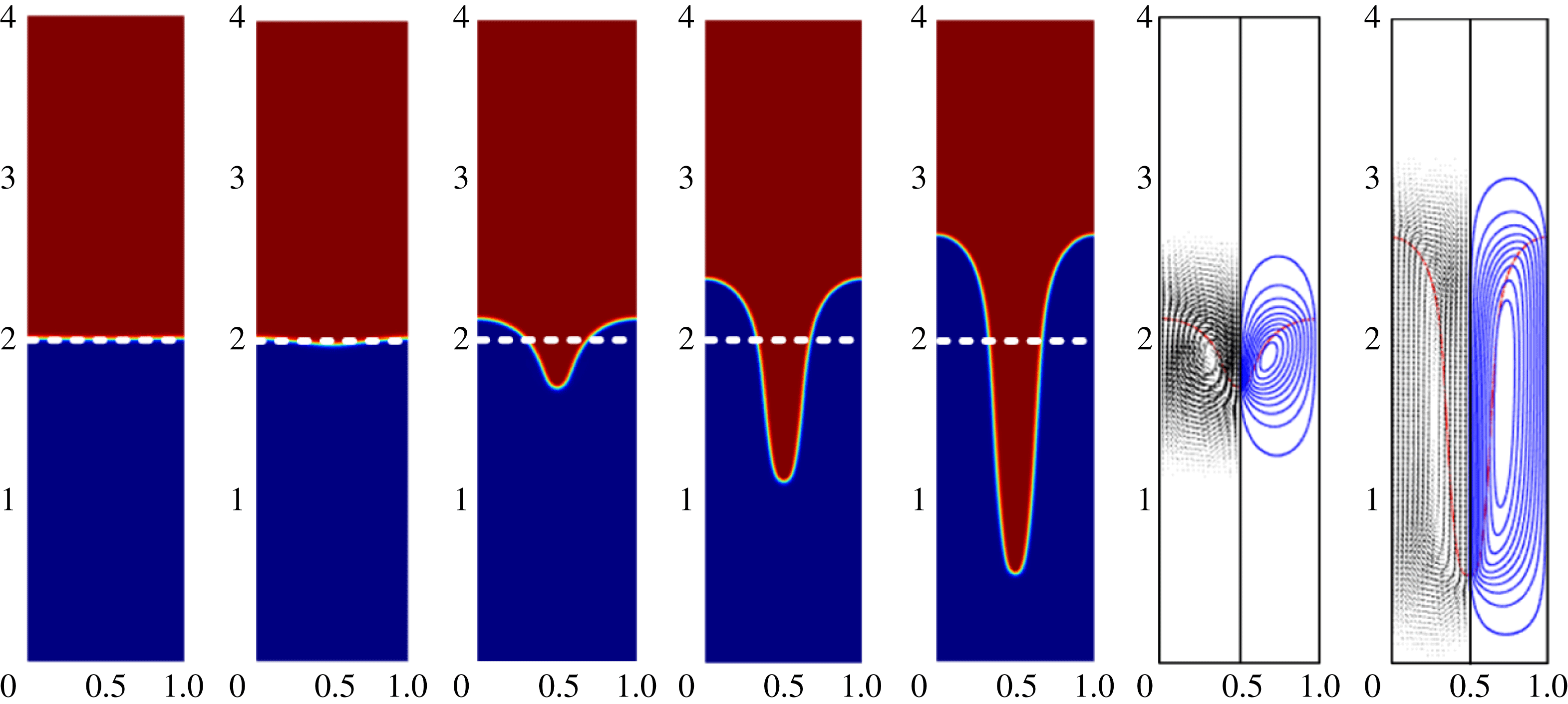
Some representative results of the interfacial morphology and flow field in the presence of horizontal electric fields are shown in figure 8. Specifically, figure 8(a) shows the evolution of the interfacial morphology and flow fields for $E_{b}=0.1$ , which is a relative small value. Initially, the flow is characterized by a relatively simple pattern, with the heavy fluid falling down at the centre and the light fluid rising up at the two sides. As time progresses, the tail forms around the ‘spike’ and the vertex starts to emerge. The interface evolves into an even more complex pattern as time continues. With an increase in field strength, as shown in figure 8(b) for the case of $E_{b}=0.2$ , the ‘spike’ is shorter and thinner compared with figure 8(a). The suppressing effect of a horizontal electric field on the RTI illustrated here can be explained by the same mechanism as discussed above. With a stronger field, the instability is weakened by the electrical force along the interface, and only a small part wedges into the light fluid to form a shorter and thinner ‘spike’. Comparison of figure 8(a) and (b) shows that the similar flow field is obtained except that the falling part is smaller with a stronger electric field. An even stronger electric field ( $E_{b}=1.0$ ) can completely suppress the instability, which is shown in figure 8(c). For this case, the interface undergoes an oscillation with a rather small amplitude and eventually becomes essentially flat.

Figure 8.

The RTI under the action of different horizontal electric fields: (a) $E_{b}=0.1$ , (b) $E_{b}=0.2$ and (c) $E_{b}=1.0$ . Other parameters are the same as in table 1. The dimensionless time for the panels, from left to right, are $t^{\ast }=0$ , 2.0, 3.0, 4.0 and 5.0. The dashed line represents the equilibrium interface. The vector flow field and streamline contours are plotted at right for $t^{\ast }=3.0$ and $t^{\ast }=5.0$ .

Appearance of fluid roll-ups is a common phenomenon associated with the RTI. The essential feature of the roll-up phenomenon is preserved for a weak electric field. This is clearly shown in figure 8(a) where two counter-rotating vortices are formed along the sides of the falling fluid stream. Similar results in the absence of electric fields were observed by other researchers (Tryggvason Reference Tryggvason1988; He et al. Reference He, Chen and Zhang1999; Guermond & Quartapelle Reference Guermond and Quartapelle2000; Ding et al. Reference Ding, Spelt and Shu2007). It is generally accepted that the roll-ups and vortices are caused by the secondary instability occurring at the interface between two fluids in motion (Daly Reference Daly1967). The secondary instability appearing along the side of the ‘spike’ causes the interface to ‘mushroom’, which increases the effect of traction on the ‘spike’ and as a result vortex forms (Sharp Reference Sharp1984). For inviscid fluids, this secondary instability is often referred as the Kelvin–Helmholtz instability (KHI). For two viscous fluids with different viscosities, the Yih instability dominates the secondary instability (Yih Reference Yih1967; Boomkamp & Miesen Reference Boomkamp and Miesen1996). This study considers another explanation for the roll-ups. According to the Bjerknes theorem (Thorpe, Volkert & Ziemianski Reference Thorpe, Volkert and Ziemianski2003), one source of the vorticity comes from the baroclinity, which is proportional to the cross-product of the density gradient and the pressure gradient, $\boldsymbol{{\rm\nabla}}p\times \boldsymbol{{\rm\nabla}}{\it\rho}$ . In an RTI system, the gravity is the driving force in absence of electric field. The pressure tends to distribute vertically and its gradient $\boldsymbol{{\rm\nabla}}p$ points downward. At the two sides of the ‘spike’, $\boldsymbol{{\rm\nabla}}{\it\rho}$ is normal to the interface; namely, perpendicular to $\boldsymbol{{\rm\nabla}}p$ . Thus the vorticity generates at these spots and roll-ups occur under a persistent action of vorticity. It is worth noting that the Bjerknes theorem was proposed to explain the meteorological phenomena, in which the density and pressure change continuously. However, for a sharp interface system, the terms $\boldsymbol{{\rm\nabla}}p$ and $\boldsymbol{{\rm\nabla}}{\it\rho}$ are not well defined due to the jump of density and pressure across the interface. In the present paper, a diffuse interface model (i.e. phase field) is employed and the density varies continuously across the interface layer, for which the Bjerknes theorem is applicable.

The effect of permittivity ratio ${\it\varepsilon}_{2}/{\it\varepsilon}_{1}$ on the RTI was analysed in § 3.2. A key conclusion reached there is that the structure height of the RTI is almost identical for both ${\it\varepsilon}_{2}/{\it\varepsilon}_{1}=3:1$ and ${\it\varepsilon}_{2}/{\it\varepsilon}_{1}=1:3$ (see figures 4 and 6). Here, the influence of permittivity ratio on interfacial morphology is assessed. Figure 9 compares the shapes of the fluid–fluid interface at dimensionless time $t^{\ast }=5.0$ for the cases of ${\it\varepsilon}_{2}/{\it\varepsilon}_{1}=3:1$ and ${\it\varepsilon}_{2}/{\it\varepsilon}_{1}=1:3$ . As is evident in the figure, the falling ‘spikes’, albeit being the same in structure height, differ dramatically in detailed morphology. The ‘spike’ is very narrow for ${\it\varepsilon}_{2}/{\it\varepsilon}_{1}=3:1$ , but much broader for the other case. The difference in the characteristics of roll-ups for the two cases is also rather remarkable. Apparently, the difference is caused by strong nonlinear interactions present in the system.

Figure 9.

Comparison of interfacial morphologies of the RTI at dimensionless time $t^{\ast }=5.0$ under the action of a horizontal electric field ( $E_{b}=0.3$ ) when the electrical permittivity ratios of two fluids are inverted: (a) ${\it\varepsilon}_{2}/{\it\varepsilon}_{1}=3:1$ and (b)  ${\it\varepsilon}_{2}/{\it\varepsilon}_{1}=1:3$ .

For these two cases, other parameters such as density and viscosity are kept the same; only the electrical permittivity ratio of the two fluids is inverted. To gain further insight into the behaviour shown in figure 9, the electrical force along the interface is plotted in figure 10 for different amplitudes of deformation. In figure 10(a), a set of curves are shown representing the two fluid interfaces at different times of evolution. Although the interfaces of the two cases (i.e. ${\it\varepsilon}_{2}/{\it\varepsilon}_{1}=3:1$ and ${\it\varepsilon}_{2}/{\it\varepsilon}_{1}=1:3$ ) evolve differently and neither follows the cosine functions, the use of the same interfaces would allow us to identify the difference in the characteristics of the electrical force distribution along the interface for these two cases, which in turn would shed light on the physics governing the development of the interface morphology under the action of the electric field. The force in the $y$ direction determines the vertical motion of the interface and is plotted in figure 10(b,c). Similar force distribution can be obtained analytically (see appendix C). As stated before, the characteristics of the electric force and its action are important in determining the interfacial morphology. For an RTI system, the total electrical force is balanced by the hydrostatic pressure, and the non-uniform local force is a culprit for the interface deformation. More specifically, a larger force in the $y$ direction causes the interface to rise up, while a smaller one causes it to fall down, to satisfy the constraint of mass conservation. Inspection of figure 10 shows that, for a small deformation, the electrical force distribution nearly follows a cosine function, which means that half the interface ( $0.25<x<0.75$ ) falls downward and the other half goes upward. This is also predicted by the linear analysis (see appendix A). For large deformations, nonlinear effects come into play and the distribution of electrical force along a cosine-shaped interface no longer follows a cosine function. Moreover, the force distributions differ more significantly in shape for the two cases as deformation becomes more severe, implying that in the nonlinear regime, the instability evolves differently for these two cases.

Figure 10.

Distribution of the electrical force in the $y$ direction along the interface as a function of horizontal electric fields: (a) interface shapes represented by a cosine wave function with different amplitudes $Amp=0.02$ , 0.05, 0.1 and 0.2, the normalized electrical force in $y$ direction along each of interface shapes displayed in (a) for ${\it\varepsilon}_{2}/{\it\varepsilon}_{1}=3:1$ (b), and for ${\it\varepsilon}_{2}/{\it\varepsilon}_{1}=1:3$ (c).

Let us now turn to the mechanism by which the electrical force affects the interfacial morphology. For that, it might be favourable to refer some previous analyses on the morphology of the classical RTI. According to Daly (Reference Daly1967), the traction plays a significant role in determining the interfacial morphology. During the RTI process, the traction exerted on the fluid is proportional to the density of the medium through which it moves, and hence the ‘spike’ always goes faster than the ‘bubble’. Total mass is required to be conserved, resulting in the ‘spike’ being longer and thinner than the ‘bubble’. With an electric field imposed, the electrical force along the interface modifies the effect of the traction, thereby causing a change of the interfacial morphology. For ${\it\varepsilon}_{2}/{\it\varepsilon}_{1}=3:1$ , the electrical force is negative (i.e. pointing downward). The force is large in magnitude at the ‘bubble’, indicating an enforcement of the traction on the ‘bubble’. Thus the rising speed of the ‘bubble’ is slowed down, leading to a fat ‘bubble’ and a thin ‘spike’ (see figure 9 a). On the contrary, for the case of ${\it\varepsilon}_{2}/{\it\varepsilon}_{1}=1:3$ , the electrical force is positive and attains the maximum at the ‘spike’. Thus, the traction on the ‘spike’ is enforced, resulting in a fatter ‘spike’, as shown in figure 9(b).

3.3.2 Interfacial morphology under the action of vertical electric field

Simulations were also conducted to understand the influence of a vertical electric field on the development of the interfacial morphology. Figure 11 shows the evolution of the interface under the action of a vertical electric field (without gravity). The heavy fluid falls downward, forming a narrow needle-shaped ‘spike’ and the light fluid rises upward, forming a big ‘bubble’. From the flow field, one can see that the fluids simply fall and rise with no ‘tail’ formed during the process. The morphology is characterized by two noticeable features: no roll-ups and a long narrow ‘spike’. Thus, the vertical electric field produces a disturbing effect similar with gravity, causing the RTI to grow, but also differs from gravity in that no roll-ups will occur with a vertical electric field acting alone. A similar shape was reported by other researchers when a heavy fluid falls into another fluid with negligible density (i.e. $A=1$ ) under gravity but in the absence of an electric field (Tryggvason Reference Tryggvason1988; Kull Reference Kull1991). As stated before, the traction imposed on one fluid is proportional to the density of the medium fluid that it moves into (Daly Reference Daly1967), and thus the traction on the ‘spike’ can be ignored when $A=1$ . Thus the ‘spike’ goes downward rapidly and renders itself a long and thin shape. Also, the presence of the roll-ups is attributed to the baroclinity along the ‘spike’. When $A=1$ , the heavy fluid flows into a vacuum. The pressure along the interface is approximately constant; as a result the pressure gradient is perpendicular to the interface. Apparently, the density gradient is always normal to the interface. Consequently $\boldsymbol{{\rm\nabla}}p\times \boldsymbol{{\rm\nabla}}{\it\rho}=0$ or the baroclinity is zero with $A=1$ and vorticity is not generated, whereby roll-ups do not form. As shown below, under action of a vertical field along, such a similar interfacial morphology forms in a vertical electric field due to the action of electrical force, the detailed mechanism would be revealed later.

Figure 11.

Time snapshot of interfacial morphology at $t^{\ast }=0$ , 3.0, 6.0, 9.0 and 12.0 (from left to right) and of the fluid flow field at $t^{\ast }=6.0$ and 12.0 in the presence of a vertical electric field $E_{b}=0.1$ . The gravity is ignored and other parameters are listed in table 1.

The RTI driven by a combined action of a vertical electric field and gravity is illustrated in figure 12. As a comparison, the classical RTI with gravity alone ( $E_{b}=0$ ) is shown in figure 12(a). Comparison of the results reveals the different disturbing effects associated with the vertical field and the gravity: the roll-ups are absent in figure 11 when the field is present without gravity, whereas they show up in figure 12(a) when gravity is present without the electric field. Clearly, both gravity and the vertical electric field each aggravate the instability but produce different interfacial morphologies. This difference in nonlinear behaviour associated with gravity and a vertical field is manifest by the nature of the forces. Gravitational force leads to non-zero baroclinity ( $\boldsymbol{{\rm\nabla}}p\times \boldsymbol{{\rm\nabla}}{\it\rho}\neq 0$ ), which produces the vorticity and then causes the roll-ups at the two sides of the ‘spike’. For a vertical electric field without gravity, the electrical force acts normal to the fluid/fluid interface. This means that the pressure gradient is perpendicular to the interface and is aligned with the direction of density gradient, resulting in $\boldsymbol{{\rm\nabla}}p\times \boldsymbol{{\rm\nabla}}{\it\rho}=0$ . Thus, by the Bjerknes theorem (Thorpe et al. Reference Thorpe, Volkert and Ziemianski2003), vorticity will not be baroclinically deposited along the interface. Consequently, the roll-ups will not form under the action of the vertical electric field. Figure 12(b,c) show the interfacial morphology in the presence of both gravity and the vertical electric field. Apparently, these interfacial morphologies are similar with figure 12(a) except that the heavy fluid falls more deeply with more complex vortex structure, suggesting that the vertical electric field intensifies the RTI. However, the secondary instability is not aggravated by the vertical field; as a matter of fact the width of the ‘spike’ is well controlled with a vertical field present. For different electric field strengths, the flow field and streamlines are similar, except that the flow pattern is elongated in the vertical direction for a stronger electric field, as shown in the accompanying fluid flow fields in figure 12. Furthermore, the roll-up structure remains approximately the same with different field strengths, indicating that vorticity deposited along the interface is caused primarily by the gravitational force.

Figure 12.

Evolution of the interfacial morphology under the action of vertical electric fields: (a) $E_{b}=0$ , (b) $E_{b}=0.1$ and (c) $E_{b}=0.3$ . Other parameters are given in table 1. The dimensionless time for the subfigures, from left to right, are $t^{\ast }=0$ , 1.0, 2.0, 3.0 and 3.5 for interface evolution and $t^{\ast }=2.0$ and 3.5 for the flow fields.

The morphology shown in figure 12 corresponds to the case ${\it\varepsilon}_{2}/{\it\varepsilon}_{1}=3:1$ . For a different permittivity ratio, the interfacial morphology is expected to be different. Figure 13 compares the interfacial morphology for different permittivity ratios for the same electrical strength. With ${\it\varepsilon}_{2}/{\it\varepsilon}_{1}=3:1$ , the ‘spike’ is rather thin, whereas a broad ‘spike’ is obtained with ${\it\varepsilon}_{2}/{\it\varepsilon}_{1}=1:3$ . Roll-ups are not obvious in both cases by the reason stated above. For the two cases, the vertical electrical force distribution along the interface is plotted in figure 14 assuming the interface takes a shape of cosine function. When the interface deformation is small, the force distribution follows the cosine wave function, whereas a large deformation distorts the distribution of electrical force, manifesting the nonlinear behaviour. Similar results are obtained by the analytical method (see appendix C). For ${\it\varepsilon}_{2}/{\it\varepsilon}_{1}=3:1$ , the electrical force points downward and attains a maximum in magnitude at the ‘spike’. This electrical force counterbalances the traction on the ‘spike’, driving the ‘spike’ to evolve fast and deform into a narrow shape. On the other hand, for ${\it\varepsilon}_{2}/{\it\varepsilon}_{1}=1:3$ , the electrical force points upwards and is strongest at the ‘bubble’. Thus the ‘bubble’ rises higher and is thin, again because the traction at the ‘bubble’ is counterbalanced by the electric force.

Figure 13.

The effect of the electrical permittivity ratio on the interfacial morphology with a vertical electric field of $E_{b}=0.5$ at dimensionless time $t^{\ast }=1.5$ :(a) ${\it\varepsilon}_{2}/{\it\varepsilon}_{1}=3:1$ and (b) ${\it\varepsilon}_{2}/{\it\varepsilon}_{1}=1:3$ .

Figure 14.

Distribution of the $y$ component of the electric force along the interface with the presence of different vertical electric fields: (a) interface shapes represented by a cosine function with different amplitudes: $Amp=0.02$ , 0.05, 0.1 and 0.2, and normalized electrical force in $y$ direction along the interface for ${\it\varepsilon}_{2}/{\it\varepsilon}_{1}=3:1$ (b) and for ${\it\varepsilon}_{2}/{\it\varepsilon}_{1}=1:3$ (c).

3.4 Influence of the viscosity

The influence of viscosity is considered in this section. Figure 15(a) shows the effect of the Reynolds number on the RTI for a given horizontal electric field. As depicted in the figure, for fluids with a large viscosity (i.e. a small Reynolds number) the interface gradually returns to the equilibrium state (flat interface) and no interface oscillation is observed, that is, the system is overdamped. For fluids with a small viscosity, on other hand, the interface takes a damped oscillation (see the curves of $Re=20$ , 50, 100, 1000). If the fluids are inviscid, no convergent results are obtained even with continuous grid refinement. As pointed by several authors (Tryggvason Reference Tryggvason1988; He et al. Reference He, Chen and Zhang1999), this is caused by an occurrence of numerical singularity on vortex sheet at the centre of the roll-up. From the trend shown in figure 15(a), it is reasonable to suggest that for inviscid fluids the perturbation takes the form of undamped oscillation; the same conclusion is also reached in appendix A. Figure 15(b) shows the RTI in a vertical electric field as a function of viscosity; clearly the system in this case is always unstable. It is also noted that a large viscosity results in a slower evolution of structure height.

Figure 15.

Effect of viscosity on the evolution of the interface structure height in (a) a horizontal electric field ( $E_{b}=4.0$ ) and (b) a vertical electric field ( $E_{b}=0.2$ ). The electrical permittivity ratio of the two fluids is ${\it\varepsilon}_{2}/{\it\varepsilon}_{1}=3:1$ and other parameters are given in table 1.

The nature of viscosity is to impedes the fluid motion in shearing flows and hence the interface movement. Specifically, a large viscosity results in a slower interface movement. This is also evident in figure 15(a) by examining the slopes of the curves, which could be interpreted as the speed at which the interface moves at a given instant in time. The decay rate at which the perturbed interface eventually converges to its equilibrium state is an important issue which is affected by the viscosity of the fluid and the applied electric field. By comparing the curves of $Re=20$ , 50, 100 and 1000, one may conclude that for such a system with oscillation, a large viscosity leads to a rapid decay rate. On the other hand, for the system without oscillation, a large viscosity leads to a slow decay rate (see the curves of $Re=5$ and 10). The viscous force in this case is in a role of preventing the interface perturbation from retreating to the equilibrium. To sum up, the viscosity has different effects on the decay rates for over- and underdamped interface oscillations. This is also consistent with the analysis of viscous effects in appendix A.

3.5 Influence of the wavelength

In the computations presented above, one single mode perturbation with the fixed wavelength ${\it\lambda}=1$ was taken. Here the influence of the wavelength on the RTI is considered and some computed results are presented in figure 16. It is apparent that the wavelength $w$ dramatically affects the instability for both horizontal and vertical electric fields, which is supported by the results of the linear analysis in appendices (see figures 18 and 20). For a horizontal electric field ( $E_{b}=0.3$ ), figure 16(a) shows that the interface is stable for ${\it\lambda}=0.5$ and unstable for ${\it\lambda}=1$ and 2. This result is consistent with the linear theory (see (A 1) in appendix A), which predicts the growth rate is $s=-14.8\pm 191.9\text{i}$ (stable) for ${\it\lambda}=0.5$ , $s=0.13$ (unstable) for ${\it\lambda}=1$ and $s=34.5$ (unstable) for ${\it\lambda}=2$ . In the case of the vertical field ( $E_{b}=0.1$ ), the structure evolves slower with increasing the wavelength, as shown in figure 16(b). According to the linear theory, a growth rate of $s=73.4$ is predicted for ${\it\lambda}=0.5$ , $s=54.8$ for ${\it\lambda}=1$ and $s=39.1$ for ${\it\lambda}=2$ . This agrees with the numerical results as the interface becomes less unstable for ${\it\lambda}=2$ and more unstable for ${\it\lambda}=0.5$ . Although the instability depends on the wavelength, no significant effects of the wavelength on the development of interfacial morphology were observed.

Figure 16.

(a) The effect of wavelength on the RTI in a horizontal electric field $E_{b}=0.3$ ; the wavelength ${\it\lambda}$ is varied from 0.5, 1 to 2 and other parameters are as in table 1. (b) The effect of wavelength on the RTI in a vertical electric field $E_{b}=0.1$ .

3.6 Multiple mode

The single mode RTI is commonly used in numerical simulations, as it serves a base case for benchmark studies and has led to the discovery of many interesting phenomena. However, in reality the RTI tends to evolve from an initial random perturbation with multiple wavelengths. In this section, the effect of electric field on the RTI with a multiple mode perturbation is studied with the phase field numerical model presented above. For this, the computational domain of a square $[0,4]\times [0,4]$ is used with an initial perturbation of the fluid interface given by $y(x)=Amp\sum _{n=1}^{N}(a_{n}/2N)\cos (n{\rm\pi}x/2)+(b_{n}/2N)\sin (n{\rm\pi}x/2)$ , where $Amp=0.025$ is the amplitude and a total of 20 modes ( $N=20$ ) were used. The coefficients, $a_{n}$ and $b_{n}$ , are random numbers distributed between $[-1,1]$ and for convenience, the initial interface henceforth is referenced to as a random perturbation. The boundary conditions at the two lateral sides for fluid flow are changed to periodic conditions. The Reynolds number, the Atwood number and other dimensionless parameters are chosen as given table 1. Computed results for the structure height evolution are given in figure 17 for the RTI in horizontal and vertical electric fields. As evident in figure 17(a), the RTI generated by the random perturbation is suppressed by a horizontal electric field, and this suppression effect becomes stronger with increasing electric field. On the other hand, figure 17(b) illustrates that a vertical electric field tends to aggravate the RTI. These observations consistent with the results obtained with one single mode perturbation, as expected.

Figure 17.

(a) Time development of the structure height in a horizontal electric field. (b) The structure height evolution in a vertical electric field. (c–e) Show the spatio-temporal evolution of the interfacial morphology for the classical RTI (electric field free), the RTI in a horizontal and in a vertical electric field. The electric field strength is $E_{b}=0.2$ for (d) and $E_{b}=0.1$ for (e).

According to the linear theory (see appendices A and B), for a given set of parameters there exists a most unstable wavelength at which the instability evolves fastest. In figure 17(c), the evolution of the interfacial morphology of the RTI in the absence of an electric field is displayed. Calculations started with the random perturbation imposed upon the interface at $t^{\ast }=0$ . The perturbation then is allowed to develop in time and evolves into a rather complicate structure eventually. At $t^{\ast }=2.0$ , the dominant wavelength becomes $4/7$ (i.e. seven periods are observed). This is consistent with the linear theory, which predicts that the most unstable wavelength is 0.68. This most unstable wavelength is altered by an electric field imposed. Specifically, a horizontal electric field increases the wavelength while a vertical one decreases it. Figure 17(d) shows the results for the RTI in a horizontal electric field $E_{b}=0.2$ . As can be seen, the instability evolves slowly for such a case. Only three periods of structure are obtained at $t^{\ast }=3.0$ , which indicates that the dominant wavelength is $4/3$ . For a comparison, the most unstable wavelength is 1.92 according to the linear theory. On the other hand, when a vertical electric field is applied, the instability is amplified as indicated in figure 17(e). The wavelength of the structure is reduced by the imposed vertical electric field. Indeed, nine structures have appeared when $t^{\ast }=2.0$ . Once again, this is consistent with the linear analysis presented in appendix A.