


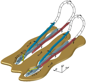


1. Introduction
The near-wall region of wall-bounded flows, composed by the viscous sublayer and the buffer region, is of pragmatic importance for technological applications (Jiménez & Pinelli Reference Jiménez and Pinelli1999). Within this region, flow quantities scale with the friction velocity  $u_{\tau }$ and the viscous unit
 $\delta _{\nu } = \nu /u_{\tau }$, where ν stands for the kinematic viscosity of the fluid. Although\query{Q7} the thickness of the inner region is small compared with the bulk of the flow (Hultmark et al. Reference Hultmark, Vallikivi, Bailey and Smits2012), essential flow features take place, such as the peak of the turbulent kinetic energy production (PR) (Smits, McKeon & Marusic Reference Smits, McKeon and Marusic2011) and a considerable amount of viscous dissipation (DS). Furthermore, a significant fraction of the velocity difference across the mean velocity profile and the skin friction occurs in this region (Jiménez & Moser Reference Jiménez and Moser2007).
To better understand the behaviour of the wall shear stress, its intermittency and its relationship with different flow quantities, a study has been conducted using the large deviation approach of statistical mechanics and conditional averages on turbulent pipe flow direct numerical simulation (DNS) data. Currently, there exist several dispersed studies regarding the flow characteristics associated with backflow events and high wall shear stress events in canonical flows. However, none of those studies reports a complete model indicating the flow features associated with extreme wall-friction events. Hence, in this investigation, we aim to present in detail the near-wall flow features relevant to extreme skin friction events and their relationship with large scales of motion located in the outer region from a statistical point of view. In addition, the present results allow unifying of the findings reported in previous investigations. Finally, we exhibit a conceptual model based on the present statistics, showing the flow structures responsible for the high intermittency in the near-wall region.
Throughout this investigation, the term ‘extreme events’ refers to extreme positive and rare backflow (negative) wall shear stress events, which correspond to the extreme tails of the probability density function of the inner normalised streamwise wall shear stress. A further explanation of the thresholds selected to define these extreme events are found in §§ 2 and 3.
The coordinate system in this study is defined as x in the streamwise direction,  $\theta$ for the azimuthal direction and r for the radial direction. The wall-normal direction is defined as
 $y=R-r$, with
 $R$ being the radius of the pipe. The respective velocities are defined as
 $U_x$,
 $U_\theta$ and
 $U_y = -U_r$ with fluctuating components
 $u_x$,
 $u_\theta$ and
 $u_y = -u_r$. The superscript ‘
 $+$’ is used to denote normalisation in viscous units. The abbreviations EP and BF stand for extreme positive and backflow events throughout this paper. Both abbreviations are also used as a subscript to express conditional averages considering extreme positive or backflow events (e.g.
 $\langle \cdot \rangle _{EP}$ denotes a conditional average for extreme positive events).
1.1. The near-wall intermittent behaviour
The significant magnitudes of flatness of the turbulent velocity components at the viscous sublayer of wall-bounded flows reveal a highly intermittent behaviour (i.e. large deviations). In other words, the high magnitudes of this fourth moment within the viscous sublayer indicate that the probability density function (PDF) has large tails observable several standard deviations from its mean (Farazmand & Sapsis Reference Farazmand and Sapsis2017), which is a mark related to the occurrence of extreme events (Lenaers et al. Reference Lenaers, Li, Brethouwer, Schlatter and Örlü2012; Diaz-Daniel, Laizet & Vassilicos Reference Diaz-Daniel, Laizet and Vassilicos2017). These large deviations are typical in chaotic systems usually characterised by an exponential decay of the probabilities of large fluctuations (Touchette Reference Touchette2009). According to Blonigan, Farazmand & Sapsis (Reference Blonigan, Farazmand and Sapsis2019), large deviations or extreme events in turbulent wall-bounded flows are the result of persistent nonlinear energy transfers and extreme bursts associated with a transmission of energy from large scales of motion (LSM) to the mean flow, producing growth on the energy input and its dissipation rate (Farazmand & Sapsis Reference Farazmand and Sapsis2017).
Several authors have analysed the structures responsible for the high intermittency in near-wall turbulence. A series of numerical experiments (DNS) on wall-bounded flows showed that alternating streamwise velocity streaks together with quasi-streamwise vortices is one of the most important mechanisms to sustain turbulence and hence the near-wall intermittent behaviour (Kim, Moin & Moser Reference Kim, Moin and Moser1987; Robinson Reference Robinson1991; Jiménez & Pinelli Reference Jiménez and Pinelli1999; Schoppa & Hussain Reference Schoppa and Hussain2002). At the outer layers, it is known that there exist large- and very-large-scales of motion (VLSM) that influence the near-wall small scales. Experiments conducted in wall-bounded flows have shown that there are uniform zones of streamwise momentum that scale with the boundary layer thickness (Meinhart & Adrian Reference Meinhart and Adrian1995) or the pipe radius (Kim & Adrian Reference Kim and Adrian1999), and are associated with the existence of packets of aligned hairpin vortices (Kim & Adrian Reference Kim and Adrian1999; Adrian, Meinhart & Tomkins Reference Adrian, Meinhart and Tomkins2000; Adrian Reference Adrian2007). By investigating a relationship between very large scales of motion and the wall shear stress behaviour in wall-bounded flows, Abe, Kawamura & Choi (Reference Abe, Kawamura and Choi2004) analysed data collected from channel flow DNS. The results from that investigation revealed that there exist local peaks of the power spectra of the wall shear stress components located at low wavenumbers whose magnitudes increase with the friction Reynolds number  $\textit{Re}_{\tau}$, revealing that large-scale structures influence the near-wall behaviour and this effect is Re-dependent.
Further investigations revealed how VLSM influence the near-wall dynamics and its intermittency. Hutchins & Marusic (Reference Hutchins and Marusic2007b) collected experimental data using hot-wire probes in turbulent boundary layers (TBL) and observed that LSM and VLSM not only superimpose on the near-wall activity as a low wavenumber mean shift, but they also modulate the amplitude of the near-wall cycle as the envelope of a fluctuating signal (Hutchins & Marusic Reference Hutchins and Marusic2007a,Reference Hutchins and Marusicb; Marusic, Mathis & Hutchins Reference Marusic, Mathis and Hutchins2010). Similarly, Örlü & Schlatter (Reference Örlü and Schlatter2011), using DNS data for turbulent boundary layers, proved that the  $\textit{Re}_{\tau}$ dependency in the root-mean-square of the streamwise wall shear stress fluctuations
 $(\tau _{x,rms}^+)$ is the result of an amplitude modulation effect imposed by LSM and VLSM on the near-wall dynamics.
In practical terms, the energy cost of transportation systems (e.g. pumping losses in pipelines, drag around bodies or sediment transport) is directly related to the behaviour of the mean wall shear stress and its intermittency. Hence, a deeper understanding of the transport phenomena existing close to the wall (Chin et al. Reference Chin, Vinuesa, Örlü, Cardesa, Noorani, Schlatter and Chong2018a) can provide useful insights for important applications such as improvements of drag control techniques (Jiménez & Moser Reference Jiménez and Moser2007), heat and mass transfer enhancement (Marusic et al. Reference Marusic, Mathis and Hutchins2010) and sediment transport (Nelson et al. Reference Nelson, Shreve, McLean and Drake1995; Keshavarzy & Ball Reference Keshavarzy and Ball1999; Lelouvetel et al. Reference Lelouvetel, Bigillon, Doppler, Vinkovic and Champagne2009; Cameron, Nikora & Witz Reference Cameron, Nikora and Witz2020).
1.2. Extreme positive wall shear stress
The velocity structures related to high and extremely high wall shear stress events have been examined using experimental (Sheng, Malkiel & Katz Reference Sheng, Malkiel and Katz2009; Hutchins et al. Reference Hutchins, Monty, Ganapathisubramani, Ng and Marusic2011; Gomit, De Kat & Ganapathisubramani Reference Gomit, De Kat and Ganapathisubramani2018) and DNS (Pan & Kwon Reference Pan and Kwon2018) data for turbulent boundary layers (external flows). Sheng et al. (Reference Sheng, Malkiel and Katz2009) collected three-dimensional data at high resolution by using digital holographic microscopy on a TBL and characterised the different buffer layer vortical structures associated with high and low values of wall shear stress. That study showed that single and paired streamwise vortices related to sweep events with an occurrence of 47 % are related to regions with high magnitudes of wall shear stress. Similarly, the same study revealed that paired streamwise vortices and hairpin-like structures in the inner layer that generate ejection events with an approximate occurrence of 16 % and 2 % respectively are responsible for the existence of regions with low skin friction. Unfortunately, the small size of the instantaneous velocity fields of the investigation mentioned above did not allow us to infer the relationship of the buffer vortices and LSM. Subsequently, Hutchins et al. (Reference Hutchins, Monty, Ganapathisubramani, Ng and Marusic2011) used data, obtained by hot-film shear stress sensors together with hot-wire probes, conditioned under positive and negative skin friction fluctuations (without any thresholds) and revealed that positive and negative wall-friction regions might be the footprint of VLSM located at the logarithmic layer. Similarly, Gomit et al. (Reference Gomit, De Kat and Ganapathisubramani2018) collected data of TBL by particle image velocimetry techniques simultaneously with wall shear stress sensors. That study revealed that the 25 % highest or lowest skin friction fluctuations are related to 75 % deficit or surplus of the streamwise velocity fluctuations. The same investigation also reported that extreme events provide different contributions to the Reynolds shear stress. Taking advantage of the high resolution provided by TBL DNS data sets, Pan & Kwon (Reference Pan and Kwon2018) analysed the flow topology of extreme skin friction events defined as  $|u_\tau ^{\prime }|/u_{\tau ,rms} \geq 4$. That study revealed that extreme positive (EP) events are embedded within large-scale high-speed streaks associated with intense Q4 (sweep) events (regions where
 $u_x > 0$ and
 $u_y < 0$). Additionally, the same investigation asserts that ‘the origin of the strong Q4 events, their Re-dependency and the related spanwise wall shear stress fluctuation features deserve to be further studied’. Similar assertions have been previously stated by other authors (Smits & Marusic Reference Smits and Marusic2013; Hutchins et al. Reference Hutchins, Monty, Ganapathisubramani, Ng and Marusic2011) who highlight the importance of wall shear stress, its relationship to the near-wall dynamics and the effect of LSM and VLSM on it for drag control purposes.
In the context of sediment transport, it has been shown that regions with high values of wall shear stress located below a sweep (Q4) contribute substantially to particle entrainment (Nelson et al. Reference Nelson, Shreve, McLean and Drake1995; Keshavarzy & Ball Reference Keshavarzy and Ball1999; Lelouvetel et al. Reference Lelouvetel, Bigillon, Doppler, Vinkovic and Champagne2009; Fong, Amili & Coletti Reference Fong, Amili and Coletti2019; Cameron et al. Reference Cameron, Nikora and Witz2020) because these structures are more common near the wall compared to other events. Interestingly, the results reported by the studies mentioned above have similarities to the study mentioned earlier, by Pan & Kwon (Reference Pan and Kwon2018), who analysed the velocity structures related to extremely high wall shear stress. Hence, the understanding of the dynamics associated with extremely high skin friction events might be essential for drag control as well as for other practical purposes such as sediment and particle transport. However, to the knowledge of the present authors, there are limited studies about extreme positive wall shear stress events and the flow dynamics involved with them.
1.3. Rare backflow events
Although intuition and results from early experiments might dictate the non-existence of backflow (BF) events in wall-bounded flows (Eckelmann Reference Eckelmann1974), recent experimental (Brücker Reference Brücker2015; Willert et al. Reference Willert, Cuvier, Foucaut, Klinner, Stanislas, Laval, Srinath, Soria, Amili and Atkinson2018) and DNS investigations have shown evidence of regions with negative streamwise velocity within the viscous sublayer (Jalalabadi & Sung Reference Jalalabadi and Sung2018). Other studies have even found reverse flow events at the buffer region (Lenaers et al. Reference Lenaers, Li, Brethouwer, Schlatter and Örlü2012; Cardesa et al. Reference Cardesa, Monty, Soria and Chong2019). After analysing the PDF of the streamwise wall shear stress for TBL DNS data, Örlü & Schlatter (Reference Örlü and Schlatter2011) revealed that the contribution of BF events to the total streamwise wall shear stress  $\tau _x^+$ is less than 0.1 %. Similarly, Lenaers et al. (Reference Lenaers, Li, Brethouwer, Schlatter and Örlü2012) conducted an extensive investigation of backflow events in channel flows, showing that reverse
 $\tau _x^+$ has, on average, a circular shape with an approximate diameter of 20 wall units which are a consequence of an oblique vortex located at the buffer. That oblique vortex seems to be related to layered sweep (Q4) and ejection events (Q2) (Jalalabadi & Sung Reference Jalalabadi and Sung2018).
More recently, Cardesa et al. (Reference Cardesa, Monty, Soria and Chong2019) examined the dynamics of backflow events in turbulent channel flows using conditional averages of volumetric time series. Interestingly, that study revealed a region with significant magnitudes of spanwise vorticity, which has a long streamwise extension associated with backflow events. As a result, they educed a relationship between BF and large-scale events. However, that investigation does not provide further details about the large-scale structures related to BF events.
In addition to canonical flows, Chin et al. (Reference Chin, Vinuesa, Örlü, Cardesa, Noorani, Schlatter and Chong2018a) studied the flow topology of backflow in toroidal pipes. That research revealed that BF events in toroidal pipes have a smaller diameter when compared to channels, and these events are less frequent in the former due to the existence of secondary flows. Bross, Fuchs & Kähler (Reference Bross, Fuchs and Kähler2019) used detailed particle tracking velocimetry to investigate an adverse pressure gradient turbulent boundary layer (APG-TBL), where it was revealed that backflow events located at the viscous sublayer are embedded within low-momentum regions that extend from the wall up to the overlap layer. That investigation also argues that oblique or spanwise vortices have to interact with the low-momentum regions to generate reverse flow events. Another recent study conducted by Wu, Cruickshank & Ghaemi (Reference Wu, Cruickshank and Ghaemi2020) for transitional flat-plate TBL and pipe flows at low  $\textit {Re}_{\tau}$, showed that backflow events are caused by a reverse hairpin vortex, whose circulation is responsible for the presence of an instantaneous BF. However, that investigation does not focus on the near-wall large-scale structures related to negative skin friction events.
Although several studies have unravelled several flow features related to BF events, a complete picture of the mechanisms and large-scale coherent motions responsible for these rare events remains unclear. Hence, conditional analysis from spatial flow realisations of pipe flow DNS is used in this paper to complement the understanding of the coherent structures underlying the highly intermittent behaviour (extreme events) existing at the near-wall region in turbulent wall-bounded flows.
1.4. Aim of this study
Turbulent pipe flow DNS data sets at different Reynolds numbers are used to conduct an investigation into the high intermittency (extreme events) of the wall shear stress vector field and its relationship to different flow quantities. This work aims to provide a comprehensive view of the flow dynamics underlying backflow and extreme positive events, its relationship to the outer large scales of motion and its contribution to flow quantities such as the turbulent inertia, turbulence production and viscous dissipation. This paper is organised as follows: in § 2 we summarise the computational parameters used to conduct the numerical simulations. Wall shear stress statistics and large deviations are analysed in § 3, where empirical relationships are obtained to predict the percentage of extreme events and  $\tau _{rms}^+$ as a function of
 $\textit{Re}_{\tau}$. In § 4 volumetric conditional averages of the wall shear stress components, velocity fluctuations, vorticity and velocity–vorticity correlations are computed using a new scheme that considers the location of the vortex related to EP and BF events. In addition, conditional averages for the production (PR) and dissipation (DS) terms of the balance equations of the Reynolds stress components are presented in § 5, where it is observed that extreme events are also related to high rates of turbulence production and viscous dissipation. A three-dimensional analysis of the near-wall coherent structures responsible for extreme events is presented in § 6. Finally, the conclusions obtained from this study are presented in § 7.
2. Computational approach
The governing equations that describe the motion of a Newtonian incompressible fluid are the Navier–Stokes equations given by
 \begin{gather} \boldsymbol{\nabla} \boldsymbol{\cdot} \boldsymbol{u} = 0, \end{gather}
 \begin{gather}\frac{\partial \boldsymbol{u}}{\partial t} + (\boldsymbol{u}\boldsymbol{\cdot}\boldsymbol{\nabla} )\boldsymbol{\cdot} \boldsymbol{u} = - \boldsymbol{\nabla} p + \frac{1}{Re} \nabla^{2} \boldsymbol{u} + \boldsymbol{f}, \end{gather}
where  $\boldsymbol {u}$ represents the velocity vector field,
 $p$ the pressure scalar field and
 $\boldsymbol {f}$ is a forcing term.
The spatial discretisation for the low friction Reynolds number cases  $\textit {Re}_{\tau} \approx 170$ and
 $500$ is implemented using the spectral element method solver Nek5000 (see Fischer, Kruse & Loth Reference Fischer, Kruse and Loth2002). Seventh-order Lagrangian interpolants on Gauss–Lobatto–Legendre (GLL) quadrature points are the basis of the velocity and pressure spectral mesh. The solver has two main algorithms to resolve the Navier–Stokes equations named
 $P_N P_N$ and
 $P_N P_{N-2}$ (Offermans et al. Reference Offermans, Marin, Schanen, Gong, Fischer and Schlatter2016; Fischer et al. Reference Fischer, Kruse and Loth2002). The former is suitable for solenoidal and non-divergence free flows. Hence, to preserve generality, the
 $P_{N}P_{N}$ solver is used. The temporal integration of the momentum equation was implemented by a third-order backward difference scheme.
For the higher Reynolds number cases  $\textit {Re}_{\tau} \approx 1000$ and 2000, volumetric flow realisations from Chin (Reference Chin2011), Chin, Monty & Ooi (Reference Chin, Monty and Ooi2014a) and Chin et al. (Reference Chin, Philip, Klewicki, Ooi and Marusic2014b) are used. Those numerical simulations are based on a spectral element/Fourier spatial discretisation using eleventh-order GLL points at each spectral element. Additionally, the temporal integration is performed by applying a second-order velocity-correction projection scheme (Blackburn & Sherwin Reference Blackburn and Sherwin2004).
All numerical solutions were conducted on a Cartesian mesh which was later spectrally interpolated over a cylindrical mesh equispaced in the streamwise and azimuthal directions, and Chebyshev in the wall-normal direction. This approach eases the analysis of the canonical turbulent pipe flow due to its cylindrical nature. For the cases studied in this paper, a periodic domain with a length of  $8{\rm \pi} R$ was selected, except for the
 $Re_\tau \approx 2000$ case, where the streamwise extension was
 $3{\rm \pi} R$. In the study by Chin et al. (Reference Chin, Ooi, Marusic and Blackburn2010), they reported that periodicity effects on high-order statistics are negligible when the domain length is at least
 $L_x = 8{\rm \pi} R$. Hence, the data from the
 $Re_\tau \approx 1000$ case are chosen to perform the analysis in this paper.
It is also important to mention that all the simulations ran for at least five turnovers ( $TU_b/Lx$) before gathering data. This prevents any influence of the initial perturbations for each flow field (Chin Reference Chin2011). Subsequently, all the present flow fields ran for at least six turnovers to collect statistics. In addition, the flow realisations used in this investigation have a time span large enough to ensure that each flow field is independent of every other. The main simulation parameters, the grid resolution and the number of independent fields used from each numerical simulation are briefly summarised in table 1.
Computational parameters used in the numerical simulations. The quantity  $TU_b/Lx$ shows the number of turnovers along the flow domain with a streamwise length
 $Lx$ at the bulk velocity
 $U_b$ for a period of time
 $T$.
 $N_F$ stands for the number of independent volumetric flow fields used to compute the present statistics.

To analyse the flow statistics related to extreme events, conditional averages are computed on a box with a size  $-600 \leq {\rm \Delta} _x^+ \leq 1200$,
 $-200 \leq {\rm \Delta} R\theta ^+ \leq 200$ and
 $0 \leq {\rm \Delta} y^+ \leq 500$. The coordinate
 $(0,0,0)$ within the averaging box corresponds to the centroid of the extreme event. This particular box size has been selected to analyse the influence of different flow features occurring upstream and downstream of the extreme events. Additionally, the large box size used in this investigation allows us to examine the outer LSMs associated with the near-wall dynamics of both extreme events studied herein. As expected, the condition used to define a backflow event is
 $\tau _{x}^+ < 0$, where
 $\tau _{x}^+$ denotes the wall shear stress in the streamwise direction normalised in viscous units. On the other hand, the authors have not found a consensus on the thresholds that define extreme positive or extremely high wall shear stress events in the existing literature; hence, the condition used to define extremely high events herein is taken as
 $\tau _{x}^+ > 3.1$. The cutoff value of
 $\tau _{x}^+ > 3.1$ is selected since it provides a similar probability of occurrence for extreme positive events as for backflow events at
 $Re_\tau \approx 1000$, which is the case used to obtain conditional flow fields, as observed in figure 2(a) and table 2. The method used to compute conditional averages is discussed in detail in § 4.
Wall shear stress statistics as a function of  $Re_\tau$.
 $N_{BF}$ and
 $N_{EP}$ stand for the number backflow and extreme positive events (samples) found for the totality of independent fields analysed in each case.

3. Wall shear stress statistics
3.1. Effects of  $\textit {Re}_{\tau}$ on wall shear stress fluctuations

The PDF of the streamwise wall shear stress  $\tau _{x}$ for different Reynolds numbers is shown as solid lines in figure 1(a). The width increment of the tails at different
 $\textit {Re}_{\tau}$ shows a clear influence of the Reynolds number on the occurrence of both extremely positive and backflow events. These results show good agreement with the findings reported by Lenaers et al. (Reference Lenaers, Li, Brethouwer, Schlatter and Örlü2012) for channel flows at
 $\textit {Re}_{\tau} = 180$, 590 and 1000 represented by (
 $\times$) symbols. The vertical dashed lines in figure 1(a) indicate the thresholds used to define the tails of the PDF as defined in § 2. In figure 1(a,b), an exponential decay on the tails is observed, which is an expected behaviour of systems where large deviations exist (Touchette Reference Touchette2009). Although the central region of the PDF, close to the peak, can be modelled using the central limit theorem, the behaviour of the extreme tails can be more precisely analysed using the large deviation theory (Majumdar & Schehr Reference Majumdar and Schehr2017). The work by Diaz-Daniel et al. (Reference Diaz-Daniel, Laizet and Vassilicos2017) proved that a log-normal distribution fits the central region of the probability distribution for the streamwise wall shear stress. However, the log-normal distribution is not suitable to fit the extreme tails. Here, we propose a combined distribution for the streamwise wall shear stress considering a truncated log-normal fit in the range
 $0 \leq \tau _x^+ \leq 3.1$, and an asymmetric double exponential fit for the extreme tails. The results of the exponential fits are plotted in figure 1(a) using the (
 $\Box$) symbol. The function used to fit the left tail of the streamwise wall shear stress PDF in terms of
 $\textit {Re}_{\tau}$ has the form
 \begin{equation} P(\tau_x^+)_{BF} = \xi_{BF} \exp{(\phi_{BF} \tau_x^+\exp{(\psi_{BF}}\tau_x^+))}, \end{equation}
where the coefficients  $\xi _{BF}$,
 $\phi _{BF}$ and
 $\psi _{BF}$ are functions of the Reynolds number as follows
 \begin{gather} \xi_{BF} = -0.0053+0.0011 \ln{(\textit{Re}_{\tau})}, \end{gather}
 \begin{gather}1/\phi_{BF} = 0.114+0.018\ln{(\textit{Re}_{\tau})}, \end{gather}
 \begin{gather}\psi_{BF} = -0.153+0.040\ln{(\textit{Re}_{\tau})}. \end{gather}
Similarly, the right tail for extreme events follows the correlation
 \begin{equation} P(\tau_x^+)_{EP} = \xi_{EP} \exp{(\phi_{EP} \tau_x^+\exp{(\psi_{EP}}\tau_x^+))}, \end{equation}
with coefficients
 \begin{gather} 1/\xi_{EP} = -0.059+0.012\ln{(\textit{Re}_{\tau})}, \end{gather}
 \begin{gather}1/\phi_{EP} = -0.034 - 0.040\ln{(\textit{Re}_{\tau})}, \end{gather}
 \begin{gather}\psi_{EP} = 0.034-0.0064\ln{(\textit{Re}_{\tau})}. \end{gather}
(a) Probability density function of the streamwise wall shear stress  $\tau _{x}^+$ for different
 $\textit{Re}_{\tau}$: (solid line) present results, where (green)
 $\textit {Re}_{\tau} \approx 170$, (red)
 $\textit {Re}_{\tau} \approx 500$, (black)
 $\textit {Re}_{\tau} \approx 1000$, (blue)
 $\textit {Re}_{\tau} \approx 2000$; (
 $\times$) channel flow results from (Lenaers et al. Reference Lenaers, Li, Brethouwer, Schlatter and Örlü2012) at
 $\textit {Re}_{\tau} = 180$, 590 and 1000; (
 $\Box$) correlation presented in (3.1) and (3.5). The dashed lines are the cutoff conditions used to define the extreme events. The arrow represents an increment in
 $\textit{Re}_{\tau}$. (b) Probability density function of the azimuthal wall shear stress
 $\tau _{x}^+$ for the present results.

The PDF of the azimuthal  $\tau _{\theta }^+$ fluctuations for different Reynolds numbers is observed in figure 1(b) where a similar behaviour is observed in terms of
 $\textit{Re}_{\tau}$, with symmetric exponential behaviour at the tails. A symmetric behaviour is also found in the full conditional averages of
 $\tau _\theta ^+$ for both EP and BF events, as will be discussed later.
Although the contribution of the extreme tails of the  $\tau _x^+$ PDF is less than 0.2 % when compared with the total contribution of the most probable events (close to the peak of the distributions), the understanding of the dynamics related to EP and BF events can provide useful insights for drag control purposes since it contributes importantly to the deficit or surplus of the components of the Reynolds stress tensor (Gomit et al. Reference Gomit, De Kat and Ganapathisubramani2018). Consequently, extreme events are related to high magnitudes of turbulent kinetic energy production and viscous dissipation, as analysed and presented in § 5.
The percentage of extreme events at different  $\textit {Re}_{\tau}$ in terms of the thresholds used in this work is shown in figure 2(a). The present results for BF events at different Reynolds numbers ranging from
 $\textit {Re}_{\tau} \approx 170$ up to
 $2000$ are represented by (
 $\Diamond$). Our data have been compared with the studies conducted by Lenaers et al. (Reference Lenaers, Li, Brethouwer, Schlatter and Örlü2012) and Hu, Morfey & Sandham (Reference Hu, Morfey and Sandham2006) for channel flows, showing good agreement. It is also interesting to notice that the percentage of BF events increases as a logarithmic correlation of the form
 \begin{equation} \% {BF} = -0.147 + 0.031 \ln{(\textit{Re}_{\tau})}.\end{equation}
(a) Per cent of backflow events at the wall; ( $\Diamond$) present, (
 $\times$) channel flow by Lenaers et al. (Reference Lenaers, Li, Brethouwer, Schlatter and Örlü2012), (
 $\triangle$) channel flow by Hu et al. (Reference Hu, Morfey and Sandham2006), (solid) correlation of the form
 $\% {BF} = -0.147 + 0.031 \ln {(\textit{Re}_{\tau})}$. The red symbols represent EP events being (
 $\circ$) present, and (
 $\dotsm$) linear correlation
 $\%\textit {EP}=7.2\times 10^{-5} \textit {Re}_{\tau}+0.0019$. (b) Root mean square of wall shear stress fluctuations; (
 $\Diamond$) present, (
 $+$) pipe flow by El Khoury et al. (Reference El Khoury, Schlatter, Brethouwer and Johansson2014), (
 $\triangle$) channel flow by Hu et al. (Reference Hu, Morfey and Sandham2006), (
 $---$) correlation by Schlatter & Örlü (Reference Schlatter and Örlü2010) for
 $\tau _{x,rms}^+$ in TBL, (
 $-\cdot -$) correlation by Diaz-Daniel et al. (Reference Diaz-Daniel, Laizet and Vassilicos2017) for
 $\tau _{\theta ,rms}^+$ in TBL, (solid lines) correlation of the form
 $\tau _{rms}^+ = a + 0.0355 \ln {(\textit {Re}_{\tau})}$ where
 $a=0.168$ for the streamwise component and
 $a=0.025$ for the azimuthal component.

Likewise, the percentage of extreme positive events (%EP) is represented by ( $\circ$) in figure 2(a) and seems to follow a linear behaviour for the selected threshold. Therefore, the cutoff
 $\tau _x^+ > 3.1$ used to characterise the extreme positive events seems to be suitable at
 $Re_\tau \leq 1000$ since this value is related to the same contributions of EP and BF to the probability distribution of
 $\tau _x^+$ (see table 2). However, at higher Reynolds numbers, a different value for the threshold might be required to be used to define the EP events.
The value of the normalised root-mean-square of the wall shear stress fluctuations ( $\tau _{x,rms}^+$ and
 $\tau _{\theta ,rms}^+$) has been plotted in figure 2(b). Data from the present study, El Khoury et al. (Reference El Khoury, Schlatter, Brethouwer and Johansson2014) for pipe and Hu et al. (Reference Hu, Morfey and Sandham2006) for channel flows are displayed. The dashed lines represent the correlations proposed by Schlatter & Örlü (Reference Schlatter and Örlü2010) and Diaz-Daniel et al. (Reference Diaz-Daniel, Laizet and Vassilicos2017) for the streamwise and the spanwise wall shear stress fluctuations in TBL, respectively. The
 $\tau _{rms}^+$ for internal flows (channel and pipe) agrees with the boundary layer correlations at high Reynolds numbers. However, at low
 $\textit {Re}_{\tau}$, the trend of
 $\tau ^+_{rms}$ seems to follow a different correlation with respect to the TBL correlations. The differences found between internal and external flows at low
 $\textit {Re}_{\tau}$ might exist due to the pressure gradient required to drive the flow in internal geometries, as explained by Schlatter & Örlü (Reference Schlatter and Örlü2010). Therefore, for internal flows, the correlation
 \begin{equation} \tau_{rms}^+ = a + 0.0355 \ln{(\textit{Re}_{\tau})}, \end{equation}
is the best fit for the current data, with  $a=0.168$ for the streamwise component and
 $a=0.025$ for the azimuthal component.
The percentage of backflow events in terms of the wall-normal position is shown in figure 3(a). The results are plotted for the pipe flow case at  $\textit {Re}_{\tau} \approx$ 170, 500 and 1000, and exhibit a similar behaviour compared to the channel flow by Lenaers et al. (Reference Lenaers, Li, Brethouwer, Schlatter and Örlü2012). As a complement, figure 3(b) presents the outermost location at which backflow events of the streamwise velocity fields
 $U_x$ are found. Interestingly, at the lowest Reynolds number studied, it is observed that reverse flow events occur within the viscous sublayer. In contrast, at the higher Reynolds numbers
 $\textit {Re}_{\tau} \geq 1000$, it is possible to observe backflow events at the buffer region.
(a) Percentage of backflow events as a function of the wall-normal location for  $\textit {Re}_{\tau} \approx 170$, 500 and 1000; (
 $\times$) channel flow by Lenaers et al. (Reference Lenaers, Li, Brethouwer, Schlatter and Örlü2012). The arrow represents increment in
 $\textit{Re}_{\tau}$. (b) Outermost location of backflow events as a function of
 $\textit{Re}_{\tau}$; (
 $\Diamond$) present results, (
 $\times$) Lenaers et al. (Reference Lenaers, Li, Brethouwer, Schlatter and Örlü2012) and (
 $\Box$) Jalalabadi & Sung (Reference Jalalabadi and Sung2018), (
 $---$) limit of the viscous sublayer.

4. Flow statistics under extreme events
Next, we analyse flow statistics and display conditional averages computed only for the pipe flow case at  $\textit {Re}_{\tau} \approx 1000$. The authors also examined flow averages from the lower Reynolds number data. Since the results of the conditional fields are invariant within the Reynolds number range studied, agreeing with Cardesa et al. (Reference Cardesa, Monty, Soria and Chong2014), the
 $\textit {Re}_{\tau} \approx 1000$ data are presented in this study. The number of backflow and extreme positive skin friction events used to compute the present conditional fields at
 $\textit {Re}_{\tau} \approx 1000$ are 7791 and 6573 respectively. This number of samples allow us to obtain convergent flow statistics.
4.1. Conditional average scheme
Volumetric conditional fields have been computed to study the different flow quantities related to extreme events. It is important to note that conditional averages based solely on a single condition (e.g.  $\tau _x^+ < 0$), usually lead to symmetric results. Indeed, this problem has already been observed and discussed by Sheng et al. (Reference Sheng, Malkiel and Katz2009). Turbulent structures are seldom symmetric. It is reported that low-velocity structures are characterised by their meandering behaviour (see Hutchins et al. (Reference Hutchins, Monty, Ganapathisubramani, Ng and Marusic2011) or Jiménez (Reference Jiménez2018)). Furthermore, observing symmetrical vortical structures at the near-wall region at high
 $\textit {Re}_{\tau}$ is unlikely (Robinson Reference Robinson1991; Schoppa & Hussain Reference Schoppa and Hussain2002; Adrian Reference Adrian2007). Hence, it is difficult to capture meaningful kinematics of the fluid motion by conducting conditional averages based only on the EP or BF wall shear stress events using a single threshold. Thus, in this investigation, we have implemented a two-step conditional average considering the following conditions, as illustrated in figure 4:
(i) The centroid of the extreme event on the two-dimensional streamwise wall shear stress field is located in terms of the thresholds proposed in § 3. An averaging box is used, with size
${\rm \Delta} x^+=1800$ in the streamwise direction, ${\rm \Delta} R\theta ^+=400$ in the azimuthal direction and $y^+ = 500$ in the wall-normal direction. The centroid of the extreme event is located within the averaging box at the coordinate ${\rm \Delta} x^+ = 0$, ${\rm \Delta} R\theta ^+ = 0$ and $y^+ = 0$ in the streamwise, azimuthal and wall-normal directions respectively.(ii) After finding the centroid of the extreme event, a second condition is used to detect the presence of a left- (
$Q_L$) or a right-sided ($Q_R$) vortex in terms of the second invariant of the velocity gradient field at the vicinity of the BF or EP event centroid using a smaller secondary box. As a convention, a left-sided vortex will be defined as a vortex located at the left of the box centreline with respect to the flow direction. The opposite condition defines a right-sided vortex for the purposes of this particular research (see figure 4 for clarity).


Scheme used to compute conditional averages.

A similar approach has been used previously by Lenaers et al. (Reference Lenaers, Li, Brethouwer, Schlatter and Örlü2012), who observed that BF events are related to the existence of an oblique vortex. Likewise, Hutchins et al. (Reference Hutchins, Monty, Ganapathisubramani, Ng and Marusic2011) used a comparable method based on the values of the friction velocity for four points at the vicinity of a negative event in order to characterise the meandering behaviour of low-speed streaks in turbulent boundary layers. This approach has been proven to detect relevant flow features, as will discussed in the following sections.
4.2. Conditional wall shear stresses
Figures 5(a) and 5(d) exhibit the conditional average of  $\tau _x^+$ under the effect of a conditionally averaged left-sided vortex (hereinafter
 $Q_L$) for EP and BF events, respectively. As observed, when the aforementioned scheme is used, the averaged quantities are not symmetrical with respect to the streamwise centreline. Similar results, but under the effect of a right-sided vortex (
 $Q_R$) are also displayed in figures 5(b) and 5(e). Conversely, when conditional averages do not discriminate the location of the vortices, symmetrical results are obtained, as observed on figures 5(c) and 5(f). More substantial differences when using the proposed scheme are observed when figures 6(d) and 6(e) are compared with figure 6(f), where the footprint of the oblique vortex responsible for the BF events is clearly observed in the two-step conditioned fields.
Contours represent conditional ensemble averages of  $\tau _x^+$ conditioned to EP events (a–c) and BF events (d–f). The extreme event centroid is located at
 ${\rm \Delta} x^+=0$ and
 ${\rm \Delta} R\theta ^+=0$. (a,d) Under the effects of a left-sided structure (dark isosurface). (b,e) Ensemble averages considering a right-sided structure. (c,f) Full conditional averages (without the consideration of the structure orientation). The dark isosurfaces in all figures are conditional
 $Q$ vortical structures at a level
 $Q^+=0.5$.

Conditional averages of  $\tau _{\theta }^+$ conditioned to EP events (a–c) and BF events (d–f). Averages have been computed under the same conditions as figure 5.

4.2.1. Streamwise wall shear stress
It can be noticed in figure 5(a) that the extreme positive wall shear stress event, presented as a colour contour, has a slightly oblique elliptical shape, tilted towards the orientation of the quasi-streamwise vortex related to it (in a darker colour). The topology of the streamwise vortex associated with high wall friction is in good agreement with the results reported by Kravchenko, Choi & Moin (Reference Kravchenko, Choi and Moin1993) and Sheng et al. (Reference Sheng, Malkiel and Katz2009).
The white contour line in figure 5(c) shows the threshold used in this study to characterise EP events  $(\tau _x^+>3.1)$, which has an approximate size of
 $30\times 10$ wall units on its major and minor axes, respectively. The EP
 $\tau _x^+$ event is associated with a quasi-streamwise vortex which transports streamwise momentum from the overlap and outer layers towards the wall. Then, a region of high streamwise momentum located at the viscous sublayer and the buffer is engendered, producing a large streamwise velocity gradient. Consequently, it is educed that the EP wall shear stress is the footprint of a high-momentum region created by a quasi-streamwise vortex, as explained further in § 4.3.
Although the features observed from conditional backflow wall shear stress fields resemble the results obtained by Chin et al. (Reference Chin, Vinuesa, Örlü, Cardesa, Noorani, Schlatter and Chong2018a) and Cardesa et al. (Reference Cardesa, Monty, Soria and Chong2014), figure 5(d), related to a left-sided vortex, unveils a non-symmetric shape of the conditioned  $\langle \tau _x^+ \rangle _{BF}$ field with respect to the streamwise axis of the averaging box. Unlike EP events, here, the reverse flow is caused by an oblique vortex, responsible for the generation of negative velocity gradients at the near-wall region, which agrees with the vortical structure reported by Lenaers et al. (Reference Lenaers, Li, Brethouwer, Schlatter and Örlü2012). Figure 5(f) shows the full conditional average of
 $\langle \tau _x^+ \rangle _{BF}$ with its associated
 $Q$ conditional structure. Here, the
 $Q$ structure exhibits a similar topology to the conditional inverted hairpin vortex first shown by Chin et al. (Reference Chin, Monty, Chong and Marusic2018b) for critical points and also observed by Wu et al. (Reference Wu, Cruickshank and Ghaemi2020), for negative skin friction in transitional flows. Although this structure might resemble a reverse hairpin vortex, our instantaneous visualisations of
 $Q$ show that, at high
 $Re$, oblique or spanwise vortices are more likely to occur, which agrees with the buffer structures reported by Sheng et al. (Reference Sheng, Malkiel and Katz2009), Lenaers et al. (Reference Lenaers, Li, Brethouwer, Schlatter and Örlü2012) and Bross et al. (Reference Bross, Fuchs and Kähler2019) for zero-pressure-gradient turbulent boundary layer (ZPG-TBL), channel flows and APG-TBL respectively. The oblique vortex identified in this investigation is not in disagreement to the inverted vortex observed by Wu et al. (Reference Wu, Cruickshank and Ghaemi2020) since their study was conducted for transitional flows at low
 $Re$, where inverted hairpins are more likely to occur. Indeed, our full conditioned
 $Q$ structure at
 $\textit {Re}_{\tau} \approx 1000$ (see figure 5f) has the same topology as the conditional
 $\lambda _{ci}$ structure revealed by Wu et al. (Reference Wu, Cruickshank and Ghaemi2020) on transitional flows at low and moderate
 $\textit{Re}_{\tau}$. This finding provides further evidence that the near-wall mechanisms responsible for backflow events are Reynolds number independent, and their configuration scale in viscous units.
In terms of large-scale structures, figure 5(d–f) reveals the existence of a region with low values of wall shear stress ( $\tau _x^+ < 1$) located downstream of the negative event with an approximate extension of 300 wall units in the x-direction. That observation is consistent with the large region of positive
 $\langle \omega _\theta \rangle _{BF}$ located downstream of the reverse flow event, which seems to be related to LSMs as identified by Cardesa et al. (Reference Cardesa, Monty, Soria and Chong2019) for channel flows. However, that study does not provide further details, such as the topology, of the LSM responsible for the secondary low
 $\tau _x^+$ region. The elongated low
 $\tau _x^+$ zone is linked to an alternating behaviour of the
 $\tau _\theta ^+$ backflow field (see figure 6d) at the same streamwise locations (
 $50 \leq {\rm \Delta} x^+ \leq 300$). This observation suggests the existence of two large-scale counter-rotating vortical structures that give rise to a low-speed structure. Evidence of the roll modes (i.e. large-scale counter-rotating motions oriented in the streamwise direction) associated with BF events is further examined in the following sections.
4.2.2. Azimuthal wall shear stresses
Even though its ensemble mean value is zero, the azimuthal conditioned wall shear stress fields provide useful information of the vortical structures oriented in the streamwise direction that lie above the events analysed. The  $\tau _\theta ^+$ conditional averages observed in figure 6 have been computed under the same conditions as the
 $\tau _x^+$ fields from figure 5. Figure 6(a) exhibits the azimuthal wall shear stress under the influence of a left-sided quasi-streamwise vortex related to EP events. The positive (red) region has a geometrical shape that resembles the
 $Q_L$ structure which is the result of large azimuthal velocity gradients related to a region of high positive
 $\theta$-momentum generated at the near-wall region. Although non-symmetrical, but similar in shape, figure 6(a) evinces a pair
 $\tau _\theta ^+$ with opposite sign also due to the increment of momentum in the viscous sublayer and the buffer but in the negative
 $\theta$ direction. The analysis of the velocity fields examined in § 4.3 provides a clearer view of the kinematics that originate this behaviour in
 $\langle \tau _\theta ^+ \rangle _{EP}$.
Figure 6(d) displays the  $\tau _\theta ^+$ field conditioned to a backflow event with the presence of a left-sided oblique vortex. Herein, the region with high positive
 $\tau _\theta ^+$ seems to be the footprint of the strong oblique vortex related to the BF event. It is interesting to note the existence of two opposite and symmetric regions along the box centreline located within
 $50 \leq {\rm \Delta} x^+ \leq 300$. That behaviour persists in figure 6(d–f), which proves the influence of large scales of motion in backflow events. In short, the observed results suggest that the BF event is, on average, not only the result of a strong oblique vortex, but it is also related to the existence of a large-scale low-speed streak. The characteristics of the low-speed streak and the mechanisms responsible for BF events are analysed in the following sections.
4.3. Conditional velocity fluctuations
Here, an examination of the three-dimensional velocity structures related to extreme events is presented. Particularly, the focus is on the streamwise and wall-normal turbulent velocity fields. The contour plots are complemented with transverse slices and vector plots which aim to identify the flow dynamics associated with extreme wall shear stress events. It should be mentioned that all the conditional fields presented hereinafter are based on a left-sided ( $Q_L$) vortex unless otherwise stated.
As discussed previously, EP events are related to the existence of a strong quasi-streamwise vortex. Figure 7(a) exhibits the existence of a high streamwise momentum region ( $u_x^+ \geq 4.5$) located at the buffer region between
 $-50 \leq {\rm \Delta} x^+ \leq 150$. This small-scale region of high velocity exists due to the transport of streamwise momentum from the overlap and outer layer towards the wall, induced by the aforementioned vortex, agreeing with the buffer structures associated with high skin friction investigated by Sheng et al. (Reference Sheng, Malkiel and Katz2009). In addition, it is noted that the high-momentum region is embedded within a large-scale structure of positive fluctuation whose streamwise extension scales with the characteristic length of the pipe
 $\delta =R$. This large-scale structure is located at the logarithmic and outer regions, extending up to
 $y^+\approx 400$ or
 $y /\delta \approx 0.4$ in the wall-normal direction.
(a) Ensemble average of streamwise velocity fluctuations conditioned by an EP event on the  ${\rm \Delta} x^+\hbox{--}y^+$ plane at
 ${\rm \Delta} R\theta ^+ = 0$. (b) Transverse sections of (a) at different streamwise locations. (c) Ensemble average of wall-normal velocity fluctuations conditioned by an EP event on the
 ${\rm \Delta} x^+\hbox{--}y^+$ plane at
 ${\rm \Delta} R\theta ^+ = 0$. (d) Transverse sections of (c).

The transverse slices displayed in figure 7(b) at  ${\rm \Delta} x^+=0$ and 100 show that at the left side of the high-momentum region, at the viscous sublayer and the buffer, a low-speed region is created. This structure seems to be a nascent lifted streak with low streamwise momentum. This lifted streak is the result of the transport of momentum from the wall towards the outer layer and is located at the upwash flank of the strong quasi-streamwise vortex. This structure shows coherence, and its topology has similarities to the unstable low-speed streaks related to the near-wall vortex regeneration cycle (Jiménez & Pinelli Reference Jiménez and Pinelli1999; Schoppa & Hussain Reference Schoppa and Hussain2002; Masahito et al. Reference Masahito, Yasufumi, Yuki and Michio2007).
Figures 7(c) and 7(d) show the averaged configuration of the wall-normal velocity ( $u_y^+$) structures related to the EP
 $\tau _x^+$ events under the influence of a
 $Q_L$ vortex. Figure 7(c) shows that there exists a strong region of downwash motion at the inner region associated with the high streamwise momentum region mentioned above. As a result, a strong Q4 layer is created in the viscous sublayer and buffer region just above the EP event, agreeing with the study conducted by Pan & Kwon (Reference Pan and Kwon2018). Additionally, it is observed that, in the logarithmic and outer layers, there exists a large-scale region of negative wall-normal velocity. This provides further evidence that large-scale outer structures are related to the near-wall intermittency. The mechanism related to the existence of these large scales of motion will later be analysed using vector plots (in § 6).
The transverse sections, displayed in figure 7(d), reveal a pair of opposite wall-normal velocity regions located at  $y^+<30$ just above the EP event. These upwash and downwash motions, located at the near-wall region, are produced at both flanks of the quasi-streamwise vortex. It should be noted that the downwash (
 $u_y^+<0$) side is associated with the high streamwise momentum region whereas the upwash side is related to the lifted low-speed streak (see figure 7b), showing the essential role that streamwise vortices have in the near-wall cycle (Robinson Reference Robinson1991; Jiménez & Pinelli Reference Jiménez and Pinelli1999; Schoppa & Hussain Reference Schoppa and Hussain2002). Surprisingly, the high magnitudes of
 $\langle u_y^+ \rangle _{EP}$ and its disposition in pairs resemble the studies conducted by Xu et al. (Reference Xu, Zhang, den Toonder and Nieuwstadt1996) and Lenaers et al. (Reference Lenaers, Li, Brethouwer, Schlatter and Örlü2012). Xu et al. (Reference Xu, Zhang, den Toonder and Nieuwstadt1996), defined the extreme wall-normal events as
 $|u_y / u_{y,rms} | > 5$. Our conditioned values reveal a similar behaviour with negative
 $u_y/u_{y,rms} \approx -7$ and the positive
 $u_y/u_{y,rms} \approx 5$. The work by Xu et al. (Reference Xu, Zhang, den Toonder and Nieuwstadt1996) also mentions that extreme wall-normal events are related to a streamwise vortex located on the buffer layer. Similar observations are laid out by Lenaers et al. (Reference Lenaers, Li, Brethouwer, Schlatter and Örlü2012). However, none of the aforementioned authors studied the relationship of extreme wall-normal velocity with extreme positive
 $\tau _x^+$ events, and the additional coherent outer motions associated with them. As a consequence, our results provide further evidence that streamwise vortices are an essential mechanism to sustain near-wall turbulent energy transfers since they provide large contributions to the total Reynolds shear stress
 $\langle -u_y u_x \rangle ^+$ (not shown here), turbulent kinetic energy production (PR) and viscous dissipation (DS) as will be further analysed in § 5. Finally, it is important to highlight that, if the location of the vortex were not considered with the conditional averages, symmetric results would be observed in figure 7(d) this being a trio of alternating extreme events of wall-normal velocity.
The existence of near-wall strong sweep events related to high skin friction events is more clearly observed at the zoomed view of the streamwise velocity fluctuation field from figure 8, where the vector plots clearly exhibit the interaction of the streamwise vortex and the high- and low-momentum structures associated with EP wall-friction events.
(a) Extended view of figure 7(b) at  ${\rm \Delta} x^+ = 50$, showing the velocity vectors for the
 $u_\theta ^+$ and
 $u_y^+$ components. (b) Zoomed view of streamwise turbulent velocity on a
 ${\rm \Delta} x^+\hbox{--}y^+$ plane sectioned at
 ${\rm \Delta} R \theta^+ = -15$. Vectors represent the conditional velocity fluctuations for
 $u_x^+$ and
 $u_y^+$. The white line contour exhibits the quasi-streamwise vortex.

Similarly, the streamwise velocity fluctuations averaged under negative  $\tau _x^+$ events displayed in figure 9(a,b), exhibit a qualitative behaviour that resembles the results for no-slip critical points (points at the wall where the streamwise and the spanwise skin friction are simultaneously zero) obtained by Cardesa et al. (Reference Cardesa, Monty, Soria and Chong2014) and Chin et al. (Reference Chin, Monty, Chong and Marusic2018b). The present results, in addition, show that the reverse flow event occurs below the tail of a large-scale low-speed streak. It is also interesting to observe that the approach used to compute the conditional averages in this study unveils the average meandering of the low- and high-speed structures as exhibited in the transverse sections shown in figure 9(b). These results are consistent with the existence of the strong oblique vortex that seems to be associated with BF events. In figure 9(a,b) it should also be noted that the low-speed streak associated with BF events is located below a large-scale structure of positive streamwise turbulent fluctuation. This shows that backflows are associated with the interaction of two uniform-momentum zones (UMZ) of low and high momentum, respectively, which generate high shear at their interface. The existence of a large structure of positive
 $u_x^+$ located at the overlap and outer region is in good agreement with the amplitude modulation effect of outer LSM in the near the wall dynamics. These results suggest a different mechanism to the recent study by Bross et al. (Reference Bross, Fuchs and Kähler2019) on APG-TBL who argue that reverse flow events exist below a low-speed superstructure located at the log-law region. These dissimilarities might be due to differences between canonical flows and the large regions with a reverse flow that characterise the velocity profile of an APG-TBL.
(a) Ensemble average of streamwise velocity fluctuations conditioned on BF events on the  ${\rm \Delta} x^+\hbox{--}y^+$ plane at
 ${\rm \Delta} R\theta ^+ = 0$. (b) Transverse sections of (a) at different streamwise locations. (c) Ensemble average of wall-normal velocity fluctuations conditioned under BF events on the
 ${\rm \Delta} x^+\hbox{--}y^+$ plane at
 ${\rm \Delta} R\theta ^+ = 0$. (d) Sections of (c) at different streamwise locations.

Figure 9(c,d) displays the behaviour of BF conditioned wall-normal velocity fluctuations. The existence of positive and negative coherent wall-normal velocity fluctuations on the  ${\rm \Delta} x^+\hbox{--}y^+$ and
 ${\rm \Delta} R\theta ^+\hbox{--}y^+$ planes is consistent with the existence of an oblique vortex. However, the magnitudes of
 $u_y/u_{y,rms}$ are not large enough to assert a relationship between BF events and extreme wall-normal fluctuations. Another interesting observation is that the large-scale low-speed streak in figure 9(a) and the large-scale structures of
 $\langle \tau _x^+ \rangle _{BF}$ and
 $\langle \tau _\theta ^+ \rangle _{BF}$, displayed previously in figures 5 and 6, are related to a long region with positive
 $u_y$ with an approximate streamwise extension of
 $1000$ wall units as observed in the section displayed in figure 9(c). At the logarithmic and outer layers, in the range
 $-200 < {\rm \Delta} x^+ < 500$, we note the presence of a region of negative
 $u_y$, an outer downwash region related to the existence of the large-scale structure of high momentum. This downwash motion can be induced, in part, by the strong oblique vortex. However, the vector plot sections exhibited in § 6 suggest that large-scale rotating motions might also be responsible for the existence of this structure of negative
 $u_y$.
The transverse velocity sections shown in figure 9(d) at  ${\rm \Delta} x^+ = 100$, 200 and 300 reveal that the positive
 $u_y$ region located at the centre of the buffer region is surrounded by negative wall-normal velocity fluctuations on its sides. This behaviour suggests the presence of large streamwise counter-rotating inclined motions which transport momentum from the inner region towards the overlap and outer layers, and hence, those structures are consistent to the existence of the low-speed streak displayed in figure 9(a,b). Further evidence of these swirl motions is provided in § 4.4. As a result, it is educed that backflow events, on average, require the combination of a complex set of fluid motions to occur at the same time (high-velocity LSM at the outer layer, low-speed streaks, an oblique or a spanwise vortex and large-scale counter-rotating motions). Such a combination of complex kinematics makes reverse flow events extremely rare.
To complement the three-dimensional understanding of the averaged small-scale flow dynamics occurring in BF events, figure 10(a,b), respectively, show an expanded view of a transverse and a longitudinal section of the contours for  $\langle u_x^+\rangle _{BF}$ accompanied by the velocity vectors and a line contour of the oblique vortex (white). In figure 10, the centre of the strong vortex and its effects on the high- and low-velocity structures can be clearly observed.
(a) Extended view of figure 9(b) at  ${\rm \Delta} x^+ = 0$ showing the vectors for the
 $u_\theta ^+$ and
 $u_y^+$ components. (b) Zoomed view of streamwise velocity fluctuations on a
 ${\rm \Delta} x^+\hbox{--}y^+$ plane sectioned at
 ${\rm \Delta} R \theta ^+ = 0$ displaying the velocity fluctuation vectors for the
 $u_x^+$ and
 $u_y^+$ components. The white line contour exhibits the oblique vortex at
 $Q^+=0.5$.

4.4. Conditional vorticity
The azimuthal  $\omega _\theta$ and wall-normal
 $\omega _y$ conditional vorticity fields are analysed using a similar approach as in § 4.3 to study the dynamics related to extreme events further.
Extreme positive conditional vorticity fields are shown in figure 11. The azimuthal vorticity component is shown in figure 11(a,b). The conditioned  $\langle \omega _\theta \rangle _{EP}$ volumetric field has been normalised by the ensemble average
 $\langle \omega _\theta \rangle$. This normalisation allows us to observe the regions with surplus or deficit vorticity when compared with the ensemble averaged flow quantities. It is interesting to notice that in the range
 $-50 \leq {\rm \Delta} x^+ \leq 50$ and below
 $y^+=2$ the EP conditioned field exhibits a region with
 $\omega _\theta$ surplus with a similar shape as the conditioned
 $\langle \tau _x^+ \rangle _{EP}$ (see figure 5a). This region with high magnitudes of
 $\omega _\theta$ is created due to the high shear produced due to the presence of a small-scale high-speed streak located above the EP event. Above the viscous sublayer (
 $y^+>5$) and in the range
 $-50 \leq {\rm \Delta} x^+ \leq 200$, there is a region with an azimuthal vorticity deficit, located over the near-wall high streamwise momentum structure observed in figure 8(a).
(a) Value of  $\langle \omega _\theta \rangle _{EP} / \langle \omega _\theta \rangle$ on the
 ${\rm \Delta} x^+\hbox{--}y^+$ plane at
 ${\rm \Delta} R\theta ^+ = 0$. The black vertical dashed lines show the streamwise locations of the transverse sections shown in (b). (c,d) Value of
 $\langle \omega _y^+ \rangle _{EP}$ on the
 ${\rm \Delta} x^+\hbox{--}{\rm \Delta} R\theta ^+$ plane at
 $y^+ \approx 5$ and
 $y^+ \approx 20$ respectively. The
 $\langle \omega _y^+ \rangle _{EP}$ contours are accompanied by turbulent velocity vector plots. (e) Sections of (d).

In figure 11(a), at the location between  $300 < {\rm \Delta} x^+ < 1200$ and
 $70<y^+<200$ there exits an inclined large-scale region with a slight surplus of spanwise vorticity generated below the large-scale structure of positive streamwise fluctuation discussed in the previous section. In contrast, there exists a region with vorticity deficit over the region with vorticity surplus above
 $y^+>200$. These large-scale vorticity layers located downstream from the EP event, exist due to the presence of the shear layers that bound large-scale uniform-momentum zones (UMZ).
Another interesting feature is observed in the transverse sections from figure 11(b), particularly at the transverse sections at  ${\rm \Delta} x^+ = 0$ and 100, where\query{Q23} a small region of high
 $\omega _\theta$ appears at the zone where
 $25<y^+<40$ and
 $10<{\rm \Delta} R\theta ^+<50$ whose centreline is at the interface located between the lifted streak observed in figure 8(a) and the higher-velocity region above it. This finding highlights the importance of lifted streaks in the generation of new vortical structures as suggested by Jiménez & Pinelli (Reference Jiménez and Pinelli1999), Schoppa & Hussain (Reference Schoppa and Hussain2002) and Adrian (Reference Adrian2007).
The wall-normal vorticity component  $\omega _y = -\omega _r$ has also been analysed to understand further the vortical structures related to extreme events. Figure 11(c,d) exhibits wall-parallel sections of
 $\omega _y$ conditioned for EP events taken at
 $y^+\approx 5$ and
 $y^+ \approx 20$ respectively. From the wall-parallel section at
 $y^+ \approx 5$, it should be noticed that the shape of the wall-normal vorticity field resembles the conditional azimuthal wall shear stress field
 $\langle \tau _\theta ^+ \rangle _{EP}$, which suggests its correlation with the quasi-streamwise vortex associated with EP events. Moreover, the transverse sections from figure 11(e) show that
 $\omega _y$ coherent motions are inclined towards the core as
 ${\rm \Delta} x^+$ increases. Hence, it is educed that
 $\tau _\theta$ is the footprint of the vortical motions that occur at the buffer and are inclined towards the pipe centreline. These results provide evidence that coherent quasi-streamwise vortices located at the inner region are responsible for significant contributions to the total drag force. Hence, the strong quasi-streamwise vortex would be an essential structure to analyse in terms of drag control. That information is consistent with the recommendations made by Jiménez & Moser (Reference Jiménez and Moser2007) which advocate focussing on the inner region for drag control purposes and Pan & Kwon (Reference Pan and Kwon2018) who states that EP events and its dynamics should be better understood in the same context.
Figures 12(a) and 12(b), similarly, exhibit the  $\omega _\theta$ field conditioned for backflow events. The
 $\langle \omega _\theta \rangle _{BF} / \langle \omega _\theta \rangle$ field shows the existence of a small region with negative
 $\omega _\theta$ with similar dimensions as the negative
 $\tau _x^+$ event (see figure 5d). The negative
 $\omega _\theta$ region extends up to a wall-normal location
 $y^+ \approx 0.5$. Above the viscous sublayer, there exist two regions with high positive magnitudes of azimuthal vorticity, which are in good agreement with the studies conducted by Cardesa et al. (Reference Cardesa, Monty, Soria and Chong2014) and Cardesa et al. (Reference Cardesa, Monty, Soria and Chong2019). In addition to the studies mentioned above, our conditional averaging method highlights a meandering behaviour of the BF conditioned azimuthal vorticity field observed in the transverse sections taken in figure 12(b). The meandering behaviour of the azimuthal vorticity field is clearly observed in the region of positive
 $\omega _\theta$ located at
 $y^+ > 20$, where its spanwise location is shifted approximately 20 wall units from the averaging box centreline at the transverse section at
 ${\rm \Delta} x^+ = 0$ from figure 12(b). The transverse section at
 ${\rm \Delta} x^+ = 100$ shows that the positive
 $\omega _\theta$ region shifts back to
 $R\theta ^+ = 0$. These coherent structure with high magnitudes of
 $\omega _\theta$ are the result of the interaction between the lifted low-speed streak and the large-scale high-velocity structure located above it (see figure 9a). Consequently, the coherent
 $\omega _\theta$ region seems to have a streamwise extension akin to the averaged low-speed streak associated with BF events.
(a) Value of  $\langle \omega _\theta \rangle _{BF} / \langle \omega _\theta \rangle$ on the
 ${\rm \Delta} x^+\hbox{--}y^+$ plane at
 ${\rm \Delta} R\theta = 0$. The black vertical dashed lines show the locations of the transverse sections of (b). The
 $\langle \omega _y^+ \rangle _{BF}$ contours in (c,d) are accompanied by conditional velocity fluctuation vector plots that show the existence of large-scale streamwise counter-rotating motions inclined towards the pipe centreline. (e) Transverse sections of (d).

In figure 12(a), it should also be noted that the structure with high  $\langle \omega _\theta \rangle _{BF}$ is followed by a large-scale layer of
 $\langle \omega _\theta \rangle _{BF}\approx 1.5\langle \omega _\theta \rangle$ extending from
 $400<{\rm \Delta} x^+<1200$. This large-scale layer with high magnitudes of
 $\langle \omega _\theta \rangle$ shows similarities when compared to the large-scale outer layer of
 $\langle \omega _\theta \rangle _{EP}$ surplus discussed above. Indeed, this structure seems to be the boundary between two zones of uniform momentum located downstream of the BF event. The similarities observed at the outer region with a surplus of azimuthal vorticity for both extreme events, show that EP and BF skin friction events could be related to the same LSM located at the overlap and outer regions.
Similarly,  $\omega _y$ is analysed under BF conditions. To further understand the flow topology of reverse flow events, figure 12(c,d) displays sections of the wall-parallel vorticity contours at the levels
 $y^+ \approx 5$ and 20 respectively. The wall-parallel section observed in figure 12(c) reveals the existence of two small-scale counter-rotating motions located upstream the BF event with an approximate extension of 90 wall units, and has a similar topology as the wall-normal vorticity field exhibited in figure 3 of Cardesa et al. (Reference Cardesa, Monty, Soria and Chong2019). These counter-rotating motions located close to the wall are not clearly detectable at the buffer, as observed in figure 12(d). Hence, both small-scale swirl motions located within the viscous sublayer (
 $y^+ \leq 5$) at a streamwise location in the range
 $-100 \leq {\rm \Delta} x^+ \leq -10$ could be the tails of the strong oblique vortex associated with BF events. Figures 12(c) and 12(d) exhibit two symmetric regions with high magnitudes of
 $\omega _y$ located downstream of the BF event located at
 $20 \leq {\rm \Delta} x^+ \leq 400$. These two regions of intense
 $\omega _y$ are not only the result of large values of
 $\partial _\theta u_x$, but they also exist due to the presence of two inclined streamwise counter-rotating large-scale coherent motions in addition to the strong oblique vortex, as revealed by the velocity vector plots. The transverse sections from figure 12(e) also show how these swirl motions are inclined towards the outer region. Besides the evidence observed in the vector plots from figure 12(c)–(e), the authors confirmed the existence of these roll modes by examining a set of transverse slices of the (
 $u_\theta ^+$,
 $u_y^+$) vector plots (not shown here), where it was observed that these vortical motions have an inclination angle of approximately
 $11^{\circ }$ with respect to the wall. It is also worth mentioning that these counter-rotating modes are linked to the existence of the large-scale lifted low-speed streak related to BF events and a Q2 event occurring above it (see § 6 for further details). Furthermore, the inclination angle of the high-speed structure (see Marusic & Heuer Reference Marusic and Heuer2007; Cardesa et al. Reference Cardesa, Monty, Soria and Chong2014; Chin et al. Reference Chin, Monty, Chong and Marusic2018b) occurring above the low-speed streak is also consistent with the orientation of these large-scale roll modes. As a result, these findings provide a further understanding of the flow dynamics related to backflow events and its associated large scales of motion.
4.5. Turbulent inertia and velocity-vorticity correlations
Similar to Chin et al. (Reference Chin, Philip, Klewicki, Ooi and Marusic2014b), the equation that describes the streamwise mean momentum balance for fully developed turbulent pipe flows is defined as
 \begin{equation} \frac{\textrm{d}\langle -u_x u_y\rangle^+}{\textrm{d} y^+} + \frac{\textrm{d}^2 \langle U_x\rangle^+}{\textrm{d} y^{+^2}}+\frac{1}{\textit{Re}_{\tau}} = 0, \end{equation}
where the first term of the left-hand side is known as the mean turbulent inertia (TI), and the two last terms are the mean viscous force and the pressure gradient respectively. The TI term is of particular importance in wall-bounded turbulent flows since this gradient represents the force exerted by the Reynolds shear stress on the mean velocity profile. In other words, it accelerates the flow near the wall, and slows it down at the outer region (Adrian Reference Adrian2007). As a result, the turbulent mean velocity profile is flatter compared to the parabolic laminar mean velocity profile. One way to understand the mechanisms that are responsible for the generation of TI is to decompose it in terms of the streamwise Lamb vector (Klewicki Reference Klewicki1989; Hamman, Klewicki & Kirbi Reference Hamman, Klewicki and Kirbi2008)
 \begin{equation} \text{TI}=\frac{\textrm{d}\langle -u_x u_y\rangle^+}{\textrm{d} y^+} = \langle -u_y \omega_{\theta} \rangle^+ + \langle u_\theta \omega_y \rangle^+ , \end{equation}
where the terms  $\langle u_i \omega _j \rangle$ are known as velocity–vorticity correlations. The correlation
 $\langle -u_y \omega _{\theta }\rangle ^+$ represents ‘azimuthal vorticity advection in the wall-normal direction’, and
 $\langle u_\theta \omega _y \rangle ^+$ is known as the ‘vorticity-stretching inertial force’ which is related to the rate of change of the length scale of turbulent eddies within the flow (Chin et al. Reference Chin, Philip, Klewicki, Ooi and Marusic2014b). The combination of (4.1) and (4.2) show how velocity–vorticity correlations influence the mean streamwise velocity profile
 $\langle U_x \rangle ^+$ (Klewicki Reference Klewicki1989; Chin et al. Reference Chin, Philip, Klewicki, Ooi and Marusic2014b).
The velocity–vorticity correlations from (4.2) have been computed to understand their contribution to the TI. Figure 13 displays the contribution of vorticity advection and vorticity stretching to the TI force conditioned under EP  $\tau _x$. These results interestingly reveal that
 $\langle -u_y \omega _\theta \rangle ^+_{EP}$ makes a high positive contribution to the TI, generating a high positive region of TI of approximately 150 wall units in the streamwise direction, as educed from figure 13(a,c). This observation shows that the quasi-streamwise vortex associated with the EP events works as an important momentum source (acceleration) at the wall. On the other hand, the results presented in figure 13(b) reveal that vorticity stretching provides a larger contribution to TI downstream of the EP event. Additionally, remotely downstream, at
 $y^+ > 450$, the TI term tends to converge to the unconditional ensemble mean having its peak at
 $y^+ \approx 8$ (see Chin et al. Reference Chin, Philip, Klewicki, Ooi and Marusic2014b), however, it has a slightly higher value at the peak over a streamwise extension that scales with the pipe radius. The present results provide further evidence of the relationship between EP events and LSM.
Velocity–vorticity correlations conditioned under an EP event. (a) The  $\langle -u_y \omega _\theta \rangle ^+_{EP}$ field. (b) The
 $\langle u_\theta \omega _y \rangle ^+_{EP}$ field. (c) Conditional average for turbulent inertia field computed in terms of the velocity–vorticity correlations.

The contribution of velocity–vorticity correlations to the turbulent inertia conditioned for backflow events is displayed in figure 14. The  $\langle -u_y \omega _\theta \rangle ^+_{BF}$ term from figure 14(a) exhibits a complex vorticity-advection field having positive and negative regions. Upstream of the strong oblique vortex centre (i.e.
 ${\rm \Delta} x^+ < -10$), it can be observed that there is a region with a significant magnitude of negative
 $\langle -u_y \omega _\theta \rangle ^+_{BF}$ which leads to a region of streamwise deceleration (momentum sink) consistent to the existence of BF events. In contrast, downstream the oblique vortex centre, there is a region with a high positive region of vorticity advection, which acts as a momentum source. Similar to the EP event, the vorticity-stretching term displayed in figure 14(b) provides a larger contribution downstream of the negative
 $\tau _x$ event when compared with the vorticity advection term, where TI tends to converge to its mean value but with a slightly smaller magnitude. This indicates that BF events have an impact at large streamwise extensions comparable with the normalised characteristic length of the flow
 $\delta ^+ = \textit {Re}_{\tau}$, and hence evinces the influence of the large-scale vortical motions on the TI term.
Velocity–vorticity correlations conditioned under a BF event. (a) The  $\langle -u_y \omega _\theta \rangle ^+_{BF}$ field. (b) The
 $\langle u_\theta \omega _y \rangle ^+_{BF}$ field. (c) Conditional average for turbulent inertia field computed in terms of the velocity–vorticity correlations.

5. Conditional production and dissipation
In the previous sections, it was shown that extreme wall shear stress events are related to the presence of energetic coherent vortices and large-scale motions located at the inner region responsible for transporting momentum from the overlap and outer layers towards the wall and vice versa. As concluded in § 4.5, flow structures related to extreme events also lead to regions with high TI. As a consequence, coherent motions related to extreme events work as significant sources of momentum at the buffer region. Then, it is expected that these flow structures be related to significant contributions of turbulent kinetic production (PR) and momentum converted to internal energy by viscous dissipation (DS).
Here, the production and dissipation terms have been computed using the balance equations for the components of the Reynolds stress tensor following Eggels et al. (Reference Eggels, Unger, Weiss, Westerweel, Adrian, Friederich and Niewstadt1994). The quantities have been normalised with viscous units by  $u_\tau ^4/\nu$. Figure 15 shows the contour plots for conditional averages of production and viscous dissipation under EP and BF events. Figures 15(a) and 15(b) show the conditional PR and DS under extreme positive wall shear stress events respectively. The regions of high production and dissipation under EP events extend approximately 400 wall units in the streamwise direction. To get a clearer quantitative insight into the PR and DS magnitudes, figure 16(a) shows production and dissipation at different streamwise locations. Here, the PR term computed at
 ${\rm \Delta} x^+ = 0$ (red) has a peak magnitude of 6.4 at
 $y^+\approx 3.4$. In other words, the peak of the local production has shifted from
 $y^+ \approx 12$ from the unconditional mean to the viscous sublayer to the wall due to the presence of the energetic quasi-streamwise vortex. Additionally, its magnitude is approximately 25 times higher than the unconditioned mean value of PR (black). Similarly, the conditional DS at
 ${\rm \Delta} x^+ = 0$ has a magnitude DS
 $\approx 8$ at the wall, which is approximately 30 times higher than its ensemble mean. As a result, the present findings reveal further evidence related to the importance of near-wall quasi-streamwise vortices for turbulence sustenance.
Turbulence kinetic energy production and viscous dissipation contours. The left column exhibits conditional (a) PR and (b) DS under EP events. The right column displays (c) PR and (d) DS computed for backflow events.

( $\hbox{---}$) PR and (— —) DS conditioned for (a) extreme positive events and (b) backflow at different wall-normal locations where (blue)
 ${\rm \Delta} x^+ = -600$, (red)
 ${\rm \Delta} x^+ = 0$, (green)
 ${\rm \Delta} x^+ = 600$ and (black) full ensemble average.

The production and viscous dissipation conditional averages under negative  $\tau _x$ are displayed in figure 15(c,d). It is noticed that significant magnitudes of production and dissipation occur approximately 200 wall units upstream from the backflow event. Just above the reverse flow event, the magnitudes of PR and DS have peak values that exceed its ensemble averages by a factor of 5 and 7, respectively. Although the values of production and dissipation conditioned by BF events are not as high as the maximum values computed under EP events, the present results show that coherent motions associated with both extreme events contribute importantly not only to the transport of streamwise velocity fluctuations but also to the conversion of turbulent energy into internal energy.
The present results on the EP conditional fields of turbulence production are consistent with the recent experimental study conducted by Zaripov, Li & Saushin (Reference Zaripov, Li and Saushin2020) for turbulent channel flow, who reported that extremely high turbulent kinetic energy (TKE) production events occur at the viscous sublayer, below sweep events and quasi-streamwise vortices located at the buffer region. We have found for BF events that the turbulence production events associated with ejections are not extremely high, which agrees with the findings of Zaripov et al. (Reference Zaripov, Li and Saushin2020) for turbulent channel flow.
In addition, it has been computed the contribution of extreme events to the accumulative contribution of the total TKE production and dissipation (i.e. we compared the weighted contribution of the integral of PR along the wall-normal direction where BF and EP events occur with respect to the ensemble mean). Our results for  $Re_\tau \approx 1000$ indicate that although EP events represent only 0.07 % of the PDF, they contribute approximately 0.28 % of the total TKE production in integral form. On the other hand, BF events contribute approximately 0.17 % of the total TKE production. As a result, it should be noted that although both extreme events represent approximately 0.14 % of the most probable events for the present results, their accumulative contribution to the TKE production represents 0.55 %, meaning that these events generate three times more TKE production than the most probable events.
6. Organisation of coherent structures
6.1. Instantaneous visualisations
Based on the flow quantities analysed in the previous sections, next, we aim to provide a three-dimensional illustration of the main coherent structures (high-/low-velocity streaks, strong vortices and counter-rotating motions) associated with both extreme events studied.
Firstly, the instantaneous distribution of extreme events is presented in figure 17 where the colour contours represent the streamwise velocity fluctuations at  $y^+ = 15$. It is curious to note that extremely high as well as backflow events are not isolated. Indeed, they are clustered between high- and low-speed streaks. Moreover, it is also noticed that extreme events are unlikely to occur below large-scale structures of negative fluctuation
 $u_x < 0$. In other words, a highly intermittent behaviour near the wall is generated below large-scale structures of positive streamwise fluctuation. This observation is consistent with the conditional fields discussed in § 4.3 where it was shown that both BF and EP events occur below LSMs of positive streamwise velocity fluctuation. Additionally, it provides further evidence of the amplitude modulation effect of LSMs at the near-wall cycle (Hutchins & Marusic Reference Hutchins and Marusic2007b; Marusic et al. Reference Marusic, Mathis and Hutchins2010).
Instantaneous visualisation of streamwise velocity fluctuations at  $y^+ = 15$. The (*) symbol represents the location of instantaneous BF events at the wall and (+) shows the instantaneous location of EP events.

Figure 18 shows a zoomed view of figure 17. Here, both backflow and extreme positive events seem to occur close to regions with high magnitudes of  $\partial _\theta u_x$ (i.e. near the interface between high- and low-speed streaks), and their presence is more abundant at or near the tail of low-speed streaks. Figure 18 also illustrates that low-speed streaks meander at BF events, which is consistent to the behaviour observed in the low-speed streak presented in figure 9(b).
Zoomed view of the rectangular region highlighted in figure 17.

Although the amplitude modulation effect of large scales of motion on the near-wall dynamics explains the high intermittency that exists at the near-wall region below a high-velocity LSM or VLSM, it does not explain why both EP and BF extreme events are usually clustered. In figure 19, we present a three-dimensional view of the flow structures existing at the same location as the flow field exhibited in figure 18. The yellow isosurfaces show the  $Q$ vortical structures, and the grey isosurfaces show the low-speed streaks at a level
 $u_x^+ = -0.2$. In the same figure, the red and blue patches show the locations of EP and BF wall-friction events. The positive
 $u_x^+>0$ structures are not shown here for clarity since they have large extensions that fill most of the field of view. However, it should be noted that most of the void spaces in figure 19 are filled by regions of positive fluctuation.
Instantaneous visualisation of the flow structures that generate clusters of EP and BF events at the same location as figure 18. The grey isosurfaces are low-speed streaks, the yellow isosurfaces are the vortical  $Q$ structures, the blue patches show the location of BF events at the wall and the red patches represent EP skin friction events.

The central panel presented in figure 19 reveals that regions, where clusters of extreme events occur are also densely populated by vortical structures within the inner region ( $y^+ < 100$). Due to the large magnitudes in the velocity gradients that exist between the high- and low-speed UMZ (Meinhart & Adrian Reference Meinhart and Adrian1995), large-scale layers of high azimuthal vorticity are generated, which were also observed in the conditional
 $\omega _\theta$ fields exhibited in § 4.4. Those large-scale layers of azimuthal vorticity surplus shown on the conditional
 $\langle \omega _\theta \rangle _{BF}$ and
 $\langle \omega _\theta \rangle _{EP}$ might reveal the existence of large populations of spanwise vortical structures and probably hairpins located downstream from the extreme events. Consequently, the present results provide further evidence that packets of spanwise and hairpin-like vortices exist above low-speed streaks (Adrian et al. Reference Adrian, Meinhart and Tomkins2000; Adrian Reference Adrian2007; de Silva, Hutchins & Marusic Reference de Silva, Hutchins and Marusic2016). At the sides of the low-speed streaks, in the buffer region, the most common vortical structures are quasi-streamwise vortices, which in some cases, could be attached to the legs of larger hairpin structures (Robinson Reference Robinson1991; Jiménez & Pinelli Reference Jiménez and Pinelli1999; Adrian et al. Reference Adrian, Meinhart and Tomkins2000). Hence, this high population of vortical structures is the result of the high shear rates existing at the interface of uniform momentum zones of high and low speed, which also lead to the existence of instabilities that sustain near-wall turbulence.
The left lower panel from figure 19 shows a zoomed view of a region clustered with EP and BF events named ‘cluster 1’. Here, three reverse flow events occur below a low-speed streak. The BF event located at  ${\rm \Delta} x^+ \approx 1.53\times 10^4$ exists due to the circulation of an inverted hairpin, which resembles the structures revealed by Chin et al. (Reference Chin, Monty, Chong and Marusic2018b) and Wu et al. (Reference Wu, Cruickshank and Ghaemi2020). It is also noted that there exist two EP events approximately 40 wall units downstream the BF event mentioned above, which are generated by two counter-rotating vortices of similar strength. Indeed, one of the vortices seems to be the trailing leg of a hairpin structure. In addition, the distance between the centroids of both EP events in the spanwise direction is approximately 60 wall units. These observations are in good agreement with the conceptual model suggested by Sheng et al. (Reference Sheng, Malkiel and Katz2009) for experimental data of TBL at
 $\textit {Re}_{\tau} = 1470$, providing further evidence that the buffer structures related to EP and BF events might be
 $Re$ invariant, self-similar and scale in viscous units.
Downstream, at  ${\rm \Delta} x^+ \approx 1.537\times 10^4$ there are observed two other backflow events generated by a single oblique vortex. In the central panel, it is also possible to observe the existence of a hairpin structure related to cluster 1 whose head is located at the log-law region, and at a streamwise location
 ${\rm \Delta} x^+ \approx 1.55 \times 10^4$. This hairpin structure has a large inclined leg, which transports momentum from the wall towards the outer region at its inner flank. On the other hand, the outer flank of this large leg transports momentum towards the wall and generates the high stress event mentioned above.
The right upper panel from figure 19 displays a zoomed view of the second cluster of extreme wall-friction events. It is observed that a backflow event occurs at  ${\rm \Delta} x^+ \approx 1.565 \times 10^4$. This reverse flow event is located below a low-speed streak, and is generated by the circulation of the trailing leg of an oblique vortex located near the wall with a similar topology as the conditional left-sided
 $Q_L$ vortex analysed in § 3. Downstream the reverse flow event mentioned above, there exist two vortical structures similar to hairpins located at
 $y^+ \approx 60$. These structures are possibly generated due to the high shear existing between the high and low UMZ and resemble the hairpin packet explained by Adrian et al. (Reference Adrian, Meinhart and Tomkins2000) and Adrian (Reference Adrian2007). In the same panel, it is possible to observe a patch of high skin friction. This patch is located next to two small-scale streamwise vortices that generate a high-momentum region favouring the existence of EP events. The other flank of these streamwise vortices is related to the existence of the lifted low-speed streak located next to them.
The discussion presented above, reveals that extreme events might be clustered since both BF and EP events are located below a large-scale structure of positive velocity fluctuation that interacts with a low-speed streak, generating large-scale shear regions which in turn are densely populated by strong vortical structures. As a result, these regions are highly intermittent, which also increases the probability of occurrence of extreme events.
6.2. Conditional structures
The instantaneous flow fields analysed above showed the complex dynamics underlying the existence of extreme events in a general form. To have a clearer view of the mean structures responsible for extreme events, there have been computed conditionally averaged volumetric flow fields using the same approach explained in § 4. Figure 20 shows isosurfaces of the main coherent structures together with vector plots associated with EP conditional fields related to a left-sided ( $Q_L$) vortex. The structure coloured by the wall-normal velocity
 $\langle u_y^+\rangle _{EP}$ is the energetic quasi-streamwise vortex computed using the second invariant of the velocity gradient
 $Q$ at a level
 $Q^+ = 0.5$. At the right-hand side of the vortex (in dark red), the coherent structure of high streamwise velocity fluctuation plotted at a level
 $u_x ^ + = 2.5$ is a product of streamwise momentum transported from the outer to the near-wall region by the quasi-streamwise vortex. This high streamwise momentum isosurface has a length of approximately 300 wall units at the chosen level and is inclined towards the core in the streamwise direction. The region of EP
 $\tau _x^+$ appears to be the footprint of the tail of this high-speed structure. In addition, this high-velocity structure is embedded within a large-scale structure of positive fluctuation. The large-scale isosurface herein is plotted at a level
 $u_x^+ = 1.25$. However, it should be noted that the large-scale structure extends up to
 $y^+ \approx 400$ or
 $y/\delta \approx 0.4$ as observed in § 4.3. At the other flank of the strong vortex, (in grey) a lifted streak at a level
 $u_x^+ \approx -0.1$ can be observed. This small lifted low-speed streak is also observed in figure 8(a). That lifted streak has a similar topology to the structures studied by Schoppa & Hussain (Reference Schoppa and Hussain2002) who demonstrated that these structures are associated with instabilities responsible for the generation of streamwise vortices. Indeed, the present instantaneous fields also show the existence of lifted streaks next to the quasi-streamwise vortices related to EP events. The EP conditional vector plot in the sliced plane to the left of the box exhibits the velocity vectors (
 $u_x, u_y$) showing that the quasi-streamwise vortex generates a strong Q4 (sweep) event at the buffer and downstream the extremely high
 $\tau _x$ event. Finally, the transverse vector plot displayed downstream the EP event has been taken at
 ${\rm \Delta} x^+ \approx 300$ and has been shifted for clarity. This vector plot shows that the large-scale structure of positive
 $u_x$ related to EP events is also associated with outer counter-rotating motions that transport momentum from the core of the flow towards the overlap region.
Conditioned isosurfaces of different flow parameters under an EP event. The structure on the left-hand side (grey) shows a lifted low-speed streak with  $u_x^+ = -0.1$. The structure in the middle (coloured by
 $u_y^+$) is a left-sided (
 $Q_L$) quasi-streamwise vortex computed using the
 $Q$ criterion. The red structure on the right-hand side is a high-speed streak isosurface at
 $u_x^+ \approx 2.5$. The transparent red isosurface is a structure of positive fluctuation at a level
 $u_x^+ \approx 1.25$. Vector plots on the two sliced planes are shifted for clarity and show conditional averages at
 ${\rm \Delta} R\theta ^+ = 0$ and
 ${\rm \Delta} x^+ =300$.

Likewise, isosurfaces of three-dimensional flow structures related to backflow events are displayed in figure 21. The structure coloured by  $\langle u_y^+\rangle _{BF}$ is an oblique left-sided (
 $Q_L$) vortex at a level
 $Q^+ = 0.5$. The BF conditional averaged isosurfaces also reveal the topology of a large-scale structure of positive fluctuation and a low-speed streak. The grey isosurface has been computed at a level
 $u_x^+=-1$ showing that a large-scale region of approximately 1000 wall units of strong negative fluctuation at the sublayer and the buffer is required to engender BF events. The light blue transparent isosurface shows a region close to the boundary of the low-speed streak at a level
 $u^+=-0.1$ and has a streamwise extension of approximately 1500 wall units or
 $x/R \approx 1.5$ (note that the complete extension of the low-speed streak is not shown here). This low-speed streak shows a meandering behaviour induced by the oblique vortex at
 ${\rm \Delta} x^+ \approx 0$. Instantaneous observations of the vector plots taken at several streamwise locations (not shown here) reveal that the low-speed streak is associated with two near-wall large counter-rotating roll modes which are inclined approximately 11
 $^\circ$, in good agreement with Marusic & Heuer (Reference Marusic and Heuer2007). The transverse vector plot taken at
 ${\rm \Delta} x^+ \approx 300$ and shifted to the boundary of the box downstream the BF event, reveals an interaction between near-wall and outer counter-rotating roll modes. The presence of this counter-rotating motions is consistent with the conditional structures studied by Hutchins & Marusic (Reference Hutchins and Marusic2007b) and Marusic et al. (Reference Marusic, Mathis and Hutchins2010). Additionally, there exists a large structure containing high values of streamwise velocity fluctuations shown as a transparent red isosurface. This high-speed region is plotted at a level
 $u_x^+ = 1$. The high-speed structure surrounds the low-speed streak, generating high shear between both structures. This explains the large population of vortical structures at the regions where clusters of extreme events were found. Finally, the velocity vector slice displayed in the
 ${\rm \Delta} x^+$–
 $y^+$ plane, is shifted for clarity and is taken at the azimuthal location
 ${\rm \Delta} R\theta = 0$. The vectors located above
 ${\rm \Delta} x^+ \approx -20$ exhibit a Q2 (ejection) region followed by a sweep downstream and at the top of the vortex. That behaviour resembles the ‘hairpin vortex signature’ explained by Adrian et al. (Reference Adrian, Meinhart and Tomkins2000) at the outer region of TBLs. Our evidence shows that these events can also occur within the inner layer due to the presence of oblique vortices or inverted hairpin-like structures as revealed by Chin et al. (Reference Chin, Monty, Chong and Marusic2018b) and more recently by Wu et al. (Reference Wu, Cruickshank and Ghaemi2020). Finally, an inclined layer of Q2 events with a streamwise extension that exceeds 1000 wall units is also observed on the same vector plot, generated by the large-scale counter-rotating motions and related to the presence of the low-speed streak.
Conditioned isosurfaces of different flow parameters under a BF event. The grey structure attached to the wall shows a lifted low-speed streak region at a level  $u_x^+ = -1.0$. The cyan transparent isosurface that surrounds the grey region is a low-momentum region plotted at
 $u_x^+ = -0.1$. The structure above the low-speed streak coloured by
 $u_y^+$ is a left-sided (
 $Q_L$) oblique vortex computed at
 $Q^+ = 0.5$. The red isosurface at the top is a large-scale structure of positive streamwise fluctuation computed at
 $u_x^+ \approx 1.25$. Vector plots on the two sliced planes are shifted for clarity and show conditional averages at
 ${\rm \Delta} R\theta ^+ = 0$ and
 ${\rm \Delta} x^+ = 300$.

Due to the complexity of the flow structures associated with extreme events, we finish this study with the conceptual models shown in figures 22 and 23 where most of the coherent motions related to EP and BF events are exhibited. It is important to state that all the flow structures displayed in solid colour are based on the actual post-processed data and results contained in our three-dimensional conditional averages and instantaneous flow visualisations. Note that the structures represented in solid black lines hypothesise the continuation of the coherent structures that are not clearly observed from our data.
Schematic three-dimensional sketch that exhibits in scale the conditional coherent structures (low-/high-speed streaks, vortices, swirl motions) that contribute to the existence of EP events. Coloured structures represent coherent motions observed in the present conditional fields. Structures represented in black lines try to hypothesise the continuation of coherent structures which cannot be clearly observed in the conditional fields.

Schematic three-dimensional sketch that exhibits in scale the conditional coherent structures (low-/high-speed streaks, vortices, swirl motions) that contribute to the existence of BF events. The colour convention is the same as figure 22.

Figure 22 shows the flow structures associated with EP events. The primary structure related to extremely high wall shear stress events is the strong streamwise vortex represented as a dark red isosurface for a left-sided ( $Q_L$) vortex and dark blue for a (
 $Q_R$) vortical structure. The orange isosurface represents a high-speed streak located directly above the extreme
 $\tau _x$ event, which results from a high rate of momentum transport from the outer to the inner layers produced mainly by the strong streamwise vortex. The green structures represent the low-momentum region generated at the upwash side of the strong streamwise vortex. The light red structures are weaker streamwise vortical structures that extend as part of the strong quasi-streamwise vortex (dark red). Based on our findings, the strong quasi-streamwise vortex is a region with high magnitudes of streamwise vorticity located, on average, at the trailing leg of a larger vortical structure (Jiménez & Pinelli Reference Jiménez and Pinelli1999).
At the right-hand side of the  $Q_L$ vortex (dark red isosurface), there exists a counter-rotating motion in light blue. The same phenomenon is observed for a strong
 $Q_R$ vortex (dark blue isocontour) associated with EP events. Indeed, both counter-rotating swirl motions are not quiescent and contribute to the existence of a large-scale region of positive
 $u_x$ (see figure 20 for clarity) by transporting momentum from the outer layers towards the inner region. This large-scale structure of positive fluctuation surrounds the small-scale region of high momentum related to the existence of high wall-friction events. At the right-hand side of the light blue vortical structure, there is represented in grey isosurface a low-speed streak which results from the transport of momentum by this structure. The pale yellow isosurface represents a region of
 $u_x > 0$. Finally, resembling the horseshoe or hairpin models for the outer region motions, we hypothesise that the swirl motions will continue to the outer layers forming hairpin-like structures. Our instantaneous visualisations support this hypothesis (see figure 19), which reveal that hairpin-like structures or hairpin packets occur downstream the clusters of extreme events.
The coherent motions observed under conditional backflow fields are represented in figure 23. In this figure, we illustrate the main coherent structures associated with backflow events generated by both a left-sided ( $Q_L$) and a right-sided (
 $Q_R$) oblique vortex as previously shown in figure 5. Herein, the low-speed streaks are attached to the wall (in grey isosurfaces) and are surrounded by high-momentum regions
 $u_x>0$ represented in pale yellow isosurface. The strong oblique vortex associated with backflow events is located just above the low-speed streak represented as a light yellow isosurface. It is interesting to notice that between the low-speed streak and the high-momentum regions there exist two inclined counter-rotating roll modes which could be, on average, the tails of a hairpin-like structure. Additionally, these swirl motions are associated with the existence of an inclined Q2 layer that occurs downstream from the BF event as shown previously in figure 21. These more ‘quiescent’ modes are essential structures since they transport streamwise momentum from the inner layer to the overlap region generating the long low-speed streak between them. Furthermore, because of their inclination, they also aid to the existence of backflow being them a source of negative streamwise velocity fluctuations. Both inclined counter-rotating motions leave their footprint at the wall, and can be observed in the alternating behaviour of
 $\tau _\theta$ exhibited in figure 6(d–f). Our results also indicate that all the near-wall complex dynamics associated with BF events occurs below a LSM of positive fluctuation, which seems to modulate the near-wall cycle, showing consistency with the study conducted by Lenaers et al. (Reference Lenaers, Li, Brethouwer, Schlatter and Örlü2012).
The model presented figure 23 is in good agreement with the conceptual sketch suggested by Sheng et al. (Reference Sheng, Malkiel and Katz2009), who studied in detail the buffer structures responsible for extreme events in TBL using digital holographic microscopy. On the other hand, our model coincides partially to the study conducted by Bross et al. (Reference Bross, Fuchs and Kähler2019) in the sense that BF events occur below low-speed streaks and are related to oblique or spanwise vortical structures. Nevertheless, the outer structures presented by Bross et al. (Reference Bross, Fuchs and Kähler2019) show a different mechanism when compared to the present investigation as they argue that BF events occur below a large-scale structure of low momentum which decelerates the near-wall low-speed streaks. The existence of a low-speed structure above extreme events also disagrees with the amplitude modulation effect of LSM on the near-wall dynamics Hutchins & Marusic (Reference Hutchins and Marusic2007b), as a low-momentum structure would damp out the near-wall turbulent fluctuations, resulting in lower intermittency of the near-wall cycle. The differences mentioned could be conferred to dissimilarities between the APG-TBL and the canonical pipe flow.
7. Conclusions
7.1. Extreme wall shear stress
DNS data of turbulent pipe flow at  $Re_\tau \approx 170, 500, 1000$ and
 $2000$ have been used to investigate the nature of the wall shear stress and the flow features related to extreme events in turbulent pipe flows. The thresholds
 $\tau _x^+<0$ and
 $\tau _x^+>3.1$ used respectively to define backflow and extreme positive
 $\tau _x$ events provide similar contributions to the total probability distribution
 $P(\tau _x)$ at low and moderate Reynolds numbers. A two-step conditional averaging approach was used to examine the mean flow features related to extreme events. This method shows that backflow events are, among others, associated with an oblique vortex, and a meandering low-speed streak. These results are in good agreement with the observations by Sheng et al. (Reference Sheng, Malkiel and Katz2009) Lenaers et al. (Reference Lenaers, Li, Brethouwer, Schlatter and Örlü2012) and Hutchins et al. (Reference Hutchins, Monty, Ganapathisubramani, Ng and Marusic2011) respectively. Additionally, the present results reveal the existence of two large-scale counter-rotating motions located at the buffer region, which perform an essential role related to the existence of backflow events. The same approach also unveils that an energetic quasi-streamwise vortex is probably the primary mechanism associated with extreme positive
 $\tau _x$ events.
It is also observed from the instantaneous flow visualisations and conditional averages that both extreme events occur below large-scale structures of positive streamwise velocity fluctuation, which interact with low-speed streaks, generating high shear layers. As a result, the buffer and the overlap region are highly populated by vortical structures. It generates high intermittency at the near-wall region and in turn, increases the probability of occurrence of extreme skin friction events.
7.2. Extreme positive wall shear stress
The conditionally averaged volumetric fields for EP events show that an energetic quasi-streamwise vortex is responsible for generating extreme positive  $\tau _x^+$ regions. This vortex transports streamwise momentum from the overlap and the outer layer towards the wall. Hence, a strong Q4 (sweep) layer is created just above the extreme positive
 $\tau _x^+$ region consistent with Keshavarzy & Ball (Reference Keshavarzy and Ball1999) and Pan & Kwon (Reference Pan and Kwon2018). The same vortex engenders a coherent high-momentum region, which in turn generates a large velocity gradient at the wall. This high-momentum region is embedded within a large structure of positive
 $u_x$. The flank of the vortex, (i.e. the side with positive
 $u_y^+$) located approximately 20 wall units next to the EP events in the
 $R \theta$-direction, transports momentum from the wall to the core, generating a region with low values of
 $u_x^+$ compared to its surroundings. The low streamwise momentum region resembles the lifted streaks studied by Jiménez & Pinelli (Reference Jiménez and Pinelli1999) and Schoppa & Hussain (Reference Schoppa and Hussain2002) which are relevant to the generation of streamwise vortices. Also, the turbulent inertia component of the mean momentum balance has been examined in terms of the velocity–vorticity correlations. It is observed that a region with large magnitudes of TI is created above the EP event mainly due to azimuthal vorticity advection
 $\langle -u_y \omega _\theta ^+ \rangle _{EP}$. This implies that the quasi-streamwise vortex associated with EP events is an important source of momentum at the near-wall region, contributing to the large velocity gradients at the viscous sublayer characteristic of turbulent wall-bounded flows. Conditional averages of turbulence production and viscous dissipation reveal that EP
 $\tau _x^+$ events are also associated with large magnitudes of turbulence production and viscous dissipation to the mean flow. The present results also provide further evidence of the importance of quasi-streamwise vortices to sustain turbulence near the wall. Since the quasi-streamwise vortices located at the buffer are more common than oblique vortices in wall-bounded flows (Robinson Reference Robinson1991); those structures play an important role in terms of drag control, and transport phenomena such as heat transfer and sediment transport.
7.3. Backflow events and large-scale motions
The analysis of extreme wall shear stress events shows that the percentage of backflow events grows in a logarithmic form in terms of the friction Reynolds number, as shown in (3.9). The volumetric fields conditioned under negative  $\tau _x^+$ events reveal that rare backflow events are not only associated with a single strong oblique vortex (Lenaers et al. Reference Lenaers, Li, Brethouwer, Schlatter and Örlü2012), but also with two counter-rotating motions (roll modes) inclined approximately
 $11^\circ$ towards the core. These roll modes are clearly observed in the
 $\langle \omega _y^+ \rangle _{BF}$ conditional fields accompanied with turbulent velocity vector plots. Also, the present instantaneous visualisations reveal that these streamwise rotating motions could be the legs of hairpin-like structures whose heads are located downstream the reverse flow events. These large-scale structures generate a region with low values of
 $\tau _x$ downstream the BF event. Moreover, these counter-rotating motions transport momentum from the wall towards the outer layers, creating a low-speed streak with an average length of 1500 wall units. The imprint of these motions is also noticed in the alternating behaviour of the conditional azimuthal wall shear stress and in a large-scale Q2 layer existing within the low-speed streak related to BF events.
Acknowledgements
This work was supported with supercomputing resources provided by the Phoenix HPC service at the University of Adelaide. This research was also undertaken with the assistance of resources provided at the NCI NF through the Computational Merit Allocation Scheme supported by the Australian Government. The authors acknowledge the financial support of the Australian Research Council.
Declaration of interests
The authors report no conflict of interest.



