







1. Introduction
Large scale so-called zonal flows, which display strong horizontal winds, can be observed in many buoyancy-driven flows. Typical examples include zonal flow in the atmosphere of Jupiter (Heimpel, Aurnou & Wicht Reference Heimpel, Aurnou and Wicht2005; Kaspi et al. Reference Kaspi, Galanti, Hubbard, Stevenson, Bolton, Iess, Guillot, Bloxham, Connerney and Cao2018; Kong et al. Reference Kong, Zhang, Schubert and Anderson2018) and other three Jovian planets (Ingersoll Reference Ingersoll1990; Sun, Schubert & Glatzmaier Reference Sun, Schubert and Glatzmaier1993; Cho & Polvani Reference Cho and Polvani1996; Yano, Talagrand & Drossart Reference Yano, Talagrand and Drossart2003), in the oceans (Maximenko, Bang & Sasaki Reference Maximenko, Bang and Sasaki2005; Nadiga Reference Nadiga2006; Richards et al. Reference Richards, Maximenko, Bryan and Sasaki2006) and possibly in the Earth's outer core (Miyagoshi, Kageyama & Sato Reference Miyagoshi, Kageyama and Sato2010). In toroidal tokamak devices, zonal flows in the poloidal direction are crucial in confining plasmas magnetically (Diamond et al. Reference Diamond, Itoh, Itoh and Hahm2005).
How to study such flows? In general, Rayleigh–Bénard (RB) convection (Ahlers, Grossmann & Lohse Reference Ahlers, Grossmann and Lohse2009; Lohse & Xia Reference Lohse and Xia2010; Chillà & Schumacher Reference Chillà and Schumacher2012; Xia Reference Xia2013), i.e. a fluid in a container heated from below and cooled from above, is the paradigmatic model system for buoyancy-driven flows. The key control parameters are the Rayleigh number  $Ra=g\alpha {\rm \Delta} H^{3}/\nu \kappa$ and the Prandtl number
 $Pr=\nu /\kappa$. Here,
 $g$ is the gravitational acceleration,
 $\alpha$ the thermal expansion coefficient,
 $H$ the height of the fluid sample,
 $\varDelta =T_b-T_t$ the temperature difference between the hot bottom and the cold top plate,
 $\kappa$ the thermal diffusivity and
 $\nu$ the kinematic viscosity of the fluid. The third control parameter is the aspect ratio
 $\varGamma$, which is defined as the ratio of the width to the height of the container. The response of the system is characterized by the Nusselt number
 $Nu={QH}/{(k\varDelta })$ and the Reynolds number
 $Re={UH}/{\nu }$, which indicate the non-dimensional heat transport and flow strength in the system, respectively. Here
 $Q$ is the heat flux crossing the system and
 $U=\sqrt {\left \langle \boldsymbol {u}\boldsymbol {\cdot }\boldsymbol {u}\right \rangle _{V,t}}$ the characteristic velocity, where
 $\left \langle \right \rangle _{V,t}$ indicates volume and time averaging. Indeed, to study zonal flow, RB convection with free-slip plates and horizontally periodic boundary conditions has commonly served as a model system (Goluskin et al. Reference Goluskin, Johnston, Flierl and Spiegel2014; van der Poel et al. Reference van der Poel, Ostilla-Mónico, Verzicco and Lohse2014; von Hardenberg et al. Reference von Hardenberg, Goluskin, Provenzale and Spiegel2015; Novi et al. Reference Novi, von, Jost, David, Provenzale and Spiegel2019). Here the free-slip at the plates is crucial to enable the zonal flow; for no-slip boundary conditions, zonal flow is significantly suppressed and it only exists for
 $\varGamma$ smaller than roughly 1.2 (van der Poel et al. Reference van der Poel, Ostilla-Mónico, Verzicco and Lohse2014). In our recent extensive numerical simulations using no-slip boundary conditions, we found that zonal flow appears when
 $\varGamma$ is smaller than approximately 4/3 (Wang et al. Reference Wang, Verzicco, Lohse and Shishkina2020b). Note that these values depend on
 $Ra$ and
 $Pr$.
In the two-dimensional (2-D) version of the RB system with free-slip plates and horizontally periodic boundary conditions, indeed, for small  $\varGamma =2$, zonal flow develops readily since the horizontal periodicity allows for a horizontal mean flow, while the free-slip boundaries apply no shear stresses to slow down the fluid. In addition, the two-dimensionality precludes transverse perturbations that could disrupt the mean flow (Goluskin et al. Reference Goluskin, Johnston, Flierl and Spiegel2014; van der Poel et al. Reference van der Poel, Ostilla-Mónico, Verzicco and Lohse2014). Such zonal flow in 2-D RB convection has attracted quite some attention because of its relevance to thermal convection in the atmosphere (Seychelles et al. Reference Seychelles, Amarouchene, Bessafi and Kellay2008, Reference Seychelles, Ingremeau, Pradère and Kellay2010; Bouchet & Venaille Reference Bouchet and Venaille2012). For free-slip boundary conditions at the plates,
 $Pr=1$,
 $Ra\geqslant 10^{7}$, and a small
 $\varGamma =2$, van der Poel et al. (Reference van der Poel, Ostilla-Mónico, Verzicco and Lohse2014) found that a flow topology consisting of two shear layers with a predominant horizontal motion is formed. The flow in the lower half of the domain moves in the opposite direction to that in the top part. Most of the time, the heat transfer of this flow is
 $Nu\approx 1$, while there are intermittent bursts in which
 $Nu\gg 1$. Goluskin et al. (Reference Goluskin, Johnston, Flierl and Spiegel2014) studied the characteristics of such 2-D zonal flows in a periodic
 $\varGamma =2$ cell for an extended parameter range
 $10^{3} \leqslant Ra\leqslant 10^{10}$ and
 $1\leqslant Pr \leqslant 10$. They found that for
 $Pr\leqslant 2$, the zonal flow undergoes strong global oscillations on long time scales. Also intermittent bursts in the heat transport, as in van der Poel et al. (Reference van der Poel, Ostilla-Mónico, Verzicco and Lohse2014), are observed. For
 $Pr\geqslant 3$, the zonal flow is sustained at all times without bursts, and the Nusselt number
 $Nu$ is always much larger than 1.
To what degree can 2-D simulations mimic the dynamics in three-dimensional (3-D) flows? Actually many 3-D geophysical and astrophysical flows exhibit certain 2-D properties when anisotropic effects, such as geometrical confinement, rapid rotation, stratification, or magnetic fields, are imposed. We will show in this study how the 2-D flow structures arise with increasing rotation rate for RB convection rotating about a horizontal axis. Such flow will be called spanwise rotating RB convection in this paper. Note that the 2-D flow structures mentioned here are very similar to those observed in 2-D RB convection, however, quite different from the 2-D Taylor column structures occurring for RB convection rotating about the vertical axis with large angular velocity (Grooms et al. Reference Grooms, Julien, Weiss and Knobloch2010; Chong et al. Reference Chong, Shi, Ding, Ding, Lu, Zhong and Xia2020a). Two-dimensional simulations, which are computationally more accessible than 3-D simulations, have also been widely used to study thermal convection with no-slip plates in recent years (Johnston & Doering Reference Johnston and Doering2009; Sugiyama et al. Reference Sugiyama, Ni, Stevens, Chan, Zhou, Xi, Sun, Grossmann, Xia and Lohse2010; Huang & Zhou Reference Huang and Zhou2013; van der Poel et al. Reference van der Poel, Ostilla-Mónico, Verzicco, Grossmann and Lohse2015b; Zhu et al. Reference Zhu, Mathai, Stevens, Verzicco and Lohse2018a; Wang et al. Reference Wang, Xia, Yan, Sun and Wan2019b; Zhu et al. Reference Zhu, Stevens, Shishkina, Verzicco and Lohse2019; Chong et al. Reference Chong, Yang, Wang, Verzicco and Lohse2020b; Wan et al. Reference Wan, Wang, Wang, Xia, Zhou and Sun2020; Wang, Zhou & Sun Reference Wang, Zhou and Sun2020a; Yang et al. Reference Yang, Chong, Wang, Verzicco, Shishkina and Lohse2020). In van der Poel, Stevens & Lohse (Reference van der Poel, Stevens and Lohse2013), 2-D and 3-D simulations are compared in detail, and many similarities are found for  $Pr\geqslant 1$.
In contrast to the 2-D configuration, zonal flow has not been reported in horizontally isotropic 3-D simulations of RB convection with free-slip plates (Petschel et al. Reference Petschel, Stellmach, Wilczek, Lülff and Hansen2013; Kunnen et al. Reference Kunnen, Ostilla-Mónico, van der Poel, Verzicco and Lohse2016). It seems that in 3-D convection, zonal flow only appears when an anisotropy is added. For example, von Hardenberg et al. (Reference von Hardenberg, Goluskin, Provenzale and Spiegel2015) found that a strong zero-wavenumber wind (i.e. zonal flow) can arise in 3-D RB convection if the horizontal isotropy is broken by strong enough uniform rotation about a horizontal axis. Indeed, according to the Taylor–Proudman theorem, the flow can become 2-D-like when the rotation is sufficiently fast. Recently, Novi et al. (Reference Novi, von, Jost, David, Provenzale and Spiegel2019) further generalized the situation by varying the tilting angle of the rotation axis with respect to gravity. This configuration mimics the flow at different latitudes in a rotating fluid shell. A large-scale cyclonic vortex tilted along the rotation axis is identified for  $\phi$ between
 $45^{\circ }$ and
 $90^{\circ }$, where
 $\phi$ is the angle between the rotation axis and the horizontal plane. At moderate latitudes the calculations of Novi et al. (Reference Novi, von, Jost, David, Provenzale and Spiegel2019) suggest the possible coexistence of zonal jets and tilted-vortex solutions.
Even though flows in geophysics, astrophysics and plasma physics often occur in large-aspect ratio systems, most of the previous zonal flow studies with free-slip conditions at the plates were performed for horizontally periodic small-aspect ratio cells, typically  $\varGamma =2$ (2-D) or
 $\varGamma =2{\rm \pi}$ (3-D). However, recent studies on large-aspect ratio 3-D RB convection with no-slip plates revealed the existence of superstructures with horizontal extent of six to seven times the height of the domain (Hartlep, Tilgner & Busse Reference Hartlep, Tilgner and Busse2003; Parodi et al. Reference Parodi, von Hardenberg, Passoni, Provenzale and Spiegel2004; Pandey, Scheel & Schumacher Reference Pandey, Scheel and Schumacher2018; Stevens et al. Reference Stevens, Blass, Zhu, Verzicco and Lohse2018; Green et al. Reference Green, Vlaykov, Mellado and Wilczek2020; Krug, Lohse & Stevens Reference Krug, Lohse and Stevens2020). These findings motivated us to study zonal flow at much larger
 $\varGamma$ (up to 128) than had hitherto been done, in order to test whether zonal flow will sustain at these much larger
 $\varGamma$, or whether some other large-scale structures evolve, which are not captured in simulations with small
 $\varGamma$.
We will find that for free-slip plates and periodic boundary conditions, the aspect ratio indeed has a very strong influence on the flow phenomena in 2-D RB convection and in 3-D RB convection with spanwise rotation. In particular, we will show that zonal flow is only stable when the aspect ratio of the system is smaller than a critical value, which depends on  $Ra$ and
 $Pr$; it disappears in large-aspect ratio flow configurations.
The paper is organized as follows. We first describe the simulation details in § 2. The 2-D results are presented and analysed in § 3, which is divided into three parts. Section 3.1 demonstrates the disappearance of zonal flow with an increasing of the aspect ratio  $\varGamma$. Section 3.2 studies the coexistence of multiple convection roll states. The effective scaling relations for
 $Nu(Ra,Pr)$ and
 $Re(Ra,Pr)$ for different convection roll states are discussed in § 3.3. The 3-D RB convection with increasing rotation strength about an axis parallel to the plate (i.e. increasing two-dimensionalization according to the Taylor–Proudman theorem) is discussed in § 4, where we also show the transition from zonal flow to convection roll states with increasing
 $\varGamma$. We summarize our findings in § 5.
2. Simulation details
The configurations and the coordinate systems used in this work are shown in figure 1. We performed direct numerical simulations using the second-order staggered finite difference code AFiD. Details about the numerical method can be found in Verzicco & Orlandi (Reference Verzicco and Orlandi1996), van der Poel et al. (Reference van der Poel, Ostilla-Mónico, Donners and Verzicco2015a) and Zhu et al. (Reference Zhu, Phillips, Spandan, Donners, Ruetsch, Romero, Ostilla-Mónico, Yang, Lohse and Verzicco2018b). The governing equations in dimensionless form read
 \begin{gather} \boldsymbol{\nabla}\boldsymbol{\cdot}\boldsymbol{u} = 0, \end{gather}
 \begin{gather}\frac{\partial \boldsymbol{u}}{\partial t} + \boldsymbol{u} \boldsymbol{\cdot}\boldsymbol{\nabla}\boldsymbol{u} = -\boldsymbol{\nabla} p+ \sqrt{\frac{Pr}{Ra}}\nabla^{2}\boldsymbol{u} -\frac{1}{Ro}{{\boldsymbol{e}}_y} \times \boldsymbol{u} + \theta{{\boldsymbol{e}}_z}, \end{gather}
 \begin{gather}\frac{\partial \theta}{\partial t} + \boldsymbol{u}\boldsymbol{\cdot}\boldsymbol{\nabla} \theta = \frac{1}{\sqrt{RaPr}}\nabla^{2}\theta. \end{gather}
Here  ${\boldsymbol {e}}_y$ and
 ${\boldsymbol {e}}_z$ are the unit vectors in the
 $y$ and
 $z$ direction, respectively. Also,
 $\boldsymbol {u}$,
 $t$,
 $p$,
 $\theta$ are velocity, time, pressure and temperature, respectively. The length and velocity are non-dimensionalized using the height of the convection cell
 $H$ and the free-fall velocity
 $U={(g\alpha {\rm \Delta} H)}^{1/2}$, respectively. This implies as reference time the free-fall time
 $t_f=H/U$. For the 3-D simulations also the Rossby number
 $Ro=U/(2\varOmega H)$ is used, where
 $\varOmega$ is the angular velocity. Non-uniform grids with points clustered near the top and bottom plates are employed.
Sketch of (a) 2-D RB convection and (b) 3-D RB convection with spanwise rotation for free-slip plates and horizontally periodical conditions.

How to choose the initial conditions to trigger the different flow states? For the zonal flow simulations we used a linear shear-flow velocity profile  $u(z)=2z-1,w=0$ in combination with a linear temperature profile
 $\theta (z)=1-z$ as initial conditions. Moreover, random perturbations were added to the initial temperature fields. The perturbation had a value uniformly distributed between
 $-0.01\varDelta$ and 0.01
 $\varDelta$. Note that the perturbations were added to each grid point in the volume, while the temperature at the plates still has the constant value. In addition, different convection roll states were generated using a Fourier basis:
 $u(x,z)=\sin (n^{(i)}{\rm \pi} x/\varGamma )\cos ({\rm \pi} z), w(x,z)=-\cos (n^{(i)}{\rm \pi} x/\varGamma )\sin ({\rm \pi} z)$, where
 $n^{(i)}$ indicates the number of initial rolls in the horizontal direction, while the initial temperature is the same as zonal flow simulations. A similar Fourier basis was also used to study heat transport (Chong et al. Reference Chong, Wagner, Kaczorowski, Shishkina and Xia2018) and flow reversals (Chandra & Verma Reference Chandra and Verma2011; Wang et al. Reference Wang, Xia, Wang, Sun, Zhou and Wan2018b, Reference Wang, Wan, Yan and Sun2019a; Chen et al. Reference Chen, Huang, Xia and Xi2019). An overview of the 2-D simulations and the grid resolutions used are given in table 1. Note that we only used even-number roll states as initial conditions, as odd-number roll states cannot satisfy the horizontally periodic boundary conditions. The 2-D simulation details for the main cases where Nu and Re are discussed are provided in appendix A. The 3-D simulation details are also tabulated in appendix A, where the 2-D simulations for the corresponding parameters are also listed for comparison.
Overview of the 2-D run simulations. The first three columns indicate the  $Ra$,
 $Pr$ and
 $\varGamma$ range of the simulations.
 $N_z^{r}$ and
 $N_z^{z}$ indicate the number of grid points in the vertical direction for the simulations with initial conditions of roll states and shear flow, respectively. Here,
 $N_{BL}^{r}$ and
 $N_{BL}^{z}$ indicate the minimum number of grid points in the thermal boundary layer for convection roll states and zonal flow states, respectively. We note that the number of grid points in the boundary layer is always higher than that given by the recommendation of Shishkina et al. (Reference Shishkina, Stevens, Grossmann and Lohse2010) for the no-slip case, which is approximately
 $5$ to
 $9$ for this
 $Ra$ range, to ensure that the boundary layers are resolved. The number of grid points in the horizontal direction is generally equal to or larger than
 $N_x=N_z\times \varGamma$. For
 $Ra=10^{8}$ and
 $3\times 10^{8}$,
 $N_z^{z}=256$ is used only for the large
 $\varGamma$ cases (for example,
 $Ra=3\times 10^{8},\varGamma =32$ and 64) where very long simulations are performed, in order to test whether the zonal flow state can stably exist.

3. 2-D simulations
3.1. Disappearance of zonal flow with increasing  $\varGamma$

We first show what will happen to zonal flow with increasing  $\varGamma$. From Goluskin et al. (Reference Goluskin, Johnston, Flierl and Spiegel2014), it is known that zonal flow exists for
 $Ra=10^{8}$,
 $Pr=10$,
 $\varGamma =2$. With increasing
 $\varGamma$, we find that for this
 $Ra$ and
 $Pr$, zonal flow can stably exist for
 $\varGamma \leqslant 12$. In figure 2(a) we show that zonal flow is statistically stable at least up to 200 000 free-fall time units for
 $\varGamma =4$, and at least up to 100 000 free-fall time units for
 $\varGamma =12$. Here, we used ‘statistically stable’ to denote that the corresponding chaotic flow state is always sustained in our long-time simulations. The temperature snapshot of the zonal flow for
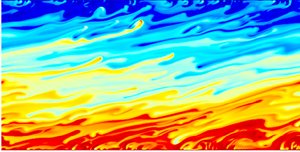
 $\varGamma =12$ in figure 2(b) demonstrates that hot plumes drift leftwards and cold plumes drift rightwards. This produces a strong horizontal shear in which, however, the vertical heat transport is low.
(a) Time evolution of  $Nu$ for the zonal flow state for
 $Ra=10^{8}$ and
 $Pr=10$ with
 $\varGamma =4$ (black line) and
 $\varGamma =12$ (red line). (b) Temperature snapshot for the zonal flow state for
 $Ra=10^{8}$,
 $Pr=10$,
 $\varGamma =12$. (c) Time evolution of
 $Nu$ for
 $Ra=10^{8}$,
 $Pr=10$,
 $\varGamma =64$. The three curves correspond to three separate simulations with random perturbations added to the initial temperature field. In all the cases, the flow undergoes a transition from zonal flow to convection roll states, for which
 $Nu$ is larger. (d) Temperature snapshots at different times denoted by the red dashed lines for the simulation indicated by the red curve in panel (c). At
 $t=2000$, there is zonal flow, whereas later it features an increasing number of turbulent convection rolls. (e) The final two-roll state for
 $Ra=10^{8}$,
 $Pr=10$,
 $\varGamma =128$, and the zoom in of the two plume-ejecting regions. For all these simulations the initial velocity had a linear shear flow profile
 $u(z)=2z-1, w=0$, in order to trigger a zonal flow state.

We now explore even larger aspect ratio domains. Figure 2(c) shows the time evolution of  $Nu$ for three separate simulations with random perturbations added to the initial temperature field for
 $Ra=10^{8}$ and
 $Pr=10$ in a
 $\varGamma =64$ cell. For all the three simulations, the zonal flow eventually evolves to a convection roll state. The time at which the transition occurs is very different for each simulation. The reason for that is that the flow is susceptible to small differences in the initial conditions, which are different for each simulation due to the random perturbations to the initial temperature field. Such sensitivity to the initial conditions is typical for chaotic systems and makes it impossible to predict when the transition will happen.
Figure 2(d) displays three temperature snapshots at different time instants indicated by the red dashed lines in figure 2(c). A complementary movie, showing how the zonal flow undergoes a transition towards a convection roll state, is given in the supplementary material available at https://doi.org/10.1017/jfm.2020.793. Initially, the hot plumes travel leftwards and the cold plumes rightwards. The transition starts when some local hot plumes are strong enough to deviate upwards and cross the whole fluid layer up to the collision with the upper cold plate. This prevents the further rightward motion of the neighbouring cold plumes, which instead start to move downwards. This process generates a local large-scale circulation, as is observed in the temperature field at  $t=4172$. The circulation grows over time until two stable convection rolls of equal size are formed, as seen in the temperature field at
 $t=5000$. Figure 2(e) shows that we also obtain a two-roll state for
 $\varGamma =128$, such that the horizontal extent of the convection roll is
 $64$ times the height of the convection cell, and this state is stable for more than 10 000 free-fall time units.
The cases in figure 2 use shear flow as the initial condition. If we use convection roll states as initial conditions, we can also obtain statistically stable convection roll states as indicated in figure 3 for different roll states for  $Ra=10^{8}$,
 $Pr=10$,
 $\varGamma =12$. So for this case, both zonal flow and different convection roll states can stably exist, depending on the initial conditions.
Temperature snapshots of different roll states for  $Ra=10^{8}$ and
 $Pr=10$ in a
 $\varGamma =12$ periodic cell. (a) Two-roll state; (b) four-roll state; (c) six-roll state; (d) eight-roll state. The different roll states are from initial conditions with different numbers of initial rolls.

We now explore the phase diagram for the different flow states in the parameter space spanned by  $Ra$,
 $Pr$ and
 $\varGamma$ (see figure 4 for the simulated cases). We find that in small-aspect ratio cells, only zonal flow is stable, while in large-aspect ratio cells, only convection roll states are stable. For intermediate aspect ratios, we find a regime in which both zonal flow and convection roll states are stable, depending on the initial conditions mentioned in § 2. We call this regime the bistable one. In order to map out an accurate phase diagram, we performed long simulations for the bistable cases with largest
 $\varGamma$ to conclude that the corresponding zonal flow can stably exist and does not evolve to a convection roll state. Overall, we ran the simulations for at least 50 000 free-fall time units for these cases, which corresponds to at least five viscous diffusive time units (
 $H^{2}/\nu$) or 0.5 thermal diffusive time units (
 $H^{2}/\kappa$). From figure 4(a) it can be seen that, when
 $Ra$ is increased, the bistable regime exists in an increasing
 $\varGamma$ range. This is also consistent with the finding that zonal flow develops more readily for higher
 $Ra$ for
 $\varGamma =2$ (Goluskin et al. Reference Goluskin, Johnston, Flierl and Spiegel2014). Figure 4(b) demonstrates that the
 $\varGamma$ range for the bistable state also depends on
 $Pr$. For
 $Ra = 10^{8}$ the largest range of bistable state exists at
 $Pr\sim 30$, namely between
 $\varGamma =3$ and
 $\varGamma =24$.
Phase diagram in the (a)  $Ra-\varGamma$ parameter space for
 $Pr=10$ and in the (b)
 $Pr-\varGamma$ parameter space for
 $Ra=10^{8}$. Black circles (
 $\bullet$) correspond to only zonal flow, red squares (
 ${_\square}$) denote coexistence of zonal flow and convection rolls, and blue diamonds (
 ${_\lozenge}$) indicate that only convection roll states are stable. The black hollow circles mark the cases shown in figure 2. Note that we also performed simulations for
 $Ra=10^{9}$,
 $Pr=10$ for convection roll states with
 $\varGamma =16$ and zonal flow state for
 $\varGamma =2$, to obtain
 $Nu\sim Ra^{\alpha }$ and
 $Re\sim Ra^{\beta }$ effective scaling relations for
 $Nu$ and
 $Re$.

We have already shown that zonal flow cannot be sustained, and only convection roll states are observed, when  $\varGamma$ is larger than a critical value, which depends on
 $Ra$ and
 $Pr$. A related question is how many convection rolls (in other words, what is the mean aspect ratio of individual convection rolls) can develop for a specific (
 $Ra$,
 $Pr$,
 $\varGamma$). In the next subsection, we will explore the possible convection roll states using different initial roll states generated by different Fourier basis, as explained in § 2.
3.2. Coexistence of multiple convection roll states at large $\varGamma$

In this subsection, we study the coexistence of multiple convection roll states in large-aspect ratio domains, all being statistically stable states once achieved. Figure 5 shows that for  $Ra=10^{8}$,
 $Pr=10$, and free-slip at the plates, in a
 $\varGamma =16$ system convection rolls with a mean dimensionless horizontal size of
 $1.6\leqslant \varGamma _r\leqslant 8$ are all statistically stable. The heat transport considerably increases with decreasing mean aspect ratio
 $\varGamma _r$ of an individual convection roll. For example, the heat transport for the
 $\varGamma _r=1.6$ state is almost twice as high as that for
 $\varGamma _r=8$. Although it had been observed before that convection rolls with smaller
 $\varGamma _r$ imply a higher heat transport – e.g. for 2-D RB convection with no-slip plates (van der Poel et al. Reference van der Poel, Stevens, Sugiyama and Lohse2012; Wang et al. Reference Wang, Wan, Yan and Sun2018a, Reference Wang, Verzicco, Lohse and Shishkina2020b), for RB convection in an annulus convection cell (Xie, Ding & Xia Reference Xie, Ding and Xia2018) and also for Taylor–Couette flow (Huisman et al. Reference Huisman, Van Der Veen, Sun and Lohse2014) – in those cases the observed increase in the transport is typically a couple of per cent, and by far not as large as observed for RB with free-slip plates and large aspect ratio cells as studied here. This difference is due to different plume dynamics and the associated spatial dependence of the local Nusselt number,
 $Nu(x)$, as we will discuss later.
Temperature snapshots of different roll states for  $Ra=10^{8}$ and
 $Pr=10$ in a
 $\varGamma =16$ periodic cell. The dimensionless mean horizontal size of the convection roll
 $\varGamma _r$ (i.e. the mean aspect ratio of one individual roll) and the Nusselt number
 $Nu$ for each state are indicated. The different roll states are from initial conditions with different numbers of initial rolls. All these states can stably exist for a long time (see table 3 in appendix A) without undergoing a transition to other states.

We also tested initial conditions with 12, 14, 16 rolls for  $Ra=10^{8},Pr=10,\varGamma =16$. These states with smaller rolls are not stable and will finally undergo a transition to the ten-roll state by merging of convection rolls. From figure 6(a) it is seen that the vertical Reynolds number
 $Re_z$ has a sudden decrease during merging of rolls, because the strong vertical motion is concentrated near the plume-ejecting regions between two neighbouring rolls. The decrease of
 $Nu$ during merging events can also be observed in figure 6(b), which is related to the decreased vertical motion. Figure 6(c) shows how the flow undergoes a transition from the initial sixteen-roll state to the final ten-roll state by successive merging of convection rolls. The transition happens when the balance of the roll state is broken by horizontal motion of local hot/cold plumes: in the second snapshot at
 $t=85$ the system is still in the initial sixteen-roll state. However, one can already see that a local hot plume moves leftwards while its neighbouring cold plume moves rightwards (marked by red arrows). In the third snapshot at
 $t=87$ two hot plumes merge to a single one and so do two cold ones, thus annihilating two rolls. The resulting fourteen-roll state is shown in the fourth snapshot taken at
 $t=141$. At later times the horizontal motion of the plumes and their further merging let the fourteen-roll state evolve to a twelve-roll state (
 $t=182$, III) and finally to a ten-roll state (
 $t=300$, IV). We also performed very long simulations as indicated in figure 6(d), from which we conclude that the ten-roll state can statistically stably exist for a very long time without undergoing any further transition to yet another state.
Time evolution of (a)  $Re$ and (b)
 $Nu$ for
 $Ra=10^{8}$,
 $Pr=10$,
 $\varGamma =16$ with an initial sixteen-roll state. Here,
 $Re_x=\sqrt {(Ra/Pr)}\sqrt {(\langle u^{2}\rangle _V)}$ is the horizontal Reynolds number and
 $Re_z=\sqrt {(Ra/Pr)}\sqrt {(\langle w^{2}\rangle _V)}$ the vertical one. (c) Temperature snapshots at different times. The roll merging can be seen, namely the flow undergoes a transition from the initial sixteen-roll state (I), to a fourteen-roll state (II), to a twelve-roll state (III) and then to the final ten-roll state (IV). The figure has the same colour scale as figure 5. (d) Time evolution of
 $Re$ for much longer time (on a log-scale) to show that the final ten-roll state is stable without undergoing a transition to another roll state.

Figure 7 displays phase diagrams for all the possible convection roll states in the  $Ra-\varGamma _r$ and
 $Pr-\varGamma _r$ parameter spaces. The stable roll states can last for several thousand free-fall time units without undergoing a transition to other states (see appendix A). Figure 7(a) shows a weak dependence of
 $\varGamma _r$ on
 $Ra$. One can observe the same stable roll states for the considered
 $Ra$ range. In contrast, a pronounced dependence of
 $\varGamma _r$ on
 $Pr$ is observed in figure 7(b), where convection roll states with the smallest
 $\varGamma _r$ are observed for intermediate
 $Pr\approx 10$. The minimum
 $\varGamma _r=16/11$ occurs for
 $\varGamma =32$, which means that the horizontal extent of a stable convection roll is always larger than the height of the system, also for smaller
 $\varGamma =8$, we found that the smallest roll size (
 $\varGamma _r=4/3$) is always larger than 1. This explains why convection rolls cannot be supported for small
 $\varGamma \approx 2$, where indeed only zonal flow was obtained. From figure 7(b) it can also be concluded that these results are independent of the aspect ratio of the system once it is large enough, as we obtained almost the same result for
 $\varGamma =16$ and
 $\varGamma =32$ domains.
Phase diagram for different roll states for (a)  $Pr=10$,
 $\varGamma =16$ and (b)
 $Ra=10^{8}, \varGamma =16$. Circles denote that the corresponding roll state with the mean aspect ratio
 $\varGamma _r$ of an individual roll is stable, while crosses denote that the roll state is not stable. The solid line in panel (b) connects the minimal mean aspect ratio
 $\varGamma _{r,\rm {min}}$ of an individual convection roll for different
 $Pr$ for
 $\varGamma =16$, while the dashed line connects
 $\varGamma _{r,min}$ for different
 $Pr$ for
 $\varGamma =32$.

3.3. Nusselt number and Reynolds number
We now discuss the effective scaling relations of  $Nu$ and
 $Re$ as function of
 $Ra$ and
 $Pr$. These relationships are usually expressed with effective scaling laws
 $Nu\sim Ra^{\gamma _{Nu}}Pr^{\alpha _{Nu}}$ and
 $Re\sim Ra^{\gamma _{Re}}Pr^{\alpha _{Re}}$ (Ahlers et al. Reference Ahlers, Grossmann and Lohse2009). The effective scaling laws have been widely discussed for no-slip cases for both 2-D and 3-D convection (Ahlers et al. Reference Ahlers, Grossmann and Lohse2009). For the 2-D horizontally periodic cases with no-slip plates,
 $Nu\sim Ra^{0.29}$ is found with
 $Pr=1, Ra\le 10^{10}$ (Johnston & Doering Reference Johnston and Doering2009; Zhu et al. Reference Zhu, Mathai, Stevens, Verzicco and Lohse2018a). For 2-D RB convection with no-slip plates and sidewalls with unit aspect ratio, several studies have shown that
 $Nu\sim Ra^{0.3}$ and
 $Re\sim Ra^{0.6}$ (Sugiyama et al. Reference Sugiyama, Calzavarini, Grossmann and Lohse2009; Zhang, Zhou & Sun Reference Zhang, Zhou and Sun2017; Wang et al. Reference Wang, Zhou, Wan and Sun2019c). However, how these effective scaling relations will change for free-slip plates has not been explored, especially not for convection roll states, which are only present in a large enough domain size.
Figures 8(a) and 8(b) show  $Nu$ and
 $Re$ as functions of
 $Ra$ for both zonal flow (
 $\varGamma =2$) and convection roll states (
 $\varGamma =16$) for
 $Pr=10$. Figure 8(a) reveals that the heat transfer in the convection roll state is much higher than that of the zonal flow state. Detailed information about the obtained scaling exponents is listed in table 2. For the convection roll states we find that the effective scaling exponent
 $\gamma _{Nu}$ in
 $Nu \sim Ra^{\gamma _{Nu}}$ is approximately
 $0.3$. It increases with increasing
 $\varGamma _r$, reaching approximately 1/3 for the largest
 $\varGamma _r=8$, which is the value predicated by the Grossmann–Lohse (GL) theory for the
 $\textrm {I}_\infty ^{<}$ and
 $\textrm {III}_\infty$ regimes (Grossmann & Lohse Reference Grossmann and Lohse2000, Reference Grossmann and Lohse2001; Shishkina et al. Reference Shishkina, Emran, Grossmann and Lohse2017) for the no-slip case. For zonal flow
 $\gamma _{Nu}$ is much smaller, namely only
 $0.17$. The effective scaling exponent
 $\gamma _{Re}$ in
 $Re \sim Ra^{\gamma _{Re}}$ is approximately
 $0.6$ for zonal flow and approximately
 $0.67$ for the convection roll state, which is also close to the GL predication of 2/3 for the
 $\textrm {I}_\infty ^{<}$ and
 $\textrm {III}_\infty$ regimes (Grossmann & Lohse Reference Grossmann and Lohse2001; Shishkina et al. Reference Shishkina, Emran, Grossmann and Lohse2017) for no-slip cases, while it is larger than
 $0.6$ that has been reported for 2-D RB convection with no-slip plates (Sugiyama et al. Reference Sugiyama, Calzavarini, Grossmann and Lohse2009; Zhang et al. Reference Zhang, Zhou and Sun2017; Wang et al. Reference Wang, Zhou, Wan and Sun2019c).
The (a)  $Nu$ and (b)
 $Re$ as functions of
 $Ra$ for different convection roll states (see legend in panel (d)) for
 $Pr=10$,
 $\varGamma =16$ and the zonal flow state (see orange stars on solid orange line) for
 $Pr=10$,
 $\varGamma =2$. The (c)
 $Nu$ and (d)
 $Re$ as functions of
 $Pr$ for different roll states for
 $Ra=10^{8}$,
 $\varGamma =16$ and for the zonal flow state, for which we put
 $\varGamma =2$. Again, see the legend in panel (d). The inset in panel (c) shows
 $Nu$ as a function of
 $\varGamma _r$ for
 $Ra=10^{8}$ and different
 $Pr$ obtained for
 $\varGamma =16$ (hollow symbols) and
 $\varGamma =32$ (solid symbols). The solid symbols often overshadow the hollow ones as the symbol sizes are the same.

The effective scaling exponents for fitted effective scaling relations  $Nu \sim Ra^{\gamma _{Nu}}$,
 $Re \sim Ra^{\gamma _{Re}}$ and
 $Re \sim Pr^{\alpha _{Re}}$ for different roll states for
 $Pr=10$ obtained in an aspect ratio
 $\varGamma =16$ domain. The zonal flow data is for
 $\varGamma =2$.

Next, we will discuss the Prandtl number dependence of the Nusselt number,  $Nu(Pr)$. For no-slip plates in 3-D cases, it is known that the
 $Nu$ is maximal around
 $Pr\sim 2\text {--}3$, and after that it declines with increasing
 $Pr$ (Ahlers & Xu Reference Ahlers and Xu2001; Xia, Lam & Zhou Reference Xia, Lam and Zhou2002; Stevens, Lohse & Verzicco Reference Stevens, Lohse and Verzicco2011). This remarkable maximum in
 $Nu(Pr)$ had in fact been predicted before by the GL theory (Grossmann & Lohse Reference Grossmann and Lohse2000, Reference Grossmann and Lohse2001). In contrast, for the 2-D cases, Huang & Zhou (Reference Huang and Zhou2013) showed that
 $Nu(Pr)$ has a minimum, rather than a maximum as in the 3-D case, namely at
 $Pr\sim 2\text {--}3$ for moderate
 $Ra$. This anomalous relation is caused by counter-gradient heat transport in 2-D cases.
What does the  $Nu(Pr)$ dependence look like for the 2-D RB case with free-slip plates? For the zonal flow state, Goluskin et al. (Reference Goluskin, Johnston, Flierl and Spiegel2014) already showed that
 $Nu$ is an increasing function of
 $Pr$ in the range
 $1\leqslant Pr\leqslant 10$. Figures 8(c) and 8(d) show the relations for
 $Nu(Pr)$ and
 $Re(Pr)$ for all states with free-slip plates (i.e. both for zonal flow and for various convection roll states). From figure 8(c) it can be seen that the
 $Nu(Pr)$ trend shown by Goluskin et al. (Reference Goluskin, Johnston, Flierl and Spiegel2014) is also valid for the wider range of
 $Pr$ analysed in this paper. The reason why
 $Nu$ is much smaller for small
 $Pr$ is that zonal flow features intermittent bursts whereas most of the time
 $Nu$ is around 1 (Goluskin et al. Reference Goluskin, Johnston, Flierl and Spiegel2014). For large
 $Pr$, the flow does not burst and convective heat transport with
 $Nu\gg 1$ is sustained at all times, thus the corresponding
 $Nu$ is larger than that of the small
 $Pr$ cases.
For the convection roll states, figure 8(c) shows that  $Nu$ increases monotonically with increasing
 $Pr$ for large mean convection roll size
 $\varGamma _r=16$ (see the inset). This can be interpreted as that the flow for the large
 $\varGamma _r=16$ cases can be viewed as ‘localized’ zonal flow, thus the
 $Nu(Pr)$ follows the similar trend as that of zonal flow. In contrast, for small
 $\varGamma _r$,
 $Nu$ decreases with increasing
 $Pr$. For
 $Re(Pr)$, figure 8(d) shows that the
 $Re$ follows
 $Re\sim Pr^{-1}$ for convection roll states (see table 2), the exponent,
 $-1$, is the same as that of the GL predication for the
 $\textrm {{I}}_\infty ^{<}$ and
 $\textrm {{III}}_\infty$ regimes for no-slip cases.
In order to understand different  $Nu(Pr)$ dependence for large and small
 $\varGamma _r$ as shown in figure 8(c), we first look at the flow organizations for convection roll states for different
 $Pr$. Figure 9(a) gives the time-averaged temperature fields for the
 $\varGamma _r=16$ roll state for different
 $Pr$. The flow near the bottom plate can be divided into the plume-ejecting region, the plume-impacting region, and between them there is a wind-shearing region which occupies a large fraction of the domain. In the ejecting region, thermal plumes are emitted, while in the impacting region, the boundary layer is impinged by the plumes from the opposite plate. The wind-shearing region is sheared by the large-scale circulation. The impacting regions on the top plate are the opposite of the ejecting regions of the bottom plate and vice versa. This kind of division is also adopted in periodic 2-D RB convection with no-slip plates (van der Poel et al. Reference van der Poel, Ostilla-Mónico, Verzicco, Grossmann and Lohse2015b). A remarkable observation is the stable stratification near the plume impacting region. Figure 9(c) shows a zoom-in of the regions where hot plumes are ejected for
 $Pr=1$ and 10. When hot fluid impinges the cold plate it does not have sufficient time to cool down before it moves horizontally. The consequence is that the temperature of the fluid between the top boundary layer and the bulk is higher than that of the bulk fluid, thus implying a stable stratification. This behaviour is even observed at the centreline of the hot plume (the vertical line at the horizontal location where the local bottom wall heat flux is minimal) as is shown in temperature profiles in figure 9(d), where for
 $Pr>1$ stable stratification near the cold plate is observed. The stable stratification has also been observed at the axis in cylindrical RB convection (Tilgner, Belmonte & Libchaber Reference Tilgner, Belmonte and Libchaber1993; Brown & Ahlers Reference Brown and Ahlers2007; Wan et al. Reference Wan, Wei, Verzicco, Lohse, Ahlers and Stevens2019) and in 2-D RB convection with no-slip plates and sidewalls for unit aspect ratio in the central region near the plates (Wan et al. Reference Wan, Wang, Wang, Xia, Zhou and Sun2020). The instantaneous temperature fields shown in figure 9(b) for
 $Pr=100$ reveals the ‘localized’ zonal flow structures. It can be seen that plumes are ejected everywhere while they can only move vertically and impinge the cold plate in the central region.
(a) Time-averaged temperature fields for the  $\varGamma _r=16$ roll state for different
 $Pr$ at
 $Ra=10^{8}$ obtained in a
 $\varGamma =32$ domain. (b) Instantaneous temperature field for
 $Pr=100$ for the
 $\varGamma _r=16$ state with
 $Ra=10^{8},\varGamma =32$. (c) Zoom-in for the time-averaged temperature fields in panel (a) for
 $Pr=1$ and 10. (d) Temperature profiles for the different
 $Pr$ at the centre point of plume-ejecting regions (
 $x/H\approx 16$) where the local
 $Nu$ is smallest. Panels (e) and (f) show the spatial dependence of
 $Nu(x)$ at the hot plate at
 $z=0$ (solid lines) and the cold plate at
 $z=1$ (dashed lines) for different
 $Pr$ for the (e)
 $\varGamma _r=16$ and the (f)
 $\varGamma _r=4$ roll states. Note that all curves are shifted such that the minimum local
 $Nu$ at the hot plate is located at
 $x/H=16$.

Next, we focus on the local properties of the wall heat flux. The local wall heat flux is expressed through the local wall Nusselt number  $Nu(x)|_{z=0,1}=\partial \left \langle \theta \right \rangle _t/\partial z|_{z=0,1}$. Figures 9(e) and 9(f) show the spatial
 $Nu(x)$ dependence at the plates for
 $Ra=10^{8}$ and
 $\varGamma =32$ for
 $\varGamma _r=16$ and
 $\varGamma _r=4$, respectively. For small
 $Pr=1$, one sees from figure 9(a) the accumulation of hot fluid in the ejecting region near the bottom plate, which causes a small temperature gradient (see figure 9d), and correspondingly small local
 $Nu$ (see figure 9e). So the centre of the ejecting region can be denoted as the point where local wall heat flux is minimal. In contrast, for the impacting region (
 $x/H\approx 0$ at the bottom plate) where cold fluid directly impinges the hot plate, there is a sharp temperature gradient and thus large local
 $Nu$ (see figure 9e). Similar
 $Nu$ behaviour is also observed in the ejecting/impacting regions near the top plate (dashed lines in figure 9e). The physical interpretation is as follows: the heat is ejected into the system through the bottom plate mainly at the plume-impacting regions where the local temperature gradient is large, and then it is advected by large-scale circulation to the plume-ejecting regions, where the conductive heat flux is low on the wall, while the convective heat flux is high above the wall. The heat is mainly removed from the system when the hot plume impinges the cold plate.
For  $\varGamma _r=16$, there is only one impacting region near the bottom plate, and the heat input is still dominated by the wind-shearing region, which occupies a large fraction of the domain. As the wind-shearing region is like ‘localized’ zonal flow where
 $Nu$ increases with increasing
 $Pr$, the global
 $Nu$ thus also increases with increasing
 $Pr$. In contrast, for smaller
 $\varGamma _r$, there are more impacting regions on the bottom plate, and these impacting regions contribute significantly to the global heat input. As the heat flux at the impacting region increases with decreasing
 $Pr$, we thus see that the global
 $Nu$ also increases with decreasing
 $Pr$.
4. 3-D simulations
We have already shown that the zonal flow observed in 2-D RB convection with free-slip plates and horizontally periodic boundary conditions for  $\varGamma =2$ (Goluskin et al. Reference Goluskin, Johnston, Flierl and Spiegel2014; van der Poel et al. Reference van der Poel, Ostilla-Mónico, Verzicco and Lohse2014) eventually disappears with increasing
 $\varGamma$. What about in 3-D, under the same conditions? For the 3-D RB convection with free-slip plates, previous studies have not reported zonal flow (Petschel et al. Reference Petschel, Stellmach, Wilczek, Lülff and Hansen2013; Kunnen et al. Reference Kunnen, Ostilla-Mónico, van der Poel, Verzicco and Lohse2016). However, if we introduce spanwise rotation as illustrated in figure 1(b) where the rotating axis is parallel to the
 $y$ axis, the flow will become 2-D-like at sufficiently fast rotation, due to the Taylor–Proudman theorem. In this way we may observe zonal flow at certain parameters, as indeed was already reported in von Hardenberg et al. (Reference von Hardenberg, Goluskin, Provenzale and Spiegel2015). Therefore, here we will study spanwise rotating RB convection, focusing on the transition from zonal flow to convection roll states with increasing aspect ratio
 $\varGamma$ of the container.
We first show that both the global transport properties like the Nusselt number  $Nu$ and the Reynolds number
 $Re$, as well as the flow organization, increasingly behave like 2-D cases with increasing rotation rate. We fix the Rayleigh number to
 $Ra=10^{7}$ and the Prandtl number to
 $Pr=0.71$. To be on the safe side, we choose a large domain with
 $\varGamma =16$, as previous studies showed that large aspect ratios are needed in order to capture the superstructures which have a horizontal size of 6–7 times the height of the domain for 3-D RB convection with no-slip plates (Pandey et al. Reference Pandey, Scheel and Schumacher2018; Stevens et al. Reference Stevens, Blass, Zhu, Verzicco and Lohse2018; Green et al. Reference Green, Vlaykov, Mellado and Wilczek2020; Krug et al. Reference Krug, Lohse and Stevens2020). The initial conditions have zero velocity and a linear temperature profile for these simulations. For RB convection rotating about a vertical axis for small
 $Pr=0.71$ with no-slip plates,
 $Nu$ initially does not change much with an increasing of the rotation rate (denoted by the inverse Rossby number
 $1/Ro$), until after
 $1/Ro\geqslant 1$,
 $Nu$ drops monotonically with increasing
 $1/Ro$ (Zhong et al. Reference Zhong, Stevens, Clercx, Verzicco, Lohse and Ahlers2009). Figure 10(a) shows that for spanwise rotating RB convection,
 $Nu$ also initially does not change much for
 $1/Ro\leqslant 1$. After that,
 $Nu$ drops monotonically until reaching its minimum at
 $1/Ro \approx 10$, and then it increases monotonically towards the 2-D value for a two-roll state. Similar non-monotonic behaviour of
 $Nu$ with the control parameter was also found in sheared RB convection, where
 $Nu$ also non-monotonically depends on the wall shear Reynolds number (Blass et al. Reference Blass, Zhu, Verzicco, Lohse and Stevens2020). For spanwise rotating RB convection,
 $Re$ monotonically increases from the 3-D value towards the 2-D value with increasing rotation rate, as shown in figure 10(b). Note that this behaviour is very different from RB convection rotating around the vertical axis, where
 $Re$ decreases monotonically with increasing
 $1/Ro$ (Chong et al. Reference Chong, Yang, Huang, Zhong, Stevens, Verzicco, Lohse and Xia2017).
The 3-D RB convection with spanwise rotation: (a)  $Nu$ and (b)
 $Re$ as functions of
 $1/Ro$ for
 $Ra=10^{7},Pr=0.71,\varGamma =16$ (black circles). For orientation with respect to the Nusselt number, the data for non-rotation (
 $1/Ro=0$, red diamond) and the 2-D cases with the same control parameters (
 $Ra=10^{7}$,
 $Pr=0.71$,
 $\varGamma =16$) for different roll aspect ratios
 $\varGamma _r$ (blue squares) are also shown; for these data points the value at the
 $1/Ro$ axis has no meaning. The Reynolds number,
 $Re$, for the
 $\varGamma _r=8/3$ (7702.85) and
 $\varGamma _r=2$ (7726.20) states are close to each other and cannot be differentiated in the figure.

We now connect the global transport properties with the flow organization. Figure 11 shows instantaneous temperature fields at the midheight (top row) and boundary layer height close to the bottom plate (bottom row) for different  $1/Ro$ with
 $Ra=10^{7}, Pr=0.71,\varGamma =16$. We can clearly see the connection between large-scale thermal structure at midheight and boundary layer height for different
 $1/Ro$, which has also been shown in 3-D RB convection with no-slip plates (Stevens et al. Reference Stevens, Blass, Zhu, Verzicco and Lohse2018; Green et al. Reference Green, Vlaykov, Mellado and Wilczek2020). With increasing rotation rate, one sees the increasing two-dimensionlization of the flow. For the non-rotation case (
 $1/Ro=0$), figure 11(a) shows qualitatively similar superstructures as the no-slip case (Pandey et al. Reference Pandey, Scheel and Schumacher2018; Stevens et al. Reference Stevens, Blass, Zhu, Verzicco and Lohse2018). When
 $1/Ro$ increases to 1, a meandering large-scale convection roll state develops, as can be seen from figure 11(b). Interestingly, similar meandering structures have also been observed in many shear-driven flows when the horizontal isotropy is broken, such as plane Couette flow (Lee & Moser Reference Lee and Moser2018), wavy Taylor rolls in Taylor–Couette flow (Andereck, Liu & Swinney Reference Andereck, Liu and Swinney1986) and also in sheared RB convection (Blass et al. Reference Blass, Zhu, Verzicco, Lohse and Stevens2020). Figure 10(a) shows that this meandering structure at
 $1/Ro=1$ still has similar
 $Nu$, as in the non-rotation case. For medium rotation rates
 $1/Ro=3.75$ and 10, a two-roll state evolves; interestingly, the cyclonic circulation has a larger size than the anticyclonic one. The smaller
 $Nu$ for these two-roll states is related to the decreased plume emission area. With further increasing rotation rate, the flow increasingly behaves like 2-D cases. For the largest
 $1/Ro=50$ as shown in figure 11(e), a two-roll state with equal size of each roll has developed, with small spanwise variation in temperature.
The 3-D RB convection with spanwise rotation (the rotating axis is parallel to  $y$ axis): top view snapshots of temperature fields at midheight (
 $z=H/2$, top row) and thermal boundary layer height (
 $z= z_{bl} = H/ (2 Nu$), bottom row) for
 $Ra=10^{7},Pr=0.71,\varGamma =16$ with different rotation rates. (a)
 $1/Ro=0$; (b)
 $1/Ro=1$; (c)
 $1/Ro=3.75$; (d)
 $1/Ro=10$; (e)
 $1/Ro=50$.

After we have shown the increasing two-dimensionalization of the flow with increasing rotation rate for spanwise rotating RB convection, next we will study the transition from zonal flow to the convection roll states with increasing aspect ratio  $\varGamma$, similarly as we have already done for the 2-D case. von Hardenberg et al. (Reference von Hardenberg, Goluskin, Provenzale and Spiegel2015) studied spanwise rotating RB convection for
 $Ra=10^{7},Pr=0.71$ with fixed
 $\varGamma =2{\rm \pi}$. They observed strong zonal flow that is perpendicular to both rotation vector and gravity vector. Both the cyclonic zonal flow and the anticyclonic one have been obtained using different initial conditions. These two kinds of zonal flow are symmetric for 2-D cases, while they are not in 3-D cases with spanwise rotation, as the Coriolis force depends on the direction of velocity and thus it breaks the symmetry between the two kinds of zonal flow, which have an opposite flow direction. The main difference between the two kinds of zonal flow is that intermittent bursts exist for anticyclonic zonal flow, similar to what is observed in 2-D cases with small
 $Pr\le 2$, while these bursts are absent for the cyclonic zonal flow (von Hardenberg et al. Reference von Hardenberg, Goluskin, Provenzale and Spiegel2015). We note that, as in von Hardenberg et al. (Reference von Hardenberg, Goluskin, Provenzale and Spiegel2015), the dimensionless angular velocity
 $\varOmega ^{\prime }=\varOmega \tau _{th}$ is used to quantify the rotation velocity, where
 $\tau _{th}=H^{2}/\kappa$ is thermal diffusive time. The dimensionless angular velocity is related to the Rossby number by
 $Ro=\sqrt {RaPr}/(2\varOmega ^{\prime })$ (Novi et al. Reference Novi, von, Jost, David, Provenzale and Spiegel2019).
We performed simulations for  $Ra=10^{7}$,
 $Pr=0.71$,
 $\varGamma =8$ and 16 with
 $1/Ro=3.75$, which corresponds to
 $2\varOmega ^{\prime }=10\,000$ in von Hardenberg et al. (Reference von Hardenberg, Goluskin, Provenzale and Spiegel2015). Three different initial conditions were used to trigger different possible states, namely:
(i)
${{IC}}_0$ with zero initial velocity;(ii)
${{IC}}_c$ with cyclonic shear flow $u(z)=2z-1$, $v=0$, $w=0$, to trigger possible cyclonic zonal flow; and(iii)
${{IC}}_a$ with anticyclonic shear flow $u(z)=1-2z$, $v=0$, $w=0$, to trigger possible anticyclonic zonal flow.


We first report the results for  $\varGamma = 8$: figure 12(a) illustrates that for the initial conditions
 ${{IC}}_0$, the flow quickly develops into a two-roll state as indicated in figure 12(c). We note that the cyclonic circulation is again larger than the anticyclonic one. For
 ${IC}_c$ as initial conditions, the cyclonic zonal flow shown in figure 12(d) can statistically stably exist for more than 3000 free-fall time units. Finally, the initial conditions
 ${{IC}}_a$ can trigger an anticyclonic zonal flow with burst phenomenon, which is consistent with the findings of von Hardenberg et al. (Reference von Hardenberg, Goluskin, Provenzale and Spiegel2015). However, here this feature only lasts for approximately 380 free-fall time units and then the system undergoes a transition to a two-roll state. We thus conclude that for
 $\varGamma =8$ the system can again display a bistability behaviour, in which both zonal flow and convection roll states are statistically stable.
The 3-D RB convection with spanwise rotation (the rotating axis is parallel to  $y$ axis): time evolution of
 $Nu$ for
 $Ra=10^{7}, Pr=0.71, 1/Ro=3.75$ with three different initial conditions for (a)
 $\varGamma =8$ and (b)
 $\varGamma =16$. Here,
 ${{IC}}_{0}$ means the initial condition with zero velocity and
 ${{IC}}_c/ {{IC}}_{a}$ denote cyclonic/anticyclonic shear flow as the initial condition. (c–h) Side-view temperature snapshots at midspanwise length (
 $y/H=\varGamma /2$) at different times denoted by the dashed lines in panel (a,b).

We now come to the case of  $\varGamma =16$. From figure 12(b) we conclude that for three different initial conditions, the flow eventually evolves to the very same final state, namely the convection roll state. The cyclonic zonal flow initially seen for short time for the initial conditions
 ${IC}_c$ quickly undergoes a transition to the convection roll state. The snapshots in figure 12(b–d) reveal similar transition processes, as we had already observed in 2-D cases. Again, the final two-roll state has a larger cyclonic circulation. For the final convection state the horizontal scale of the flow reaches the domain size of 16, which is much larger than the typical horizontal scale of superstructures observed in 3-D RB convection with no-slip plates (Pandey et al. Reference Pandey, Scheel and Schumacher2018; Stevens et al. Reference Stevens, Blass, Zhu, Verzicco and Lohse2018). Such large-scale structures cannot be captured in small domains, which is the reason why for small domains only zonal flow states can be realized (von Hardenberg et al. Reference von Hardenberg, Goluskin, Provenzale and Spiegel2015).
To summarize our results from our 3-D simulations with free-slip plates and spanwise rotation (with fixed  $Ra=10^{7}$,
 $Pr=0.71$, and relative strong rotation
 $1/Ro=3.75$), we have revealed a similar physical picture as we had done before for 2-D RB convection with free-slip plates:
(i) for small aspect ratio
$\varGamma =2{\rm \pi}$, the flow is zonal (von Hardenberg et al. Reference von Hardenberg, Goluskin, Provenzale and Spiegel2015);(ii) with increasing
$\varGamma$ up to at least $\varGamma = 8$, the convection roll state and the zonal flow state coexist in phase space and which one is taken depends on the initial conditions; and(iii) for larger
$\varGamma =16$, we always obtain the convection roll state, independently on of what kind of initial conditions were employed.


5. Concluding remarks
In summary, we have studied 2-D RB convection and spanwise rotating RB convection with free-slip plates in horizontally periodic domains using direct numerical simulations. Based on the present data, we find that the zonal flow, which was previously observed in a  $\varGamma =2$ cell (Goluskin et al. Reference Goluskin, Johnston, Flierl and Spiegel2014; van der Poel et al. Reference van der Poel, Ostilla-Mónico, Verzicco and Lohse2014), cannot be sustained and will undergo transitions to convection roll states when the aspect ratio
 $\varGamma$ is larger than a critical value, which depends on the Rayleigh number
 $Ra$ and Prandtl number
 $Pr$.
We reveal three regimes:
(i) for small
$\varGamma$ (typically $\varGamma \leqslant 1\text {--}3$, depending on $Ra$ and $Pr$), only zonal flow can be observed;(ii) with increasing
$\varGamma$, we first find a bistable regime in which, depending on the initial conditions, both zonal flow and convection roll states can be stable; and(iii) for even larger-aspect ratio systems, only convection roll states can be sustained.


How many convection rolls develop in the convection roll states (in other words, what is the mean aspect ratio  $\varGamma _r$ of an individual roll) depends on the initial conditions. For instance, for
 $Ra=10^{8}$ and
 $Pr=10$ the horizontal extent of the stable convection rolls varies between
 $16/11$ and
 $64$ times the height of the convection cell. A convection roll with an as large aspect ratio of
 $\varGamma _r = 64$, or more generally already with
 $\varGamma _r \gg 10$, can be seen as ‘localized’ zonal flow.
The heat transfer in the system increases significantly when the horizontal extent of the convection roll is reduced. It is found that the Prandtl number dependence of the Nusselt number  $Nu(Pr)$ has very different trends for large and small
 $\varGamma _r$: for large
 $\varGamma _r$ (like
 $\varGamma _r=16$ for a
 $\varGamma =32$ cell), the flow behaves like a ‘localized’ zonal flow state, and
 $Nu$ increases with increasing
 $Pr$, similarly as we found for the zonal flow state. In contrast, for small
 $\varGamma _r$, the heat flux into the system is dominated by the plume-impacting regions on the bottom plate, in which the local heat flux is very high and increases with decreasing
 $Pr$, implying that the global heat flux
 $Nu$ also increases with decreasing
 $Pr$.
For spanwise rotating 3-D RB convection, we find that with increasing rotation rate  $1/Ro$, both the transport properties (such as the Nusselt number
 $Nu$ and the Reynolds number
 $Re$) and the flow organization increasingly behave like in the corresponding 2-D cases. In particular, just as in the 2-D cases, the zonal flow observed in a small periodic cell with
 $\varGamma =2{\rm \pi}$ (von Hardenberg et al. Reference von Hardenberg, Goluskin, Provenzale and Spiegel2015), disappears in larger cells with
 $\varGamma =16$. For intermediate
 $\varGamma =8$, bistability is observed, again similarly as observed in 2-D RB convection.
Finally, an interesting but still open question is the final fate of the aspect ratio dependence of the zonal flow for higher  $Ra$: Is there a finite
 $Ra$ above which zonal flow exists for all
 $\varGamma$? On the one hand, for fixed
 $Ra$ within our explored range
 $Ra\leqslant 3\times 10^{8}$, zonal flow always seems to disappear when
 $\varGamma$ is sufficiently large; on the other hand, for fixed
 $\varGamma$, zonal flow always seems to stably exist when
 $Ra$ is large enough. We have to conclude that in spite of our efforts it still is an open question whether zonal flow can exist for all
 $\varGamma$ for a large enough but finite Rayleigh number. Due to the chaotic nature of the flow, mapping out the parameter regime where zonal flow can be found is not easy, especially not for high
 $Ra$ and large
 $\varGamma$.
From a broader perspective, our study underlines the importance of having large enough aspect ratios in numerical simulations of wall-bounded turbulent flows, even when one employs periodic boundary conditions. We had seen this before in 3-D RB convection with no-slip velocity boundary conditions at the plates (Pandey et al. Reference Pandey, Scheel and Schumacher2018; Stevens et al. Reference Stevens, Blass, Zhu, Verzicco and Lohse2018; Green et al. Reference Green, Vlaykov, Mellado and Wilczek2020; Krug et al. Reference Krug, Lohse and Stevens2020), but apparently this conclusion is much more general.
Acknowledgements
We thank O. Shishkina and D. Goluskin for fruitful discussions. Q.W. acknowledges financial support from the China Scholarship Council (CSC) and the Natural Science Foundation of China under grant no. 11621202. K.L.C. acknowledges the Croucher Foundation for the Croucher Fellowships for Postdoctoral Research. R.J.A.M.S. acknowledges the financial support from ERC (the European Research Council) Starting Grant no. 804283 UltimateRB. We acknowledge PRACE for awarding us access to MareNostrum 4 based in Spain at the Barcelona Computing Center (BSC) under Prace project 2018194742 and to Marconi based in Italy at CINECA under PRACE project 2019204979. This work was partly carried out on the national e-infrastructure of SURFsara, a subsidiary of SURF cooperation, the collaborative ICT organization for Dutch education and research.
Declaration of interests
The authors report no conflict of interest.
Supplementary material
Supplementary material is available at https://doi.org/10.1017/jfm.2020.793.
Appendix A. Tables with simulation details
Simulation details for all cases shown in figure 7(a). The columns from left to right indicate  $Ra$,
 $Pr$,
 $\varGamma$, grid resolutions
 $N_x\times N_z$, the number of initial rolls
 $n^{(i)}$, the number of final convection rolls
 $n$, the mean aspect ratio of the convection rolls
 $\varGamma _r=\varGamma /n$, the Nusselt number
 $Nu$, the Reynolds number
 $Re$ based on root mean square of the global velocity, the horizontal Reynolds number
 $Re_x$ based on root mean square of the horizontal velocity, the vertical Reynolds number
 $Re_z$, the total simulation time
 $t_{tot}$, and the time
 $t_{avg}$ used to average
 $Nu$ and
 $Re$.

Simulation details for the main cases in figure 7(b) for  $\varGamma =16$ and 32. The table head is the same as table 3. Here, ‘s’ denotes that the final flow state is steady, which means that both Nu and Re are independent of time once the final state is achieved.

Appendix B. Reynolds number ratio
Figure 13(a) shows the Reynolds number ratio  $Re_z/Re_x$ as a function of
 $\varGamma$ for the zonal flow state. The ratio
 $Re_z/Re_x$ increases with increasing
 $Pr$ for
 $Pr\geqslant 10$, which has a similar trend as
 $Nu$ discussed before. Figure 13(b) shows Reynolds number ratio
 $Re_z/Re_x$ as a function of
 $\varGamma _r$ for convection roll states for
 $Ra=10^{8}$ with different
 $Pr$. It is remarkable that
 $Re_z/Re_x$ seems to have a universal dependence on
 $\varGamma _r$ for different
 $Pr$, despite that
 $Nu$ has a different trend on
 $Pr$ for large and small
 $\varGamma _r$. The data can be well represented by the effective scaling relation
 $Re_z/Re_x = 0.86\varGamma _r^{-0.68}$.
(a) Reynolds number ratio  $Re_z/Re_x$ as a function of
 $\varGamma$ for the zonal flow state and (b) Reynolds number ratio
 $Re_z/Re_x$ as a function of
 $\varGamma _r$ for the convection roll state for
 $Ra=10^{8}$ with different
 $Pr$. Solid symbols in panel (b) for
 $\varGamma =16$ and hollow symbols for
 $\varGamma =32$. The solid symbols can hardly be seen as they are mostly hidden by the hollow symbols. The data in panel (b) can be well described by the effective scaling relation
 $Re_z/Re_x=0.86\varGamma _r^{-0.68}$.

Simulations details for 3-D RB convection with spanwise rotation. The corresponding 2-D simulations are also included for comparison. The table head is similar to that of tables 3 and 4, apart from the inverse Rossby number  $1/Ro$ for the 3-D cases. Here,
 ${IC_0}$ means initial conditions with zero velocity and conductive temperature profile with random perturbations and
 ${IC_c}$ means initial conditions with cyclonic shear flow
 $u(z)=2z-1$,
 $v=0$,
 $w=0$ and conductive temperature profile with random perturbations.


 Open access

