3.1 Data assimilation of the mean velocity fields

The experimental means are data assimilated using the framework devised by Foures et al. (Reference Foures, Dovetta, Sipp and Schmid2014) so that they can later be used as an input to resolvent analysis. Only the equations are reviewed here as its application to experimental data is discussed by Symon et al. (Reference Symon, Dovetta, McKeon, Sipp and Schmid2017). The flow is governed by the incompressible Navier–Stokes equations, which are non-dimensionalised by the free-stream velocity $U_{\infty }$ and the airfoil chord $c$ ,

(3.1a ) $$\begin{eqnarray}\displaystyle & \displaystyle \unicode[STIX]{x2202}_{t}\boldsymbol{u}+\boldsymbol{u}\boldsymbol{\cdot }\unicode[STIX]{x1D735}\boldsymbol{u}=-\unicode[STIX]{x1D735}p+Re^{-1}\unicode[STIX]{x1D6FB}^{2}\boldsymbol{u}, & \displaystyle\end{eqnarray}$$

(3.1b ) $$\begin{eqnarray}\displaystyle & \displaystyle \unicode[STIX]{x1D735}\boldsymbol{\cdot }\boldsymbol{u}=0, & \displaystyle\end{eqnarray}$$

$\boldsymbol{u}$

$p$

$u$

$v$

$w$

$x$

$y$

$z$

$\boldsymbol{u}=\overline{\boldsymbol{u}}+\boldsymbol{u}^{\prime }$

(3.2a ) $$\begin{eqnarray}\displaystyle & \displaystyle \overline{\boldsymbol{u}}\boldsymbol{\cdot }\unicode[STIX]{x1D735}\overline{\boldsymbol{u}}+\unicode[STIX]{x1D735}\overline{p}-Re^{-1}\unicode[STIX]{x1D6FB}^{2}\overline{\boldsymbol{u}}=\boldsymbol{f}=-\unicode[STIX]{x1D735}\boldsymbol{\cdot }\unicode[STIX]{x1D64D}, & \displaystyle\end{eqnarray}$$

(3.2b ) $$\begin{eqnarray}\displaystyle & \displaystyle \unicode[STIX]{x1D735}\boldsymbol{\cdot }\overline{\boldsymbol{u}}=0. & \displaystyle\end{eqnarray}$$

$\boldsymbol{f}$

$\unicode[STIX]{x1D64D}$

The data-assimilation algorithm treats $\boldsymbol{f}$ as an unknown and leverages partial knowledge of $\overline{\boldsymbol{u}}$ to reconstruct not only $\boldsymbol{f}$ but also $\overline{\boldsymbol{u}}$ on a larger domain which obeys prescribed boundary conditions. A constrained optimisation problem is formulated as follows:

(3.3) $$\begin{eqnarray}{\mathcal{L}}(\overline{\boldsymbol{u}}^{\dagger },\overline{p}^{\dagger },\overline{\boldsymbol{u}},\overline{p},\boldsymbol{f})={\mathcal{E}}(\overline{\boldsymbol{u}})-\langle \overline{\boldsymbol{u}}^{\dagger },\overline{\boldsymbol{u}}\boldsymbol{\cdot }\unicode[STIX]{x1D735}\overline{\boldsymbol{u}}+\unicode[STIX]{x1D735}\overline{p}-Re^{-1}\unicode[STIX]{x1D6FB}^{2}\overline{\boldsymbol{u}}-\boldsymbol{f}\rangle -\langle \overline{p}^{\dagger },\unicode[STIX]{x1D735}\boldsymbol{\cdot }\overline{\boldsymbol{u}}\rangle ,\end{eqnarray}$$

to minimise the difference between a measurement of $\overline{\boldsymbol{u}}$ , which satisfies (3.2), and the experimental mean velocity field $\overline{\boldsymbol{u}}_{exp}$ measurement. In (3.3), $(\cdot )^{\dagger }$ signifies an adjoint quantity and $\langle \boldsymbol{a}\boldsymbol{\cdot }\boldsymbol{b}\rangle =\int _{\unicode[STIX]{x1D6FA}}\boldsymbol{a}\boldsymbol{\cdot }\boldsymbol{b}\,\text{d}\unicode[STIX]{x1D6FA}$ . The scalar ${\mathcal{E}}$ quantifies the discrepancy and is given by

(3.4) $$\begin{eqnarray}{\mathcal{E}}(\overline{\boldsymbol{u}})={\textstyle \frac{1}{2}}\Vert \overline{\boldsymbol{m}}-{\mathcal{M}}(\overline{\boldsymbol{u}})\Vert _{M}^{2}.\end{eqnarray}$$

The operator ${\mathcal{M}}$ projects the numerical data to the subspace spanned by the known PIV measurements $\overline{\boldsymbol{m}}$ .

The variations of ${\mathcal{L}}$ with respect to each dependent variable are set to zero to obtain the equations which are solved iteratively until ${\mathcal{E}}$ is minimised. These include

(3.5a ) $$\begin{eqnarray}\displaystyle & \displaystyle -\overline{\boldsymbol{u}}\boldsymbol{\cdot }\unicode[STIX]{x1D735}\overline{\boldsymbol{u}}^{\dagger }+(\unicode[STIX]{x1D735}\overline{\boldsymbol{u}})^{T}\boldsymbol{\cdot }\overline{\boldsymbol{u}}^{\dagger }-\unicode[STIX]{x1D735}\overline{p}^{\dagger }-Re^{-1}\unicode[STIX]{x1D6FB}^{2}\overline{\boldsymbol{u}}^{\dagger }=\unicode[STIX]{x1D6FF}{\mathcal{E}}/\unicode[STIX]{x1D6FF}\overline{\boldsymbol{u}}, & \displaystyle\end{eqnarray}$$

(3.5b ) $$\begin{eqnarray}\displaystyle & \displaystyle \unicode[STIX]{x1D735}\boldsymbol{\cdot }\overline{\boldsymbol{u}}^{\dagger }=0, & \displaystyle\end{eqnarray}$$

(3.5c ) $$\begin{eqnarray}\displaystyle & \displaystyle \unicode[STIX]{x1D735}_{\boldsymbol{f}}{\mathcal{E}}=\overline{\boldsymbol{u}}^{\dagger }, & \displaystyle\end{eqnarray}$$

$\boldsymbol{f}$

$\unicode[STIX]{x1D735}\times \boldsymbol{f}$

The direct and adjoint RANS equations are solved in FreeFem++ (Hecht Reference Hecht2012) on the computational domain $\unicode[STIX]{x1D6FA}\in -5\leqslant x\leqslant 15\cup -5\leqslant y\leqslant 5$ with the leading edge of the airfoil being centred at the origin. The equations are spatially discretised using quadratic basis functions for the velocity and linear basis functions for the pressure resulting in approximately 360 000 and 1 000 000 degrees of freedom for the A0 and A10 cases, respectively.

3.2 Spectral proper orthogonal decomposition

The velocity fluctuations obtained from the processed PIV datasets are analysed using two modal decomposition techniques. The first, introduced by Lumley (Reference Lumley, Yaglom and Tatarski1967, Reference Lumley1970), is spectral proper orthogonal decomposition. From the raw, experimental data, SPOD calculates energy-ranked modes which are orthogonal to one another and oscillate at a single frequency. The SPOD modes are computed using the procedure described in Towne et al. (Reference Towne, Schmidt and Colonius2018) and the code developed by Schmidt & Towne (Reference Schmidt and Towne2019). A brief summary of the steps is presented below.

The PIV data are rearranged into the matrix

(3.6) $$\begin{eqnarray}\boldsymbol{Q}=\left[\begin{array}{@{}cccc@{}}\boldsymbol{q}_{1} & \boldsymbol{q}_{2} & \cdots \, & \boldsymbol{q}_{n}\end{array}\right]\in \mathbb{R}^{m\times n},\end{eqnarray}$$

where $m$ represents the number of states, i.e. the streamwise and transverse velocity of all PIV vectors, and $n$ is the total number of snapshots. Thus, the overall size of $\boldsymbol{Q}$ is 49 104 total states by 6800 snapshots. Following Welch’s method (Welch Reference Welch1967), $\boldsymbol{Q}$  is split into $p$ smaller, overlapping segments, or blocks, containing $n_{b}$ snapshots where $n_{b}<n$

(3.7) $$\begin{eqnarray}\boldsymbol{Q}^{(p)}=\left[\begin{array}{@{}cccc@{}}\boldsymbol{q}_{1}^{(p)} & \boldsymbol{q}_{2}^{(p)} & \cdots \, & \boldsymbol{q}_{n_{b}}^{(p)}\end{array}\right]\in \mathbb{R}^{m\times n_{b}}.\end{eqnarray}$$

Each row of $\boldsymbol{Q}^{(p)}$ is then Fourier transformed in time using the discrete Fourier transform (DFT), yielding an ensemble of Fourier realisations

(3.8) $$\begin{eqnarray}\hat{\boldsymbol{Q}}^{(p)}=\left[\begin{array}{@{}cccc@{}}\hat{\boldsymbol{q}}_{\unicode[STIX]{x1D714}_{1}}^{(p)} & \hat{\boldsymbol{q}}_{\unicode[STIX]{x1D714}_{2}}^{(p)} & \cdots \, & \hat{\boldsymbol{q}}_{\unicode[STIX]{x1D714}_{n_{b}}}^{(p)}\end{array}\right]\in \mathbb{C}^{m\times n_{b}}.\end{eqnarray}$$

The columns of $\hat{\boldsymbol{Q}}^{(p)}$ represent a Fourier mode instead of a snapshot in time as they did in $\boldsymbol{Q}^{(p)}$ . The Fourier modes for a specific frequency $\unicode[STIX]{x1D714}$ can be arranged into a new data matrix

(3.9) $$\begin{eqnarray}\hat{\boldsymbol{Q}}(\unicode[STIX]{x1D714})=\left[\begin{array}{@{}cccc@{}}\hat{\boldsymbol{q}}_{\unicode[STIX]{x1D714}}^{(1)} & \hat{\boldsymbol{q}}_{\unicode[STIX]{x1D714}}^{(2)} & \cdots \, & \hat{\boldsymbol{q}}_{\unicode[STIX]{x1D714}}^{(b)}\end{array}\right]\in \mathbb{C}^{m\times b},\end{eqnarray}$$

where $b$ is the number of blocks.

The cross-spectral density matrix for a specific temporal frequency $\hat{\boldsymbol{S}}(\unicode[STIX]{x1D714})$ is

(3.10) $$\begin{eqnarray}\hat{\boldsymbol{S}}(\unicode[STIX]{x1D714})=\hat{\boldsymbol{Q}}(\unicode[STIX]{x1D714})\hat{\boldsymbol{Q}}^{\ast }(\unicode[STIX]{x1D714})\in \mathbb{R}^{m\times m}.\end{eqnarray}$$

The SPOD eigenvectors $\hat{\boldsymbol{V}}(\unicode[STIX]{x1D714})$ and eigenvalues $\unicode[STIX]{x1D726}(\unicode[STIX]{x1D714})$ can be obtained via an eigenvalue decomposition of the cross-spectral density matrix

(3.11) $$\begin{eqnarray}\hat{\boldsymbol{S}}(\unicode[STIX]{x1D714})\hat{\boldsymbol{V}}(\unicode[STIX]{x1D714})=\hat{\boldsymbol{V}}(\unicode[STIX]{x1D714})\unicode[STIX]{x1D726}(\unicode[STIX]{x1D714}).\end{eqnarray}$$

Since $\unicode[STIX]{x1D714}$ is specified, the modes identified by SPOD are complex but do not come in pairs as they would using proper orthogonal decomposition (POD) or DMD, for example. The second mode in the pair can be calculated by performing SPOD for $-\unicode[STIX]{x1D714}$ .

In practice, the number of blocks is much smaller than the number of states in the problem, i.e.  $b\ll m$ , so it is computationally less demanding to consider the following eigenvalue problem instead

(3.12) $$\begin{eqnarray}\hat{\boldsymbol{Q}}^{\ast }(\unicode[STIX]{x1D714})\hat{\boldsymbol{Q}}(\unicode[STIX]{x1D714})\hat{\unicode[STIX]{x1D723}}(\unicode[STIX]{x1D714})=\hat{\unicode[STIX]{x1D723}}(\unicode[STIX]{x1D714})\unicode[STIX]{x1D726}(\unicode[STIX]{x1D714}),\end{eqnarray}$$

as $\hat{\boldsymbol{Q}}^{\ast }(\unicode[STIX]{x1D714})\hat{\boldsymbol{Q}}(\unicode[STIX]{x1D714})\in \mathbb{R}^{b\times b}$ , and compute the eigenvector of the full system using

(3.13) $$\begin{eqnarray}\hat{\boldsymbol{V}}(\unicode[STIX]{x1D714})=\hat{\boldsymbol{Q}}(\unicode[STIX]{x1D714})\hat{\unicode[STIX]{x1D723}}(\unicode[STIX]{x1D714})\unicode[STIX]{x1D726}(\unicode[STIX]{x1D714})^{-1/2}.\end{eqnarray}$$

It should be noted that the choice of $\unicode[STIX]{x1D714}$ is limited by $n$ and the sampling frequency which, for both experiments, is 125 Hz. As will be seen in the next section, this is a major disadvantage of SPOD, which requires a lot of data to obtain converged modes and high frequency resolution, in comparison to resolvent analysis.

The PIV snapshots are divided into blocks containing $n=1700$ snapshots with 50 % overlap, resulting in $b=7$ realisations of the flow. The resulting frequency resolution is $\unicode[STIX]{x0394}\unicode[STIX]{x1D714}=0.46$ . SPOD is performed using a rectangular windowing function (nearly identical results are obtained using a Hamming window). The choice of $n$ and $b$ is a compromise between suitable resolution of the lower frequencies, where the energy is most concentrated, and obtaining a sufficient number of realisations to identify low-rank behaviour. We find that the trends are unaffected as long as we consider at least three realisations of the flow.

3.3 Resolvent analysis

Once the mean flow has been data assimilated, it can be used as an input to resolvent analysis, which has been shown to provide an efficient basis for velocity fluctuations by McKeon & Sharma (Reference McKeon and Sharma2010) and many others. Subtracting (3.2) from (3.1) results in the equations governing the fluctuations

(3.14a ) $$\begin{eqnarray}\displaystyle & \displaystyle \unicode[STIX]{x2202}_{t}\boldsymbol{u}^{\prime }+\overline{\boldsymbol{u}}\boldsymbol{\cdot }\unicode[STIX]{x1D735}\boldsymbol{u}^{\prime }+\boldsymbol{u}^{\prime }\boldsymbol{\cdot }\unicode[STIX]{x1D735}\overline{\boldsymbol{u}}+\unicode[STIX]{x1D735}p^{\prime }-Re^{-1}\unicode[STIX]{x1D6FB}^{2}\boldsymbol{u}^{\prime }=-\boldsymbol{u}^{\prime }\boldsymbol{\cdot }\unicode[STIX]{x1D735}\boldsymbol{u}^{\prime }+\overline{\boldsymbol{u}^{\prime }\boldsymbol{\cdot }\unicode[STIX]{x1D735}\boldsymbol{u}^{\prime }}=\boldsymbol{f}^{\prime }, & \displaystyle\end{eqnarray}$$

(3.14b ) $$\begin{eqnarray}\displaystyle & \displaystyle \unicode[STIX]{x1D735}\boldsymbol{\cdot }\boldsymbol{u}^{\prime }=0. & \displaystyle\end{eqnarray}$$

$\boldsymbol{f}^{\prime }$

$\boldsymbol{f}^{\prime }=\hat{\boldsymbol{f}}\text{e}^{\text{i}\unicode[STIX]{x1D714}t}$

$\unicode[STIX]{x1D714}$

$\boldsymbol{u}^{\prime }=\hat{\boldsymbol{u}}\text{e}^{\text{i}\unicode[STIX]{x1D714}t}$

(3.15) $$\begin{eqnarray}\hat{\boldsymbol{u}}=\boldsymbol{C}^{T}(\text{i}\unicode[STIX]{x1D714}\boldsymbol{B}-\boldsymbol{L})^{-1}\boldsymbol{C}\hat{\boldsymbol{f}}={\mathcal{H}}(\unicode[STIX]{x1D714})\hat{\boldsymbol{f}}.\end{eqnarray}$$

The matrix ${\mathcal{H}}(\unicode[STIX]{x1D714})$ is the resolvent operator and the linear operators $\boldsymbol{C}$ , $\boldsymbol{B}$ and $\boldsymbol{L}$ are defined as

(3.16a-c ) $$\begin{eqnarray}\displaystyle \boldsymbol{C}=\left(\begin{array}{@{}c@{}}1\\ 0\end{array}\right),\quad \boldsymbol{B}=\left(\begin{array}{@{}cc@{}}1 & 0\\ 0 & 0\end{array}\right),\quad \boldsymbol{L}=\left(\begin{array}{@{}cc@{}}-\overline{\boldsymbol{u}}\boldsymbol{\cdot }\unicode[STIX]{x1D735}()-()\boldsymbol{\cdot }\unicode[STIX]{x1D735}\overline{\boldsymbol{u}}+Re^{-1}\unicode[STIX]{x1D6FB}^{2}() & -\unicode[STIX]{x1D735}()\\ \unicode[STIX]{x1D735}\boldsymbol{\cdot }() & 0\end{array}\right). & & \displaystyle \nonumber\\ \displaystyle & & \displaystyle\end{eqnarray}$$

Here, $\boldsymbol{L}$ is the linear Navier–Stokes (LNS) operator, $\boldsymbol{B}$ restricts the nonlinear forcing to the velocity subspace and $\boldsymbol{C}$ can be adjusted to restrict the spatial domain of the input and output vectors.

The singular value decomposition (SVD) of the resolvent operator yields basis functions for the nonlinear term and velocity fluctuations at each temporal frequency $\unicode[STIX]{x1D714}$

(3.17) $$\begin{eqnarray}{\mathcal{H}}(\unicode[STIX]{x1D714})=\mathop{\sum }_{j=1}^{\infty }\hat{\unicode[STIX]{x1D733}}(\unicode[STIX]{x1D714})\unicode[STIX]{x1D72E}(\unicode[STIX]{x1D714})\hat{\unicode[STIX]{x1D731}}^{\ast }(\unicode[STIX]{x1D714}).\end{eqnarray}$$

The matrices $\hat{\unicode[STIX]{x1D731}}(\unicode[STIX]{x1D714})$ and $\hat{\unicode[STIX]{x1D733}}(\unicode[STIX]{x1D714})$ contain the optimal forcing and response modes, respectively, which are ranked by their kinetic energy gains contained in the diagonal matrix $\unicode[STIX]{x1D72E}(\unicode[STIX]{x1D714})$ . They can also be interpreted as bases for the nonlinear forcing and the velocity fluctuations. Following Sipp & Marquet (Reference Sipp and Marquet2013), the singular values $\unicode[STIX]{x1D70E}_{i}(\unicode[STIX]{x1D714})$ are computed by generating the relevant operators in FreeFem++ and reformulating (3.17) into the following eigenvalue problem:

(3.18) $$\begin{eqnarray}{\mathcal{H}}^{\ast }(\unicode[STIX]{x1D714}){\mathcal{H}}(\unicode[STIX]{x1D714})\hat{\unicode[STIX]{x1D753}}_{i}(\unicode[STIX]{x1D714})=\unicode[STIX]{x1D70E}_{i}^{2}(\unicode[STIX]{x1D714})\hat{\unicode[STIX]{x1D753}}_{i}(\unicode[STIX]{x1D714}).\end{eqnarray}$$

The largest eigenvalues of the Hermitian operator ${\mathcal{H}}^{\ast }(\unicode[STIX]{x1D714}){\mathcal{H}}(\unicode[STIX]{x1D714})$ are computed using the ARPACK library (Lehoucq & Sorensen Reference Lehoucq and Sorensen1996) and the MUMPS parallel solver (Amestoy et al. Reference Amestoy, Duff, L’Excellent and Koster2001). Alternatively, one could use matrix-free methods by time stepping the harmonically forced linearised Navier–Stokes equations (e.g. Monokrousos et al. Reference Monokrousos, Åverik, Brandt and Henningson2010; Gómez et al. Reference Gómez, Sharma and Blackburn2016b ). Since finite elements are used in this study, the Jacobian matrices are sparse and can be computed explicitly.

3.4 Reduced-order modelling of the fluctuation fields

In this section, we discuss how an efficient basis for the fluctuations can be educed from resolvent analysis by approximating the linear operator ${\mathcal{H}}(\unicode[STIX]{x1D714})$ , if it is low rank, or the nonlinear forcing $\hat{\boldsymbol{f}}(\unicode[STIX]{x1D714})$ . We also explain how time-resolved probe points are used to calibrate the amplitude and phase of the resolvent modes.

3.4.1 Approximation of the (linear) resolvent operator

The resolvent operator’s singular values are said to be well separated if $\unicode[STIX]{x1D70E}_{1}(\unicode[STIX]{x1D714})\gg \unicode[STIX]{x1D70E}_{2}(\unicode[STIX]{x1D714})$ (similar to SPOD, the resolvent modes do not come in pairs for this flow), in which case the following approximation holds:

(3.19) $$\begin{eqnarray}{\mathcal{H}}(\unicode[STIX]{x1D714})\approx \hat{\unicode[STIX]{x1D74D}}_{1}(\unicode[STIX]{x1D714})\unicode[STIX]{x1D70E}_{1}(\unicode[STIX]{x1D714})\hat{\unicode[STIX]{x1D753}}_{1}(\unicode[STIX]{x1D714}).\end{eqnarray}$$

Equation (3.19) can be interpreted as an approximation of the (linear) resolvent operator and signifies that the first response mode $\hat{\unicode[STIX]{x1D74D}}_{1}(\unicode[STIX]{x1D714})$ is sufficient to represent the velocity fluctuations at a frequency $\unicode[STIX]{x1D714}$ . In other words, it is possible to write

(3.20) $$\begin{eqnarray}\hat{\boldsymbol{u}}(\unicode[STIX]{x1D714})\approx \hat{\unicode[STIX]{x1D74D}}_{1}(\unicode[STIX]{x1D714})\unicode[STIX]{x1D70E}_{1}(\unicode[STIX]{x1D714})\hat{\unicode[STIX]{x1D753}}_{1}^{\ast }(\unicode[STIX]{x1D714})\hat{\boldsymbol{f}}(\unicode[STIX]{x1D714})=\hat{\unicode[STIX]{x1D74D}}_{1}(\unicode[STIX]{x1D714})\unicode[STIX]{x1D712}_{1}(\unicode[STIX]{x1D714}),\end{eqnarray}$$

where $\unicode[STIX]{x1D712}_{1}$ is the complex weight of the resolvent mode obtained by projecting $\boldsymbol{f}$ onto the first basis vector for the nonlinear forcing $\hat{\unicode[STIX]{x1D753}}_{1}$ and scaling by $\unicode[STIX]{x1D70E}_{1}$ . The projection $\hat{\unicode[STIX]{x1D753}}_{p}^{\ast }(\unicode[STIX]{x1D714})\boldsymbol{f}(\unicode[STIX]{x1D714})$ , where $p$ is an arbitrary forcing mode, is a measure of how effective the nonlinearity is in driving the velocity fluctuations by quantifying the angle between them. Therefore, the absolute magnitude of $\unicode[STIX]{x1D70E}_{1}$ alone does not determine what is observed in the flow although large values tend to coincide with energetic frequencies as will be seen in § 7. The procedure for computing the complex weight $\unicode[STIX]{x1D712}_{1}(\unicode[STIX]{x1D714})$ is described in § 3.4.3. It should be noted that, in general, the Fourier mode $\hat{\boldsymbol{u}}(\unicode[STIX]{x1D714})$ is not well defined unless the flow is truly periodic like cylinder flow. Hence, we refer to $\hat{\boldsymbol{u}}(\unicode[STIX]{x1D714})$ and $\hat{\boldsymbol{f}}(\unicode[STIX]{x1D714})$ as an arbitrary sample related to a specific bin.

3.4.2 Approximation of the (nonlinear) forcing

When there is an energetic frequency in the flow where the singular values are not well separated, the resolvent modes are no longer an efficient basis to represent the velocity fluctuations. An alternative approach is to approximate the nonlinear forcing $\hat{\boldsymbol{f}}(\unicode[STIX]{x1D714})$ instead of the linear operator itself (Rosenberg et al. Reference Rosenberg, Symon and McKeon2019). Equation (3.20) is modified into the following form:

(3.21) $$\begin{eqnarray}\hat{\boldsymbol{u}}(\unicode[STIX]{x1D714})\approx {\mathcal{H}}(\unicode[STIX]{x1D714})\hat{\boldsymbol{f}}_{a}(\unicode[STIX]{x1D714}),\end{eqnarray}$$

where $\hat{\boldsymbol{f}}_{a}(\unicode[STIX]{x1D714})$ is the approximated nonlinear forcing that yields the parasitic mode. As stated in McKeon et al. (Reference McKeon, Sharma and Jacobi2013), the full expression for $\hat{\boldsymbol{f}}(\unicode[STIX]{x1D714})$ is a convolution over all triadically consistent Fourier modes

(3.22) $$\begin{eqnarray}\hat{\boldsymbol{f}}(\unicode[STIX]{x1D714}_{c})=\mathop{\sum }_{\substack{ \unicode[STIX]{x1D714}_{a}+\unicode[STIX]{x1D714}_{b}=\unicode[STIX]{x1D714}_{c} \\ \unicode[STIX]{x1D714}_{a},\unicode[STIX]{x1D714}_{b}\neq 0}}-\unicode[STIX]{x1D735}\boldsymbol{\cdot }(\hat{\boldsymbol{u}}(\unicode[STIX]{x1D714}_{a})\hat{\boldsymbol{u}}^{T}(\unicode[STIX]{x1D714}_{b})).\end{eqnarray}$$

In this article, we will explain the conditions under which the sum in (3.22) can be severely truncated to a few key triadic interactions and for which types of flows this procedure is applicable.

3.4.3 Weighting the modes

Once a resolvent or parasitic mode for each frequency of interest has been computed using one of the two methods described above, its complex weight $\unicode[STIX]{x1D712}_{1}(\unicode[STIX]{x1D714})$ is calibrated using a time-resolved probe ${\check{u}}(t,\boldsymbol{x}_{0})$ in a region of the flow where $\hat{\unicode[STIX]{x1D74D}}_{1}(\unicode[STIX]{x1D714})$ is energetic as demonstrated by Beneddine et al. (Reference Beneddine, Sipp, Arnault, Dandois and Lesshafft2016) and Gómez et al. (Reference Gómez, Blackburn, Rudman, Sharma and McKeon2016a ). The signal is Fourier transformed in time so that $\unicode[STIX]{x1D712}_{1}(\unicode[STIX]{x1D714})$ can be computed in the frequency domain through the following expression:

(3.23) $$\begin{eqnarray}\unicode[STIX]{x1D712}_{1}(\unicode[STIX]{x1D714})={\check{u}}(\unicode[STIX]{x1D714},\boldsymbol{x}_{0})/\hat{\unicode[STIX]{x1D74D}}_{1}(\unicode[STIX]{x1D714},\boldsymbol{x}_{0}).\end{eqnarray}$$

It should be noted that while $\hat{\unicode[STIX]{x1D74D}}_{1}$ has been used in (3.23), the equation is still applicable to parasitic modes once their shapes have been computed using (3.21). After the complex amplitude of each mode has been determined, the linear superposition of all modes can be inverse Fourier transformed to obtain a reduced-order model of the velocity fluctuations in the time domain, i.e.

(3.24) $$\begin{eqnarray}\boldsymbol{u}^{\prime }(t)=\mathop{\sum }_{j=1}^{N_{\unicode[STIX]{x1D714}}}\hat{\unicode[STIX]{x1D74D}}_{1}(\unicode[STIX]{x1D714}_{j})\unicode[STIX]{x1D712}_{1}(\unicode[STIX]{x1D714}_{j})\text{e}^{\text{i}(\unicode[STIX]{x1D714}_{j}t)}.\end{eqnarray}$$

3.5 Summary

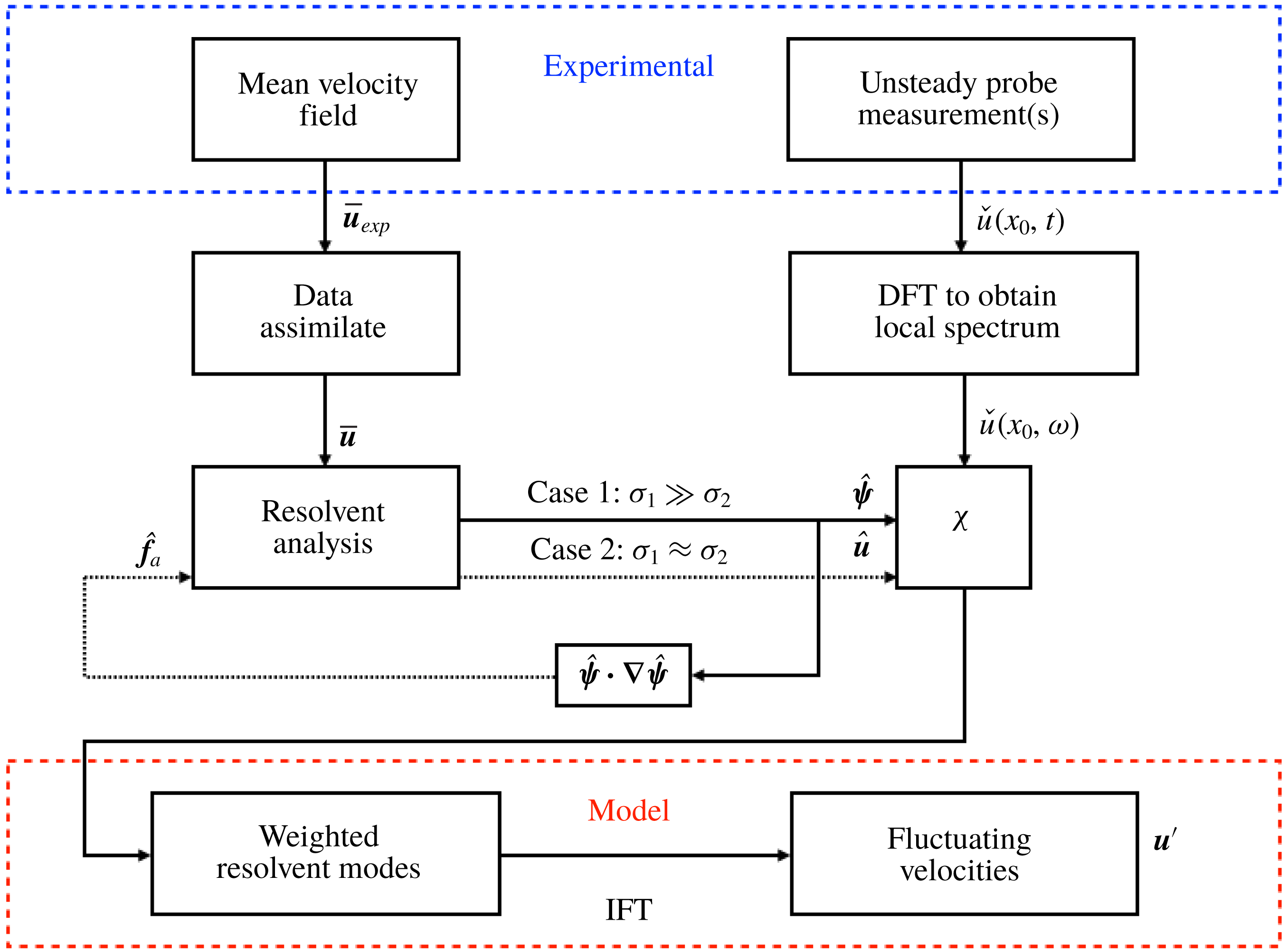
The resolvent-based modelling procedure is summarised in figure 2, which contains the relevant steps starting with the acquisition of the experimental measurements (top row). The mean flow is data assimilated onto a FreeFem mesh with the correct boundary conditions and the time-resolved probe measurements are Fourier transformed in time (row 2). The structure associated with frequency $\unicode[STIX]{x1D714}$ is obtained from resolvent analysis of the data-assimilated mean flow in one of two ways: (i) approximating the operator via the singular value decomposition if $\unicode[STIX]{x1D70E}_{1}\gg \unicode[STIX]{x1D70E}_{2}$ or (ii) approximating the nonlinear forcing if the frequency is energetic but there is no separation of singular values. These two methods are demarcated by solid and dotted lines, respectively, in row 3 of figure 2. The resolvent modes are weighted from the Fourier-transformed probe points and inverse Fourier transformed to obtain a model of the velocity fluctuations in time (bottom row).

Figure 2.

Steps to obtain the resolvent-based model of the velocity fluctuations starting from the experimental measurements, adapted from Symon (Reference Symon2018).

4.1 A0 case

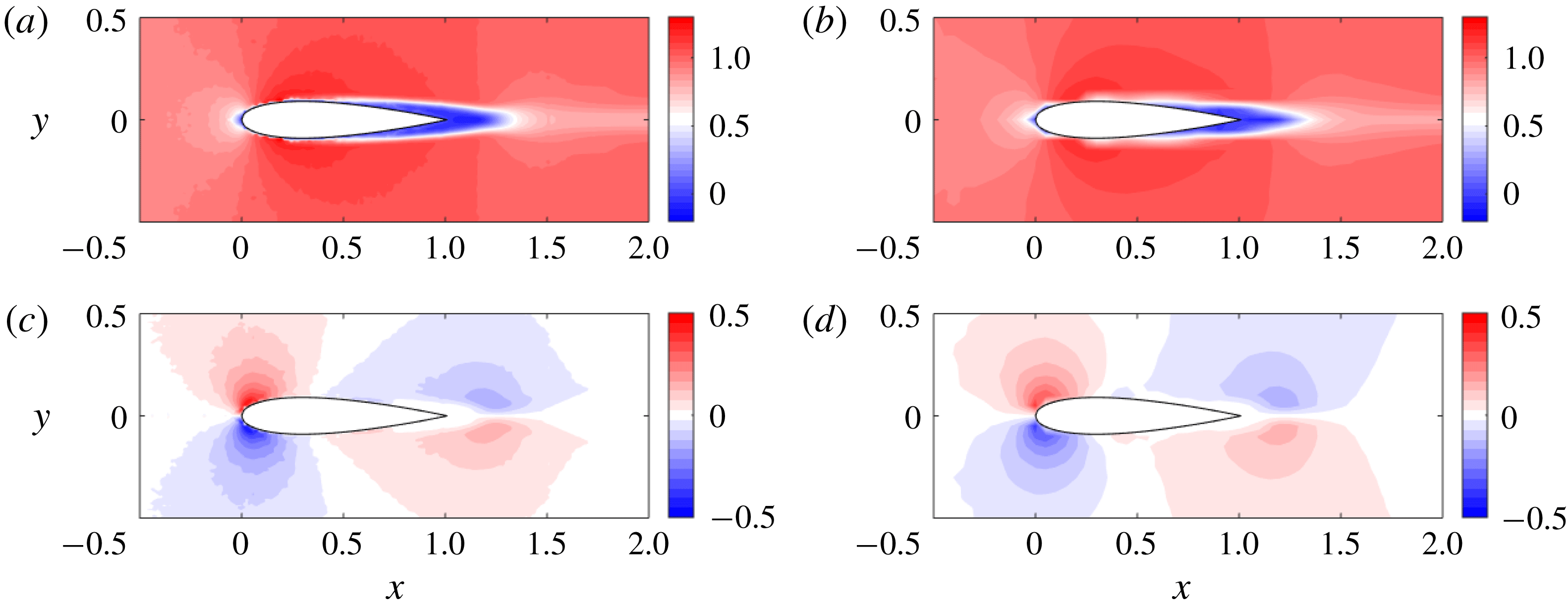
As mentioned in § 2, the data below the airfoil are obstructed by the airfoil’s shadow. To overcome this problem, the data above the centreline are reflected across, keeping the streamwise velocity constant and reversing the sign of the transverse velocity. Both the streamwise and transverse component of the data-assimilated fields are compared to their experimental counterparts in figure 3. The fields are nearly indistinguishable although the data-assimilated contours are slightly more smooth than those in the experiment.

Figure 3.

Data assimilation results for the A0 case. The assimilated velocity fields (b,d) are compared to the experiment (a,c). The streamwise velocity $\overline{u}$ is in the upper row while the transverse velocity $\overline{v}$ is in the lower row.

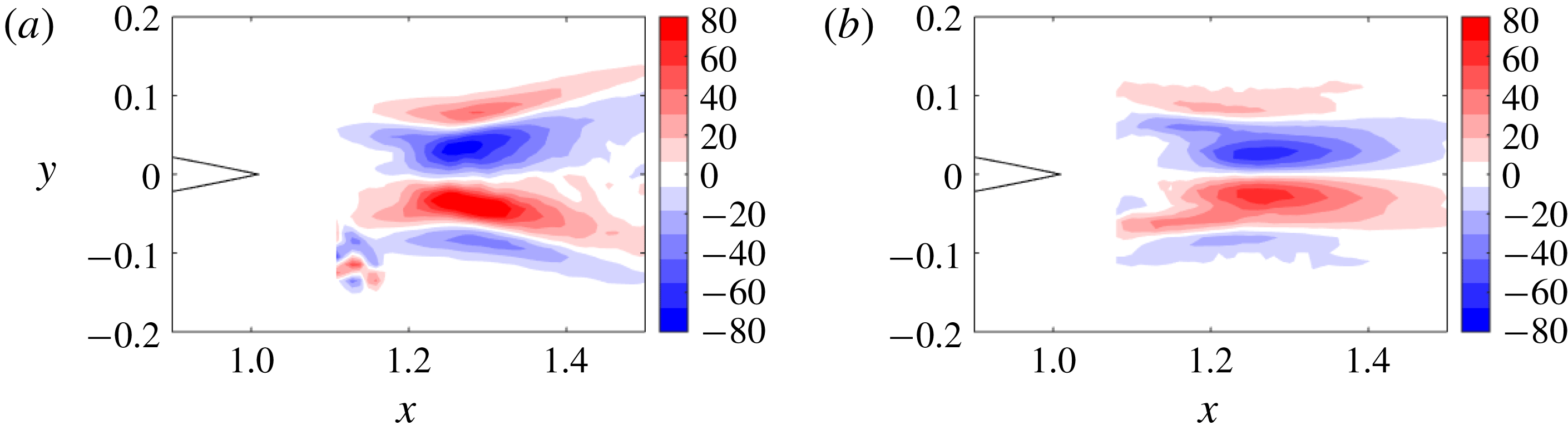
The spanwise component of $\unicode[STIX]{x1D735}\times \boldsymbol{f}$ , rather than $\boldsymbol{f}$ itself, is shown in figure 4 to eliminate the irrotational component which cannot be captured. The agreement between the experimental field, obtained after computing two gradients of the velocity fluctuations, and the data-assimilated field is good despite some minor discrepancies. One notable aspect about figure 4 is that $\unicode[STIX]{x1D735}\times \boldsymbol{f}$ for this flow closely resembles that of cylinder flow (see figures 4 and 5.9 of Foures et al. (Reference Foures, Dovetta, Sipp and Schmid2014) and Symon et al. (Reference Symon, Rosenberg, Dawson and McKeon2018), respectively).

Figure 4.

The spanwise component of $\unicode[STIX]{x1D735}\times \boldsymbol{f}$ from the experiment (a) compared to the data assimilation (b) in the A0 case.

4.2 A10 case

Data assimilation of the A10 case is slightly more difficult since the flow is not symmetric with respect to the centreline. Two separate experiments are conducted at both $\unicode[STIX]{x1D6FC}=-10^{\circ }$ and $\unicode[STIX]{x1D6FC}=10^{\circ }$ . In the first experiment, the data below the airfoil (suction side) are obstructed by the airfoil shadow so only the pressure side can be measured. In the second experiment, the pressure side is obstructed by the shadow, so only the suction side is measured. The final mean velocity field can be obtained by stitching together the two means such that the data around the entire airfoil are known. The stitching process, if imperfect, may result in non-physical measurements although the data-assimilation algorithm is able to compensate for this.

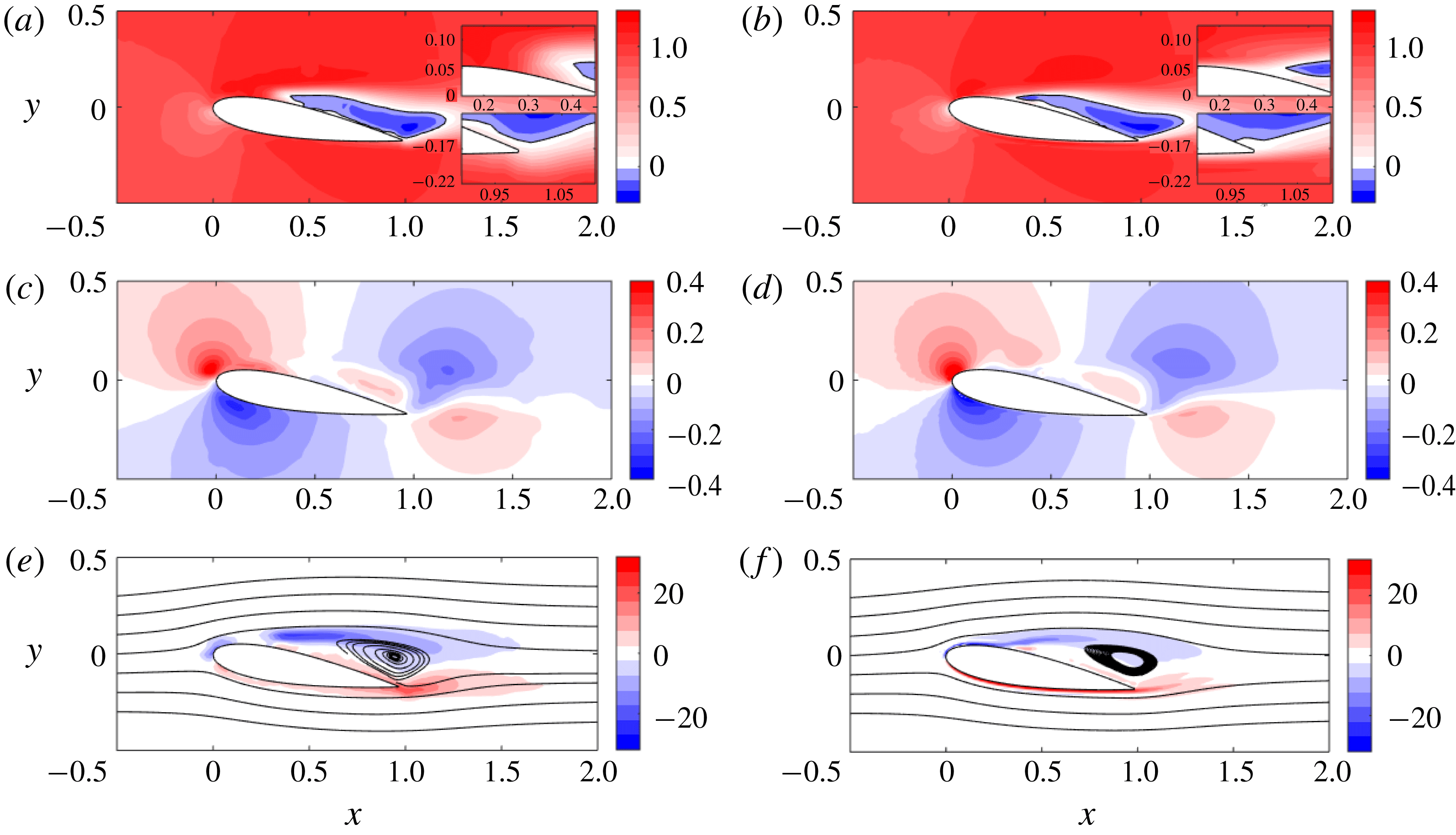
Data assimilation is performed using the stitched mean velocity field, i.e. from measurements at $\unicode[STIX]{x1D6FC}=-10^{\circ }$ and $\unicode[STIX]{x1D6FC}=10^{\circ }$ , and the resulting fields are compared to their experimental counterparts in figure 5. In addition to comparing the two components of the mean velocity field, the mean spanwise vorticity $\overline{\unicode[STIX]{x1D714}}_{z}$ is plotted in the bottom row of figure 5. Streamlines of the mean velocity field indicate the size and location of the recirculation bubble. The streamwise and transverse velocities match very well, particularly with respect to the reverse flow region. The separated flow region is accurately reproduced in the data-assimilated fields.

Figure 5.

Data assimilation results for the A10 case. The assimilated fields (b,d,f) are compared to the experiment (a,c,e): streamwise velocity $\overline{u}$  (a,b), transverse velocity $\overline{v}$  (c,d) and spanwise vorticity $\overline{\unicode[STIX]{x1D714}}_{z}$  (e,f).

There are two regions of the flow field which are visibly improved by data assimilation. The first is near the leading edge of the airfoil, where the flow separates and vortices are formed due to the rollup of the shear layer. This improvement is particularly visible in the vorticity plots since the negative contours of the data-assimilated field are continuous unlike in the experiment where there is a gap at $x\approx 0.2$ . As noted by Raffel et al. (Reference Raffel, Willert, Scarano, Kähler, Wereley and Kompenhans2018), there are difficulties associated with PIV for laminar flow around airfoils. The effects of strong centrifugal forces around the airfoil leading edge and strong shear result in the outward movement of tracer particles in a direction perpendicular to the curved streamlines. This loss of seeding compromises measurements in the region close to the solid body.

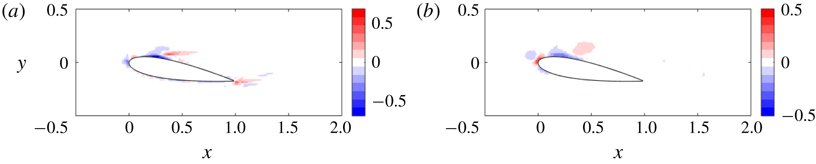
The second area of improvement is at the trailing edge where there are imperfections associated with the stitching together of the two means. Contours of negative mean streamwise velocity protrude below the trailing edge which corresponds to non-physical behaviour. Data assimilation is able to correct this problem and eliminate inaccuracies associated with the stitching process. These changes are more apparent by examining the difference between the assimilated and experimental mean velocities, i.e.  $\unicode[STIX]{x0394}\overline{\boldsymbol{u}}=\overline{\boldsymbol{u}}-\overline{\boldsymbol{u}}_{exp}$ , which is illustrated in figure 6 for both velocity components. The two regions of disagreement, notably, coincide with the areas of improvement discussed earlier.

Figure 6.

Residual discrepancy of the mean streamwise (a) and transverse (b) velocities between the experimental and data-assimilated mean velocity fields.

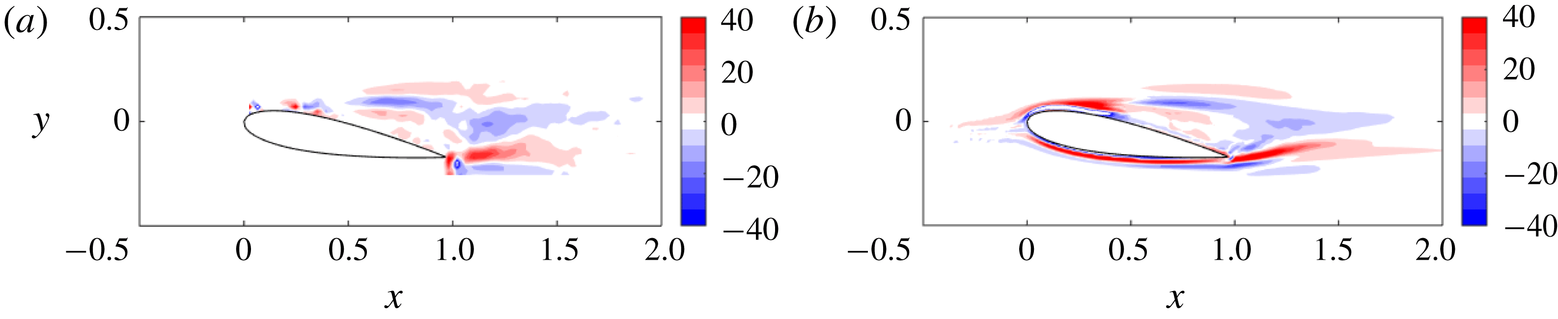
It should be emphasised that the benefit of data assimilating the fields is not only filling in missing data, but also in obtaining gradient quantities with less noise. This is particularly noticeable when comparing the spanwise component of $\unicode[STIX]{x1D735}\times \boldsymbol{f}$ in figure 7. Even though the experimental data do not have much noise to begin with, the data-assimilated field is more smooth overall.

Figure 7.

The spanwise component of $\unicode[STIX]{x1D735}\times \boldsymbol{f}$ from the experiment (a) compared to the data assimilation (b) in the A10 case.

Data assimilation leads to improvement for both the A0 and A10 cases although the changes for A0 are fairly unremarkable. For the A10 case, on the other hand, there are features missing from the experimental mean that data assimilation fills in, particularly at the shear layer originating near the leading edge. As will be seen in § 6, this has major implications for the identification of linear amplification mechanisms in the flow.

5.1 SPOD of the velocity fluctuations

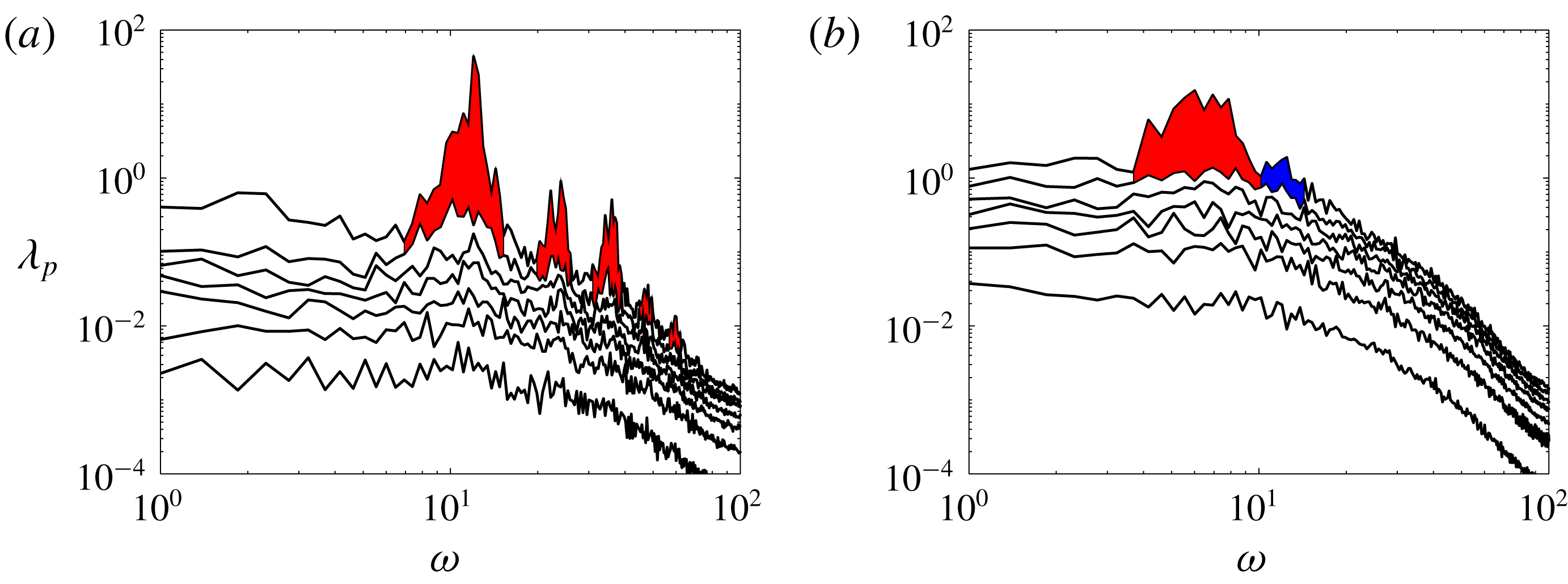
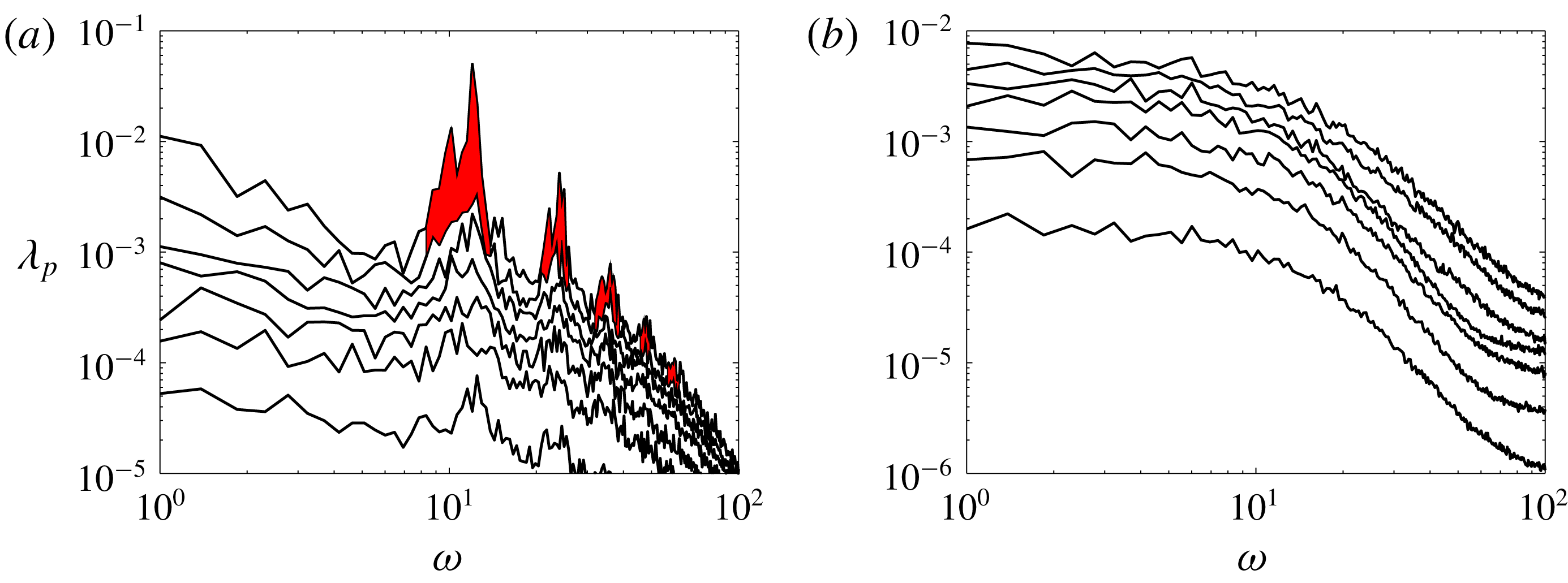
The SPOD eigenspectra for A0 are plotted in figure 8 as a function of $\unicode[STIX]{x1D714}$ . The largest peak in $\unicode[STIX]{x1D706}_{1}$ occurs at $\unicode[STIX]{x1D714}=12.0$ , which corresponds to the shedding frequency of the airfoil. Red patches highlight frequencies at which there is significant separation between the first and second eigenvalues, the former of which exhibits sharp peaks at the shedding frequency and its harmonics.

Figure 8.

The SPOD eigenspectra of the A0 case (a) as a function of $\unicode[STIX]{x1D714}$ where red patches denote frequencies where there is significant separation between the first two eigenvalues. For the A10 case (b), the red patch denotes low-rank behaviour corresponding to the wake dynamics and the blue patch denotes low-rank behaviour corresponding to the shear layer dynamics.

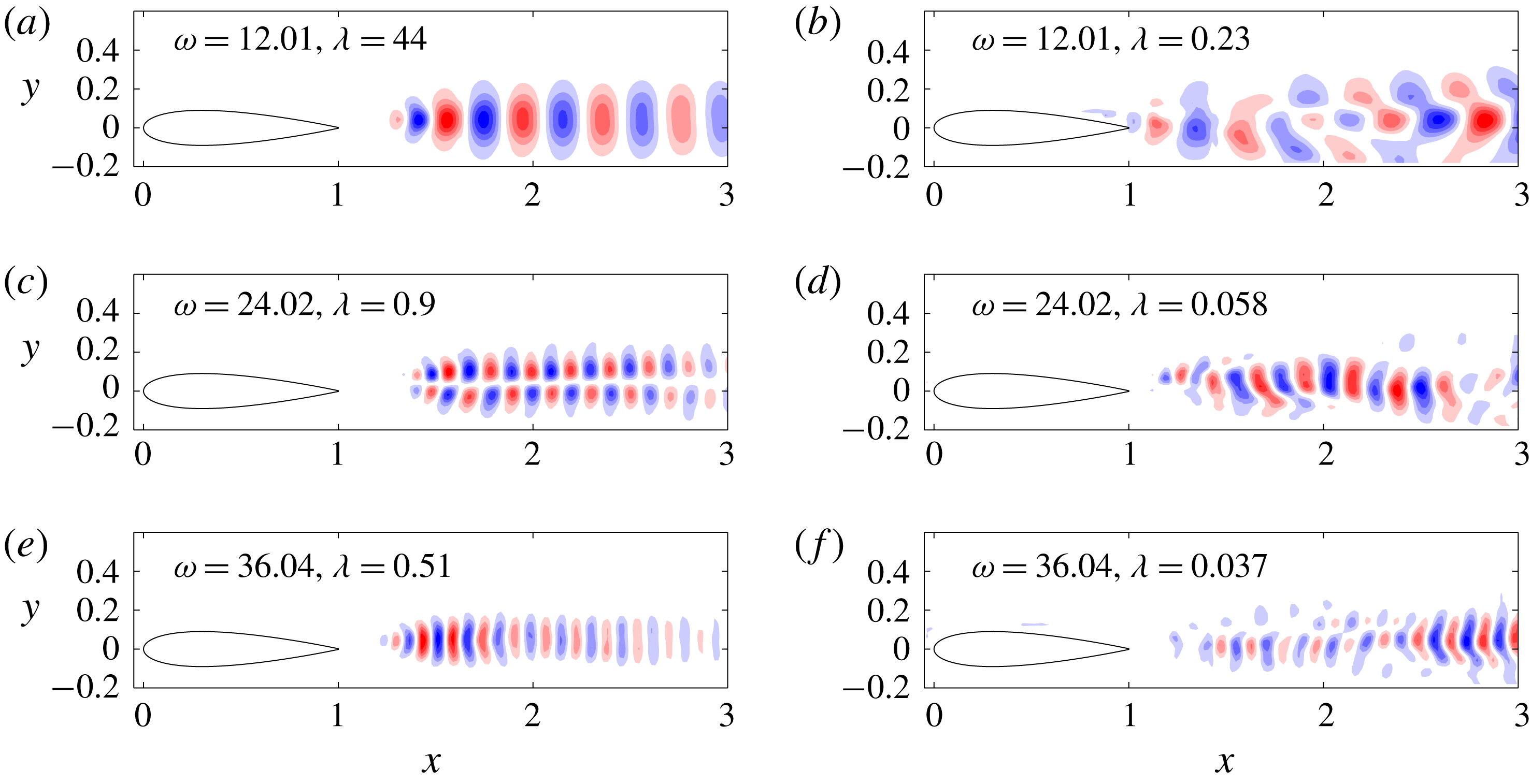
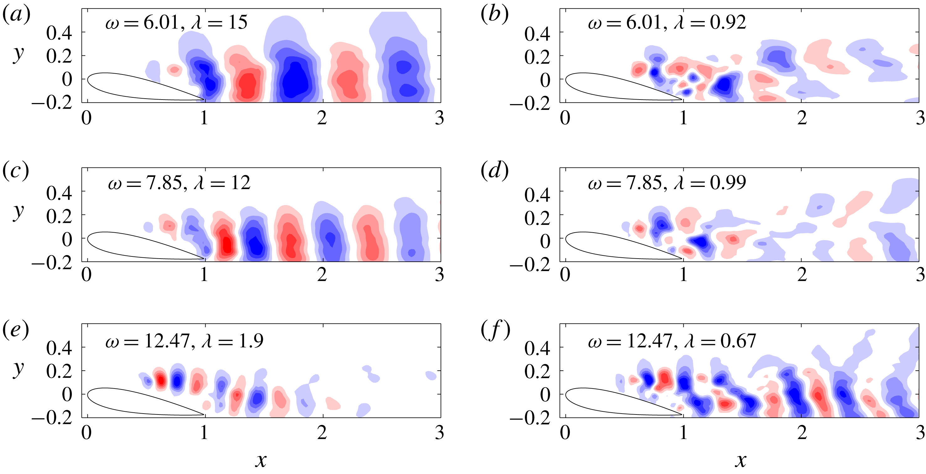
The $v$ -component of the first two SPOD modes is shown in figure 9 for the first three harmonics. In all cases, the first eigenvalue is at least one order of magnitude larger than the second eigenvalue. The first SPOD mode is significantly more structured than the second mode for all three harmonics in figure 9, an observation which is consistent with the fact that nearly all the energy at these frequencies is concentrated in the first mode. For frequencies where $\unicode[STIX]{x1D706}_{1}\approx \unicode[STIX]{x1D706}_{2}$ (not shown in the interest of brevity), the mode shapes are less structured for all eigenvalues.

Figure 9.

The first SPOD mode for the first three harmonics of the shedding frequency (a,c,e) for the A0 case. The second SPOD mode for the first three harmonics of the shedding frequency (b,d,f).

Let us now consider the A10 case. The PIV data are subdivided into the same number of blocks containing the same number of snapshots as in the A0 case to allow for direct comparisons between both angles of attack. The SPOD eigenspectra are plotted in figure 8. It is immediately apparent that the SPOD eigenvalues are far less peaked than they were for the A0 case. Instead of observing a fundamental frequency and its harmonics, there are bands of frequencies where low-rank behaviour can be observed, a feature reminiscent of an amplifier flow. The first region, denoted by the red patch in figure 8, is situated around $4<\unicode[STIX]{x1D714}<8$ while the second one resides roughly between $10.5<\unicode[STIX]{x1D714}<14.5$ .

Figure 10.

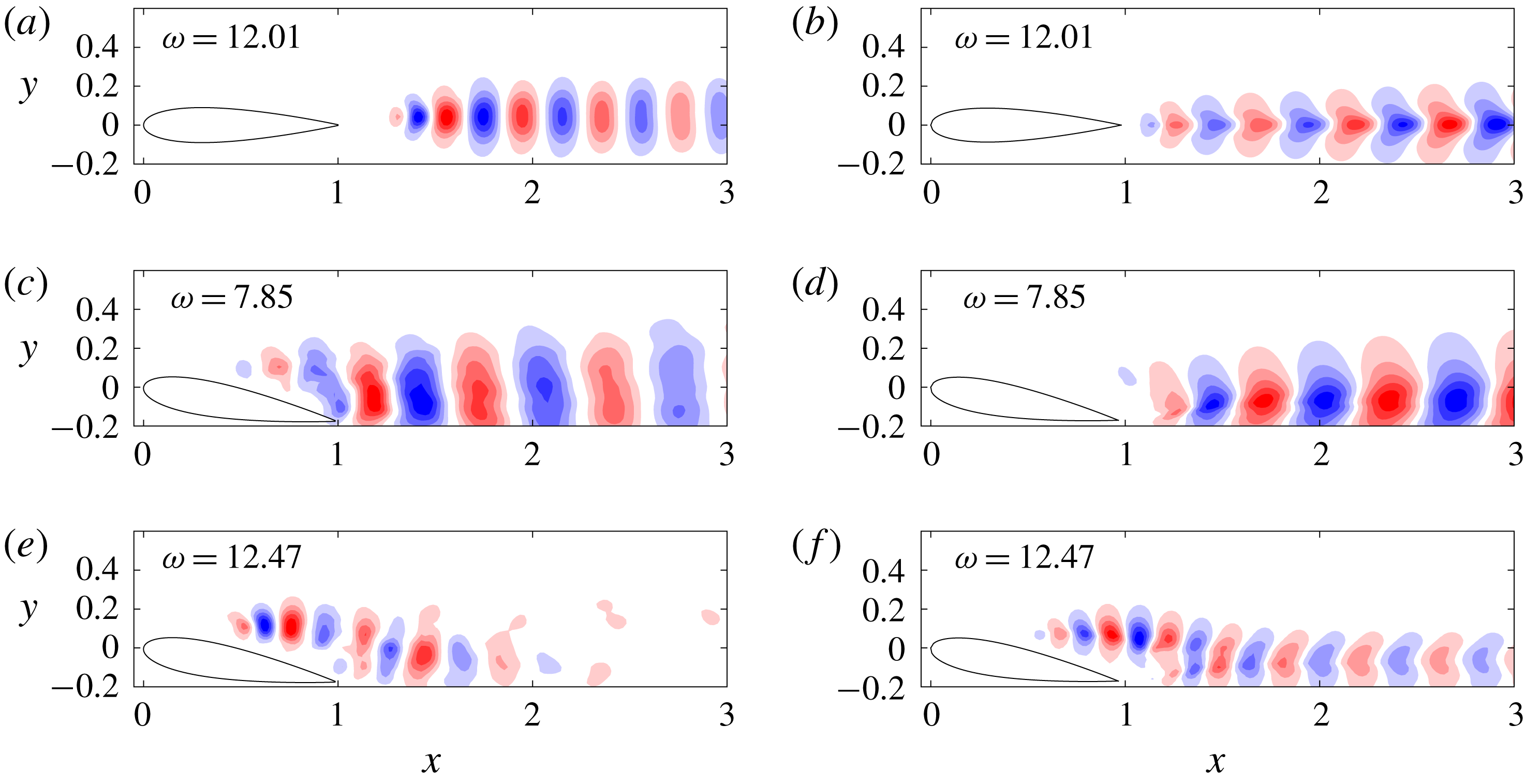
The first SPOD mode for frequencies corresponding to the wake or shear layer dynamics (a,c,e) and the second SPOD mode for the same frequencies (b,d,f) for the A10 case.

The modes for A10 are plotted in figure 10 for the highest eigenvalues in the low- and high-frequency bands. Similar to the A0 case, the leading SPOD mode is highly structured and contains approximately one order of magnitude more energy than the second mode for $\unicode[STIX]{x1D714}=6.01$ and $\unicode[STIX]{x1D714}=7.85$ . Most of the energy in these modes, furthermore, resides in the wake region, or $x>1$ , although there is some structure in the shear layer. The second SPOD mode, on the other hand, is more energetic in the shear layer although it is far less structured. The final frequency considered is $\unicode[STIX]{x1D714}=12.47$ , which is roughly in the middle of the second band of frequencies identified earlier. The first mode is primarily in the shear layer while the second mode resembles a mix of both the shear layer and wake dynamics. Since SPOD takes into consideration the kinetic energy of the entire domain, the SPOD eigenvalues for frequencies corresponding to the shear layer assume lower values. They are dynamically important, nonetheless, since there is non-negligible separation between the first and second eigenvalue. They are also essential to model the fluctuations above the airfoil.

5.2 SPOD of the nonlinear forcing

We now utilise SPOD to characterise the structure of the nonlinear forcing, which is computed from the PIV snapshots since the data are sufficiently well resolved in space and time. The SPOD eigenspectra for both cases (A0 and A10) are plotted together in figure 11 to underscore the contrast between the two cases. The eigenspectra for A0 are still peaked in the sense that the energy is high at the vortex shedding frequency and its harmonics. There is also a considerable gap between the first and second eigenvalues at these frequencies, similar to the trends observed for the velocity fluctuations. The spectra for the A10 case, on the other hand, are relatively flat and have no discernible peaks. The behaviour of the nonlinear forcing bears no resemblance to those of the velocity fluctuations as seen in figure 10.

Figure 11.

SPOD eigenspectra of the nonlinear forcing for the A0 (a) and A10 (b) cases. The red patches in the A0 case delineate the shedding frequency and its harmonics where there is separation between the first and second eigenvalues.

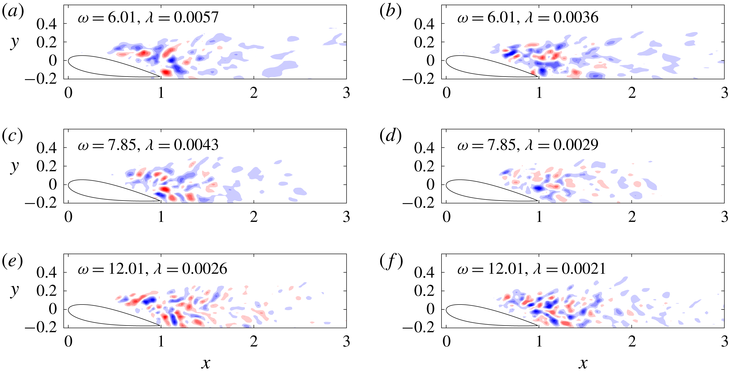
The differences are even more evident when considering the mode shapes. For clarity, we will plot modes at the same frequencies as those in figures 9 and 10 since they are dynamically important. The modes for A0 are plotted in figure 12. It is clear that the nonlinear forcing for the first two harmonics is very structured, as the contours are almost perfectly symmetric (or anti-symmetric in the case of the second harmonic) with respect to the centreline. The structure corresponding to the third harmonic looks slightly more disordered, since it is not particularly energetic, but it can be remarked that the mode shape is approximately symmetric with respect to the centreline and has a well-defined wavelength which is approximately constant, i.e. not changing as a function of $x$ .

Figure 12.

The first (a,c,e) and second (b,d,f) SPOD modes for the nonlinear forcing of the A0 case.

The mode shapes for the A10 case are plotted in figure 12. The results are reminiscent of those from the jet flow study of Towne et al. (Reference Towne, Colonius, Jordan, Cavalieri and Brès2015) in that there is a lack of coherent structure. While there may be some notion of a wavelength associated with these modes, it would be far more difficult to quantify in comparison to the results in figure 12. There is also no noticeable difference between the spatial support of the lower-frequency modes in figure 13 and that of the higher-frequency mode even though the choice of frequency has an impact on the spatial location and distribution of the velocity fluctuations.

Figure 13.

The first (a,c,e) and second (b,d,f) SPOD modes for the nonlinear forcing of the A10 case.

5.3 Discussion and classification of the two cases

SPOD of the velocity fluctuations reveals low-rank behaviour for both the A0 and A10 cases although there are some major differences. The SPOD eigenspectra of A0 are highly peaked at the vortex shedding frequency and its harmonics. The A0 case, thus, can be considered sparse in that there are few energetic frequencies in the flow. The SPOD eigenspectra for A10 are more broadband, with separation between the first and second eigenvalues occurring at two distinct ranges of frequencies making the flow less sparse, i.e. more frequencies are required to model the fluctuating flow field. Within the lower range, the SPOD modes are concentrated in the wake whereas within the higher range, they are concentrated in the shear layer. Based on these trends, the A0 case resembles an oscillator with fluctuations that are characterised by a well-defined frequency. The A10 case behaves more like an amplifier due to the shear layer instability although it can also be characterised as a weak oscillator due to its identifiable shedding frequency.

Application of SPOD to the nonlinear forcing confirms this appraisal. In the case of A0, there is low-rank behaviour at all harmonics and the mode shapes are highly structured as they contain a well-defined wavelength and symmetry. This suggests they can be represented by a limited number of nonlinear interactions whereas in the A10 case, there is no apparent low-rank behaviour and the forcing field contains no coherent structure. These results are consistent with those of Towne et al. (Reference Towne, Colonius, Jordan, Cavalieri and Brès2015) and Rosenberg et al. (Reference Rosenberg, Symon and McKeon2019). It is also in tune with the idea that the input to an amplifier is less important, as the linear dynamics has a preferential bias towards one particular structure.

In theory, this makes modelling of amplifier flows easier as the linear dynamics takes precedence over nonlinearity, which needs to be taken into account for oscillator flows. Consequently, amplifier flows are more amenable to stochastic forcing of an approximated linear operator. Alternatively, the modelling of oscillator flows may benefit from approximating the nonlinear forcing due to the emergence of parasitic modes. These ideas are tested in § 7.

6.1 A0 case: a single linear mechanism

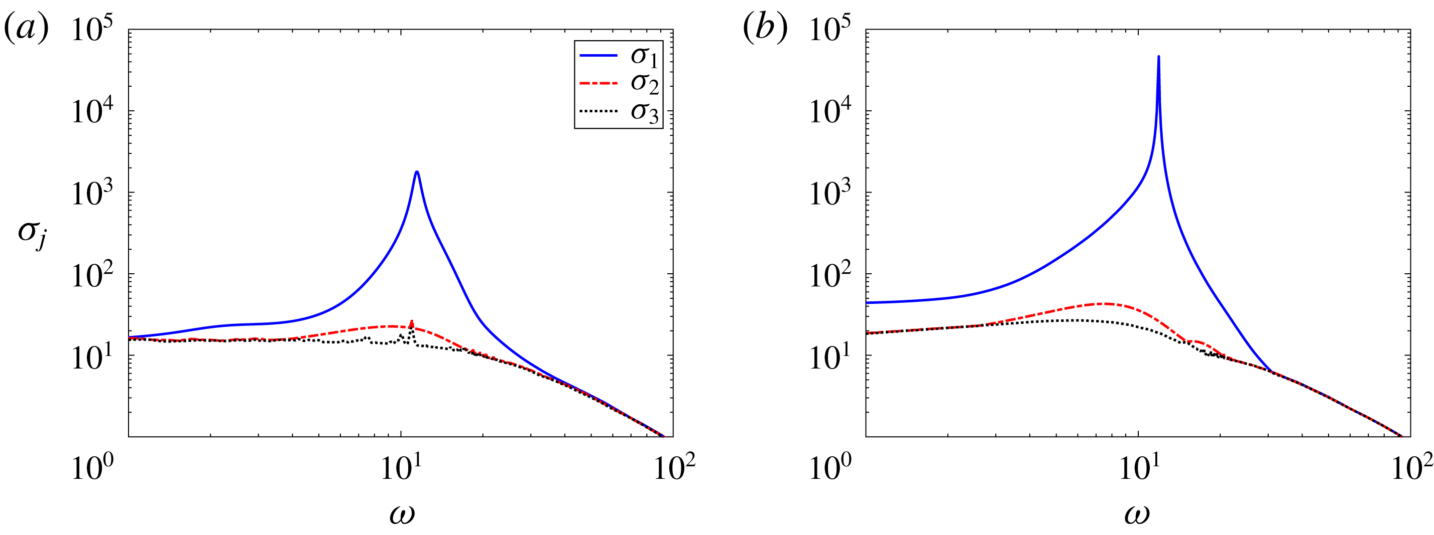
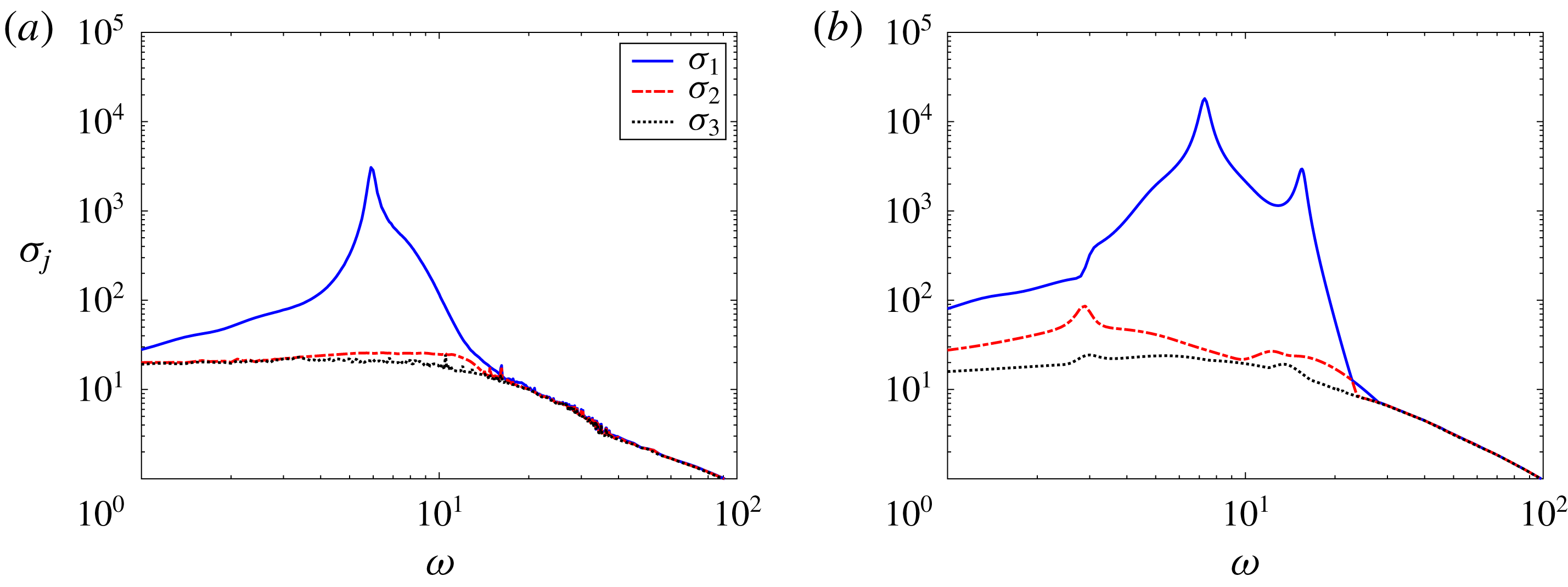
The first three singular values of the resolvent operator are plotted in figure 14 using both the interpolated experimental and data-assimilated means. The trends for both cases are quite similar to cylinder flow (Symon et al. Reference Symon, Rosenberg, Dawson and McKeon2018) in that there is a distinct range of frequencies where the first singular value is an order of magnitude higher than the second singular value. Data assimilating the mean velocity field has a negligible impact on the relative magnitudes of the singular values with respect to one another but it does increase the absolute value of the first singular value near the peak frequency. However, there is no impact on the mode shapes (see Symon Reference Symon2018).

Figure 14.

The first three singular values of the resolvent operator plotted as a function of $\unicode[STIX]{x1D714}$ for the experimental (a) and data-assimilated (b) mean velocity fields of the A0 case.

6.2 A10 case: multiple linear mechanisms

Unlike the A0 case, the singular values, illustrated in figure 15, of the resolvent operator for the A10 case depend strongly on the mean velocity field. The interpolated mean has a single peak at $\unicode[STIX]{x1D714}=5.9$ whereas the data-assimilated mean has two peaks at $\unicode[STIX]{x1D714}=7.3$ and $\unicode[STIX]{x1D714}=15.4$ . The frequency range over which the resolvent is low rank is also much wider for the data-assimilated mean.

Figure 15.

The first three singular values of the resolvent operator plotted as a function of $\unicode[STIX]{x1D714}$ for the experimental (a) and data-assimilated (b) mean velocity fields of the A10 case.

Figure 16.

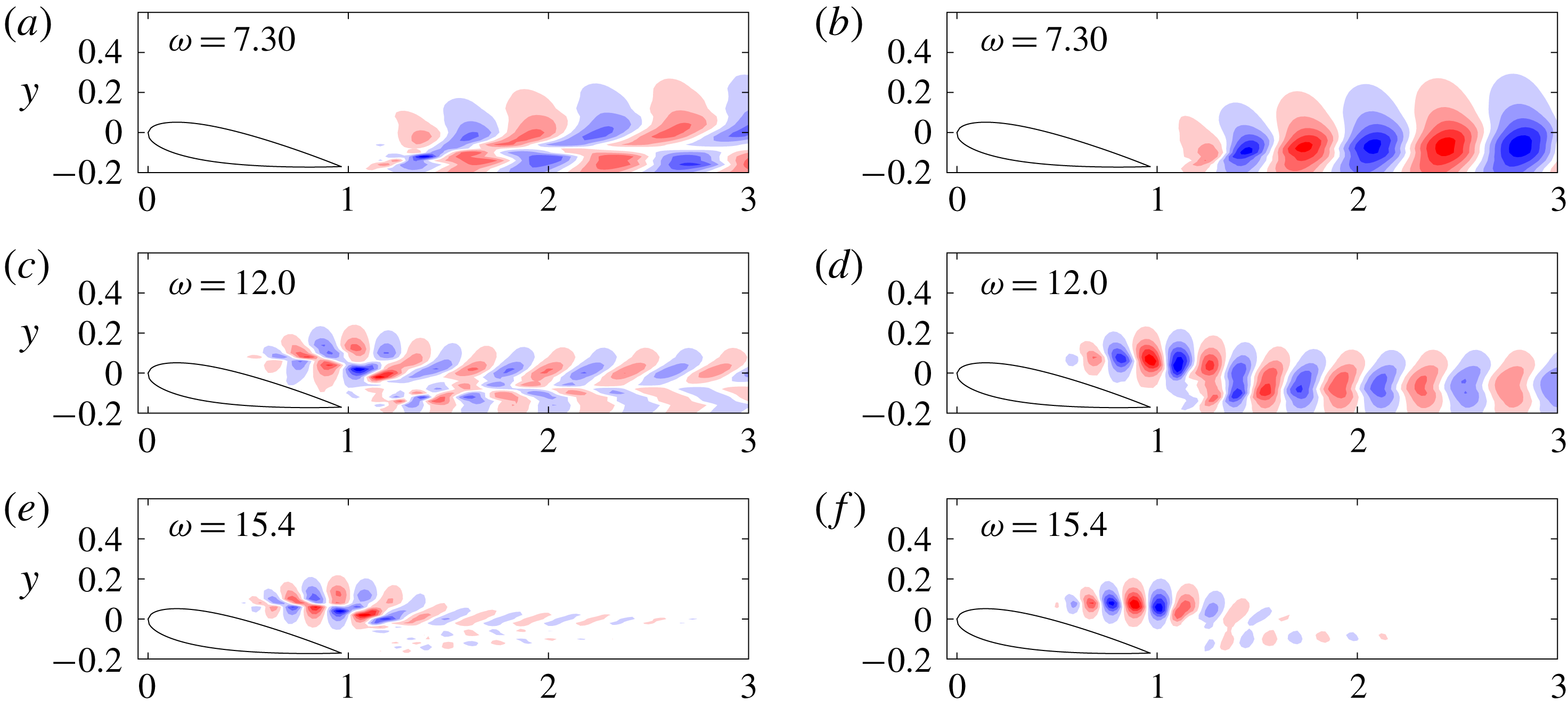
First optimal response mode $\unicode[STIX]{x1D74D}_{1}$ for various frequencies using the A10 data-assimilated mean velocity field. The streamwise and transverse velocity components are plotted in (a,c,e) and (b,d,f), respectively.

The identification of a secondary peak can be attributed to filling in data in the shear layer near the leading edge. As seen in figure 16, which contains the most amplified resolvent mode at two frequencies corresponding to the peaks in figure 15 as well as one intermediate frequency ( $\unicode[STIX]{x1D714}=12.0$ ), two separate linear mechanisms are identified. The first corresponds to shedding- or wake-type modes which occur at lower temporal frequencies (figure 16 a–d). The second corresponds to a Kelvin–Helmholtz instability mechanism in the shear layer which occurs at higher temporal frequencies (figure 16 e,f). The absence of PIV vectors near the leading edge results in resolvent analysis failing to capture the second linear mechanism when the interpolated experimental mean is analysed instead of the data-assimilated mean. The mode shapes for intermediate frequencies have a mix of both linear mechanisms as seen for $\unicode[STIX]{x1D714}=12$ in figure 16. These results are consistent with Thomareis & Papadakis (Reference Thomareis and Papadakis2018) and Yeh & Taira (Reference Yeh and Taira2019), who computed resolvent modes for a NACA 0012 airfoil at similar Reynolds numbers and angles of attack from time-averaged direct numerical simulation (DNS) and large-eddy simulation (LES) data, respectively. The latter study also identified two branches in the eigenspectrum of the LNS operator which were grouped into wake or shear layer modes.

Table 1.

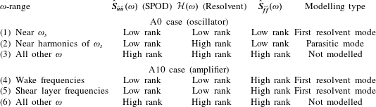
Properties of the cross-spectral density tensors and resolvent operators for the A0 and A10 cases.

6.3 Comparison to SPOD

Even though data assimilation adds no new insight for the A0 case, there are several noteworthy differences between the results of resolvent analysis and SPOD for this flow. The most significant one is that resolvent analysis identifies a single peak at the shedding frequency and low-rank activity is limited to nearby frequencies only. There is no low-rank behaviour at higher harmonics whereas in SPOD, there is an order of magnitude separation between the first and second eigenvalue of the first three harmonics.

These observations can be explained by accounting for the nature of the nonlinear forcing. As in Towne et al. (Reference Towne, Schmidt and Colonius2018), let us rewrite the cross-spectral density at an arbitrary frequency $\unicode[STIX]{x1D714}$ in terms of an expectation operator $\mathbb{E}(\cdot )$ ,

(6.1) $$\begin{eqnarray}\hat{\boldsymbol{S}}_{\hat{\boldsymbol{u}}\hat{\boldsymbol{u}}}(\unicode[STIX]{x1D714})=\mathbb{E}\{\hat{\boldsymbol{u}}(\boldsymbol{x},\unicode[STIX]{x1D714})\hat{\boldsymbol{u}}^{\ast }(\boldsymbol{x},\unicode[STIX]{x1D714})\}.\end{eqnarray}$$

Noting that $\hat{\boldsymbol{u}}(\unicode[STIX]{x1D714})={\mathcal{H}}(\unicode[STIX]{x1D714})\hat{\boldsymbol{f}}(\unicode[STIX]{x1D714})$ , (6.1) can be rewritten as

(6.2) $$\begin{eqnarray}\hat{\boldsymbol{S}}_{\hat{\boldsymbol{u}}\hat{\boldsymbol{u}}}(\unicode[STIX]{x1D714})=\mathbb{E}\{{\mathcal{H}}(\unicode[STIX]{x1D714})\hat{\boldsymbol{f}}(\boldsymbol{x},\unicode[STIX]{x1D714})\hat{\boldsymbol{f}}^{\ast }(\boldsymbol{x},\unicode[STIX]{x1D714}){\mathcal{H}}^{\ast }(\unicode[STIX]{x1D714})\}.\end{eqnarray}$$

Instead of expressing ${\mathcal{H}}(\unicode[STIX]{x1D714})$ in terms of its singular value decomposition, the resolvent operators are moved outside the expectation operator since they are deterministic to yield the following equation:

(6.3) $$\begin{eqnarray}\hat{\boldsymbol{S}}_{\hat{\boldsymbol{u}}\hat{\boldsymbol{u}}}(\unicode[STIX]{x1D714})={\mathcal{H}}(\unicode[STIX]{x1D714})\hat{\boldsymbol{S}}_{\hat{\boldsymbol{f}}\hat{\boldsymbol{f}}}(\unicode[STIX]{x1D714}){\mathcal{H}}^{\ast }(\unicode[STIX]{x1D714}),\end{eqnarray}$$

where $\hat{\boldsymbol{S}}_{\hat{\boldsymbol{f}}\hat{\boldsymbol{f}}}(\unicode[STIX]{x1D714})=\mathbb{E}\{\,\hat{\boldsymbol{f}}(\boldsymbol{x},\unicode[STIX]{x1D714})\hat{\boldsymbol{f}}^{\ast }(\boldsymbol{x},\unicode[STIX]{x1D714})\}$ is the cross-spectral density of the nonlinear forcing as in Towne, Lozano-Durán & Yang (Reference Towne, Lozano-Durán and Yang2019); $\hat{\boldsymbol{S}}_{\hat{\boldsymbol{u}}\hat{\boldsymbol{u}}}(\unicode[STIX]{x1D714})$ may be low-rank in two scenarios.

The first is when the resolvent operator is low rank, which occurs when there is a linear amplification mechanism. This is observed at the shedding frequency of the A0 case, frequencies corresponding to wake modes in the A10 case, and frequencies of the shear layer modes in the A10 case as summarised in rows 1, 4 and 5 in table 1. Both SPOD and resolvent analysis identify low-rank behaviour, similar to the case of the turbulent jet in Schmidt et al. (Reference Schmidt, Towne, Rigas, Colonius and Brès2018) where the Kelvin–Helmholtz instability accounts for the low-rank nature of the cross-spectral density tensor.

The second source of low-rank behaviour can originate from the cross-spectral density of the nonlinear forcing, or $\hat{\boldsymbol{S}}_{\hat{\boldsymbol{f}}\hat{\boldsymbol{f}}}(\unicode[STIX]{x1D714})$ , being low rank. Even if ${\mathcal{H}}(\unicode[STIX]{x1D714})$ is nearly full rank, as it is for higher harmonics of the shedding frequency, the left-hand side of (6.3) will be low rank as long as at least one of the terms on the right-hand side is low rank, i.e.

(6.4) $$\begin{eqnarray}\text{rank}(\hat{\boldsymbol{S}}_{\hat{\boldsymbol{u}}\hat{\boldsymbol{u}}}(\unicode[STIX]{x1D714}))\leqslant \min [\text{rank}({\mathcal{H}}(\unicode[STIX]{x1D714})),\text{rank}(\hat{\boldsymbol{S}}_{\hat{f}\hat{f}}(\unicode[STIX]{x1D714}))].\end{eqnarray}$$

For the A0 case, the nonlinear forcing is very structured at the shedding frequency and its harmonics; consequently, SPOD of the velocity fluctuations reveals large spectral gaps at these frequencies as seen in rows 1 and 2 of table 1. We theorise that the nonlinear forcing can be estimated by limited triadic interactions of resolvent modes to educe the structure at these higher harmonics, a hypothesis which is tested in the next section.

Figure 17.

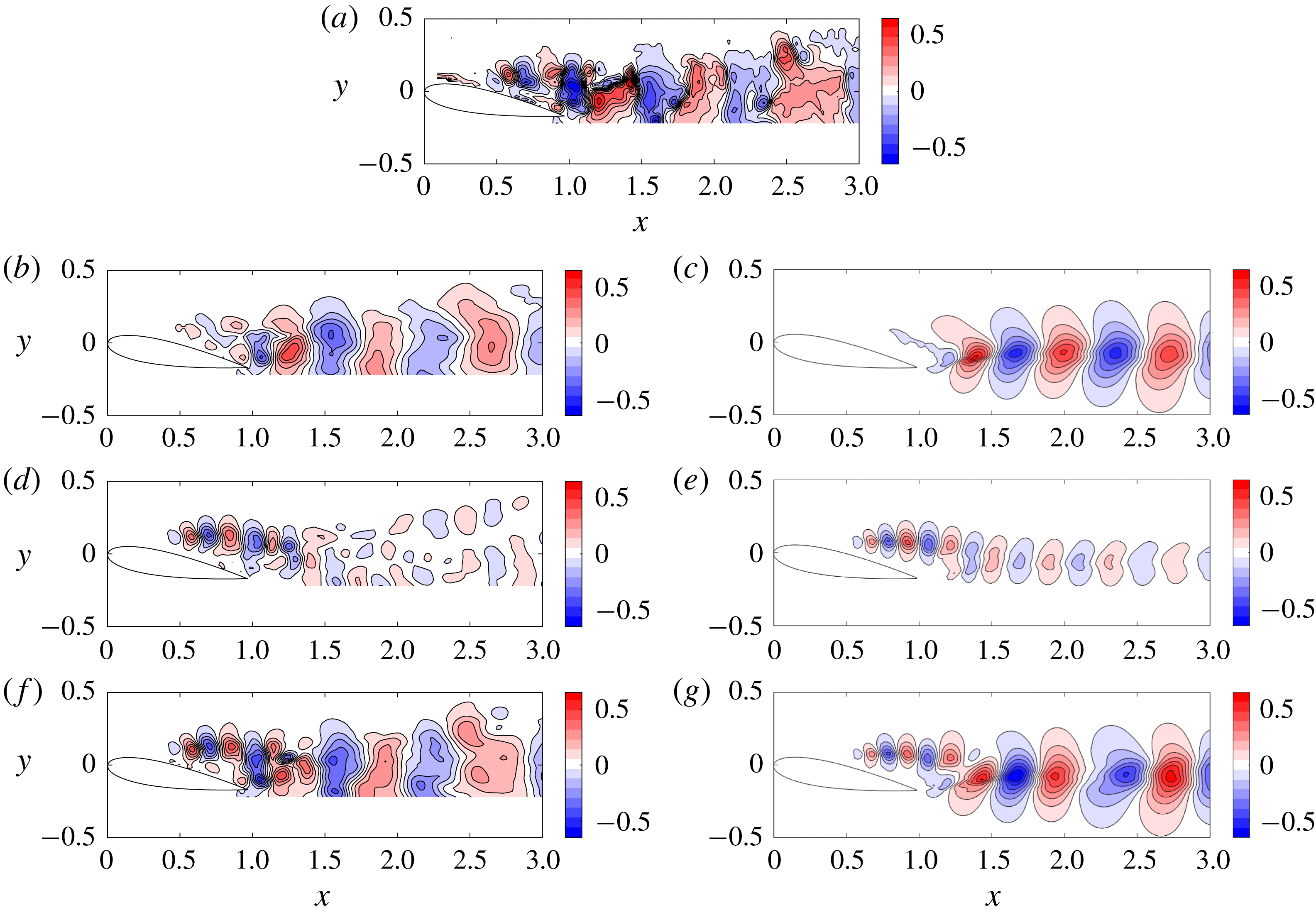
A comparison between the dominant SPOD mode (a,c,e) and the optimal resolvent mode (b,d,f) at highly amplified frequencies.

The SPOD eigenspectra of the nonlinear forcings in figures 12 and 13 verify that the cross-spectral density is low rank at the shedding frequency and its harmonics in the A0 case and at no frequencies for the A10 case. The trends reinforce the notion that A0 behaves like an oscillator while A10 behaves more like an amplifier. It also suggests that resolvent modes and SPOD modes will deviate substantially for the higher harmonics in the A0 case since the resolvent is not low rank and the forcing is anything but white noise in space and time. This will be seen in § 7.1 for the second harmonic of the shedding frequency. The modes for the A10 case, on the other hand, can be expected to match at all frequencies where the resolvent is low rank since these coincide with the low-rank frequencies identified by SPOD.

We compare the dominant SPOD mode to the optimal resolvent mode in figure 17 to reinforce the notion that the first resolvent response mode is representative of the true fluctuations in the flow when the resolvent is low rank. One difference, which is particularly notable for the A0 shedding mode, is that the amplitude of the resolvent mode increases as a function of $x$ . By comparing the final red contour in figure 17(a,b), we note that the amplitude of the SPOD mode is quite weak at $x=2.8$ , whereas it is very strong for the resolvent mode. A similar phenomenon can be observed for the A10 wake mode, which may result from A10 being a weak oscillator. The shear layer mode, on the other hand, is a very close match. Despite these discrepancies, the wavelengths of the modes are in complete agreement, signifying that the resolvent modes correctly predict the convection velocities of the structures in the flow.

7.1 Parasitic modes and modelling of the A0 case

7.1.1 Approximation of the nonlinear forcing

To improve the basis for frequencies outside the range where the resolvent operator is low rank, the nonlinear forcing is approximated using very limited triadic interactions. Let us consider two examples. The simplest is the second harmonic of the shedding frequency $\unicode[STIX]{x1D714}_{s}$ , whose nonlinear forcing is approximated in exactly the same manner as that outlined in Rosenberg et al. (Reference Rosenberg, Symon and McKeon2019), i.e.

(7.1) $$\begin{eqnarray}\hat{\boldsymbol{f}}_{a}(2\unicode[STIX]{x1D714}_{s})\sim \hat{\unicode[STIX]{x1D74D}}_{1}(\unicode[STIX]{x1D714}_{s})\boldsymbol{\cdot }\unicode[STIX]{x1D735}\hat{\unicode[STIX]{x1D74D}}_{1}(\unicode[STIX]{x1D714}_{s}).\end{eqnarray}$$

Many other modes may contribute to the right-hand side of (7.1) although this approximation is adequate since the singular values associated with $\hat{\unicode[STIX]{x1D74D}}_{1}(\unicode[STIX]{x1D714}_{s})$ are very large. Very low frequencies can also be recovered by postulating that they result from the beating of two highly amplified frequencies. The nonlinear forcing for the frequency $\unicode[STIX]{x1D714}=3.70$ , for example, is

(7.2) $$\begin{eqnarray}\hat{\boldsymbol{f}}(\unicode[STIX]{x1D714}=3.70)=-\mathop{\sum }_{\substack{ \unicode[STIX]{x1D714}_{a}+\unicode[STIX]{x1D714}_{b}=3.70 \\ \unicode[STIX]{x1D714}_{a},\unicode[STIX]{x1D714}_{b}\neq 0}}\unicode[STIX]{x1D712}_{1}(\unicode[STIX]{x1D714}_{a})\unicode[STIX]{x1D712}_{1}(\unicode[STIX]{x1D714}_{b})\unicode[STIX]{x1D735}\boldsymbol{\cdot }(\hat{\unicode[STIX]{x1D74D}}_{1}(\unicode[STIX]{x1D714}_{a})\hat{\unicode[STIX]{x1D74D}}_{1}^{T}(\unicode[STIX]{x1D714}_{b})).\end{eqnarray}$$

Since the singular value associated with the shedding frequency at $\unicode[STIX]{x1D714}_{s}=12.0$ is very large, it can be reasoned that the magnitude of $\unicode[STIX]{x1D712}_{1}$ for this frequency will outweigh all other terms in (7.2). To obtain the correct frequency, therefore, it only needs to interact with the frequency $\unicode[STIX]{x1D714}=-8.30$ , where the resolvent operator is still approximately rank-1, to produce a mode at the desired frequency $\unicode[STIX]{x1D714}=+3.70$ . Equation (7.2), therefore, reduces to

(7.3) $$\begin{eqnarray}\hat{\boldsymbol{f}}_{a}(\unicode[STIX]{x1D714}=3.70)\sim \hat{\unicode[STIX]{x1D74D}}_{1}(\unicode[STIX]{x1D714}=12.0)\boldsymbol{\cdot }\unicode[STIX]{x1D735}\hat{\unicode[STIX]{x1D74D}}_{1}(\unicode[STIX]{x1D714}=-8.30)+\hat{\unicode[STIX]{x1D74D}}_{1}(\unicode[STIX]{x1D714}=-8.30)\boldsymbol{\cdot }\unicode[STIX]{x1D735}\hat{\unicode[STIX]{x1D74D}}_{1}(\unicode[STIX]{x1D714}=12.0),\end{eqnarray}$$

where the $\unicode[STIX]{x1D712}_{1}$ terms have been dropped since $\unicode[STIX]{x1D712}_{1}(\unicode[STIX]{x1D714}=12.0)\unicode[STIX]{x1D712}_{1}(\unicode[STIX]{x1D714}=-8.3)$ appears before each term in (7.3) and, at this point, we are only interested in improving the basis for this particular frequency. If we were to include more triads in either (7.1) or (7.3), we would need to know the phase of the modes since $\unicode[STIX]{x1D712}_{1}$ appears before each mode in (7.2). We argue here that the high amplifications associated with the shedding mode allow us to ignore the triadic interactions of suboptimal modes and frequencies which are less amplified.

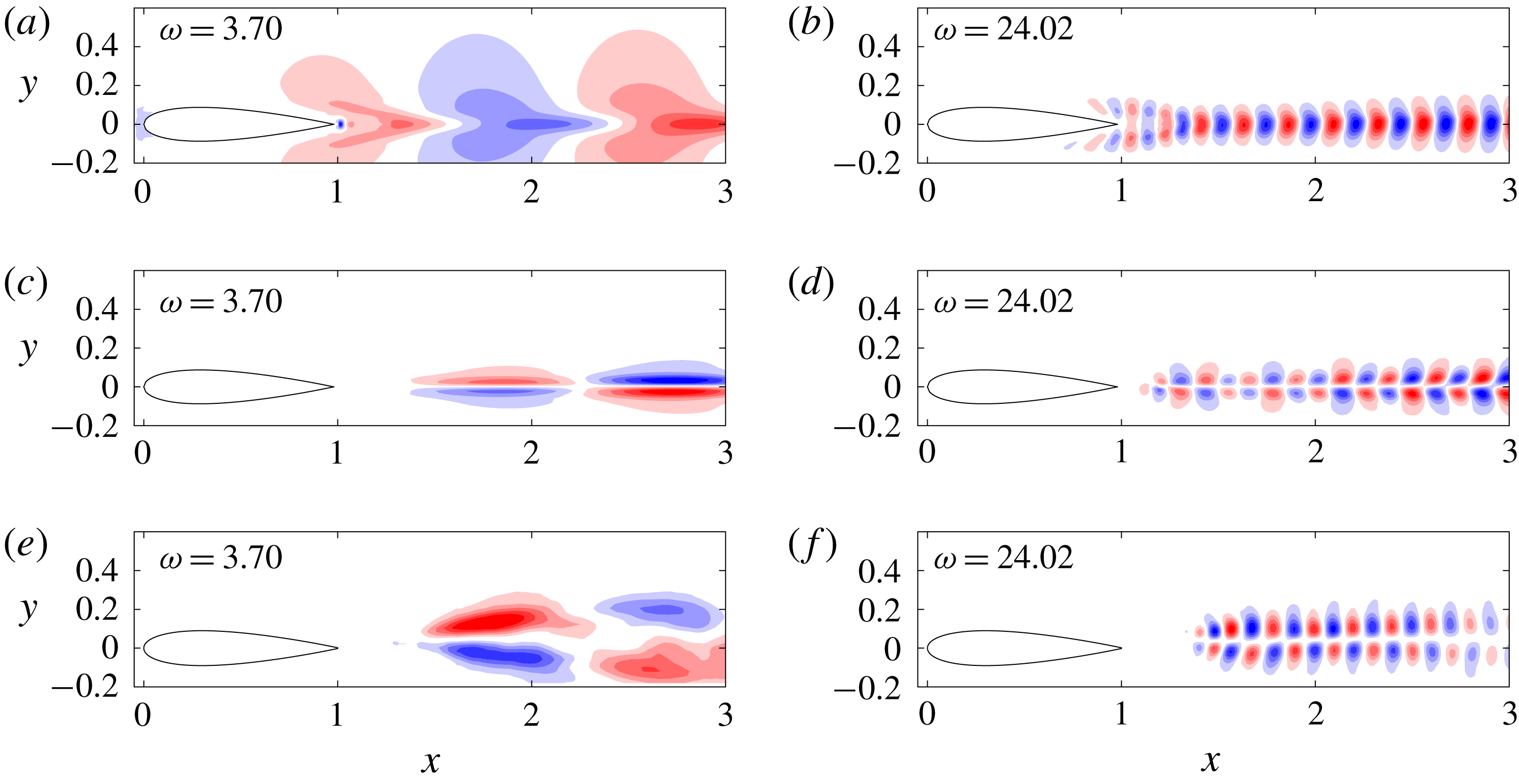
The parasitic modes, or ‘forced’ resolvent modes (i.e. those obtained after right multiplying the resolvent operator by the approximated nonlinear forcing), are compared to the optimal response mode $\hat{\unicode[STIX]{x1D74D}}_{1}$ from the singular value decomposition and the first SPOD mode in figure 18. Despite how simple the modelling for the nonlinear forcing is, the structure at all frequencies considered is a major improvement over the predicted structure from the first resolvent response mode. In particular, the parasitic mode obeys the correct symmetries while the optimal response mode resembles a stretched or compressed version of the vortex shedding mode.

Figure 18.

The optimal response mode (a,b) compared to the parasitic mode (c,d) and the first SPOD mode (e,f).

7.1.2 Modelling preliminaries

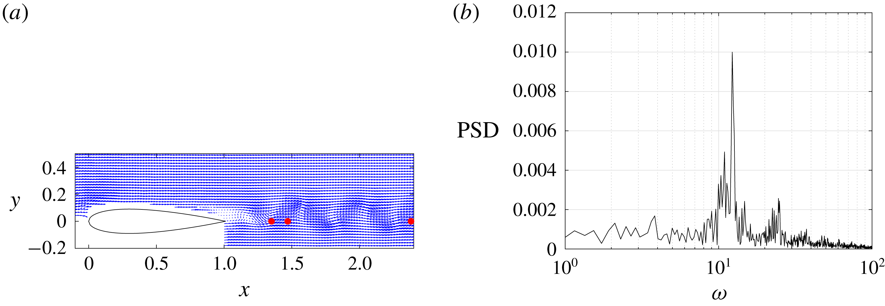
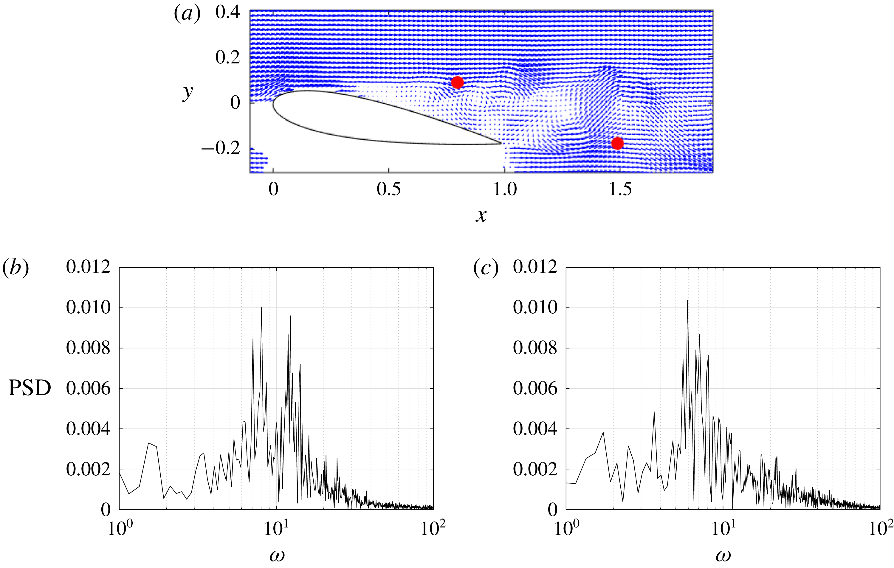
Several candidate points to calibrate the complex weights of the resolvent modes are displayed in figure 19. They are referred to as points 1, 2 and 3, and are ordered by their streamwise position, i.e. point 1 is the furthest upstream. The power spectrum of P2 (P1 and P3 are very similar) for the transverse velocity component, plotted in figure 19, contains a large peak at $\unicode[STIX]{x1D714}=12.0$ and a secondary one at $\unicode[STIX]{x1D714}=24.0$ . These are the first and second harmonics of the shedding frequency, respectively. There is another discernible peak at $\unicode[STIX]{x1D714}=10.7$ resulting from jitter in the shedding frequency. This is also present in the SPOD results for the leading eigenvalue, although it is less noticeable. The jitter does not influence the resolvent norm.

Figure 19.

Candidate probe points (a) and the power spectrum of $\check{v}(t)$ for P2 (b).

Table 2.

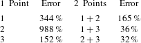
Error for the A0 case as a function of point selection.

The unweighted resolvent modes are first normalised using the standard energy inner product based on the two velocity components. Once the resolvent modes are weighted using the calibration point, they should reflect the true magnitude of the fluctuations. To make a fair comparison between the model and snapshots obtained from PIV, the experimental data are filtered to exclude temporal frequencies outside the range used in the model. The filtering involves Fourier transforming the raw PIV data in time, truncating Fourier modes at unwanted frequencies and inverse Fourier transforming back into the time domain. Another possible way to compare the resolvent model to the experiment is to project the raw data onto the first SPOD mode at all frequencies of interest. Generally these would be where SPOD is approximately rank-1. Since the frequency resolution of the SPOD modes is only $\unicode[STIX]{x0394}\unicode[STIX]{x1D714}\approx 0.5$ , we choose to filter based on the first procedure.

7.1.3 Results and quantification of error

We begin by comparing the performance of each candidate point. The instantaneous error is computed between the model and PIV as follows:

(7.4) $$\begin{eqnarray}I_{v}(t)=\sqrt{\mathop{\sum }_{i=1}^{N}(v^{i}(t)-v_{PIV}^{i}(t))^{2}},\end{eqnarray}$$

where $v$ denotes the transverse velocity component and $N$ is the number of PIV vectors; $I_{v}(t)$ is integrated in time to obtain a global error metric

(7.5) $$\begin{eqnarray}E_{v}=\sqrt{\left(\frac{1}{T}\int _{0}^{T}I(t)^{2}\,\text{d}t\right)}.\end{eqnarray}$$

Here, $E_{v}$ is normalised by the total kinetic energy contained in the filtered PIV and the results for each point are summarised in table 2. Even though the performance of each point is good at some time instants, the overall performance for all three is relatively poor although P3 is the best. If two points are considered, the performance is nearly an order of magnitude better. Furthermore, points which are situated further downstream in the flow yield better results, which is a consequence of the resolvent modes failing to capture the correct streamwise decay of the fluctuations. The combination of points P2 and P3 yields the lowest amount of error, so the following discussion considers this choice only.

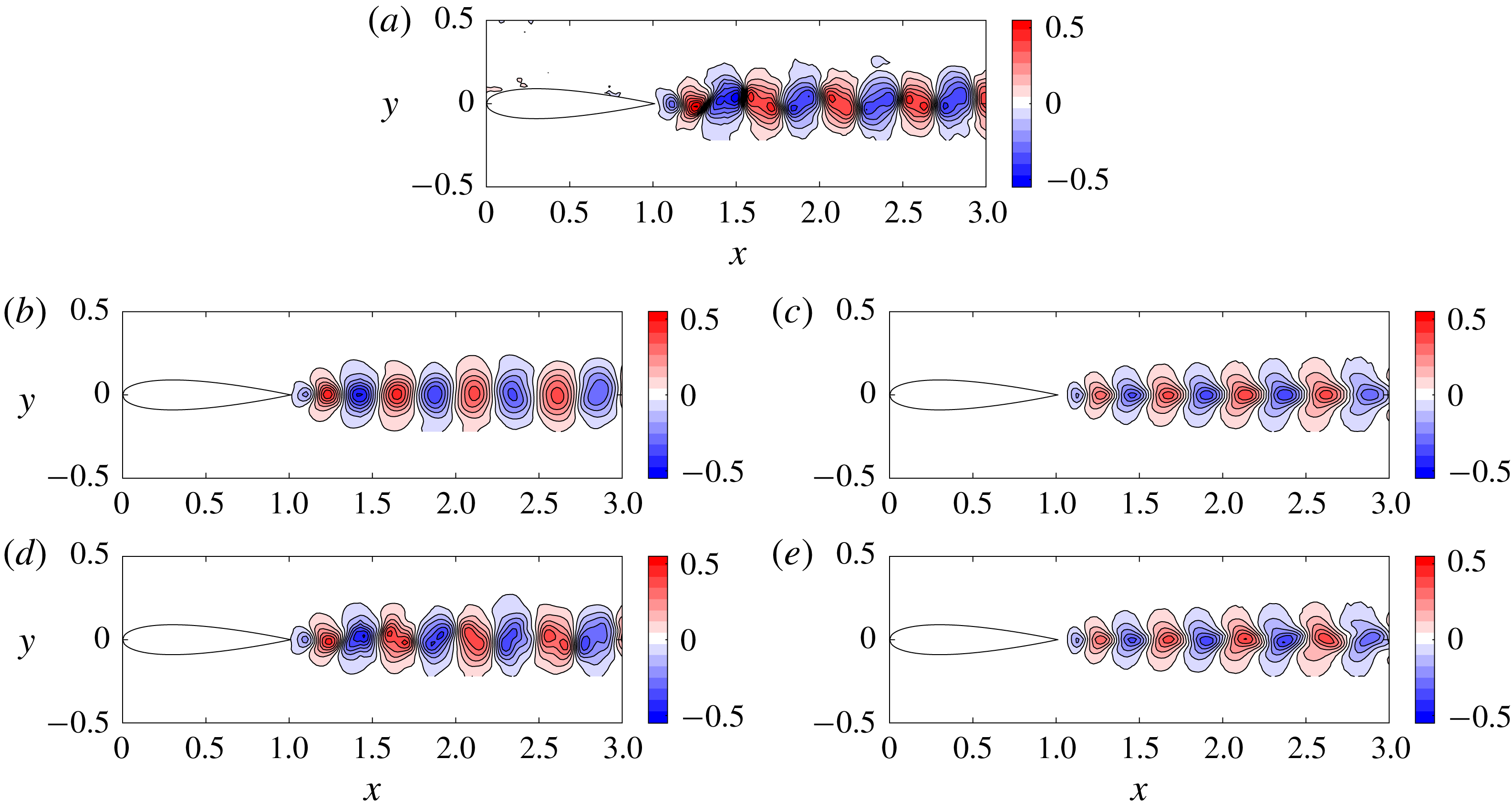
The values computed in table 2 factor in all resolvent modes computed, i.e. both classical and parasitic. The first modelling attempt, however, only uses modes where the resolvent operator is nearly rank-1, i.e.  $6.73<\unicode[STIX]{x1D714}<15.7$ , henceforth referred to as rank-1 modes. These 41 modes are computed using the first singular response mode of the resolvent operator. Harmonics of the shedding frequency where SPOD reveals low-rank behaviour are excluded for now. A representative snapshot is presented in figure 20 and the flow resembles the traditional von Kármán vortex street behind a cylinder. The raw PIV data are contained in the top row while the filtered PIV are compared to the resolvent model using rank-1 modes only in the second row.

Figure 20.

A0 results: (a) the unfiltered PIV snapshot. (b,c) Filtered PIV containing frequencies $6.73<\unicode[STIX]{x1D714}<15.7$ compared to the resolvent model. (d,e) Filtered PIV containing $\unicode[STIX]{x1D714}<39$ compared to the resolvent model.

The velocity fluctuations are symmetric with respect to the centreline since the most amplified structure predicted by resolvent analysis resembles the von Kármán vortex street at all rank-1 frequencies. Similar to the cylinder, there is only one linear mechanism, so modes at suboptimal frequencies end up being a stretched or compressed (in the streamwise direction) version of the shedding mode (see Symon Reference Symon2018; Symon et al. Reference Symon, Sipp, Schmid and McKeon2019). The true velocity fluctuations are not symmetric with respect to the centreline if all frequencies are considered. The difference between the filtered PIV and resolvent model is plotted in figure 21. The largest discrepancies occur immediately behind the trailing edge ( $1.0<x<1.5$ ), where the fluctuations are under predicted by the resolvent model. By calibrating at points P2 and P3, where the resolvent modes over predict the fluctuations, the resulting model has a harder time reconstructing the region further upstream.

Figure 21.

The discrepancy between the filtered PIV and the resolvent model using rank-1 frequencies only (a) and with the inclusion of parasitic modes (b).

When parasitic modes are included, the model is no longer constrained to be symmetric since the second harmonic and low-frequency modes are antisymmetric with respect to the centreline. The flow is now modelled using 91 modes ranging from frequencies as low as $\unicode[STIX]{x1D714}=2.72$ to frequencies as high as $\unicode[STIX]{x1D714}=39$ , in order to encompass the third harmonic. The resolvent model is animated in time and compared to the filtered PIV in movies 1 and 2, respectively, available at https://doi.org/10.1017/jfm.2019.747. Not all frequencies within this range are included since many of them are not energetic as indicated by the probe points. The model is compared to the filtered PIV in figure 20(d,e).

Because the modes outside the rank-1 range are not particularly energetic, the filtered PIV in the bottom row resembles the raw PIV snapshot in the top row fairly well (it contains 80 % of the kinetic energy). The addition of parasitic modes does not dramatically improve the model, but it does capture more detailed features of the flow field. Further downstream, the negative velocity perturbations tilt upstream while the positive velocity perturbations tilt downstream and this is consistent with the PIV data. The discrepancy between the improved model and the filtered PIV is illustrated in figure 21. Small improvements can be seen in the region beyond $x=1.5$ . For this particular snapshot, the addition of parasitic modes reduces the error from 22 % to 18 %.

7.2 Two linear mechanisms and modelling of the A10 case

7.2.1 Selection of probe points

The challenge associated with the A0 case was to incorporate parasitic modes using nonlinear interactions. For the A10 case, the difficulty stems from being able to capture the two linear mechanisms present in the flow. Two candidate points are proposed in figure 22. P4 is located in the shear layer and P5 is in the airfoil wake. The power spectrum for P4 contains two broad peaks at frequencies similar to those identified by resolvent analysis and SPOD. This strengthens the argument that the resolvent tends to be low rank at energetic frequencies as remarked by Moarref et al. (Reference Moarref, Sharma, Tropp and McKeon2013) for wall-bounded turbulent flows. The power spectrum for P5, on the other hand, contains one broad peak centred around the wake frequencies. It seems reasonable, therefore, to suggest that calibrating the modes using this point alone would not successfully model the fluctuations in the shear layer.

Figure 22.

(a) Probe points P4 and P5 in the shear layer and wake, respectively, and their power spectra (b,c) for the A10 case.

The performance using a single point or both points is summarised in table 3 using 66 modes in the range $3.14<\unicode[STIX]{x1D714}<17.7$ . The reconstruction does very badly when only P4 is used as it overpredicts the fluctuations in the wake substantially. P5 is an improvement but it underpredicts the fluctuations in the shear layer. The model performs best when both points are used to calibrate the resolvent modes.

Table 3.

Error for the A10 case as a function of point selection.

7.2.2 Modelling of the A10 velocity fluctuations

For the sake of brevity, only results for the use of both points are summarised in figure 23 as they help explain why a single point is not sufficient to obtain a good model of the flow. The raw PIV data are visualised in the top row. It is fairly evident that the flow is more complicated for this angle of attack as the presence of both linear mechanisms can be observed in relatively distinct regions of the flow. There is also an area immediately behind the trailing edge where they overlap leading to more complex flow structures.

Similar to the A0 case, the PIV data are frequency filtered. We begin by considering 31 frequencies where roughly wake modes only are present, i.e.  $3.15<\unicode[STIX]{x1D714}<9.65$ , as seen in figure 23(b,c). Even though there is some activity in the shear layer, it is small in comparison to the unfiltered case. The resolvent model is plotted alongside it. While the agreement between the wavelengths of the structures is excellent, the model overpredicts the intensity of the fluctuations as far upstream as $x=1.5$ .

Figure 23.

A10 results: (a) the unfiltered PIV snapshot. (b,c) Filtered PIV containing frequencies $3.14<\unicode[STIX]{x1D714}<9.88$ compared to the resolvent model. (d,e) Filtered PIV containing $11.0<\unicode[STIX]{x1D714}<17.7$ compared to the resolvent model. (f,g) Filtered PIV containing $3.14<\unicode[STIX]{x1D714}<17.7$ compared to the resolvent model.

The PIV data are next filtered to retain 31 frequencies corresponding to the shear layer dynamics, i.e.  $11.0<\unicode[STIX]{x1D714}<17.7$ , and are compared to the resolvent model in figure 23(d,e). The model is very good, both in terms of the wavelengths of the structures predicted and their amplitudes. The signature of these modes at P5 is almost negligible, however, so the model misses them altogether when only P5 is considered. This explains why the use of two points fares significantly better than just one.

Finally, the model is compared to the filtered PIV for $3.14<\unicode[STIX]{x1D714}<17.7$ (all 66 frequencies) in the figure 23(f,g). Consistent with earlier results, the agreement is best in the shear layer while the performance of the model degrades further downstream. The model does capture some of the complex behaviour immediately behind the airfoil and the inclination of the fluctuations is correct overall. Despite poor performance further downstream, potential reasons for which are discussed in the next subsection, the resolvent model does quite well at reproducing the coherent structures of the flow.

7.3 Experimental limitations

Before we conclude, we discuss how the results could be improved and why this is difficult to achieve due to the limitations of the current experimental data sets.

The main problem associated with both cases is that the resolvent modes do not correctly model the streamwise decay of the fluctuations, a phenomenon also remarked upon by Rosenberg et al. (Reference Rosenberg, Symon and McKeon2019) for cylinder flow. In order to combat this problem, Rosenberg et al. (Reference Rosenberg, Symon and McKeon2019) approximated the nonlinear forcing for the shedding frequency using the triadic interaction between the shedding mode, predicted by the singular value decomposition, and the parasitic mode at the second harmonic, i.e.

(7.6) $$\begin{eqnarray}\hat{\boldsymbol{f}}_{a}(\unicode[STIX]{x1D714}_{s})\sim \hat{\unicode[STIX]{x1D74D}}_{1}(-\unicode[STIX]{x1D714}_{s})\boldsymbol{\cdot }\unicode[STIX]{x1D735}\hat{\boldsymbol{u}}_{a}(2\unicode[STIX]{x1D714}_{s})+\hat{\boldsymbol{u}}_{a}(2\unicode[STIX]{x1D714}_{s})\boldsymbol{\cdot }\unicode[STIX]{x1D735}\hat{\unicode[STIX]{x1D74D}}_{1}(-\unicode[STIX]{x1D714}_{s}).\end{eqnarray}$$

We attempted to do the same for the A0 and A10 cases since we have a good prediction of the fluctuation at the shedding frequency from the optimal resolvent mode and the second harmonic by approximating its nonlinear forcing. SPOD of the nonlinear forcing, furthermore, strongly suggests that it is necessary to account for this feedback since there is separation between the first two SPOD eigenvalues and the first mode is very structured. The approximated nonlinear forcing for the airfoil at the shedding frequency, however, did not improve the mode shape.

A possible reason for why this failed might be related to the enormous amplification at the shedding frequency due to the proximity of a stable eigenvalue to the neutral axis. Similar to cylinder flow, it is necessary to obtain a very accurate estimate of the nonlinear forcing in order to obtain the correct mode since the resolvent operator is so biased in favour of the first response mode. Lesshafft et al. (Reference Lesshafft, Semeraro, Jaunet, Cavalieri and Jordan2019) also remarked that spurious numerical noise can be sufficient to trigger the optimal mode and thus overwhelm suboptimal modes. The data-assimilated mean is not completely free of noise so the resolvent modes and their triadic interactions are not sufficiently accurate to alter the mode shape predicted by the resolvent at the shedding frequency. As such, an eddy viscosity model might improve the agreement between the SPOD and resolvent modes. Additionally, it would be worth investigating low Reynolds number DNS data, which are uncontaminated by noise, to understand the exact source of the deviations and how to alleviate these problems when using experimental data.

Since the nonlinear forcing is not particularly structured for the A10 case, it is also possible that three-dimensional effects may degrade resolvent-based predictions. Three-dimensionality results from the formation of stall cells, the number of which is given by $n_{s}=AR/2.28$ (Weihs & Katz Reference Weihs and Katz1983), resulting in $n_{s}\approx 2$ for this set-up. We observed earlier that the mean spanwise velocity component and its spanwise gradient are approximately zero. The mean flow, consequently, is nearly two-dimensional, hence the success of the data assimilation (particularly with respect to the captured Reynolds stress gradients). In order to consider spanwise wavenumbers, however, we would need to obtain the spanwise-averaged mean velocity field (similar to Beneddine et al. Reference Beneddine, Sipp, Arnault, Dandois and Lesshafft2016), which is inaccessible from planar PIV. By considering spanwise wavenumbers other than $k_{z}=0$ , which is more suitable for the region of the flow dominated by the Kelvin–Helmholtz instability, it may be possible to more accurately depict the far wake dynamics. The investigation of these proposed solutions is an area of current study.