





1. Introduction
Fluid flows are ubiquitous. Due to their high relevance to our lives in various aspects, including transportation, defence, climate and healthcare, understanding and taming fluid flows is of importance in a range of science and engineering fields. While theoretical, experimental and numerical approaches have been considered for the long-term quest to analyse complex fluid flows in a deductive manner, data-driven fluid mechanics has emerged as a new subfield and has rapidly spread in the community to support studying fluid dynamics in an inductive manner (Brunton et al. Reference Brunton, Noack and Koumoutsakos2020; Taira et al. Reference Taira, Rigas and Fukami2025). Such data-driven techniques, often interchangeably referred to as linear/nonlinear machine learning, have proven effective for extracting dominant and hidden patterns residing in complex fluid flows (Brenner et al. Reference Brenner, Eldredge and Freund2019; Vinuesa & Brunton Reference Vinuesa and Brunton2022). This perspective paper discusses how machine-learning-based studies can be designed to deepen our understanding of fluid mechanics, along with a practical guide in order to ‘machine-learn’ fluid flows.
1.1. An encoder–decoder perspective of data-driven fluid mechanics
The use of machine learning has been considered in a range of fluid mechanics problems, including sparse sensor reconstruction (super-resolution; Fukami et al. Reference Fukami, Fukagata and Taira2023), dimensionality reduction (data compression; Fukagata & Fukami Reference Fukagata and Fukami2025), modal analysis (Taira et al. Reference Taira, Brunton, Dawson, Rowley, Colonius, McKeon, Schmidt, Gordeyev, Theofilis and Ukeiley2017), optimisation/control (Garnier et al. Reference Garnier, Viquerat, Rabault, Larcher, Kuhnle and Hachem2021) and generation (Du et al. Reference Du, Parikh, Fan, Liu and Wang2024). We note that ‘machine learning’ here indicates both linear and nonlinear data-driven approaches in a broad sense, analogous to a categorisation offered in Brunton et al. (Reference Brunton, Noack and Koumoutsakos2020). Machine-learning-based studies and their approaches in general have often been classified into supervised, semi-supervised and unsupervised, from the optimisation aspect. However, it is worth pointing out that their boundaries become blurred with the rapid growth of data-driven techniques (Taira et al. Reference Taira, Rigas and Fukami2025). Such different optimisation algorithms can even be combined together, providing the state-of-the-art techniques used in a range of disciplines.
An encoder–decoder perspective of data-driven fluid mechanics.

Figure 1. Long description
A diagram illustrating the process of data-driven fluid mechanics using an encoder-decoder perspective. High-dimensional fluid flows are sampled using physics-based data sampling and sparse sensors. The encoder processes these flows, and reduced-order modeling transforms them into low-dimensional variables. Physics-informed constraints are applied at various stages. The decoder then reconstructs the flows, which are fed back into the environment for further analysis. Feedback from machine-learned outcomes is used to refine the model.
In this perspective paper, let us instead consider an encoder–decoder perspective to accommodate various problem settings for machine-learning studies of fluid mechanics in a holistic manner, as presented in figure 1. While regular data-driven compression, often performed with linear modal analyses and nonlinear autoencoders, intuitively belongs to this view, the current concept may further cover diverse settings considered in the community, such as inverse problems, reduced-order dynamical modelling and other analyses taking feedback from the outcome of machine-learning models. Readers are referred to a dictionary (Table 4 in Appendix A) for the meaning of main words appearing in this perspective paper.
Cases covering the entire picture from left to right in figure 1 correspond to data compression tasks. They are often expressed with an encoder and a decoder, such that a low-dimensional compressed representation of fluid flows in an ambient space can be derived through the encoder while the reconstruction from the latent representation is performed with the decoder. A range of linear and nonlinear compressions, including proper orthogonal decomposition (POD; Lumley Reference Lumley1967), dynamic mode decomposition (Schmid Reference Schmid2010), nonlinear autoencoder (Hinton & Salakhutdinov Reference Hinton and Salakhutdinov2006) and image/video compression (Anantharaman et al. Reference Anantharaman, Feldkamp, Fukami and Taira2023), can be categorised under this umbrella.
In addition, a range of inverse problems, including the reconstruction of a fluid flow state from limited information such as probe measurements, can also be accommodated in this formulation, as illustrated in figure 1. Since sparse sensors reside in the same space as the fluid flow, the process of placing the sensors can be considered a man-made encoding. While such sensors may not be the best low-dimensional representation, data-driven decoders have indeed been designed to bridge the low-order subspace of the sensors and fluid flows. Examples include Gappy POD (Bui-Thanh et al. Reference Bui-Thanh, Damodaran and Willcox2004), a library-based linear regression (Callaham et al. Reference Callaham, Maeda and Brunton2019) and super-resolution reconstruction of turbulent flows (Fukami et al. Reference Fukami, Fukagata and Taira2019a ; Erichson et al. Reference Erichson, Mathelin, Yao, Brunton, Mahoney and Kutz2020).
Although not included in figure 1, estimating closure terms in turbulence modelling from the resolved scale information, which has been extensively examined with nonlinear machine learning (Ling et al. Reference Ling, Kurzawski and Templeton2016; Duraisamy et al. Reference Duraisamy, Iaccarino and Xiao2019; Lozano-Durán & Bae Reference Lozano-Durán and Bae2023), can be classified herein. While the input sensors in figure 1 are replaced with the resolved scale information, what the model aims to estimate, i.e. the reconstructed flows in figure 1, would be the unresolved counterpart. Some literature has grouped closure modelling studies as a class of super-resolution analysis of unsteady flows from the aspect of wavenumber recovery and deconvolution (Maulik & San Reference Maulik and San2017; Duraisamy Reference Duraisamy2021; Fukami et al. Reference Fukami, Fukagata and Taira2023).
There exist many efforts on reduced-order modelling of unsteady flows using a low-order subspace identified by some compression techniques, which has often been discussed as machine-learning-based reduced-order modelling. Focusing on whether the temporal integration is performed in a data-driven manner or in an equation-based manner, some studies have discussed them as non-intrusive or intrusive reduced-order modelling (Yu et al. Reference Yu, Yan and Guo2019). Gaining information from either the original fluid flow state or a low-order subspace as a reward, reinforcement learning has been extensively examined for flow control and shape optimisation to improve their fluid dynamic efficacy. These studies are also covered in the current encoder–decoder perspective, as depicted in figure 1. Each component in this encoder–decoder view can be combined like LEGO blocks – in fact, it is possible to combine a low-order representation identified via nonlinear autoencoder compression with sparse sensor reconstruction for real-time aerodynamic flow estimation (Fukami et al. Reference Fukami, Iwatani, Maejima, Asada and Kawai2025a ) and reinforcement learning for developing efficient control strategies in unsteady flows with minimal costs (Linot et al. Reference Linot, Zeng and Graham2023; Liu et al. Reference Liu, Beckers and Eldredge2025b ).
What is most important and interesting in designing machine-learning studies for fluid flows is that incorporating prior knowledge of flow physics into each step and block in figure 1 not only improves the model performance but also fosters understanding of flow physics. In addition to how we design machine-learning models themselves, how we curate the data given to the model and inform domain knowledge, such as governing equations, is of importance for fluid mechanics-oriented uses of machine learning. In other words, an appropriate set-up of machine-learning studies may enable the use of models as a microscope of flow physics, rather than a sole regressor or optimiser. The guideline provided in § 2 focuses on this aspect for constructing, assessing and improving the models for fluid flow problems. While the idea of incorporating prior knowledge of flow characteristics into the problem design has been applicable for linear data-driven analyses, it becomes particularly important for nonlinear machine-learning analyses with deep networks, as they tend to be powerful but black-box models. In response, this perspective paper hereafter primarily focuses on nonlinear machine learning for fluid mechanics studies.
1.2. Studying fluid flows with nonlinear machine learning: representative problem set-ups
While nonlinear machine learning has begun to be actively considered for studying fluid flows since the late 2010s, there are some early stage studies for turbulent drag reduction and flow estimation from measurable information, as presented in figure 2. Lee et al. (Reference Lee, Kim, Babcock and Goodman1997) used a single-layer perceptron to learn the relationship between the wall shear and the control input of the opposition control (Choi et al. Reference Choi, Moin and Kim1994) for turbulent drag reduction in a channel flow at a low Reynolds number. Because the opposition control approach requires information measured far from the wall, their idea is to estimate the velocity in a flow used for the control design from the measurable surface shear stress. Milano & Koumoutsakos (Reference Milano and Koumoutsakos2002) performed a multi-layer perceptron (MLP)-based estimation of turbulent channel flow from the wall. Motivated by the similarity between POD and a linear neural network, they used MLPs (Rumelhart et al. Reference Rumelhart, Hinton and Williams1986) as a nonlinear extension of POD to estimate the flow field in a low-Reynolds-number channel flow from wall shear information, showing how nonlinear functions inside the network assist in a better reconstruction than linear approaches.
Corresponding to the artificial intelligence spring, which started gradually in the late 2010s, nonlinear machine-learning approaches attracted attention again for fluid mechanics studies (Brunton et al. Reference Brunton, Noack and Koumoutsakos2020). One of the reasons behind this usage is the intrinsic characteristics of fluid flows – that is, the presence of a finite-dimensional manifold in state space (Hopf Reference Hopf1948). While the system of the Navier–Stokes equation is infinite dimensional, it is known that its long-time dynamics lie on a finite-dimensional surface that is sometimes of a much lower order than expected, suggesting the presence of spatiotemporal dominant patterns in a fluid flow (Fukami & Taira Reference Fukami and Taira2023). It is then natural that what modern nonlinear machine-learning techniques, well designed to extract the dominant pattern from the massive data sets, tell us about fluid flows in a data-driven manner becomes of interest. In addition, the growth of digital techniques for CPUs (central processing units) and GPUs (graphics processing units), data storage and data transfer enables handling a large collection of computationally/experimentally measured fluid flow data sets that have been accumulated over decades.
Seminal studies on machine-learning-based analysis for fluid flows.
 $(a)$
A single-layer perceptron-based active control for drag reduction in wall-bounded turbulence (Lee et al. Reference Lee, Kim, Babcock and Goodman1997).
 $(b)$
A multi-layer perceptron-based compression of turbulent channel flow (Milano & Koumoutsakos Reference Milano and Koumoutsakos2002). Representative reconstructed flow snapshots are also depicted. Figures are reproduced from the original papers.

Let us introduce some representative problems of fluid mechanics that have been examined with nonlinear machine learning. Estimating integral variables, such as aerodynamic coefficients, from sparse sensors has often been considered, which can be part of either the inverse problem in figure 1, i.e. from the observable to the sensors, or the compression problem if the integral variables of interest are regarded as a low-order representation of fluid flows. An example of estimating the lift coefficient
 $C_L(t)$
from five sensors
 ${\boldsymbol s}(t)$
placed in a wake behind a NACA0012 aerofoil with a Gurney flap at a chord-based Reynolds number
 $\textit{Re}_c=1000$
using nonlinear machine-learning techniques is presented in figure 3 (Fukami et al. Reference Fukami, Fukagata and Taira2020a
). A flow around a NACA0012 aerofoil with a Gurney flap produces various wake patterns, depending on the angle of attack
 $\alpha$
and the Gurney flap height
 $h/c$
normalised by the chord length
 $c$
. Shown in figure 3 is the case with
 $h/c$
= 0.1 and
 $\alpha$
=
 $20^\circ$
, which exhibits time-periodic shedding of two individual vortex pairs presenting two dominant frequencies (Gopalakrishnan Meena et al. Reference Gopalakrishnan Meena, Taira and Asai2017).
They compare four different machine-learning techniques, MLP, random forest, support vector regression and extreme learning machine, from the aspect of estimation accuracy and computational cost under various training conditions. Appropriate selections of model parameters enable accurate estimation of aerodynamic coefficients even with a few sensors. While this case estimates the lift coefficient, other variables such as drag and momentum coefficients can similarly be considered. In addition, the robustness of the model performance with respect to the number of sensors and measurement noise has also been extensively examined (Fukami et al. Reference Fukami, Fukagata and Taira2020a ), which will be introduced in the present guideline as a checkpoint in assessing machine-learning models.
Nonlinear machine-learning-based estimation of the lift coefficient
 $C_L$
for a flow around a NACA0012 aerofoil with a Gurney flap at
 $\textit{Re}_c = 1000$
(Fukami et al. Reference Fukami, Fukagata and Taira2020a
). Four different machine-learning models
 ${\mathcal F}:{\boldsymbol s}(t)\rightarrow C_L(t)$
are compared. Figures are reproduced from Fukami et al. (Reference Fukami, Fukagata and Taira2020a
).

Extracting the dominant characteristics from fluid flows in a low-order manner can be achieved with nonlinear machine learning. The resulting low-order representation often facilitates understanding of flow physics in a compact form while being leveraged for modelling, reconstructing and controlling fluid flows (Fukagata & Fukami Reference Fukagata and Fukami2025). Let us present in figure 4 an example of the nonlinear autoencoder-based analysis for extreme vortex-gust aerofoil interactions (Fukami & Taira Reference Fukami and Taira2023). This analysis considers a flow around a NACA0012 aerofoil at
 $\textit{Re}_c = 100$
with a range of different angles of attack
 $\alpha$
while covering various forms of vortex-gust encounter parameterised by gust size, gust strength and its orientation against an aerofoil. As shown in figure 4
 $(a)$
, the undisturbed baseline flow at
 $\alpha =20^\circ$
is steady, while that for
 $\alpha \gtrsim 30^\circ$
presents periodic wake shedding at this Reynolds number. In contrast, the flows disturbed by the gust show massive separation due to strong vortex-aerofoil interactions with a large excitation of aerodynamic responses within a short time duration.
A variant of the nonlinear autoencoder, an observable-augmented autoencoder that incorporates an observable variable of the lift coefficient
 $C_L$
into the subspace identification illustrated in figure 4
 $(b)$
, is considered for the data compression of an extreme vortex-gust encounter. As discussed in § 2 later, embedding prior knowledge into the design of the model and optimisation is important to successfully extract key insights from fluid flow data. The choice of lift coefficient here is inspired by the aerodynamic prior knowledge of
 $\varGamma \propto C_L$
, where
 $\varGamma$
is a circulation (Fukami & Taira Reference Fukami and Taira2023). They found that a collection of vorticity snapshots exhibiting a variety of transient vortical patterns in a large parameter space is compressed to merely three variables, while linear techniques require approximately 300 dimensions for the same reconstruction level. While the
 $\xi _1-\xi _2$
plane describes the phase and amplitude information of the aerodynamic flows, the
 $\xi _3$
axis is used to represent the effective angle of attack in this subspace. Approaches for the decision of the latent dimension will be discussed later.
Nonlinear autoencoder-based analysis of extreme vortex-gust aerofoil interactions (Fukami & Taira Reference Fukami and Taira2023; Fukami et al. Reference Fukami, Nakao and Taira2024b
).
 $(a)$
Data sets collected through direct numerical simulations, spanning over a huge gust-parameter space.
 $(b)$
Observable-augmented convolutional autoencoder.
 $(c)$
The identified low-order submanifold
 $\boldsymbol \xi$
.
 $(d)$
Representative snapshots projected to the points (i)–(iv) along with the reconstructed fields through the decoder.
 $(e)$
The estimated lift coefficients
 $C_L$
through the subnetwork. Figures are reproduced from the original papers.

Furthermore, there exists a coherent geometric structure, a submanifold, in the identified three-dimensional subspace, as depicted in figure 4
 $(c)$
. Here, the trajectories emphasised in colour correspond to the projected time trace of the undisturbed flow snapshots while those coloured in grey are encoded from the whole set of time-varying disturbed flows. For the undisturbed cases, the steady flow at
 $\alpha = 20^\circ$
and the periodic shedding for
 $\alpha \geqslant 30^\circ$
are expressed in a reduced-order manner as a set of a single dot and circles of different sizes. The increment of radius for the circles with the angle of attack corresponds to that in the lift fluctuation from the mean state at each angle of attack.
Flow snapshots and latent trajectories of representative gusty cases are shown in figure 4
 $(d)$
. While the model is able to reconstruct a flow field, the effect of the vortex gust about the baseline dynamics is described in a low-order manner. These latent representations can also be used to estimate the lift coefficient
 $C_L(t)$
, as presented in figure 4
 $(e)$
. As described with an encoder–decoder perspective in figure 1, an appropriate combination of nonlinear machine-learning models enables performing data compression and aerodynamic load estimation together. The physically interpretable shape of the latent manifold suggests that nonlinear machine learning is capable of extracting important vortical structures associated with lift through the observable augmentation. Their following studies have also revealed that this cone-shaped manifold can call for phase-amplitude modelling, enabling the optimal control design in the latent space to swiftly mitigate the impact of vortex gusts (Fukami et al. Reference Fukami, Nakao and Taira2024b
). This identification of a physically explainable manifold can only be achieved when the interpolation of the lift coefficient is performed in the autoencoder model (Fukami & Taira Reference Fukami and Taira2023).
Nonlinear autoencoder-based analysis of transient gust encounter with experimental measurements (Smith et al. Reference Smith, Fukami, Sedky, Jones and Taira2024).
 $(a)$
A cyclic perspective on transient gust encounter. A birth–death plot is also presented.
 $(b)$
The three-dimensional latent space identified by POD, a regular autoencoder and the topological autoencoder.
 $(c)$
Representative reconstructed flow snapshots. The structural similarity index measure (SSIM) between the experimental measurement and the reconstructed flow field is reported inside each flow contour. Figures are reproduced from Smith et al. (Reference Smith, Fukami, Sedky, Jones and Taira2024).

Such nonlinear data compression can also be applied to experimental measurements. Let us introduce a nonlinear autoencoder-based analysis for transverse gust encounter data at
 $\textit{Re}_c = 10\,000$
measured through particle image velocimetry (PIV; Smith et al. Reference Smith, Fukami, Sedky, Jones and Taira2024). While the numerical example above considers leveraging prior knowledge with an observable variable, this study rather examines directly incorporating the aerodynamic observation into its optimisation process. They posit that a transient gust encounter can be described as a circle in state space since their transient behaviour is cyclic, as illustrated in figure 5
 $(a)$
. Indeed, the flat plate first passes through the gust
 $(1\rightarrow 2)$
, the separating structures convect
 $(2\rightarrow 3)$
and then the flow field comes back to the statistically stationary state
 $(3\rightarrow 1)$
.
This cyclicity of a transient gust encounter is mathematically extracted from the given data using persistent homology (Edelsbrunner & Morozov Reference Edelsbrunner and Morozov2014). Although detailed formulations are omitted, the persistent homology analysis counts the number of holes in state space as that of pairs in the so-called birth–death plot, characterising a point cloud based on its topology, or the connectedness of nearby points. As a result, this approach enables the description of the underlying shape from which the data points are sampled. For the case with a transient gust encounter, this technique extracts a single pair in the birth–death plot, as depicted in figure 5
 $(a)$
, suggesting that the dynamical behaviour of a transient gust encounter can indeed be described as a circle.
Based on the observation above, a topological autoencoder that constrains the persistent homology in a low-order subspace and the ambient space to be consistent has been introduced for experimental measurements of a transient gust encounter (Smith et al. Reference Smith, Fukami, Sedky, Jones and Taira2024). Compared with a subspace extracted with POD and a regular nonlinear autoencoder, one with the topological autoencoder presents an organised orientation of multiple circles in figure 5
 $(b)$
, corresponding to multiple cases with different gust and wing parameters. In addition, the reconstructions are in agreement with the reference measured data, indicating that the identified space composed of cyclic trajectories is regarded as a low-order representation of the transient gust encounter. Such a flow observation-based augmentation can support extracting underlying flow physics in a low-order manner with nonlinear machine learning even for measurements with experimental noise.
The aforementioned observations with nonlinear data compression indicate that dominant patterns or characteristics of fluid flows can often be described with a few dimensional variables. In other words, it may be possible to reconstruct fluid flows from limited measurements if there exists a basis that bridges the low-order and the ambient spaces with minimal loss of information. As such, machine learning has been considered to recover fluid flows from limited information in space and time, corresponding to the decoder portion in figure 1.
These efforts on reconstructing flows with sparse data are often discussed with super-resolution analysis (Fukami et al. Reference Fukami, Fukagata and Taira2023). The concept of super-resolution has been traditionally examined in computer vision through various techniques such as interpolation, high-frequency transfer and neighbour embedding. While these methods are relatively simple to implement, they often struggle to accurately reconstruct high-frequency details. To overcome this limitation, nonlinear machine learning has been increasingly used for accurate image super-resolution. These models excel at mapping the complex, nonlinear relationships between input and output data, enabling high-quality reconstruction even under ill-posed conditions.
While linear data-driven techniques, including Gappy POD (Bui-Thanh et al. Reference Bui-Thanh, Damodaran and Willcox2004), linear stochastic estimation (Nakamura et al. Reference Nakamura, Fukami and Fukagata2022) and library-based regression (Callaham et al. Reference Callaham, Maeda and Brunton2019), can be used for estimating fluid flows, an idea of leveraging nonlinear machine learning to extract a relationship between high-resolution data and its low-resolution counterpart has also been considered for turbulent flows. An example of neural network-based super-resolution analysis for turbulent flows is presented in figure 6 (Fukami et al. Reference Fukami, Fukagata and Taira2019a
). Considering two-dimensional decaying homogeneous isotropic turbulence, Fukami et al. (Reference Fukami, Fukagata and Taira2019a
) revealed that it is possible to reconstruct unsteady flows on a
 $128^2$
grid from grossly coarse data on a mere
 $4^2$
grid. They highlight that it is important to carefully design a nonlinear super-resolution network based on prior knowledge of turbulence to successfully recover fine-scale shear and rotational structures, while non-physical artefacts appear in the reconstruction with a sole application of a deep neural network, such as a vanilla convolutional neural network (CNN), as illustrated in figure 6.
Super-resolution reconstruction of turbulent flows with machine learning (Fukami et al. Reference Fukami, Fukagata and Taira2019a
, Reference Fukami, Fukagata and Taira2021a
, Reference Fukami, Fukagata and Taira2023; Fukami & Taira Reference Fukami and Taira2024).
 $(a)$
Sparse sensor reconstruction as a super-resolution problem, illustrated with an example machine-learning architecture of the hybrid downsampled skip-connection/multi-scale (DSC/MS) model (Fukami et al. Reference Fukami, Fukagata and Taira2019a
).
 $(b)$
Super-resolution of two-dimensional decaying turbulence (Fukami et al. Reference Fukami, Fukagata and Taira2019a
). The
 $L_2$
reconstruction error norm is reported underneath each contour. Figures are reproduced from the original papers.

Super-resolution of turbulent channel flow (Fukami et al. Reference Fukami, Fukagata and Taira2021a
).
 $(c)$
The three-dimensional view of flow fields visualised with a
 $Q$
isosurface.
 $(d)$
The
 $x{-}z$
sectional view. Figures are reproduced from the original papers.

While they focused on two-dimensional decaying turbulence, a regime characterised by minimal energy transfer to small length scales, super-resolution analysis has subsequently been extended to a range of flows, including forced turbulence (Fukami et al. Reference Fukami, Fukagata and Taira2023). For example, such an appropriately designed nonlinear network can be used to reconstruct a three-dimensional turbulent flow, as presented in figure 7 (Fukami et al. Reference Fukami, Fukagata and Taira2020a , Reference Fukami, Fukagata and Taira2021a ). We will discuss how the incorporation of prior knowledge of turbulence into a model design can be achieved in § 2.
While super-resolution has been originally used for an image- or video-shaped low-resolution input of fluid flows, being such a shape is not necessary. In discussing the reconstruction of high-resolution flow data from its low-resolution counterpart, any different styles of low-resolution data in space and time could be considered. Considering experiments in which sectional measurements only are available, reconstructing the full picture of three-dimensional fluid flows from limited two-dimensional measurements has been examined, as illustrated in figure 8
 $(a)$
(Matsuo et al. Reference Matsuo, Fukami, Nakamura, Morimoto and Fukagata2024). Equipped with generative models, it is also possible to reconstruct three-dimensional flow states across the flow variables, e.g. from the wall-normal velocity
 $v$
to the streamwise velocity
 $u$
, which is promising for experimental scenarios (Yousif et al. Reference Yousif, Yu, Hoyas, Vinuesa and Lim2023a
).
Sparse sensor reconstruction has been extensively studied using nonlinear machine learning, as a set of sensor readings can be viewed as a low-resolution representation of fluid flows. In this aspect, let us again mention that super-resolution reconstruction is also covered in the encoder–decoder perspective shown in figure 1. While a variety of fundamental flows, such as bluff body wakes (Marra et al. Reference Marra, Maceda, Meilán-Vila, Guerrero, Rashwan, Noack, Discetti and Ianiro2024), a flow around a wing (Zhong et al. Reference Zhong, Fukami, An and Taira2023) and wall-bounded turbulence (Cuéllar et al. Reference Cuéllar, Güemes, Ianiro, Flores, Vinuesa and Discetti2024), have been studied, complex vortical structures in industrial turbulence can be reconstructed even from sparse sensors. Shown in figure 8
 $(b)$
is a representative snapshot of the numerically simulated field of turbulent flow in a pump sump at a high Reynolds number compared with that of machine-learning-based reconstruction (Fukami et al. Reference Fukami, An, Nohmi, Obuchi and Taira2022). The field of the second invariant of the velocity gradient tensor is successfully recovered from pressure sensors placed on the bell mouth. Identifying such adverse vortices that often produce noise, energy loss and vibrations would be critical to support designing energy-efficient fluid-based machines.
Examples of generalised super-resolution for unsteady flows.
 $(a)$
Three-dimensional reconstruction of a bluff body wake from limited sectional measurements (Matsuo et al. Reference Matsuo, Fukami, Nakamura, Morimoto and Fukagata2024).
 $(b)$
Sparse sensor reconstruction for industrial turbulence of flow in a pump sump (Fukami et al. Reference Fukami, An, Nohmi, Obuchi and Taira2022).

A number of studies have pointed out that super-resolution can be a general framework for a broad range of applications in fluid mechanics. Super-resolution analysis can be extended to denoising problems if noisy experimental measurements are considered as low-resolution fluid flows (Scherl et al. Reference Scherl, Strom, Shang, Williams, Polagye and Brunton2020). Large-eddy simulation can involve super-resolution reconstruction by revealing fine structures inside a low-resolution grid cell (Maulik et al. Reference Maulik, San, Rasheed and Vedula2019; Duraisamy Reference Duraisamy2021). These discussions on a range of inverse problems in fluid mechanics from the super-resolution viewpoint are found in Fukami et al. (Reference Fukami, Fukagata and Taira2023). The present paper also covers a combination of nonlinear data-driven compression and sparse sensor reconstruction as a case study offered in § 3.
Machine-learning-based reduced-order modelling of a minimal turbulent channel flow (Nakamura et al. Reference Nakamura, Fukami, Hasegawa, Nabae and Fukagata2021).
 $(a)$
A general framework of latent reduced-order modelling composed of a spatial dimensional compressor and a temporal latent integrator. Comparison of
 $(b)$
attractor and
 $(c)$
flow field between the reference simulation and the machine-learning-based prediction. Figures are reproduced from the original papers.

In addition to reconstructing fluid flow states in an instantaneous manner, predicting the dynamics of complex fluid flows over time is of interest. Machine learning has been considered to that end, in particular with the assistance of data-driven compression. Its generic framework is essentially the same as typical reduced-order models composed of a spatial dimensional compressor and a temporal integrator, as illustrated in figure 9
 $(a)$
. While POD and nonlinear autoencoders can be used as a dimensional compressor to obtain low-order representations
 $\boldsymbol \xi$
of fluid flows, their latent dynamics,
 $\dot {\boldsymbol \xi } = {\mathcal A}(\boldsymbol{\xi })$
, are modelled with the integrator for an operator
 $\mathcal A$
. In a linear fashion, POD with the Galerkin projection is often used to model the dynamical system of unsteady flows in a low-order manner (Holmes et al. Reference Holmes, Lumley and Berkooz1998; Rowley & Dawson Reference Rowley and Dawson2017). Since the temporal evolution of high-dimensional fluid flows is obtained via a decoder, this problem set, where the latent dynamics is integrated with an operator
 $\mathcal A$
in an autoregressive manner, can also be regarded as part of the present encoder–decoder perspective, as illustrated in figure 1.
With nonlinear machine-learning models, a dynamical operator
 $\mathcal A$
is often approximated with neural networks
 ${\mathcal F}_t$
, such as MLP (Fukami et al. Reference Fukami, Nabae, Kawai and Fukagata2019b
), long short-term memory (LSTM; Srinivasan et al. Reference Srinivasan, Guastoni, Azizpour, Schlatter and Vinuesa2019), attention model (Gao et al. Reference Gao, Kaltenbach and Koumoutsakos2024), neural ordinary differential equations (Linot & Graham Reference Linot and Graham2023) and transformer (Solera-Rico et al. Reference Solera-Rico, Vila, Gómez-López, Wang, Almashjary, Dawson and Vinuesa2024), in a discrete manner, such that
 $\boldsymbol{\xi }(t+n\Delta t) = {\mathcal F}_t({\boldsymbol \xi }(t))$
. While fluid flows dynamically behave as a Markov process (Norris Reference Norris1998), whose next state depends only on the state attained in the previous step, some studies have also considered accounting for multiple time steps, i.e.
 $\boldsymbol{\xi }(t+n\Delta t) = {\mathcal F}_t({\boldsymbol \xi }(t),{\boldsymbol \xi }(t-n\Delta t), \ldots )$
, to improve the prediction stability of unsteady flows (Hasegawa et al. Reference Hasegawa, Fukami, Murata and Fukagata2020; Tomasetto et al. Reference Tomasetto, Williams, Braghin, Manzoni and Kutz2025).
An example of machine-learning-based reduced-order modelling for turbulent channel flow (Nakamura et al. Reference Nakamura, Fukami, Hasegawa, Nabae and Fukagata2021) is presented in figure 9. In this case, a CNN-based autoencoder is used to reduce the data dimension, while a LSTM is used as a temporal integrator in the low-order latent space. They reported that both the spatial compressor and the temporal integrator need to be carefully designed to learn the multiple spatiotemporal length scales of wall-bounded turbulence, which will partly be discussed in § 2 in this paper.
In addition to vortical structures, long-term dynamics examined with the attractor in a three-dimensional phase space of the production
 $P$
, the turbulent kinetic energy
 $k$
and the dissipation
 $D$
are well reproduced by nonlinear machine learning, as depicted in figures 9
 $(b)$
and 9
 $(c)$
. A strongly intermittent event far from the basin of the attractor is not sufficiently captured, which can be improved by means of different techniques, such as a transformer as a temporal integrator (Solera-Rico et al. Reference Solera-Rico, Vila, Gómez-López, Wang, Almashjary, Dawson and Vinuesa2024). To mitigate the black-box nature in constructing a machine-learning-based temporal integrator, one can consider using grey-box approaches, such as sparse identification of nonlinear dynamics (Brunton et al. Reference Brunton, Proctor and Kutz2016; Fukami et al. Reference Fukami, Murata, Zhang and Fukagata2021d
; Fukami & Shoji Reference Fukami and Shoji2026) and Koopman theory-based constraints (Lusch et al. Reference Lusch, Kutz and Brunton2018). They may result in more describable models compared with neural networks while offering insights into flow control (Ishize et al. Reference Ishize, Omichi and Fukagata2024).
For flow control and shape optimisation, nonlinear machine learning, particularly reinforcement learning, has been considered (Rabault et al. Reference Rabault, Ren, Zhang, Tang and Xu2020). The efforts on flow reconstruction and dynamical modelling introduced above are often based on supervised and unsupervised algorithms that learn the nonlinear input–output relationship and extract dominant characteristics from fluid flow data. In contrast, reinforcement learning optimally derives the time-varying action (agent)
 $a(t) = \pi ({\boldsymbol q}(t))$
by receiving feedback from a given state
 ${\boldsymbol q}(t)$
. The time-varying action becomes a control input for the system control purpose. For the sake of shape optimisation, the notion of time here can be replaced with that of iteration.
Reinforcement learning-based analyses are also part of the present encoder–decoder perspective in figure 1. However, there is one key difference from other problem sets based on supervised and unsupervised learning techniques – that is, receiving feedback from the state as a reward. The state can be either a numerical solver for flow simulation or a wind tunnel, depending on the analysis of interest. To define the reward that expresses what a good or bad action is for the agent, the state then needs to be encoded into a subspace. While sparse sensors and aerodynamic coefficients are often chosen for the construction of the reward function corresponding to the subspace definition, one can consider using compressed representations of high-dimensional fluid flows obtained through POD and an autoencoder, which will be introduced later. Regardless of the definition of the state, the machine-learning model then assesses the effect of the action translated into the state, which can be regarded as a decoding process. In other words, the overall procedure resides in the encoder–decoder picture in figure 1, based on the feedback from the outcome of machine-learning models.
An example usage of machine-learned outcomes for flow control.
 $(a)$
Reinforcement learning for control design in the latent space.
 $(b-d)$
Reinforcement learning-based latent control design for plane Couette flow (Linot et al. Reference Linot, Zeng and Graham2023):
 $(b)$
time history of drag
 $D$
and action
 $a$
; panels
 $(c)$
and
 $(d)$
show representative flow snapshots. Figures are reproduced from the original papers.

Reinforcement learning has been actively applied for a range of control objectives in unsteady flows, including drag reduction of wall-bounded turbulence (Guastoni et al. Reference Guastoni, Rabault, Schlatter, Azizpour and Vinuesa2023; Sonoda et al. Reference Sonoda, Liu, Itoh and Hasegawa2023), improving aerodynamic performance (Rabault et al. Reference Rabault, Kuchta, Jensen, Réglade and Cerardi2019; Paris et al. Reference Paris, Beneddine and Dandois2023; Garcia et al. Reference Garcia, Miró, Suárez, Alcántara-Ávila, Rabault, Font, Lehmkuhl and Vinuesa2025) and suppressing flow instabilities (Xu & Zhang Reference Xu and Zhang2023). They can provide better control performance and generalisable control strategies compared with what has been achievable with traditional techniques. However, taking the entire flow field as a state is computationally expensive, which becomes a unique bottleneck when applying reinforcement learning for flow control because reinforcement learning requires collecting the time-series information of states in training an agent.
There are several remedies to address this scalability issue. One can leverage multi-agent reinforcement learning (Albrecht et al. Reference Albrecht, Christianos and Schäfer2024), which gains domain knowledge from multiple learning agents that coexist in a shared environment. This is particularly useful for unsteady flows possessing a large degree of freedom since the multi-agent approach enables the mitigation of the curse of dimensionality by exploiting invariances through training on local pseudo environments while collaborating among agents to achieve a global control objective (Bae & Koumoutsakos Reference Bae and Koumoutsakos2022). Its effectiveness for flow control has been demonstrated with several flow examples, including a turbulent cylinder wake (Suárez et al. Reference Suárez, Alcántara-Ávila, Rabault, Miró, Font, Lehmkuhl and Vinuesa2025) and Rayleigh–Bénard convection (Vasanth et al. Reference Vasanth, Rabault, Alcántara-Ávila, Mortensen and Vinuesa2025).
Otherwise, an autoencoder-assisted reinforcement learning control of unsteady flows, which monitors latent variables
 ${\boldsymbol \xi }(t)$
as a state instead of the entire flow field, can be used (Linot et al. Reference Linot, Zeng and Graham2023), as illustrated in figure 10. Considering a Couette flow featuring two wall-mounted slot jets, they designed a reinforcement-learning control strategy operating within a latent space obtained through a nonlinear autoencoder. The primary goal is to minimise the average turbulent drag
 $D$
across both the top and bottom walls, while applying a quadratic penalty to the amplitude
 $a(t)$
of the actuation on the bottom wall. By training the agent to optimise
 $a(t)$
using a 25-dimensional low-order latent representation
 ${\boldsymbol \xi }(t)$
, which is significantly smaller than the original flow state dimension, they enable a highly scalable analysis.
As illustrated by the red curve in figure 10
 $(b)$
, the turbulent drag
 $D$
is successfully reduced over time. Furthermore, the agent trained in the low-order latent space uncovers a novel drag-reduction mechanism. It basically manipulates a low-speed streak into a specific location to force its breakdown, which subsequently causes two new low-speed streaks in its wake. Because these resulting streaks cannot be sustained within the flow domain, the self-sustaining turbulence cycle is disrupted, ultimately leading to laminarisation (Linot et al. Reference Linot, Zeng and Graham2023). This demonstrates that applying reinforcement learning in a latent space can yield cost-effective, nonlinear control policies that are otherwise challenging to derive through human intuition alone. Furthermore, the optimised time-varying actuation waveforms may offer valuable physical insights into mechanisms for improving their fluid dynamic performance (Godavarthi et al. Reference Godavarthi, Kawamura and Taira2023).
While these successes illustrate the transformative potential of machine learning, they simultaneously underscore the dangers of treating data-driven tools as purely black-box techniques. Such models may be prone to discovering spurious correlations, violating fundamental physical laws and failing to generalise across different flow regimes. To address this, we next offer a practical guideline for studying fluid flows in a data-driven manner, detailing what we fluid mechanicians should be mindful of throughout the research lifecycle. Crucially, we argue that successful modelling of complex fluid dynamics cannot rely on the naive application of off-the-shelf algorithms. Instead, machine-learning studies for fluid mechanics require carefully weaving prior knowledge of flow physics into every facet of the study design to ensure that machine-learned outcomes respect fundamental physical characteristics.
2. A guideline for machine-learning-based analysis of fluid flows
In this section, let us provide a practical guideline for studying fluid flows with machine learning. This paper considers six step-by-step procedures; namely, (i) setting the problem up, (ii) curating the data, (iii) constructing a model, (iv) training a model, (v) assessing the machine-learned outcomes, and (vi) improving the techniques, as graphically summarised in figure 11. It is important to note that each step necessitates a fundamental understanding of fluid mechanics, since how we proceed with each step highly depends upon what flows we consider and the physics we are interested in. Although machine learning can not work magic, it greatly supports studying fluid flows when prior knowledge of flow physics is appropriately embedded into the machine-learning process.
A flow chart of machine-learning-based studies for fluid flows.

2.1. Problem design
This is the beginning and most important step for successful analysis with machine learning of fluid flows. Now, the question is what we should concretely do in designing a problem. Here, let us define that properly designing a problem corresponds to setting an appropriate mathematical optimisation problem based on given variables, data and environments. Depending on what we aim, i.e. what is set as the input and the output from the perspective picture in figure 1, how the optimisation needs to be prepared is different. This also affects the later steps of how we should curate the data, prepare a model and assess it, because there exist proper approaches and models at each step for different problem set-ups and flow characteristics that we consider. Since machine learning is an optimisation, appropriately setting up the problem as a form of optimisation is key to efficiently extracting physical insights from fluid flows. Hereafter, we discuss how such a mathematical input–output relationship can be formed for different tasks in fluid mechanics to study them with the assistance of machine learning.
2.1.1. Estimation and reconstruction
The problem of estimating unknown or previously unmeasurable states based on limited information is ubiquitous in fluid mechanics. Denoting the input data as
 ${\boldsymbol q}_{\textit{in}}$
and the output state as
 ${\boldsymbol q}_{\textit{out}}$
, the estimation task is framed as finding an accurate machine-learning model
 $\mathcal F$
that satisfies
 \begin{align} {\boldsymbol q}_{\textit{out}} = {\mathcal F}({\boldsymbol q}_{\textit{in}}; {\boldsymbol w}), \end{align}
where
 $\boldsymbol w$
represents the trainable parameters (weights and biases) of the network.
The weight distribution
 $\boldsymbol w$
needs to be tuned to establish the relationship in (2.1). In response, the mathematical optimisation problem to find the optimal weights
 ${\boldsymbol w}^*$
is generally solved by minimising a predefined loss function
 $\mathcal E$
across the available training data in a supervised manner. This optimisation is formulated as
 \begin{align} {\boldsymbol w}^* =\operatorname *{argmin}_{\boldsymbol w} {\mathcal E}({\boldsymbol w}), \end{align}
with, for example, the
 $L_{\kern-1.5pt P}$
norm of the residual error,
 \begin{align} {\mathcal E} = ||{\boldsymbol q}_{\textit{out}}-{\mathcal F}({\boldsymbol q}_{\textit{in}}; {\boldsymbol w})||_P. \end{align}
Once this optimisation is solved, the trained model
 $\mathcal F$
can be deployed to efficiently estimate or reconstruct the desired fluid states from new, unseen input data.
Typical examples for estimation in fluid mechanics are summarised in table 1. Some of them are inverse problems that aim to reconstruct the entire field from limited sensor data. Alternatively, instead of reconstructing the full field directly, estimation can be combined with compression techniques such as POD, dynamic mode decomposition and autoencoders. In this approach, low-dimensional coefficients are estimated from the sensors and then combined with spatial modes during post-processing to reconstruct the field, which will be covered in the present case study in § 3. From an image processing perspective, state estimation encompasses super-resolution analysis, as well as deriving high-resolution vector fields directly from experimental particle images. Furthermore, other problem settings, such as, estimating an entire three-dimensional volumetric field from limited two-dimensional cross-sections (e.g. measured by PIV), and estimating off-wall flow states at a distance using wall-mounted sensors, also belong to the group of state estimation. To address these diverse problem set-ups, various machine-learning methods have been proposed depending on the complexity and degrees of freedom of the target flow data.
Example combinations of input
 ${\boldsymbol q}_{\textit{in}}$
and output
 ${\boldsymbol q}_{\textit{out}}$
for data-driven state estimation in fluid mechanics.

Table 1. Long description
A table with three columns: Input, Output, and Example references. The table has seven rows, each describing different combinations of input and output for state estimation in fluid mechanics. Row 1: Input, Entire flow field; Output, Entire flow field; Example references, Erichson et al. (2020), Fukami et al. (2021c), Maulik et al. (2020), Santos et al. (2023). Row 2: Input, Sensors; Output, Mode coefficients (Field approximation); Example references, Nair & Goza (2020), Dubois et al. (2022), Carter et al. (2021), Mousavi & Eldredge (2025). Row 3: Input, Low-resolution field; Output, High-resolution field; Example references, Fukami et al. (2019a), Kim et al. (2021), Guémes et al. (2022), Page (2025). Row 4: Input, PIV particle images; Output, High-resolution vector field; Example references, Cai et al. (2019), Morimoto et al. (2021a), Majewski et al. (2020), Masker et al. (2025). Row 5: Input, Gappy field; Output, Reconstructed field; Example references, Bui-thanh et al. (2004), Buzzicotti et al. (2021), Li et al. (2023), Zheng et al. (2024). Row 6: Input, 2-D measured fields; Output, 3-D volumetric field; Example references, Huang et al. (2020), Pérez et al. (2022), Matsuo et al. (2024), Xuan & Shen (2023). Row 7: Input, Wall sensors; Output, Off-wall flow states; Example references, Guastoni et al. (2021), Morimoto et al. (2022), Nakamura et al. (2022).
2.1.2. Temporal prediction
Predicting the dynamical evolution of a flow field is essential for tasks such as weather forecasting and flow control. The goal is to predict the future state of a fluid system based on its past and present states. This is formulated as an autoregressive problem where the model
 $\mathcal F$
predicts the state at the next time step
 ${\boldsymbol q}(t+n\Delta t)$
given the state at the current time step
 ${\boldsymbol q}(t)$
such that
 \begin{align} {\boldsymbol q}(t+n\Delta t) = {\mathcal F}({\boldsymbol q}(t); {\boldsymbol w}), \end{align}
where
 $n$
denotes the number of time steps. The model can be recursively applied,
 \begin{align} {\boldsymbol q}({t+k\Delta t}) = \underbrace {{\mathcal F}({\mathcal F}(\ldots {\mathcal F}}_{k \text{ times}}({\boldsymbol q}(t); {\boldsymbol w})\ldots ; {\boldsymbol w}); {\boldsymbol w}), \end{align}
for predicting the temporal evolution of fluid flows over multiple
 $k$
steps.
Furthermore, the temporal prediction can be alternatively performed in a compressed latent space to reduce computational cost, rather than in the high-dimensional ambient space. With the latent representation
 ${\boldsymbol \xi }(t)$
of the flow field, the latent dynamics model
 ${\mathcal F}_{\textit{latent}}$
solves,
 \begin{align} {\boldsymbol \xi }(t+n\Delta t) = {\mathcal F}_{\textit{latent}}({\boldsymbol \xi }(t); {\boldsymbol w}), \end{align}
so that a flow field at the next step
 ${\boldsymbol q}(t+n\Delta t)$
is reconstructed from the predicted latent vector
 ${\boldsymbol \xi }({t+n\Delta t)}$
through a decoder prepared with other data-driven techniques, such as POD and an autoencoder. As introduced with figure 9, machine-learning-based temporal prediction has been examined for a range of flow examples, including bluff body wake (Lee & You Reference Lee and You2019), wall-bounded turbulence (Yousif et al. Reference Yousif, Zhang, Yu, Vinuesa and Lim2023b
), homogeneous isotropic turbulence (Mohan et al. Reference Mohan, Tretiak, Chertkov and Livescu2020), aerodynamic flows (Lui & Wolf Reference Lui and Wolf2019; Liu et al. Reference Liu, Beckers and Eldredge2025b
) and urban models (Jaroslawski et al. Reference Jaroslawski, Patil and McKeon2025).
This type of data-driven temporal prediction model is often discussed as a class of surrogate models. By taking some parameter inputs in addition to the current state vector in (2.5) and (2.6), they can be parameterised in constructing a surrogate model. As they approximate the spatiotemporal behaviour of fluid flows at a reduced cost compared with numerical simulations and wind-tunnel experiments, they are particularly useful when considering a huge parameter space. Even if this does not need to be a complete surrogate, such approximations can guide us to figure out which cases are worth being numerically simulated or experimentally measured.
2.1.3. Compression
Data compression or dimensionality reduction is crucial in fluid mechanics to gain dominant flow characteristics in a compact form. The compressed representation not only facilitates understanding the flow physics but also supports downstream tasks such as reduced-complexity modelling and flow control. The general framework for compression consists of an encoding process that compresses given high-dimensional fluid data
 ${\boldsymbol q}\in \mathbb{R}^{n_{\boldsymbol q}}$
into a latent space, and a decoding process that reconstructs the data from the compressed representation
 ${\boldsymbol \xi } \in \mathbb{R}^{n_{\boldsymbol \xi }}$
.
The compressed data dimension, often referred to as the latent dimension, is set to be much smaller than the original data dimension such that
 $n_{\boldsymbol \xi } \ll n_{\boldsymbol q}$
. This compression and the subsequent reconstruction are expressed as
 \begin{align} {\widehat {\boldsymbol q}} = {\mathcal F}_d ({\mathcal F}_e({\boldsymbol q})) = {\mathcal F}_d ({\boldsymbol \xi }), \end{align}
where
 ${\mathcal F}_e$
and
 ${\mathcal F}_d$
are an encoder and a decoder, respectively.
The primary goal of compression approaches is to retain as much of the original information as possible. This is achieved by minimising the reconstruction error between the original data
 $\boldsymbol q$
and the reconstructed data
 $\widehat {\boldsymbol q}$
. Analogous to the estimation/reconstruction problem, the encoding and decoding mappings are parameterised by weights
 $\boldsymbol w$
that are hence optimised in a manner,
 \begin{align} {\boldsymbol w}^* = \operatorname *{argmin}_{\boldsymbol w} ||{\boldsymbol q}- {\mathcal F}_d ({\mathcal F}_e({\boldsymbol q}; {\boldsymbol w}_e); {\boldsymbol w}_d)||_2, \end{align}
where
 ${\boldsymbol w} = \{{\boldsymbol w}_e, {\boldsymbol w}_d\}$
represents the combined set of trainable parameters for the encoder and decoder. When the above optimisation is successful, the latent variable
 $\boldsymbol \xi$
serves as a low-dimensional latent representation of the original flow data
 $\boldsymbol q$
. The specific forms of
 ${\mathcal F}_e$
and
 ${\mathcal F}_d$
depend entirely on the chosen methodology. For instance, classic modal decomposition techniques widely used in fluid mechanics, such as POD and dynamic mode decomposition, essentially function as linear encoders and decoders.
From a nonlinear machine-learning perspective, an autoencoder based on nonlinear models can be used for fluid flow data compression, often achieving better compression than the linear counterpart (Fukagata Reference Fukagata2023; Fukagata & Fukami Reference Fukagata and Fukami2025). While the encoder
 ${\mathcal F}_e$
and the decoder
 ${\mathcal F}_d$
are often structured with neural networks, a combination of various data-driven techniques for the encoder and the decoder can be considered. For example, the isomap-based encoder (Tenenbaum et al. Reference Tenenbaum, de Silva and Langford2000) and the
 $k$
-nearest-neighbour-based decoder (Fix & Hodges Reference Fix and Hodges1989) are used for a range of controlled scenarios of fluidic pinball flows (Marra et al. Reference Marra, Maceda, Meilán-Vila, Guerrero, Rashwan, Noack, Discetti and Ianiro2024). A vision transformer-based encoder combined with a convolutional decoder is also considered to extract low-dimensional features of fluid flows (Fan et al. Reference Fan, Cheng, de Nazelle and Arcucci2025). By optimising the weights of the network through the process described in (2.8), autoencoders capture a compact representation of fluid flows, which can involve information on multiple linear modes using a smaller number of nonlinear modes (Fukami et al. Reference Fukami, Nakamura and Fukagata2020b
; Murata et al. Reference Murata, Fukami and Fukagata2020), thereby achieving a higher compression ratio.
2.1.4. Generation
While standard regression and compression approaches require pairs of input and output data for training, there exists a different optimisation principle that learns the underlying probability distribution of the data. This enables plausible data generation by sampling points on the learned probability distribution, which is particularly useful in fluid mechanics tasks such as inflow turbulence generation (driver or precursor) for numerical simulations (Kim & Lee Reference Kim and Lee2020; Yousif et al. Reference Yousif, Yu and Lim2022; Liu et al. Reference Liu, Parikh, Fan, Du, Wang, Chen and Wang2025a ) and aerofoil shape generation from given aerodynamic constraints (Li et al. Reference Li, Zhang, Martins and Shu2020; Wang et al. Reference Wang, Shimada and Barati Farimani2023b ).
A prominent example of the algorithm is the generative adversarial network (GAN; Goodfellow et al. Reference Goodfellow, Pouget-Abadie, Mirza, Xu, Warde-Farley, Ozair, Courville and Bengio2020). A GAN consists of two competing networks: a generator (
 $G$
) and a discriminator (
 $D$
). The generator
 $G$
aims to create realistic ‘fake’ output data
 $G({\boldsymbol n})$
from random noise
 $\boldsymbol n$
(or a latent input). In contrast, the discriminator
 $D$
is trained to distinguish between ‘real’ data
 $\boldsymbol d$
from the actual data set and the ‘fake’ data produced by the generator, outputting a probability between 0 and 1.
This competition is formulated as a min–max optimisation problem,
 \begin{align} \underset {G}{\min } \underset {D}{\max } V(D,G) = \mathbb{E}_{{\boldsymbol d} \sim p_{{data}}({\boldsymbol d})}[\log D({\boldsymbol d})] + \mathbb{E}_{{\boldsymbol n} \sim p_{\boldsymbol n}({\boldsymbol n})}[\log (1-D(G(\boldsymbol n)))], \end{align}
where
 $V(D,G)$
is called the value function. The discriminator maximises this objective function to correctly identify real and fake samples, while the generator minimises it to fool the discriminator. By formulating the problem in terms of statistical likelihood rather than pixel-wise residual minimisation, generative models produce statistically plausible flow structures (Bode et al. Reference Bode, Gauding, Lian, Denker, Davidovic, Kleinheinz, Jitsev and Pitsch2021). Note that the GAN is treated here as a training framework rather than a specific network architecture. This is because GANs can be constructed using a variety of underlying models, including MLPs and CNNs, as detailed in § 2.3. Other generative approaches, such as the diffusion model, will also be covered later in § 2.3. Analogous to temporal prediction models, generative models can also be parameterised by taking some parameters in addition to the input vector.
2.1.5. Action design (reinforcement learning)
In active flow control and aerodynamic shape optimisation, the problem shifts from passive prediction to active decision making. Reinforcement learning provides a framework for this by modelling the interaction between an agent (the controller) and an environment (the flow system) (Vincent et al. Reference Vincent, Peter, Riashat, Marc and Joelle2018). The reinforcement-learning problem is formulated as a Markov decision process. At each time step
 $t$
, the agent observes the state of the flow
 ${\boldsymbol s}_t$
(e.g. sensor readings), takes an action
 ${\boldsymbol a}_t$
(e.g. blowing/suction on the body surface) and receives a scalar reward
 $r_t$
(e.g. drag reduction) from the environment. The behaviour of the agent is defined by a policy
 $\pi _{\boldsymbol w}({\boldsymbol a}_t \vert {} {\boldsymbol s}_t)$
. In practice, this policy is typically approximated by a neural network where
 $\boldsymbol w$
represents the learnable weights and biases. As the state vector
 ${\boldsymbol s}_t$
propagates through the network, these weights govern the nonlinear transformations that map the flow information to the parameters of the action probability distribution, e.g. the mean and variance for continuous control.
The mathematical objective in action design is to find the optimised policy parameters
 ${\boldsymbol w}^*$
that maximise the expected cumulative reward over a trajectory of length
 $T$
,
 \begin{align} {\boldsymbol w}^* = \operatorname *{argmax}_{{\boldsymbol w}} \mathbb{E}_{\pi _{{\boldsymbol w}}} \left [ \sum _{t=0}^T \gamma ^t r_t \right ]\!, \end{align}
where
 $\gamma \in [0, 1)$
is a discount factor that prioritises immediate rewards over future ones. By formulating flow control as a reinforcement-learning problem, we may discover complex, nonlinear control strategies that are challenging to derive using traditional linear control theories (Sonoda et al. Reference Sonoda, Liu, Itoh and Hasegawa2023; Font et al. Reference Font, Alcántara-Ávila, Rabault, Vinuesa and Lehmkuhl2025).
2.2. Data curation
Once the problem setting is determined, the next step is to prepare the input and output data used for training the model. Since machine-learning-based studies in fluid dynamics often rely on extracting dominant characteristics from provided data sets, the structure and quality of these data are consequently of importance. Fluid flow data can come from various sources, including numerical simulations, experimental measurements or even empirical and theoretical formulations. In fact, the use of the input–output relationship derived through empirical formulations as an auxiliary data set can assist data-driven analysis in fluid mechanics while reducing the required amount of numerical and experimental data sets (Lee et al. Reference Lee, Yang, Forooghi, Stroh and Bagheri2022). Depending on the data source and the specific problem being addressed, the preparation of the data matrix and model architectures may need to be different. Furthermore, as discussed in subsequent sections, designing an appropriate cost function during model training should be carefully tailored to the inherent characteristics of fluid flow data and their sources. This section provides an overview of various fluid data formats, detailing how to prepare data matrices in a manner consistent with the flow characteristics, problem settings and the selected machine-learning models.
2.2.1. Data characteristics
A wide spectrum of formats, qualities and sizes is considered for fluid flow data. For instance, time-series data measured through surface-mounted sensors typically possess a much lower dimensionality compared with entire flow field data, often enabling the use of relatively simple machine-learning architectures such as MLPs. In contrast, the degree of freedom for flow field data acquired via computational fluid dynamics or experiments such as Schlieren photography and PIV is much larger than sensor readings.
Even under the same category of data source, the data volume and its quality become different. In PIV, the data volume and quality differ significantly depending on whether raw particle images or post-processed velocity fields are considered. For numerical simulations, the temporal axis of the data matrix depends entirely on the simulation method. Steady-state Reynolds-averaged Navier–Stokes simulations yield time-independent data, whereas direct numerical simulations, large-eddy simulations or detached eddy simulations can generate unsteady, time-resolved data sets. The spatiotemporal fidelity of fluid flow data also depends on the simulation approach.
Furthermore, the stored variables, such as velocity, pressure and vorticity, determine the data shape, which also depends on whether the flow is incompressible or compressible. The choice of computational grid, e.g. uniform, non-uniform or unstructured, and how flow fields on them are saved are also important. For certain architectures such as CNNs, it is sometimes advantageous to interpolate or extrapolate unstructured mesh data onto a Cartesian grid, transforming it into an image or video format to simplify subsequent processing. However, such interpolations carry the risk of obscuring the underlying flow physics. To prevent this, one can consider designing the model to directly handle unstructured data, such as point cloud networks or graph neural networks (GNNs). Which of the aforementioned variables and data structures should be considered depends highly on the problem setting and the nature of the fluid flows of interest. In other words, such prior knowledge of fluid mechanics needs to be appropriately involved in the data set preparation.
Data preparation for machine-learning analysis of fluid flows.
 $(a)$
Time series of sensor readings or probe data is often handled as a matrix
 $(n_{{sensor}} \times n_t)$
. A series of flow snapshots can be treated with
 $(b)$
a matrix (
 $n_{{grid}} \times n_t$
), or
 $(c)$
a higher-dimensional tensor (e.g.
 $n_t \times n_x \times n_y \times n_z \times n_{{variable}}$
), depending on the machine-learning model chosen for the analysis.

2.2.2. Data shape
Let us then consider what data shape we often consider for data-driven analysis in fluid mechanics. When processing time-series data from sensors or probes derived from simulations or experiments, a two-dimensional matrix is typically constructed, as illustrated in figure 12
 $(a)$
. In this formulation, the vertical axis denotes the sensor index, corresponding to the ‘features’ in standard machine-learning nomenclature (Goodfellow et al. Reference Goodfellow, Bengio and Courville2016). The horizontal axis represents time, which represents the ‘volume of training data.’ This matrix structure serves as the standard training data format for linear regression or MLP-based analyses of problems with relatively low degrees of freedom.
An example considered in figure 3, estimating the lift coefficient
 $C_L(t)\in {\mathbb R}$
from the sensor readings
 ${\boldsymbol s}(t)\in {\mathbb R}^5$
, has indeed used this matrix-based data preparation. Given the relatively low dimensionality of the input–output space, a nonlinear regression via a MLP is an appropriate choice, which will be discussed later. The input matrix
 ${\boldsymbol Q}_{\textit{in}}$
based on the sensor time trace and the output matrix
 ${\boldsymbol Q}_{\textit{out}}$
of the aerodynamic coefficient take the form
 \begin{equation} {\boldsymbol Q}_{\textit{in}} = \begin{pmatrix} s_{1}(t_1) & s_{1}(t_2) & {\cdots} & s_{1}(t_n) \\[5pt] s_{2}(t_1) & s_{2}(t_2) & {\cdots} & s_{2}(t_n) \\[5pt] \vdots & \vdots & \ddots & \vdots \\[5pt] s_{5}(t_1) & s_{5}(t_2) & {\cdots} & s_{5}(t_n) \end{pmatrix} \in \mathbb{R}^{n \times 5}, \quad {\boldsymbol Q}_{\textit{out}} = \begin{pmatrix} C_{L}(t_1) \\[5pt] C_{L}(t_2) \\[5pt] \vdots \\[5pt] C_{L}(t_n) \end{pmatrix} \in \mathbb{R}^{n \times 1}, \end{equation}
where
 $n$
represents the number of snapshots over time. While this specific example estimates
 $C_L$
, the model can be easily extended to simultaneously provide the drag coefficient
 $C_D$
, which simply requires concatenating
 $C_L$
and
 $C_D$
to yield an output matrix
 ${\boldsymbol Q}_{\textit{out}} \in \mathbb{R}^{n \times 2}$
.
For managing two- or three-dimensional data sets of fluid flows, the same strategy as above can be considered, as illustrated in figure 12
 $(b)$
. Consider a scenario where snapshots of an unsteady flow field are collected over time. Each of the multidimensional flow field snapshots at each discrete time step is flattened into an elongated one-dimensional column vector, which is then concatenated along the temporal axis, as depicted in figure 12
 $(b)$
. The feature variables or different state variables can be populated in the vertical direction. This data matrix construction is used not only for nonlinear machine learning but also for linear modal analyses including POD (Kajishima & Taira Reference Kajishima and Taira2016).
While the aforementioned flattened data matrices are often used, flattening can cause the loss of spatiotemporal information or connectivity of data. Topological features, such as flow structures and their dynamical motion, are critical in fluid mechanics. To preserve such topological characteristics of fluid flows in the data, an alternative approach is to maintain the data in its native multidimensional format, as illustrated in figure 12
 $(c)$
. This preparation is used for CNNs, which were originally developed for image and video processing, as introduced later.
Although the example in figure 12 illustrates the operation with vortical snapshots, one can analogously use velocity components (
 $u, v, w$
), treating them similarly to RGB channels in standard video data. For a three-dimensional unsteady flow, the resulting data shape becomes a five-dimensional tensor structured as
 $n_t$
(time)
 $\times$
 $n_x$
 $\times$
 $n_y$
 $\times$
 $n_z$
 $\times$
 $n_{{variable}}$
(state variables). In parametric steady-state studies, the ‘time’ axis can simply be replaced by a parameter axis (e.g. geometry or Reynolds number) to consider the exact same data-preparation techniques. For problems where the input and output possess significantly different degrees of freedom, the techniques shown in figure 12 can be hybridised to suit the specific model architecture.
2.2.3. Data pre-processing
It is possible to estimate multiple variables simultaneously with a machine-learning model. However, we should be mindful of the potential disparity in their respective orders of magnitude, which can significantly skew estimation accuracy. Since the model is trained to minimise the cost function as discussed in § 2.1, the relative magnitude of the error would be biased toward the one with a larger order of magnitude if an unweighted error metric is applied to the raw data. This can happen in fluid mechanics, as the order of velocity magnitude highly depends on the primary flow direction, e.g. the streamwise velocity and others in a turbulent channel flow. Although the magnitude itself often represents important flow characteristics, it is sometimes necessary to scale the data while being careful not to lose its physical properties.
In response, fluid flow data can be pre-processed via min–max normalisation or standardisation to balance the order and distribution of the variables. They are operated as
 \begin{equation} q_{\textit{norm}} = \frac {q-q_{\textit{min}}}{q_{\textit{max}}-q_{\textit{min}}}, \quad q_{\textit{std}} = \frac {q-\mu _q}{\sigma _q}, \end{equation}
where
 $q_{\textit{norm}}$
and
 $q_{\textit{std}}$
are respectively normalised and standardised variables of
 $q$
. The min–max normalisation linearly scales the data such that the minimum value
 $q_{\textit{min}}$
maps to 0 and the maximum
 $q_{\textit{max}}$
maps to 1. When processing flow variables that possess negative physical values, this range is often adjusted to
 $[-1, 1]$
. In contrast, the standardisation centres the data around a mean
 $\mu _q$
of 0 and scales it to a standard deviation
 $\sigma _q$
of 1. Once the estimation or prediction is performed with the scaled variables, the output of the machine-learning model can be scaled back for downstream assessments.
For data sets heavily contaminated by outliers, other robust transformations, such as logarithmic scaling or the Box–Cox transformation, can be considered (Sakia Reference Sakia1992). Determining the optimal scaling technique that appropriately balances the data magnitudes without losing its fundamental physical characteristics is entirely dependent on the underlying probability distribution. However, we caution that there exist cases where data scaling should be avoided, since the magnitude and probability distribution that the data originally possess are important characteristics of fluid flows. Rather than blindly feeding raw data into machine-learning models, performing statistical analysis is mandatory for any machine-learning pipeline.
2.2.4. Data split
Once the data sets are prepared with special care for the specific problem setting, the flow physics of interest and the chosen model architecture, we then start to consider the training of the model. It is critical to appropriately partition the prepared data to ensure the capability of the trained model. Failing to perform this process often leads to overfitting, resulting in an ineffective model that performs well only on the training data. While various data-splitting techniques exist, this section discusses the
 $k$
-fold cross-validation while highlighting specific caveats associated with its application to fluid flow data.
Data split for machine-learning analysis of fluid flows.
 $(a)$
The prepared data sets are first divided into training, validation and test sets.
 $(b)$
The relationship between the estimation error and the model complexity, monitored with the training and validation data. (c–f) Interpolation and extrapolation of machine-learning-based analysis for fluid flows. The test data preparation, such as shown in panels
 $(c)$
and
 $(d)$
, needs to be carefully performed, depending on the flows of interest, e.g.
 $(e)$
transient, and
 $(f)$
statistically stationary flows.

Nonlinear machine-learning models are typically trained through an iterative process that minimises (or maximises) a cost function using algorithms such as backpropagation (Bishop & Nasrabadi Reference Bishop and Nasrabadi2006). Hence, the selection of data used to evaluate the error during this iterative training process is important. Here, let us consider a data partitioning approach that shuffles the available data set and prepares distinct subsets for specific purposes, as illustrated in figure 13
 $(a)$
. The subsets coloured in blue represent the training data, which are directly used to update the model parameters. However, training should not rely only on them since the model will likely overfit, adopting too closely to the training data and losing its ability to generalise to unseen scenarios, as illustrated in figure 13
 $(b)$
.
To prevent this, it is necessary to continuously monitor the performance of the model for unused data sets during training. This is achieved with a validation data set, highlighted in orange in figure 13
 $(a)$
. During the training process, the validation data are fed into the updated model at the end of each iteration (or epoch) to track the trajectory of both training and validation errors. Excessive training leads to an increase in validation error, indicating a loss of generalisation (overfitting), while insufficient training results in underfitting, as illustrated in figure 13
 $(b)$
. The optimised model can achieve a delicate balance between the two. To obtain such a balanced state, early stopping (Prechelt Reference Prechelt1998), which automatically stops the learning process and saves the model parameters when the validation error ceases to improve, is often considered.
Once the model is obtained using the training and validation sets, the test data, a green box in figure 13
 $(a)$
, is used to evaluate the model performance on data excluded from the training process. As the model performance for the test data may be sensitive to how the data set was originally partitioned, it is common practice to perform
 $k$
-fold cross-validation, where the model is trained
 $k$
separate times with randomly partitioned data sets (Stone Reference Stone1974). This provides the average performance across the
 $k$
distinct test sets, thereby avoiding producing biased assessments for a particular test set.
When applying the data-splitting strategy to fluid flow data, however, further careful consideration based on the underlying flow physics is needed to appropriately train and assess machine-learning models. To discuss this point, a nuanced understanding of interpolation and extrapolation within the context of data-driven fluid mechanics is required. In general, a model exhibits its expected performance on data that has been ‘seen’ during training; this regime is termed interpolation. For ‘unseen’ data, the model error typically increases, which is termed extrapolation.
Defining these regimes is straightforward for low-dimensional tasks such as simple curve fitting. For example, data falling outside the numerical bounds of the training set is considered extrapolation. However, identifying the clear cut between interpolation and extrapolation for high-dimensional flow field data is challenging. In fact, there are a number of studies reporting that applying a nonlinear machine-learning model to a test data set with a slightly different Reynolds number than the training data can still be regarded as interpolation, i.e. an interpolatory use of the model, when the underlying physics or topological flow structures remain similar (Fukami et al. Reference Fukami, Goto and Taira2024a ). Nonlinear machine-learning models, particularly with some functions based on prior knowledge of flow physics, may capture scale-invariant physics embedded within the data across the spatial length scale, and their performance in these regimes can sometimes far exceed expectations based on traditional linear techniques (Taira et al. Reference Taira, Rigas and Fukami2025). Therefore, carefully defining the criteria by which a model has ‘seen’ or ‘not seen’ data is important when preparing test data sets.
Let us here examine relatively intuitive cases of interpolatory and extrapolatory data sampling with two distinct unsteady flow examples. We consider two scenarios of data preparation, as illustrated in figures 13
 $(c)$
and 13
 $(d)$
. The grey segments represent the combined training and validation data, while the red counterparts are used for the test data. In example
 $(c)$
, the training/validation and test data are randomly sampled over time. In contrast, example
 $(d)$
prepares the test data as a temporal extrapolation, i.e. forecasting into the future.
Consider applying these data-preparation strategies to a transient system, such as a vortex-gust encounter around an aerofoil, presented in figure 13
 $(e)$
. In various problem settings, sampling data in a manner of figure 13
 $(c)$
enables the model to comprehensively learn the temporal dynamics of the vortex-aerofoil interaction throughout the entire event over time. Thus, the red test data in figure 13
 $(e)$
can be considered a physical interpolation. In contrast, the model trained with the data sampling strategy in chronological order, shown in figure 13
 $(d)$
, may consider the later stages of the interaction as extrapolation due to the transient nature of the flow dynamics.
It is, however, worth pointing out that such extrapolatory sampling in time can sometimes functionally manifest as physical interpolation. This can happen for data-driven analysis of statistically stationary flow, such as an unsteady turbulent channel flow, shown in figure 13
 $(f)$
. Although the instantaneous physical state chaotically evolves over time, its long-term statistics remain constant, possessing ergodicity (Walters Reference Walters2000). For this type of flow, even test data sampled entirely from the future via an approach in figure 13
 $(d)$
may still be regarded as ‘seen’ data from the perspective of the underlying statistical distributions. Nonlinear machine-learning analyses have indeed leveraged these characteristics for various problem settings, including turbulence modelling and flow reconstruction (Vinuesa & Brunton Reference Vinuesa and Brunton2022). When preparing test data and evaluating model performance on them, we should be mindful of what results are anticipated from the aspect of data preparation for training and test phases. This becomes particularly important when the expected outcomes are not derived through machine-learning studies, so that the improvements can be considered via data-preparation perspectives based on flow physics.
2.3. Model construction
Once the data sets are curated and the specific problem setting is defined, the next step is to construct a model. While there exist many machine-learning architectures, e.g. see the Neural Network Zoo as highlighted by Fjodor Van Veen (https://www.asimovinstitute.org/neural-network-zoo/), an appropriate selection of the models is important based on the flow physics of interest, the Eulerian or Lagrangian frame of reference and the degrees of freedom of the input and output variables. In addition, the models can be designed to incorporate prior physical knowledge rather than using their vanilla forms. This often significantly reduces the learnable hypothesis space, accelerating training convergence and guaranteeing that the resulting data-driven models remain bounded by realistic fluid kinematics and dynamics.
Here, let us cover the fundamentals of machine-learning models illustrated in figure 14 often considered in studying fluid mechanics, while briefly covering examples of how physical priors are incorporated. We then discuss activation functions that are used in almost all nonlinear machine-learning models. Some tips on parameter tuning of machine learning are also offered. We also note that these fundamental techniques can be merged together depending on the flow characteristics of interest, offering the flexibility to study fluid flows in a data-driven manner. For further mathematical and algorithmic details on each architecture, please refer to the foundational papers cited in the respective subsections.
A variety of machine-learning models that have been considered for studying fluid mechanics.

2.3.1. Multi-layer perceptron
The MLP (Rumelhart et al. Reference Rumelhart, Hinton and Williams1986) is the foundational network architecture, often referred to as a feedforward neural network. The basic concept of MLP is motivated by the structure of biological neural circuits. The model maps an input state vector to an output through a sequence of fully connected hidden layers. The transition of a feature node
 $i$
from layer
 $l$
to layer
 $l+1$
is expressed as
 \begin{align} h_i^{(l+1)} = \varphi \left ( \sum _{j=1}^{N} W_{ij}^{(l)} h_{\!j}^{(l)} + b_i^{(l)} \right )\!, \end{align}
where
 $h_{\!j}^{(l)}$
represents the input nodes or units,
 $W_{ij}^{(l)}$
is the weight matrix connecting every input
 $j$
to every output
 $i$
,
 $b_i^{(l)}$
is the bias and
 $\varphi$
is an activation function.
Multi-layer perceptrons operate on a pointwise basis while the formulation does not consider spatial topography or temporal sequencing. It is hence highly effective for mapping low-dimensional, local state variables, such as sparse sensor readings and aerodynamic coefficients (Fukami et al. Reference Fukami, Fukagata and Taira2020a ). In addition, MLP-based models have been examined for closure modelling in Reynolds-averaged Navier–Stokes simulations (Duraisamy et al. Reference Duraisamy, Iaccarino and Xiao2019). For turbulence modelling, multiple MLP networks with a specific physics-based constraint, the so-called tensor-basis neural network, are often considered (Ling et al. Reference Ling, Kurzawski and Templeton2016; Tsai et al. Reference Tsai, Wang, Cheng, Hung, Chou, Li, Tseng, Chern and Chou2026). The tensor-basis neural network guarantees the Galilean invariance of the estimated anisotropy tensor by using specialised layers with an invariant tensor basis, which becomes a standard approach in machine-learning-based studies of turbulence modelling (Wu et al. Reference Wu, Xiao and Paterson2018; Zhao et al. Reference Zhao, Akolekar, Weatheritt, Michelassi and Sandberg2020).
Multi-layer perceptrons also serve as the backbone for physics-informed neural networks (PINNs; Raissi et al. Reference Raissi, Perdikaris and Karniadakis2019), where the network takes spatial coordinates and time as input to estimate local flow variables. Physics-informed neural networks, often composed of MLPs, use automatic differentiation (Baydin et al. Reference Baydin, Pearlmutter, Radul and Siskind2018) to penalise the solution by minimising the cost function based on the Navier–Stokes equations, which will be discussed later. In addition to the velocity components, they can provide a local estimate of the pressure variable without the need for pressure Poisson inversions and their associated boundary conditions.
2.3.2. Recurrent neural network/ LSTM
A class of neural networks designed to process sequential data by maintaining a hidden state that carries historical information forward in time is called recurrent neural networks (RNNs). The general formulation of recurrent networks is to predict the hidden vector state
 $h_t$
based on the current input
 $x_t$
and the previous hidden state
 $h_{t-1}$
,
 \begin{align} h_t = \varphi (W_{hx} x_t + W_{hh} h_{t-1} + b_h), \end{align}
where
 $W_{hx}$
denotes the weights between the hidden state and the input, and
 $W_{hh}$
expresses the weights between the hidden states over time. As hinted by (2.14), this formulation enables the model to account for historical information in predicting a variable.
While standard RNNs could be considered for turbulent flow forecasting, it has also been reported that they often suffer from vanishing gradients in the model learning process, as gradients across long-time sequences need to be propagated inside the model, thereby causing difficulty in stably learning the dynamics (Srinivasan et al. Reference Srinivasan, Guastoni, Azizpour, Schlatter and Vinuesa2019). In response, LSTM (Hochreiter & Schmidhuber Reference Hochreiter and Schmidhuber1997), an RNN with a sophisticated gating mechanism based on the input, forget and output gates, can also be used to regulate long-term memory in the learning process. The use of LSTMs has been widely seen for modelling the temporal evolution of unsteady flows not only in an ambient space but also in a reduced-order space such as the time-varying coefficients of POD and nonlinear autoencoder (Wan & Sapsis Reference Wan and Sapsis2018; Maulik et al. Reference Maulik, Lusch and Balaprakash2021).
Some recurrent networks that embed prior knowledge of flow physics into the model design have been proposed. Shown in figure 9 by Nakamura et al. (Reference Nakamura, Fukami, Hasegawa, Nabae and Fukagata2021) considers a parallel LSTM in predicting the temporal evolution of minimal turbulent channel flow in a reduced-order space identified through a nonlinear autoencoder. This parallel setting includes a number of LSTM models with different numbers of units, enabling the model to learn a range of temporal length scales in turbulence. Aiming to develop robust models against noisy measurements, Ahmed et al. (Reference Ahmed, Pawar, San, Rasheed and Tabib2021) proposed an LSTM nudging that incorporates sensor priors to stabilise the prediction of the two-dimensional vorticity transport problem. They considered combining LSTM-based prediction and data assimilation approaches that have been well established in unsteady flow forecasts (Zaki Reference Zaki2025).
Accurate instantaneous prediction of turbulence with such recurrent models is recognised as challenging due to error accumulation in recursively using the machine-learned model, as expressed in (2.5). However, it is worth pointing out that they are powerful in learning the long-term dynamics of chaotic systems, including turbulence. Some studies have argued that nonlinear machine learning may learn the attractor of the chaotic system, and the prediction can be stable unless an instantaneous prediction is not too far off from the learned attractor. As chaos itself can then automatically dump the offset of the machine-learned prediction, the resulting long-term prediction eventually resides in the vicinity of the original attractor (Linot & Graham Reference Linot and Graham2020).
2.3.3. Convolutional neural network
While MLPs and recurrent networks are suited for problem settings with relatively low-order input and output data, the application to cases with a high degree of freedom, such as flow field reconstruction, becomes computationally prohibitive due to the fully connected nature of the model. In addition, such fully connected models generally require providing data sets in a matrix form, as introduced in figure 12
 $(b)$
, implying that the spatial arrangement of flow structures and their relative distance from boundaries may be lost before providing them to the model.
In such a scenario, a CNN (LeCun et al. Reference LeCun, Bottou, Bengio and Haffner1998) can be chosen. The convolutional processes introduced hereafter are inspired by the connectivity pattern of the visual cortex. Convolutional neural networks have been widely used in computer vision for image and video processing, while they have also been actively considered for a variety of fluid mechanics problems (Morimoto et al. Reference Morimoto, Fukami, Zhang, Nair and Fukagata2021b ).
Convolutional neural networks modify the dense matrix multiplication of MLPs by using discrete convolutional filter operations, which enforce sparse connectivity and weight sharing across the input space. While retaining the spatial arrangement of structures in a flow snapshot, the weight sharing enables the substantial reduction of computational costs in extracting the input–output relationship. Equipped with a similar notation to the MLP, but extended to account for
 $C$
input channels and
 $K$
output filters, the update for the
 $\kappa$
th feature map at a spatial node
 $i$
in a CNN is given by
 \begin{align} h_{i,\kappa }^{(l+1)} = \varphi \left ( \sum _{c=1}^{C} \sum _{j \in \mathcal{S}(i)} W_{i-j,c,\kappa }^{(l)} h_{j,c}^{(l)} + b_\kappa ^{(l)} \right )\!, \end{align}
where a localised spatial neighbourhood is expressed with
 $\mathcal{S}(i)$
. Unlike the MLP, whose every node is connected by a unique weight
 $W_{ij}$
, the CNN node
 $i$
only aggregates information from a localised spatial neighbourhood
 $\mathcal{S}(i)$
across all input channels
 $c$
. Furthermore, the weight tensor
 $W_{i-j,c,\kappa }^{(l)}$
depends only on the relative spatial offset
 $i{-}j$
, making the operation translation invariant, while a shared bias
 $b_\kappa ^{(l)}$
is applied per output filter. This makes CNNs intrinsically suited for structured grids on Eulerian frames of reference (Fukami et al. Reference Fukami, Maulik, Ramachandra, Fukagata and Taira2021c
).
The multi-scale nature of turbulent flows can be embedded into CNNs by employing multiple parallel filter sizes to simultaneously resolve large-scale energy-containing motions and small-scale dissipative eddies (Fukami et al. Reference Fukami, Fukagata and Taira2019a
). The filter size, corresponding to the area coverage of the kernel
 $\mathcal{S}(i)$
, can also be determined based on characteristic length scales (Zheng et al. Reference Zheng, Li, Ma, Fu and Li2024). Furthermore, specific convolutional kernels and layers can be hard coded and frozen to act as exact discrete differential operators, structurally enforcing divergence-free constraints (Mohan et al. Reference Mohan, Lubbers, Chertkov and Livescu2023). In addition to convolutional filter operations, CNNs can involve pooling operations to adjust the data dimension inside the model, which is often used for both encoder and decoder formulations in figure 1 with various problem settings. Details on each operation from the aspect of their uses for fluid mechanics can be seen in Morimoto et al. (Reference Morimoto, Fukami, Zhang, Nair and Fukagata2021b
).
2.3.4. Graph neural network
As some fluid flow data generated through computational fluid dynamics or sparsely sampled sensors are saved on a non-uniform grid, of interest is whether nonlinear machine-learning-based analysis can be considered for such cases while extracting physical insights that account for the spatial coherence of flow structures, similarly to CNNs. In response, one can consider a GNN that further generalises the concept of local receptive fields from CNNs to a non-Euclidean domain (Scarselli et al. Reference Scarselli, Gori, Tsoi, Hagenbuchner and Monfardini2008).
Given an arbitrary graph structure defined by nodes and edges, the core mechanism of GNNs is the so-called message passing, where a node
 $i$
updates its feature state by aggregating physical information from its topological neighbourhood
 $\mathcal{S}(i)$
. This is expressed as
 \begin{align} h_i^{(l+1)} = \varphi \left ( \sum _{j \in \mathcal{S}(i)} c_{ij} W^{(l)} h_{\!j}^{(l)} + b_i^{(l)} \right )\!, \end{align}
where the shared weight matrix
 $W^{(l)}$
transforms the features of neighbouring nodes and
 $c_{ij}$
represents edge-specific coefficients defined by the graph geometry. This formulation is particularly useful in applying machine-learning analyses for fluid flow data on unstructured grids (Li & Farimani Reference Li and Farimani2022). While standard GNNs have often been considered as they are adjustable for arbitrary mesh geometries, enforcing the equivalence of dynamic collective motions of multi-agent systems and the hierarchy of spatial length scales in fluid flows can be considered to incorporate physics-based prior knowledge into the structural design of GNNs (Linot et al. Reference Linot, Hang, Kanso and Taira2025).
2.3.5. Other model candidates
In addition to the model architectures ranging from pointwise mappings to structured and unstructured spatial convolutions, there exist a variety of machine-learning models that could support studies in fluid mechanics. For instance, experimental measurements often yield sparse velocity point clouds rather than organised structured grids. To handle such data directly without relying on mesh interpolation, PointNet (Qi et al. Reference Qi, Su, Mo and Guibas2017) is advantageous. They are specifically designed to process continuous, unordered sets of spatial points, bypassing the need for a grid topology while remaining structurally invariant to the permutation of the input data points. They have been considered for steady flow estimation (Kashefi et al. Reference Kashefi, Rempe and Guibas2021).
Fluid flows often exhibit critical long-range, non-local dependencies. While localised filters in CNNs require a number of layers to communicate information across a wide spatiotemporal domain, transformers (Vaswani et al. Reference Vaswani, Shazeer, Parmar, Uszkoreit, Jones, Gomez, Kaiser and Polosukhin2017) capture such global interactions. With a self-attention mechanism, transformers dynamically weigh the importance of disparate regions across the entire flow field in parallel, effectively extracting non-local features from fluid flow data. In fluid mechanics studies, the use of transformers has been found in dynamical modelling (Solera-Rico et al. Reference Solera-Rico, Vila, Gómez-López, Wang, Almashjary, Dawson and Vinuesa2024) and turbulent flow generation (Yousif et al. Reference Yousif, Zhang, Yu, Vinuesa and Lim2023b ).
Another challenge with standard machine-learning models is their dependence on the specific spatial grid resolution of their training data. While this highly relates to discussions in § 2.2, this challenge is caused by the fact that the majority of data-driven studies in fluid mechanics consider representing the fluid flow system as discrete finite-dimensional data. In other words, a model capable of handling data in a continuous manner may efficiently learn physics from the system without the loss of information (Wang et al. Reference Wang2023a ).
To generalise the formulation in infinite-dimensional function spaces, Fourier neural operators, which perform nonlinear machine-learning operations in the frequency domain, can be considered (Li et al. Reference Li, Kovachki and Azizzadenesheli2021). Such neural operators achieve zero-shot super-resolution of turbulent flows (Li et al. Reference Li, Peng, Yuan and Wang2022; Wang et al. Reference Wang, Li, Yuan, Peng, Liu and Wang2024). This zero-shot capability stems from the fact that Fourier neural operators learn a continuous operator mapping between function spaces, rather than mapping between fixed-size discrete vectors. In contrast to standard convolutional models, whose learned spatial filters are intrinsically tied to the specific grid spacing of the training data, such neural operators parameterise the integral operator in the Fourier domain. By truncating the spectrum to a fixed number of low-frequency modes, the learned network weights become entirely independent of the spatial discretisation. As a result, once the continuous flow function is learned on a coarse mesh, it can be evaluated at any arbitrarily finer, unseen spatial grid points without requiring structural changes to the model or retraining.
For the generation problem discussed in § 2.1.4, it has been reported that the standard GAN algorithm can suffer from training instability while it is data hungry. Diffusion models (Ho et al. Reference Ho, Jain and Abbeel2020) can instead be considered as an alternative for stochastic flow generation. By learning to synthesise data through a gradual reverse-denoising process, they enable the generation of realistic, statistically plausible flow fields from pure noise (Liu & Thuerey Reference Liu and Thuerey2024) or low-order representations of fluid flows including sensor measurements (Shu et al. Reference Shu, Li and Farimani2023).
It is worth noting again that these diverse machine-learning architectures are not mutually exclusive. Rather, they can be synergistically combined to analyse various flow characteristics. In fact, a combination of them, including CNN-MLP models (Zhong et al. Reference Zhong, Fukami, An and Taira2023), CNN-LSTM models (Hasegawa et al. Reference Hasegawa, Fukami, Murata and Fukagata2020), ConvLSTM models (Mohan et al. Reference Mohan, Tretiak, Chertkov and Livescu2020) and graph CNNs (Ogoke et al. Reference Ogoke, Meidani, Hashemi and Farimani2021), has been considered for fluid flow analysis. Such unification of machine-learning architecture may enable the model to be further versatile for a variety of problems in fluid dynamics.
2.3.6. Activation functions
As seen from the mathematical description for each model above, machine-learning models take activation functions to transform the input data of each node into an output signal. Nearly all modern machine-learning frameworks applied to fluid mechanics include internal operations with nonlinear activation functions, illustrated in figure 15. This is key not only to achieving better performance but also to gaining deeper physical insights compared with what has been possible with conventional linear techniques.
Activation functions.

The fundamental role of these functions is to introduce nonlinearity into the network. In the absence of nonlinear activation, i.e. composed of a purely linear function
 $\varphi (\beta )=\beta$
, the network entirely reduces to a sole linear transformation. In such a case, the output would remain a mere linear combination of the inputs, regardless of the depth of the architecture. Given that fluid mechanics is inherently nonlinear, nonlinear activation functions assist in capturing complex spatiotemporal dynamics and turbulent multi-scale structures for machine-learning models.
Various activation functions have been proposed in the machine-learning community. Each possesses distinct mathematical properties that influence the training process and convergence. As presented in figure 15, example functions include the following.
-
(i) Linear:
 $\varphi (\beta )=\beta$
, defining a simple proportional mapping
-
(ii) Sigmoid:
$\varphi (\beta )=(1+\text{e}^{-\beta })^{-1}$
, which maps inputs to a range between 0 and 1, frequently used in gating mechanisms. -
(iii) tanh:
$\varphi (\beta )=(\text{e}^{\beta }-\text{e}^{-\beta })/(\text{e}^{\beta }+\text{e}^{-\beta })$
, a zero-centred hyperbolic tangent function bounded between
$-1$
and 1, which often aids in stabilising the training process. -
(iv) ReLU (rectified linear unit):
$\varphi (\beta )=\max [0,\beta ]$
, often used due to its computational efficiency and mitigation of the vanishing gradient problem. -
(v) Leaky ReLU:
$\varphi (\beta )=\beta$
(if
$\beta \gt 0$
) and
$0.01\beta$
otherwise. This variant prevents ‘dying’ neurones by permitting a small, non-zero gradient for negative inputs. -
(vi) ELU (exponential linear unit):
$\varphi (\beta )=\beta$
(if
$\beta \gt 0$
) and
$\text{e}^{\beta }-1$
otherwise, which smooths the output for negative inputs to promote robust learning. -
(vii) Swish:
$\varphi (\beta )=\beta /(1+\text{e}^{-\beta })$
, a smooth, non-monotonic function that has demonstrated superior performance in certain deep-learning applications. -
(viii) Softsign:
$\varphi (\beta )=\beta /(1+|\beta |)$
, an alternative to the tanh function that approaches its horizontal asymptotes more gradually.


The selection of an appropriate activation function is seldom trivial. It depends heavily on the flow physics of interest, the chosen network architecture and empirical parameter tuning to ensure smooth convergence while mitigating issues such as vanishing or exploding gradients. Because the training stability of the model also varies across different activation functions, it is essential to perform cross-validation, as discussed in § 2.2.4.
How nonlinear activation functions assist in studying fluid mechanics can be seen from various problem settings, including flow estimation and prediction. In particular, the distinction between linear and nonlinear functions inside machine-learning models is highlighted for compression problems by comparing a linear dimensional reduction of POD to its nonlinear counterparts. Although POD provides a unique solution without requiring any optimisations, let us express the POD with the reduced basis
 $\boldsymbol{\varPhi }\in \mathbb{R}^{n_{\boldsymbol{\xi }}\times N}$
as an
 $L_2$
minimisation problem,
 \begin{equation} \boldsymbol{\varPhi }^* = \operatorname *{argmin}_{{\boldsymbol \varPhi }} || \boldsymbol{q}^\prime - \boldsymbol{\varPhi }^{{T}} \boldsymbol{\varPhi } \boldsymbol{q}^\prime ||_2 , \end{equation}
where
 $\boldsymbol{q}^\prime$
denotes the fluctuating components of a variable
 $\boldsymbol q$
. Equipped with (2.8), the optimisation of a nonlinear autoencoder with respect to the parameters is similarly expressed as
 \begin{equation} \boldsymbol{\varPhi }^* = \operatorname *{argmin}_{{\boldsymbol \varPhi }} || \boldsymbol{q}^\prime - \varphi _d \boldsymbol{\varPhi }^{{T}} \varphi _e \boldsymbol{\varPhi } \boldsymbol{q}^\prime ||_2 , \end{equation}
where
 $\boldsymbol{\varPhi }$
here corresponds to the weights inside the network, and
 $\varphi _e$
and
 $\varphi _d$
represent the activation functions of the encoder and decoder, respectively. Based on (2.17) and (2.18), a nonlinear autoencoder becomes identical to POD when the activation function is set to be linear, such that
 $\varphi _e=\varphi _d=1$
(Baldi & Hornik Reference Baldi and Hornik1989; Fukami et al. Reference Fukami, Hasegawa, Nakamura, Morimoto and Fukagata2021b
).
In turn, machine-learning models with nonlinear activation functions could provide better compression by introducing nonlinearities in the form of (2.18). It has been widely reported that the use of nonlinear activation functions reduces reconstruction error at the same number of modes
 $n_{\boldsymbol{\xi }}$
compared with linear techniques for a variety of flow examples, as nonlinear autoencoders enable projecting the high-dimensional fluid flow data onto a curved, lower-dimensional manifold (Murata et al. Reference Murata, Fukami and Fukagata2020; Linot et al. Reference Linot, Zeng and Graham2023; Fukami & Taira Reference Fukami and Taira2025).
This has often been discussed with the concept of the Kolmogorov barrier or the Kolmogorov
 $n$
width (Peherstorfer Reference Peherstorfer2022). The Kolmogorov
 $n$
width expresses the theoretical lower bound of the approximation error achievable by any optimal
 $n$
-dimensional linear subspace. For advection-dominated flows, this
 $n$
width decays slowly, indicating that linear methods require a large number of modes to accurately reconstruct the flow. Nonlinear autoencoders are not constrained by this barrier, capturing complex dynamics with more compact representations compared with linear techniques. The above points will also be evident through the present case study in § 3 from a comparison of data compression between POD and nonlinear autoencoders for unsteady aerodynamic flows.
2.3.7. Parameter selection
Once the network architecture is established with nonlinear activation functions, the subsequent challenge lies in tuning the hyperparameters of machine-learning models. In practice, finding a globally ‘optimal’ parameter set is nearly impossible due to several fundamental reasons. First, the loss landscape in nonlinear machine learning is generally non-convex, fraught with local minima and saddle points. Second, modern machine-learning architectures often possess a large number of tunable parameters specifically for fluid flows with a high degree of freedom in space and time, making naive parameter sweeps computationally intractable (Nakamura et al. Reference Nakamura, Fukami and Fukagata2022). Third, the sensitivity of the cost function to different parameters can significantly vary. Along with the second point, this makes finding the optimal parameter set further challenging. Fourth, the optimal model configuration also depends on the input data itself. For example, varying the spatial locations of input sparse sensors for the flow reconstruction problem may change the loss surface, as depicted in figure 16
 $(b)$
.
Loss surface with respect to
 $(a)$
model parameters, and
 $(b)$
input data.

Because of such mathematical and computational hurdles, ‘optimised’ or sufficiently robust parameter sets are sought rather than the ‘optimal’ one. One practical remedy is to employ a step-by-step heuristic procedure, often referred to as a manual search (Bergstra & Bengio Reference Bergstra and Bengio2012; Fukami et al. Reference Fukami, Fukagata and Taira2020a
). As an example, let us consider a MLP. The objective is to optimise the number of hidden layers
 $n_{\textit{layer}}$
and the number of nodes per layer (
 $n_{\textit{node}}$
), by performing an iterative procedure as follows.
-
(i) Fix the number of layers
$n_{\textit{layer}}$
and perform a parameter sweep to identify the number of units
$n_{\textit{unit}}^*$
that minimises the loss function. To ensure the model generalises well to unseen scenarios,
$k$
-fold cross-validation should be performed during this step. -
(ii) Subsequently, fix the units at the newly found
$n_{\textit{unit}}^*$
and vary the number of layers to identify the
$n_{\textit{layer}}^*$
that yields the minimum loss, again performing cross-validation. -
(iii) The resulting parameter pair
$(n_{\textit{unit},\textit{opt}}, n_{\textit{layer},\textit{opt}}) = (n_{\textit{unit}}^*, n_{\textit{layer}}^*)$
is then adopted as the optimised configuration for the machine-learning model. One can also iterate over steps (i) and (ii) until convergence is achieved.


This can also be applied to other machine-learning models, e.g. CNNs, in which the number of filters and the kernel size can be optimised. An optimiser used in solving the problem based on the cost function, such as the Adam optimiser (Kingma & Ba Reference Kingma and Ba2014), can be an additional parameter, which may be incorporated into the above routine (Kiyani et al. Reference Kiyani, Shukla, Urbán, Darbon and Karniadakis2025).
One can also consider automated hyperparameter optimisation approaches, such as a grid search (Bishop & Nasrabadi Reference Bishop and Nasrabadi2006), a random search (Bergstra & Bengio Reference Bergstra and Bengio2012) and Bayesian optimisation (Bergstra et al. Reference Bergstra, Komer, Eliasmith, Yamins and Cox2015). Note, however, that these methods perform optimisation of the network parameters, which itself minimises a cost function, within an outer optimisation loop with the original cost function based on the problem setting, implying that this dual loop increases the computational cost. Based on the availability of computational resources and the requirement of model performance, an appropriate approach needs to be selected for the parameter decision of nonlinear machine-learning models.
2.4. Model training with cost function design
Let us discuss here how the cost function is designed for studying fluid flows with machine learning. This is a critical step, as the cost function simply determines what types of flow characteristics the model needs to prioritise in the learning process. In the standard formulation, whether for estimation, reconstruction, prediction, compression or generation, the cost function is typically defined by the data reconstruction error, such as the
 $L_{\kern-1.5pt P}$
norm of the residual
 ${\mathcal E}_d = ||{\boldsymbol q}_{\textit{out}}-{\mathcal F}({\boldsymbol q}_{\textit{in}}; {\boldsymbol w})||_P$
expressed in (2.3).
However, data-driven models optimised solely to minimise the data reconstruction error
 ${\mathcal E}_d$
often suffer from overfitting, lack of interpretability or the failure to satisfy fundamental physical constraints such as conservation laws. To address these limitations, it is common practice to introduce an additional penalty (or regularisation) term,
 ${\mathcal E}_p$
, to better constrain the optimisation landscape and the resulting solution space. The total cost function then takes the generalised form,
 \begin{align} {\mathcal E} = {\mathcal E}_d + \sum _i \beta _i{\mathcal E}_{p,i}, \end{align}
where
 $\beta$
is a hyperparameter that scales the relative importance of the penalty term.
The design of
 ${\mathcal E}_p$
depends on the desired structural or physical properties of the model. For instance, one can employ an
 $L_1$
penalty on the model weights, such that
 \begin{align} {\mathcal E}_p = ||{\boldsymbol w}||_1, \end{align}
promoting sparsity within the network by effectively pruning redundant parameters to prevent overfitting (Tibshirani Reference Tibshirani1996). It is also central to sparse identification techniques, where it helps isolate the most dynamically relevant features or active terms in an underlying governing equation (Brunton et al. Reference Brunton, Proctor and Kutz2016).
Alternatively,
 ${\mathcal E}_p$
can also be designed to embed prior knowledge of physics into the learning process. A prominent example is the physics-informed penalty, which evaluates the output of machine-learning models based on governing equations (Lagaris et al. Reference Lagaris, Likas and Fotiadis1998; Raissi et al. Reference Raissi, Perdikaris and Karniadakis2019). Considering the residual of the physical laws as a penalty, the model is guided toward solutions that are not only consistent with the training data but also physically valid. Equipped with careful design of these cost functions, machine-learning models may become not only robust and parsimonious but also physically sound (Brunton Reference Brunton2021).
The foundational application of physics-based penalties is seen in PINNs (Raissi et al. Reference Raissi, Perdikaris and Karniadakis2019). In the standard PINN formulation, the neural network acts as a continuous, parameterised surrogate model for the flow field itself, mapping spatiotemporal coordinates
 $({\boldsymbol x}, t)$
to state variables at a particular time stamp,
 ${\boldsymbol q} = {\mathcal F}({\boldsymbol x}, t; {\boldsymbol w})$
. One can then perform automatic differentiation (Baydin et al. Reference Baydin, Pearlmutter, Radul and Siskind2018) to obtain exact partial derivatives of the output variables with respect to space and time without relying on numerical discretisations because neural networks are often differentiable. The physical penalty
 ${\mathcal E}_p$
is then formulated by evaluating the residual of the governing partial differential equations, such as the Navier–Stokes equations, at a set of sampled collocation points in the domain. This physics-informed loss is expressed as
 \begin{align} {\mathcal E}_p = ||{\mathcal N}({\boldsymbol x}, t, {\mathcal F}({\boldsymbol x}, t; {\boldsymbol w}))||_P, \end{align}
where
 $\mathcal N$
denotes a differential operator. By minimising this residual along with any available observational data or boundary conditions
 ${\mathcal E}_d$
, the network aims to learn a continuous representation of the flow that physically follows the governing equations.
While standard PINNs learn the relationship between coordinates and flow variables, the concept of a physics-based cost function can be extended to models that perform field-to-field mappings, such as super-resolution analysis. There are several approaches to introducing physics-based loss terms for such reconstructed fluid flows. When all state variables are available, they can directly be substituted into the governing equations, yielding an error based on the Navier–Stokes operator
 $\mathcal N$
. In addition, minimising a loss function incorporating only certain terms of the Navier–Stokes equation (Lee & You Reference Lee and You2019) can also be considered, i.e.
 \begin{align} &{\mathcal E}^j_p = ||{\mathcal N}_{\!j}({\boldsymbol q}_{\textit{Ref}})-{\mathcal N}_{\!j}({\mathcal F}({\boldsymbol q}_{\textit{in}}))||_P, {\mathcal N} = \sum _{\!j} {\mathcal N}_{\!j}, \end{align}
where
 ${\mathcal N}_{\!j}$
is a term in the governing equation and
 ${\boldsymbol q}_{\textit{Ref}}$
is a reference data, which is similar to semi-supervised learning (Zhu & Goldberg Reference Zhu and Goldberg2009). Nonlinear machine-learning models trained in a physically constrained solution space are particularly effective when the amount of training data are small (Gao et al. Reference Gao, Sun and Wang2021; Cai et al. Reference Cai, Mao, Wang, Yin and Karniadakis2022).
The impact of the cost function design on super-resolution reconstruction of turbulent flows (Fukami et al. Reference Fukami, Fukagata and Taira2023). The value underneath the reconstructed flow fields reports an
 $L_2$
reconstruction error norm.

As an example, let us present in figure 17 how a physics-based cost function could improve nonlinear machine learning with super-resolution reconstruction of two-dimensional decaying isotropic turbulence (Fukami et al. Reference Fukami, Fukagata and Taira2023). Here, the flow is governed by the vorticity transport equation,
 \begin{align} \dfrac {\partial \omega }{\partial t} + {\boldsymbol u} \boldsymbol{\cdot }\boldsymbol{\nabla }\omega = \dfrac {1}{\textit{Re}}{\nabla} ^2{\omega }, \end{align}
where
 $\boldsymbol u$
is the velocity vector,
 $\omega$
is the vorticity and
 $\textit{Re}$
is the Reynolds number. The model aims to reconstruct a high-resolution vorticity field on a
 $512^2$
grid from downsampled input data
 $\omega _{\textit{LR}}$
on a
 $16^2$
grid.
Since this is an instantaneous reconstruction and the time derivative
 ${\partial \omega }/{\partial t}$
is not available, one can consider the case with (2.22) in which some terms of the governing equation can be obtained. Let us then augment the cost function with the advection and viscous terms from (2.23),
 \begin{align} {\mathcal E} &= {\mathcal E}_{d} + \beta _{{adv}}{\mathcal E}_{{adv}} + \beta _{{visc}}{\mathcal E}_{{visc}}, \nonumber \\[5pt]{\mathcal E}_{d} &= ||\omega _{\textit{ref}}-{\mathcal F}(\omega _{\textit{LR}})||_2,\nonumber \\[5pt]{\mathcal E}_{{adv}} &= ||{\boldsymbol u}_{\textit{ref}}\boldsymbol{\cdot }\boldsymbol{\nabla }\omega _{\textit{ref}}-{\boldsymbol u}_{\textit{ML}}\boldsymbol{\cdot }\boldsymbol{\nabla }\omega _{\textit{ML}}||_2,\nonumber \\{\mathcal E}_{{visc}} &= ||{\nabla} ^2 \omega _{\textit{ref}}-{\nabla} ^2 \omega _{\textit{ML}}||_2, \end{align}
where
 $\beta _{{adv}}$
and
 $\beta _{{visc}}$
are the weighting coefficients for the advection and viscous terms, respectively. The estimated velocity vector
 ${\boldsymbol u}_{\textit{ML}}$
and other operators
 $(\boldsymbol{\cdot })_{\textit{ML}}$
are obtained from the super-resolved vorticity field
 $\omega _{\textit{ML}}$
.
The reconstructed flow fields with a regular reconstruction norm and the physics-based norm are compared in figure 17 (Fukami et al. Reference Fukami, Fukagata and Taira2023). The downsampled skip-connection/multi-scale (DSC/MS) model shown in figure 6 is employed as the baseline machine-learning model (Fukami et al. Reference Fukami, Fukagata and Taira2019a
). While the model with a standard
 $L_2$
error norm reasonably reconstructs vortical structures, the physics-based model captures fine flow features, such as the shear layers interspersed around large structures with negative vorticity, as highlighted with a red box. The reconstruction error is correspondingly reduced from
 $24\,\%$
to under
 $10\,\%$
. We note that physics-inspired analysis can suffer from large numerical errors if the reconstructed field
 ${\boldsymbol q}_{\kern-1pt \textit{HR}}$
contains high-frequency noise. This approach assumes that the output fields are sufficiently smooth to evaluate spatial derivatives accurately and should therefore be used with caution.
In addition to incorporating the knowledge from governing equations into the loss function, using external physical observables can be considered, particularly for latent space identification with nonlinear machine-learning-based compression. This is achieved with an observable-augmented architecture (Fukami & Taira Reference Fukami and Taira2023), which is briefly discussed with an example of an extreme vortex-gust encounter in figure 4. This approach introduces an additional subnetwork that estimates a specific physical observable
 $\kappa$
, such as sensor readings and aerodynamic loads, from the latent vector
 $\boldsymbol \xi$
.
In a similar form to (2.19), the observable estimation term is added to the cost function. Training an observable-augmented CNN autoencoder is performed by minimising a joint cost function,
 \begin{eqnarray} {\boldsymbol w}^* = \operatorname *{argmin}_{\boldsymbol w} ||{\boldsymbol q}-\widehat {\boldsymbol q}||_2 + \beta ||\kappa - \widehat {\kappa }||_2, \end{eqnarray}
where
 $\kappa$
is chosen based on what characteristics we would preferentially extract from a given high-dimensional flow data in a compact manner – that is, prior knowledge of flow physics. In other words, the network parameters are explicitly tuned to prioritise important flow structures associated with the given physical observables. From a training perspective, this observable-based augmentation offers a stable learning process by better constraining the solution space during fluid flow data compression (Eldredge & Mousavi Reference Eldredge and Mousavi2026).
Selection of tuning parameters for the cost function.
 $(a)$
Sparsity-promoting cost function: the trade-off relationship between the reconstruction term
 $\varepsilon _d$
and the weight term
 $||{\boldsymbol w}||$
is depicted.
 $(b)$
Observable-augmented cost function: there exists a hot spot that can balance the reconstruction terms
 $\varepsilon _d$
for the primary interest and
 $\varepsilon _{p,1}$
for an observable.
 $(c)$
An example trace of the multiple loss terms during the training process.

Depending on the physical characteristics of the object to be captured in a low-order space, a variety of variables can be considered for observable augmentation. For example, the lift coefficient
 $C_L$
has been used to characterise important vortical structures in subspace identification following a well-known relationship between circulation
 $\varGamma$
and
 $C_L$
(Fukami & Taira Reference Fukami and Taira2023; Fukami et al. Reference Fukami, Iwatani, Maejima, Asada and Kawai2025a
; Mousavi & Eldredge Reference Mousavi and Eldredge2025). While the drag coefficient
 $C_D$
has been incorporated for aerodynamic shape optimisation of automobiles (Tran et al. Reference Tran, Fukami, Inada, Umehara, Ono, Ogawa and Taira2024), the friction Reynolds number has been considered to discuss the primary features of the turbulent boundary layer in a low-order subspace (Fukami & Taira Reference Fukami and Taira2025). Such a physics-based latent space facilitates sparse sensor-based reconstruction, shape optimisation and reinforcement learning-based control for a variety of unsteady flows (Liu et al. Reference Liu, Beckers and Eldredge2025b
).
More broadly, an ‘observable’ may not need to be a variable. In fact, there are some endeavours seeking the use of some mathematical techniques as an additional penalty term
 ${\mathcal E}_p$
, such as persistent homology (Smith et al. Reference Smith, Fukami, Sedky, Jones and Taira2024), information theory (Fukami & Araki Reference Fukami and Araki2026; Koshikawa et al. Reference Koshikawa, Araki, Liu and Fukami2026), phase-amplitude reduction (Yawata et al. Reference Yawata, Fukami, Taira and Nakao2024) and optimal transport (Tran et al. Reference Tran, Yeh and Taira2026), to gain physical insights from fluid flows with nonlinear data compression. This enables fluid mechanicians to enjoy learning physics from data.
Once establishing additional terms
 ${\mathcal E}_{p,i}$
, we then need to find appropriate weighting parameters
 $\beta _i$
. A classical approach to this hyperparameter selection is a Pareto analysis, often visualised via an L curve (Hansen & O’Leary Reference Hansen and O’Leary1993). When considering weight sparsity through an
 $L_1$
penalty as in (2.20), one can plot the reconstruction norm
 ${\mathcal E}_d$
against the weight norm
 $||{\boldsymbol w}||$
across a range of
 $\beta$
values as depicted in figure 18, typically exhibiting an L-shaped curve. The optimal balance is chosen at the elbow of the curve, representing a parsimonious model where neither the reconstruction error nor the parameter magnitude disproportionately dominates (Hansen & O’Leary Reference Hansen and O’Leary1993).
When the additional term is coupled with the primary objective, such as in the case of an observable-augmented autoencoder, the aforementioned straightforward trade-off may not manifest, as illustrated in figure 18
 $(b)$
. Since the network simultaneously learns to compress the flow field and estimate the auxiliary physical variable, excessively constraining the observable term causes the primary autoencoding process to fail. Consequently, the observable estimation cannot be accurately performed since the secondary output is a function of the latent variables that need to be a low-order representation capturing the physics. As a result, the curve rather presents a V-shaped behaviour, as shown in figure 18
 $(b)$
.
In addition to such Pareto-type strategies, adaptive weighting approaches can be considered during the optimisation process (Wang et al. Reference Wang, Teng and Perdikaris2021; Zhang & Deng Reference Zhang and Deng2025). These optimisation algorithms dynamically adjust
 $\beta _i$
based on the gradient statistics or the relative magnitudes of the individual loss terms, ensuring stable convergence even for highly coupled physical constraints.
Beyond simply minimising the total loss, monitoring the evolution of the individual error components over the training process can serve as a diagnostic tool in studying fluid mechanics. Observing which error terms decay rapidly or stagnate provides insights into the learning dynamics, as illustrated in figure 18
 $(c)$
. In fluid mechanics, tracking these individual trajectories highlights which flow physics the network readily captures and which remain elusive during training. For example, Krishnapriyan et al. (Reference Krishnapriyan, Gholami, Zhe, Kirby and Mahoney2021) examined how a PINN learns the underlying physics of convection-dominated flows, accounting for the dynamic behaviour of each loss term. This transparency provides feedback for refining model architectures and optimising data-preparation strategies in fluid mechanics.
2.5. Assessments
Once a machine-learning model is trained, carefully assessing its performance is the next step. In fluid mechanics, standard machine-learning evaluation practices, which often rely on minimising a single-scalar loss value, may not be sufficient. Rather, evaluating machine learning with fluid flows necessitates a comprehensive understanding of both the mathematical error metrics and the underlying flow physics.
A straightforward way to evaluate a machine-learning model is to use mathematical error metrics. There exists a variety of error metrics that capture different aspects of the model error, as summarised in table 2. Pointwise error metrics, including the
 $L_1$
and
 $L_2$
norms, are often considered due to their simplicity and direct relationship to absolute mass differences or kinetic energy. However, they can respectively blur high-frequency structures or struggle with smooth gradient optimisation (Fukami et al. Reference Fukami, Fukagata and Taira2020a
). Other metrics, such as the logarithmic norm, are better suited for flows with massive dynamic ranges of variables, e.g. reactive flows and compressible turbulence. In addition, the structural similarity index measure (SSIM; Wang et al. Reference Wang, Bovik, Sheikh and Simoncelli2004) and cosine similarity focus on spatial coherence and phase alignment rather than raw magnitude, which can be used to assess flow fields from an image-diagnostics perspective, such as how much rotation and shear-layer structures are qualitatively captured (Morimoto et al. Reference Morimoto, Fukami, Zhang, Nair and Fukagata2021b
). Depending on the flows of interest and their statistical properties, an appropriate choice of error metrics is needed.
Common error metrics for assessing machine-learning analysis of fluid flows.

Table 2. Long description
A table comparing different error metrics for fluid flow analysis. The table has two columns: Pros and Cons, and five rows labeled with different metrics: L 1 norm, L 2 norm, Log norm, SSIM, and Cosine similarity. Row 1: L 1 norm, Pros: Robust to outliers, encourages sharper gradients and more distinct flow structures compared with L 2 norm, Cons: Treats all spatial errors equally regardless of local flow features. Row 2: L 2 norm, Pros: Standard least-squares metric, penalizes large errors, directly relates to energy in velocity fields, Cons: Sensitive to extreme outliers, tends to yield visually blurred or smoothed flow fields. Row 3: Log norm, Pros: Well suited for capturing flow quantities spanning multiple orders of magnitude (e.g. passive scalars, chemical species), Cons: Cannot be used for zero or negative values, requires careful scaling or thresholding. Row 4: SSIM, Pros: Evaluates structural, luminance and contrast similarities, correlates well with human visual perception of structures, Cons: Computationally heavier than pointwise norms, not a strict mathematical distance metric. Row 5: Cosine similarity, Pros: Captures directional and phase alignment of features, useful for assessing vector field topology, Cons: Ignores magnitude differences, fields with identical shapes but different energies yield perfect similarity.
Fragility of a scalar error metric for assessing fluid flows. The flow fields in the blue box report the same
 $L_2$
error reconstruction norm compared with the reference field.

While these error metrics are well designed to capture a range of data characteristics, it is important to note that the over-reliance on a single-scalar error metric is sometimes dangerous. To illustrate the fragility of a scalar metric, let us present in figure 19 several flow snapshots around an aerofoil that all yield an identical
 $L_2$
error norm of
 $0.750$
when compared with the reference field. Despite sharing the same pointwise error magnitude, their actual structural representations significantly vary. In this case, applying the SSIM provides structural fidelity ranging from low to high, which somewhat coincides with our intuition. This example may illustrate why relying purely on a global error metric is not encouraged.
It is hence important to assess the flow field visually and statistically, in addition to numerically, as we have performed in computational and experimental fluid mechanics studies. High-order statistics, such as turbulent kinetic energy spectra, Reynolds stress distributions, spatial correlation functions and probability density functions, also provide a comprehensive understanding of machine-learned outcomes.
We further note that numerical accuracy is only one aspect of assessing nonlinear machine learning in fluid mechanics. For example, in manifold learning and data compression, what flow physics we gain as an outcome, i.e. the extracted latent variables and geometry, is of importance. While it is challenging to quantify how physical or physically interpretable these variables are, particularly for cases in which fluid flow data are projected into an abstract subspace, we should be mindful of the aspect of interpretability. How the ‘effectiveness’ of machine learning in fluid mechanics can be defined and systematically assessed remains an open question. For broader discussions on this viewpoint, we refer to Bauerheim (Reference Bauerheim2026).
The convergence of the model with respect to the amount of information provided during the training needs to be carefully investigated. As the model performance depends on variations in the data capacity, such as the number of training snapshots, the number of sensor measurements in flow estimation problems or the latent dimension in data-driven compression, understanding convergence properties is critical from the aspect of the reproducibility and reliability of machine-learning analyses in fluid mechanics.
Convergence check for machine-learning analysis of fluid flows.
 $(a)$
A general relationship between the model error and data amount, including the number of training snapshots and the latent dimension.
 $(b)$
Implicit rank minimising autoencoders (IRMAE) to find the embedding dimension of given data with singular value decay (Jing et al. Reference Jing, Zbontar and LeCun2020).
 $(c)$
Applications of IRMAE for the Kuramoto–Sivashinsky equation (Zeng et al. Reference Zeng, De Jesus, Fox and Graham2024).

As conceptually illustrated in figure 20
 $(a)$
, the relationship between the model error and the amount of given data (or latent dimension) generally exhibits two distinct regimes. During the initial convergence phase, increasing the data volume or expanding the latent dimension reduces the reconstruction or prediction error, as the network starts to capture flow characteristics from given data. The model then dives into a saturation phase, where the model no longer gains additional information from data. Identifying the onset of this saturation phase is important for building parsimonious models. Setting the latent dimension larger or excessively increasing the data size simply increases computational costs, even causing the risk of overfitting without providing additional physical insights.
Regarding the latent dimension with nonlinear compression, it is challenging to determine the optimal number a priori as the standard singular value decay is not directly applicable. While the convergence of reconstruction error over the latent dimension is then generally examined, one can employ implicit rank-minimising autoencoders (IRMAE; Jing et al. Reference Jing, Zbontar and LeCun2020). An IRMAE modifies the standard autoencoder architecture by inserting multiple linear layers between the encoder and decoder, as illustrated in figure 20
 $(b)$
. Jing et al. (Reference Jing, Zbontar and LeCun2020) have shown that the optimisation dynamics of these linear layers introduce an implicit regularisation effect that encourages low-rank weight matrices during the training process. This algorithm actually mimics the singular value decay seen in POD, driving the variance of redundant latent variables to zero and revealing the embedding dimension of the given data.
An example of the IRMAE use for the Kuramoto–Sivashinsky equation is presented in figure 20
 $(c)$
(Zeng et al. Reference Zeng, De Jesus, Fox and Graham2024). They combined IRMAE with the so-called weight decay (IRMAE-WD), enabling the nonlinear network to automatically identify the embedding dimension of chaotic systems without requiring the standard trial-and-error process. The predicted spatiotemporal evolution with the identified dimension reproduces the wave dynamics of the reference data. Such data-driven tools can be considered to facilitate machine-learning-based studies in fluid mechanics with appropriate assessments.
2.6. Improvements
This subsection considers how the knowledge accumulated through all the preceding steps covered above can be used to iteratively improve model performance and extract physical insights from fluid flow data. Training a machine-learning model is rarely a one-shot process. The diagnostics discussed in the previous section often reveal specific shortcomings in the baseline model, offering some clues for improvements. Depending on the identified failure modes, fluid mechanicians can consider several avenues for refinement at each step in the present guide.
-
(i) Data augmentation: when a convergence study discussed in figure 20
$(a)$
indicates that the model error has not reached the saturation phase, the performance may be improved simply by adding more training snapshots. -
(ii) Architectural modifications: when the model struggles to capture fine-scale turbulent structures, which can be revealed through the flow visualisation along with the error assessment, one can consider adjusting the network depth (adding or removing layers), using multiple convolutional filter sizes or introducing skip connections to better learn high-frequency information.
-
(iii) Cost function re-design: when the reconstructed fields lack physical fidelity despite a low
$L_2$
error, physics-based regularisation terms can be introduced, such as physics-informed penalties, observable-augmented learning and sparsity penalties. -
(iv) Sensor and input optimisation: for flow estimation tasks, poor performance may stem from insufficient or redundant input variables, which could be solved by adding, removing or relocating sensors.


Importantly, the trained machine-learning model itself can serve as a powerful tool to guide these improvements, particularly in the context of experimental design and sensor optimisation. For example, gradient-based sensitivity analyses, such as gradient-weighted class activation mapping (Grad-CAM; Selvaraju et al. Reference Selvaraju, Cogswell, Das, Vedantam, Parikh and Batra2017), enable the interpretation of the inner functions of a trained nonlinear network. By taking the gradient between the input and output, such techniques highlight which regions of an input mostly influence the output of machine-learning models (Jagodinski et al. Reference Jagodinski, Zhu and Verma2023). This has been used not only to identify sensitive locations but also to reduce the number of sensors in the context of aerodynamic coefficient estimation (Chen et al. Reference Chen, Kaiser, Hu, Rival, Fukami and Taira2024) and flow field reconstruction (Fukami et al. Reference Fukami, Iwatani, Maejima, Asada and Kawai2025a ). Some explainable machine-learning techniques, such as shapley additive explanations (SHAP; Lundberg & Lee Reference Lundberg and Lee2017), can also be considered to extract the regional importance of the input flow field for data-driven estimation, which has been applied to wall-bounded turbulence (Cremades et al. Reference Cremades2024).
Note again that the incorporation of physical knowledge at each step of the present guide provides invaluable insights into how machine-learning analysis can be systematically improved in studying fluid flows. By avoiding naive applications of black-box techniques, nonlinear machine learning can then be a powerful extractor of underlying flow physics, rather than serving as a mere interpolatory function.
3. Case study: data-driven compression of turbulent wake around an aerofoil
In this section we perform a case study of the nonlinear machine-learning-based analysis for fluid flows. We consider a relatively simple problem of data-driven compression for the three-dimensional turbulent wake around an aerofoil. Our aim here is to introduce how the present guideline offered in § 2 can be employed to analyse unsteady flows in a step-by-step manner, serving as a methodological demonstration while discussing physical findings from machine-learned outcomes.
Autoencoder-based compression of turbulent wake around a NACA0012 aerofoil at
 $\textit{Re}_c = 5000$
for the present case study.
 $(a)$
A generic autoencoder formulation. An example reconstruction by the POD-MLP model with
 $n_{\boldsymbol \xi } =3$
is shown.
 $(b)$
Training/validation/test data split used for the example of a statistically stationary turbulent wake.
 $(c)$
Three compression techniques considered in the case study.

Once the problem setting is defined (step in § 2.1), let us then consider how data sets are curated (step in § 2.2). This study examines flow around a NACA0012 aerofoil at a chord-based Reynolds number of 5000 with the angle of attack
 $\alpha =14^\circ$
, producing an unsteady turbulent separated wake as presented in figure 21
 $(a)$
(Fukami et al. Reference Fukami, Smith and Taira2025b
). To prepare the current data set, a large-eddy simulation is carried out using an incompressible flow solver Cliff based on the finite-volume formulation with second-order accuracy in time and space (Ham & Iaccarino Reference Ham and Iaccarino2004; Ham et al. Reference Ham, Mattsson and Iaccarino2006). The computational domain is set over
 $(x,y,z)/c\in [-20,25]\times [-20, 20] \times [0,1]$
with the leading edge of the wing positioned at the origin. In the spanwise direction, the periodic boundary condition with an extent of
 $1c$
is imposed so that the three-dimensional flow structures can be captured (Rolandi et al. Reference Rolandi, Smith, Amitay, Theofilis and Taira2025). The Vreman subgrid-scale model (Vreman Reference Vreman2004) is used for the turbulent closure. Further details on the simulation setu-p are found in Fukami et al. (Reference Fukami, Smith and Taira2025b
).
For the present analysis, we have interpolated data sets onto a Cartesian, uniform grid with spatial grid points
 $(n_x, n_y, n_z) = (300, 150, 50)$
considering part of the computational domain
 $(x, y, z)/c \in [-1.5, 4.5] \times [-1.5, 1.5] \times [0, 1]$
. This is particularly motivated by the use of a convolutional model expressed later. As we not only discussed in § 2 but also performed herein, the steps of data curation and model construction can be interactive with each other. Considering the statistically steady nature of the flow field as observed from the time trace of the lift coefficient
 $C_L$
in figure 21
 $(b)$
, the training/validation and test data are respectively prepared over
 $0\leqslant t\lt 30$
and
 $30\leqslant t\lt 50$
, which follows the discussion in § 2.2.4.
We consider three data-driven compression approaches (model construction step: § 2.3), namely, POD, a nonlinear convolutional autoencoder with MLP (CNN-MLP) and a nonlinear fully connected autoencoder with POD (POD-MLP), as illustrated in figure 21
 $(c)$
. This set-up is intended to cover a variety of model characteristics for linear and nonlinear compression techniques often used in fluid mechanics, as summarised in table 3. While POD is considered to highlight how nonlinear activations inside the autoencoder are employed, there are two nonlinear networks. The CNN-MLP models have been considered for a range of fluid flow compression problems (Fukagata & Fukami Reference Fukagata and Fukami2025). A CNN is first used to learn large-scale structures in a flow field through filter-based operations. The MLP is then inserted into the bottleneck portion of the autoencoder, where the data dimension is low and the spatial coherence of vortical structures becomes less important than that considered in the CNN counterpart. As the CNN nonlinearly learns a localised spatial neighbourhood through the filter operation while covering the entire domain, the CNN-MLP-based autoencoder often presents high adaptability for a variety of vortical patterns (Fukami & Taira Reference Fukami and Taira2023).
Strengths and weaknesses of data-driven compression models for fluid flows covered in the current case study.

Table 3. Long description
A table comparing the strengths and weaknesses of three data-driven compression models for fluid flows. The table has three columns labeled Method, Strengths, and Weaknesses, and three rows labeled POD, CNN-MLP autoencoder, and POD-MLP autoencoder. Row 1: Method, POD; Strengths, Uniqueness orthogonal modes; Weaknesses, Less compression compared with nonlinear approaches. Row 2: Method, CNN-MLP autoencoder; Strengths, High compression accommodates spatial arrangements of vortical structures (high robustness against flow pattern variations); Weaknesses, High training costs non-uniqueness (latent space depends on initialisation/training). Row 3: Method, POD-MLP autoencoder; Strengths, High compression lower training costs than CNN-MLP; Weaknesses, Non-uniqueness less robust against flow pattern variations than CNN-MLP.
However, because the CNN-MLP model takes the entire field as the input and output, its computational cost becomes expensive. As a remedy, one can consider performing POD before employing a nonlinear autoencoder. Proper orthogonal decomposition is first used to gain mid-order representations, time-varying coefficients
 ${\boldsymbol a} \in \mathbb{R}^{n_{\boldsymbol a}}$
, and they are used as the input/output of the MLP-based autoencoder such that
 \begin{align} {\boldsymbol w}^* = \operatorname *{argmin}_{\boldsymbol w} ||{\boldsymbol a}- {\mathcal F}_d ({\mathcal F}_e({\boldsymbol a}; {\boldsymbol w}_e); {\boldsymbol w}_d)||_2, \end{align}
similar to the operation in (2.8). The decoded POD coefficients
 $\widehat {\boldsymbol a}$
are then multiplied by the POD bases
 $\boldsymbol \varPhi$
to reconstruct a flow field,
 \begin{align} \widehat {\boldsymbol q} = \boldsymbol \varPhi \widehat {\boldsymbol a} = \boldsymbol \varPhi {\mathcal F}_d ({\mathcal F}_e({\boldsymbol a})) = \boldsymbol \varPhi {\mathcal F}_d ({\boldsymbol \xi }), \end{align}
while extracting a low-order representation of flow field
 ${\boldsymbol \xi }\in \mathbb{R}^{n_{\boldsymbol \xi }}$
. As the data dimension of the POD coefficient is much lower than that of the flow field
 ${\boldsymbol q}\in \mathbb{R}^{n_{\boldsymbol q}}$
in general, i.e.
 $n_{\boldsymbol \xi }\lt n_{\boldsymbol a}\lt n_{\boldsymbol q}$
, the training cost for the autoencoder can be substantially reduced.
This entire process is regarded as nonlinear compression, since linear, mid-order representations of the POD coefficients are nonlinearly projected into the latent subspace. This idea has been used in a range of problems including shape optimisation (Tran et al. Reference Tran, Fukami, Inada, Umehara, Ono, Ogawa and Taira2024) and reduced-order modelling (Linot et al. Reference Linot, Zeng and Graham2023). The robustness or extrapolation capability of the POD-MLP model against different flow configurations is expected to be likely less than that of the CNN-MLP model, as the large-scale flow structures are first linearly extracted. While there are pros and cons in data-driven compression techniques, they can be complemented with each other by either combining them or introducing some other techniques, such as variational autoencoders that incorporate a concept of generation into the compression problem (Solera-Rico et al. Reference Solera-Rico, Vila, Gómez-López, Wang, Almashjary, Dawson and Vinuesa2024).
Autoencoder-based compression for a turbulent wake around a NACA0012 aerofoil at
 $\textit{Re}_c$
= 5000. The relationship between the latent dimension and the reconstruction errors (an
 $L_2$
error norm
 $\varepsilon$
and SSIM), along with representative reconstructions using POD, a CNN-MLP autoencoder and a POD-MLP autoencoder, is presented. The three-dimensional reconstructed fields are visualised with a
 $Q$
isosurface coloured by the spanwise vorticity
 $\omega _z$
. The spanwise-averaged reconstructed fields are also depicted.

Once the model is trained at step (iv) (§ 2.4), we assess its performance (step in § 2.5) and consider the possibility of model improvement (step in § 2.6). Let us examine how much the present aerodynamic flow data are compressed with data-driven techniques, as shown in figure 22. Here, we consider a three-dimensional field of the second invariant of the velocity gradient tensor
 $Q$
(Hunt et al. Reference Hunt, Wray and Moin1988), as the variable of interest to highlight how complex turbulent wake structures composed of vortical cores and shear layers appear through compression.
To identify the embedding dimension in the current setting, the dependence of reconstruction performance on the latent dimension
 $n_{\boldsymbol \xi }$
is examined for all three compression techniques. These models are trained with 3000 snapshots over the time period of
 $0\leqslant t \lt 30$
shown in figure 21. The reconstruction error is assessed with a normalised
 $L_2$
norm,
 $\varepsilon = ||{\boldsymbol q}-\widehat {\boldsymbol q}||_2/||{\boldsymbol q}||_2$
, and SSIM, based on the test data sampled over
 $30 \leqslant t \lt 50$
. For the CNN-MLP and POD-MLP models that require optimisation, five-fold cross-validation is performed to ensure reproducibility, and the standard deviations over five trials are shown as shaded areas in figure 22. The tanh function is used as an activation function inside the baseline nonlinear models, although the dependence of compression performance on the nonlinear activation function is examined later. Five hundred POD mode coefficients are used as the mid-dimensional representation of the present POD-MLP model.
The nonlinear models provide better compression than POD due to the use of nonlinear activation functions, as discussed in § 2.3.6. While POD presents a slow decay of the
 $L_2$
error norm over the latent dimension, the nonlinear models exhibit a sharp drop in the error at
 $n_{\boldsymbol \xi } = 2$
and plateau behaviour for
 $n_{\boldsymbol \xi } \geqslant 3$
. In other words, the present turbulent wake data can be nonlinearly compressed to three variables. To achieve the same reconstruction level using POD, approximately 200 modes are required. While the two-dimensional space is needed to express the phase and amplitude information of the given flow analogous to some periodic aerodynamic flows (Murata et al. Reference Murata, Fukami and Fukagata2020; Fukami & Taira Reference Fukami and Taira2023), the third dimension may be needed to describe the multi-frequency, quasi-cyclic behaviour of the current turbulent wake.
Representative reconstructions with
 $n_{\boldsymbol \xi } = 1$
and 3 are showcased in figure 22. With
 $n_{\boldsymbol \xi }=1$
, POD and the CNN-MLP model poorly reconstruct the flow field, exhibiting structures near the wing only, as they have higher energy than the wake region. Note that the three-dimensional view of the POD-MLP model-based reconstruction with
 $n_{\boldsymbol \xi }=1$
looks plausible but is not accurate, which is evident from the spanwise-averaged field presenting somewhat blurred, elongated structures in the streamwise direction. This is because the pre-defined POD modes, which are spatially continuous, are multiplied by the decoded POD coefficients to reconstruct the entire flow field, providing a physically plausible but pseudo field.
By increasing the latent dimension to three, the nonlinear machine-learning models accurately reconstruct vortical structures across a range of spatial length scales. The reason why fine-scale information can still be retained through such a significant compression is likely due to the problem set in the present case study that considers a single, statistically steady aerodynamic flow scenario at a particular Reynolds number. Once the model aims to cover a variety of flow patterns, e.g. with different Reynolds numbers or some transient disturbances, the latent dimension for accurate reconstruction would be increased. In such a case, vortex cores are selectively extracted while fine-scale structures with shear layers are often discarded through the compression process (Fukami et al. Reference Fukami, Smith and Taira2025b ).
Impact of the model complexity on compression performance.
 $(a)$
Adjustable parameters that contribute to the number of weights
 $n_w$
inside the CNN-MLP autoencoder.
 $(b)$
Dependence of the reconstruction error on the number of weights
 $n_w$
.

Hereafter, we focus on the CNN-MLP model with
 $n_{\boldsymbol \xi } = 3$
to demonstrate a variety of assessment approaches in studying fluid flows with nonlinear machine learning. In addition to the model convergence check with respect to the latent dimension above, we examine the dependence of the reconstruction error on the model complexity, as shown in figure 23. While the number of iterations or epochs during the training process can determine the model complexity, this case study uses the number of trainable parameters (weights)
 $n_{\boldsymbol w}$
inside the CNN-MLP model. As illustrated in figure 23
 $(a)$
, the CNN-MLP autoencoder can control several parameters that affect the number of weights, including the number of filters, the number of layers and the kernel size for CNN, and the number of units and layers for MLP, respectively. This study accordingly tunes them to demonstrate how the model behaviour becomes different across a wide range of the parameter amount
 $n_{\boldsymbol w}$
, as shown in figure 23
 $(b)$
. For detailed discussions on the impact of changing the parameters of each model for CNN-MLP autoencoders, we refer the reader to Fukami et al. (Reference Fukami, Hasegawa, Nakamura, Morimoto and Fukagata2021b
).
The error initially decreases as the number of weights
 $n_{\boldsymbol w}$
increases. It starts to converge with
 $n_{\boldsymbol w}\approx 2.5 \times 10^6$
, revealing unsteady wake structures in the reconstructed field. However, the error then grows as the number of weights further increases. This is because training neural-network models is challenging when the number of weights is excessively large. Another observation here is that the standard deviation across the five-fold cross-validation becomes small near the bottom of the valley compared with the non-converged or overfitted states. In other words, such a converged model is needed not only for compression performance but also for the reproducibility of results in nonlinear machine learning, which non-uniquely determines its weight distributions. This exercise highlights the importance of a convergence check in performing data-driven analyses of fluid flows.
The superior compression of nonlinear autoencoders over POD stems from the use of nonlinear activation functions. These functions enable projecting high-dimensional fluid flow onto a curvilinear latent submanifold, thereby improving compression performance compared with linear techniques that map the data onto a flat manifold. While the hyperbolic tangent function (tanh) has been used for the baseline analysis, we examine the dependence of reconstruction performance on the activation functions, as shown in figure 24. In this assessment, the same activation function is uniformly applied across all hidden layers of a CNN-MLP autoencoder with
 $n_{\boldsymbol \xi } = 3$
, while a standard linear activation is retained for the final output layer.
Dependence of the compression performance on the nonlinear activation function. The CNN-MLP autoencoder with
 $n_{\boldsymbol \xi } = 3$
is considered. Error bars correspond to the standard deviation across five-fold cross-validation.

The sigmoid function fails to capture the unsteady wake behaviour, resulting in a high error of
 $\varepsilon \approx 0.8$
across the five-fold cross-validation. In contrast, the models with other nonlinear functions yield superior and stable compression performance, reporting the
 $L_2$
error below
 $0.2$
. Correspondingly, coherent vortical structures and fine-scale information are well resolved. Although the current framework does not explicitly constrain the geometric shape of the latent submanifold, this shows that the choice of nonlinear functions determines whether the network successfully embeds multidimensional vortical flows into a latent space. The inability of the sigmoid function in this case study over the current cross-validation highlights that careful checks of both error and flow field visualisation are needed when designing network architectures for fluid flows.
Note that this activation dependence is not universal but is affected by the specific fluid flow of interest, as previously examined in Fukami et al. (Reference Fukami, Hasegawa, Nakamura, Morimoto and Fukagata2021b ). The varying spatial complexity and spectral energy distributions, often characterised by the cumulative energy of singular value decomposition modes, can determine how these nonlinearities perform, which is investigated in Fukami et al. (Reference Fukami, Hasegawa, Nakamura, Morimoto and Fukagata2021b ) with several flow examples including a laminar cylinder wake, sea surface temperature fields and a turbulent channel flow. A careful choice of nonlinear activation is needed not just as a machine-learning hyperparameter, but as a mapping tool considering the energy distribution of the flow of interest.
Spanwise-averaged spectrum of the
 $Q$
criterion measured from three probes in a wake.

While low-dimensional representations and reconstructed flow fields are often assessed for fluid flow compression, evaluating high-order statistics is also important to see whether the trained nonlinear model respects the physical mechanisms rather than simply minimising an averaged pixel-wise loss. From this viewpoint, we examine the spanwise-averaged energy spectrum of the
 $Q$
criterion,
 $P(Q)$
, evaluated as a function of the spanwise wavenumber
 $k_z$
, as shown in figure 25. These spectra are measured from three probe locations distributed throughout the wake.
The spectra obtained from the decoded flow fields are in agreement with the reference across a range of wavenumbers. The decoder accurately recovers the high-wavenumber portion of the spectrum. This suggests that the compressed latent representation is not restricted to capturing only the dominant, large-scale spatial modes. Although not examined here, one can consider investigating the temporal spectrum or correlations to observe whether the reconstructions are continuous and physical over time. Through such spectrum analysis, it is possible to examine how large spatiotemporal length scales can be covered with a designed machine-learning model.
The present results with autoencoder compression suggest that an appropriate set of low-order variables may effectively capture the underlying characteristics of the current turbulent aerofoil wake. We then posit that sparse sensors could act as such low-order variables. Here, we consider performing sparse sensor reconstruction by using the latent variables obtained from the CNN-MLP autoencoder already trained for the analysis above.
Since the pretrained decoder
 $\mathcal{F}_d$
recovers the flow field from a latent vector, we aim to estimate the latent vector
 ${\boldsymbol \xi }(t)$
directly from sparse sensor measurements
 ${\boldsymbol s}(t)$
. To this end, we introduce an independent machine-learning model, the latent vector estimator
 $\mathcal{F}_s$
(Fukami et al. Reference Fukami, Iwatani, Maejima, Asada and Kawai2025a
). The global field
 ${\boldsymbol q}(t)$
is reconstructed by feeding the estimated latent vector
 $\hat {\boldsymbol \xi } = \mathcal{F}_s({\boldsymbol s}(t))$
into the pretrained decoder
 $\mathcal{F}_d$
, as illustrated in figure 26(
 $a$
). This procedure is expressed as
 \begin{equation} {\boldsymbol q}(t) \approx \hat {\boldsymbol q}(t) = \mathcal{F}_d(\hat {\boldsymbol \xi }(t)) = \mathcal{F}_d(\mathcal{F}_s({\boldsymbol s}(t))), \end{equation}
where the weights
 ${\boldsymbol w}_s$
of the latent vector estimator are optimised via
 \begin{equation} {\boldsymbol w}_s^* = \mathop {\mathrm{argmin}}_{{\boldsymbol w}_s} ||{\boldsymbol \xi } - \mathcal{F}_s({\boldsymbol s}; {\boldsymbol w}_s)||_2. \end{equation}
In this way, data-driven compression can be combined with sparse sensor reconstruction of unsteady flows through the latent representation, as covered in the present encoder–decoder perspective in figure 1. By mapping sparse sensors to a low-order latent vector, this approach avoids a naive learning process to relate sensor inputs directly to global field outputs (Fukami et al. Reference Fukami, Fukagata and Taira2023; Eldredge & Mousavi Reference Eldredge and Mousavi2026). While field reconstruction is typically computationally expensive due to the dimensionality gap between input and output, this method saves costs by leveraging a pretrained decoder.
Sparse sensor reconstruction of a turbulent wake around a NACA0012 aerofoil via latent space.
 $(a)$
A unification of an MLP-based latent vector estimator
 ${\mathcal F}_{\boldsymbol s}$
and the pretrained CNN-MLP decoder
 ${\mathcal F}_d$
. Representative reconstructed fields with
 $n_s = 6$
, 12 and 24 are shown.
 $(b)$
Spanwise-averaged fields corresponding to the realisations shown in
 $(a)$
. The values underneath each contour report an
 $L_2$
-reconstruction error norm.

Let us perform sparse sensor reconstruction of a turbulent wake around a NACA0012 aerofoil via latent space, as presented in figure 26. Here, pressure sensors are placed on a wing at
 $z=0.25, 0.5$
and 0.75. At each spanwise position, sensor readings are positioned in an equispaced manner across the aerofoil surface. With this setting, we consider three different numbers of sensors,
 $n_s= 6, 12$
and 24. For the estimator
 $\mathcal{F}_s$
, we employ a MLP (Rumelhart et al. Reference Rumelhart, Hinton and Williams1986).
The reconstruction with
 $n_s = 6$
shows non-physical structures in the wake region. Vortex cores and blade-type structures in the flow field are reconstructed with
 $n_s \geqslant 12$
, reducing the error level to
 $\varepsilon \approx 0.150$
. The current successful reconstruction suggests that the compressed representation
 $\boldsymbol \xi$
of vortical structures
 $Q$
can be related to even local pressure information. It could further be argued that nonlinear machine learning bridges between these two variables that are often discussed with the Poisson equation
 $Q=(1/2){\nabla} ^2 (p/\rho )$
(Davidson Reference Davidson2015), where
 $\rho$
is the density.
We then examine the influence of the training data set size,
 $n_{\textit{snapshot}}$
, on the performance of the latent estimator
 $\mathcal{F}_s$
when fixing the number of sensors to be 12. To discuss how the physics-inspired cost function could help the estimation problem in fluid mechanics, let us incorporate the spatial gradients of the flow field into the cost function,
 \begin{equation} \mathcal{E} = || {\boldsymbol q} - \hat {\boldsymbol q} ||_2 + \beta || \boldsymbol{\nabla }{\boldsymbol q} - \boldsymbol{\nabla }\hat {\boldsymbol q} ||_2, \end{equation}
where
 $\boldsymbol q$
and
 $\hat {\boldsymbol q} = \mathcal{F}_d(\mathcal{F}_s({\boldsymbol s}))$
denote the reference and reconstructed fields, respectively, and
 $\beta$
balances a regular reconstruction error and the spatial derivative penalty. This cost function encourages the model to respect local shear and vortical gradients, thereby avoiding the geometrically diffuse reconstruction typical of non-converged machine-learning models. Hence, this cost function design can be regarded as the incorporation of prior knowledge of flow physics, as discussed in § 2.4.
The dependence of the reconstruction performance on the number of training snapshots with both loss formulations is presented in figure 27. When trained with a limited data set of
 $n_{\textit{snapshot}} = 250$
using the standard
 $L_2$
loss, the model fails to capture wake features, exhibiting a significantly high error. By introducing the gradient-based cost function, the model provides accurate reconstruction even with the same data limit of
 $n_{\textit{snapshot}} = 250$
, reducing the error to levels comparable to an
 $L_2$
error-based model trained with four times the amount of data. By better constraining the solution space with the assistance of a gradient-based loss, nonlinear machine learning is able to learn the relationship between sparse sensors and vortical structures even with a limited amount of data. The minimum requirement of training data for reconstruction problems can also be examined based on the covered spatial length scales in the given data sets (Fukami & Taira Reference Fukami and Taira2024; Wu et al. Reference Wu, Cao, Chen, Laima, Chen, Zhou and Li2025). While the present case study primarily considers data-driven compression and reconstruction of unsteady aerodynamic flows, incorporating prior knowledge of flow physics is essential for a range of problem settings with various flow examples.
Dependence of the sensor reconstruction performance on the number of training snapshots
 $n_{\textit{snapshot}}$
with
 $n_s=12$
. A regular
 $L_2$
cost function and gradient-based loss are considered.

4. Prospects
This perspective paper provides a guideline for studying fluid mechanics with nonlinear machine learning. Machine learning has offered extensive opportunities to analyse fluid flows from a range of aspects, including flow reconstruction, reduced-order modelling, flow control and stochastic generation. As we have continuously mentioned throughout the paper, it is essential to embed prior knowledge of physics into the design of machine-learning studies in fluid mechanics. In other words, it is important to critically evaluate how the designed machine-learning models can be made robust, reliable and fundamentally insightful from the physical perspective. In this section, let us discuss some additional viewpoints that may be worth being mindful of in tackling fluid flow problems using machine learning, along with the present guideline.
In performing modern machine-learning analysis, the amount of data often becomes substantial. However, such machine-learning techniques may not be data hungry for fluid mechanics problems because a single flow snapshot usually includes orders of magnitude more information than a typical image frame in general machine-learning settings. This suggests that data collection can also be smarter by incorporating prior knowledge of flow physics. In fact, it is possible to accurately perform super-resolution of turbulent flows with training data composed of flow tiles sampled from merely a single snapshot (Fukami & Taira Reference Fukami and Taira2024). They have reported that the required amount of flow tiles can be further reduced by sampling the data based on local flow characteristics such as rotation and shear tensors. Embedding prior physical insights prevents practitioners from being wasteful with valuable turbulent flow data.
We need to be careful about how generalisable the developed model is. As fluid flow phenomena are determined by diverse parameters such as non-dimensional numbers and spatiotemporal characteristics, a truly generalisable model should exhibit robustness against variations in data fidelity, spatial resolution and sensor noise. While the validity of a machine-learning model is often assessed through the lens of interpolation and extrapolation, as discussed in § 2.2.4, one can extend the utility of trained models to unseen conditions by considering transfer learning. For example, fine tuning a model trained on low-Reynolds-number flows to higher Reynolds numbers drastically reduces training effort (Guastoni et al. Reference Guastoni, Güemes, Ianiro, Discetti, Schlatter, Azizpour and Vinuesa2021). In a similar vein, developing foundation models that freeze early network layers to capture broadly applicable representations while fine tuning later layers for specific downstream tasks may be promising to achieve high generalisability across a range of problem settings in fluid mechanics (Taira et al. Reference Taira, Rigas and Fukami2025).
Ensuring the interpretability of nonlinear machine-learning models is also important. However, the definition of interpretability is not absolute; rather, it may vary depending on the specific problem setting. In the context of flow reconstruction, an interpretable model is one that enables the identification of which sensor locations are most influential, or explains precisely which flow structures are learned effectively and why. For data compression and reduced-order modelling, interpretability may instead hinge on the extent to which the geometric shape of the machine-learned latent space can be explained, or how intuitively those abstract variables capture the governing physics. This indicates that the interpretability of machine learning in fluid mechanics is not a static hurdle. Rather, it is an actively evolving frontier since the community would grow in understanding how nonlinear machine learning further supports studying fluid flows.
In practical scenarios where true solutions are unknown, understanding what a model does not know is just as critical as what it does. In response, performing uncertainty quantification is useful to identify how the reliability of machine-learning-based prediction can be improved. One can consider employing Bayesian networks (Morimoto et al. Reference Morimoto, Fukami, Maulik, Vinuesa and Fukagata2022) or probabilistic neural networks (Maulik et al. Reference Maulik, Fukami, Ramachandra, Fukagata and Taira2020) to assess the uncertainty associated with fluid flow data, systems or machine-learning models. In addition, we should be mindful that machine-learning models are often designed to capture statistical correlations rather than true physical causality. From the aspect of understanding what the model learns from fluid flow data, transitioning from correlative to causal modelling, which could be achieved with information-theoretic machine learning (Fukami & Araki Reference Fukami and Araki2026; Koshikawa et al. Reference Koshikawa, Araki, Liu and Fukami2026) and explainable artificial-intelligence frameworks (Cremades et al. Reference Cremades2024), can be considered.
It is finally worth mentioning that data-driven fluid mechanics emphasises the importance of traditional subfields of theoretical, experimental and computational fluid mechanics. As discussed above, machine-learning-based studies in fluid mechanics are supported by high-fidelity data and physical knowledge gained through the three subfields. Hence, data-driven fluid mechanics should be viewed not as a replacement for traditional analysis, but as a powerful, mutually assisting mechanism. With this in mind, machine learning can serve as a microscope of flow physics rather than as a mere nonlinear regressor, supporting a range of problem settings in fluid mechanics.
Acknowledgements
We thank Kunihiko Taira for fruitful discussions on machine-learning-based analysis for fluid flows.
Funding
Kai Fukami acknowledges support from the JSPS KAKENHI Grant No. JP25K23418 and No. JP26K01129, the JST PRESTO Grant No. JPMJPR25KA, and the MEXT Coordination Funds for Promoting Aerospace Utilization Grant No. JPJ000959. Koji Fukagata acknowledges support from the JSPS KAKENHI Grant No. JP18H03758, No. JP21H05007 and No. JP26K21736.
Declaration of interests
The authors report no conflict of interest.
Appendix A. A dictionary table of data-driven fluid dynamics
Table 4 lists major technical terms used in data-driven fluid dynamics and their definitions.
A dictionary table of data-driven fluid dynamics.

Table 4. Long description
Panel A: Table with two columns labeled Term and Definition. Terms include Activation function, Adam optimiser, Backpropagation, Bayesian optimisation, Convolutional neural network (CNN), Cost function (loss function), Cross-validation, Decoder, Diffusion model, Early stopping, Encoder, Epoch, Fourier neural operator (FNO), Generative adversarial network (GAN), Grad-CAM/SHAP, Graph neural network (GNN). Definitions describe each term’s function or application in machine learning.


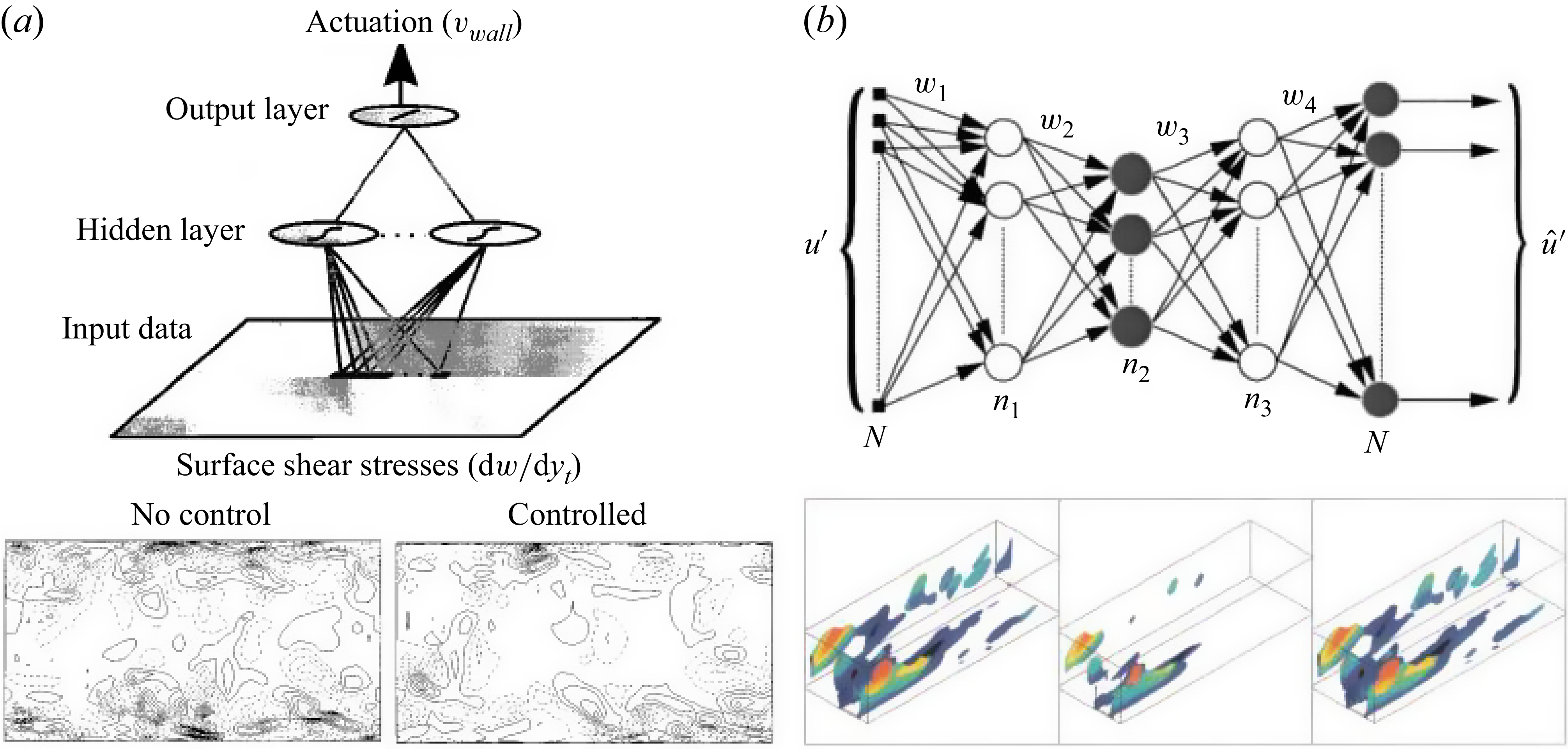
 (a)
 (b)
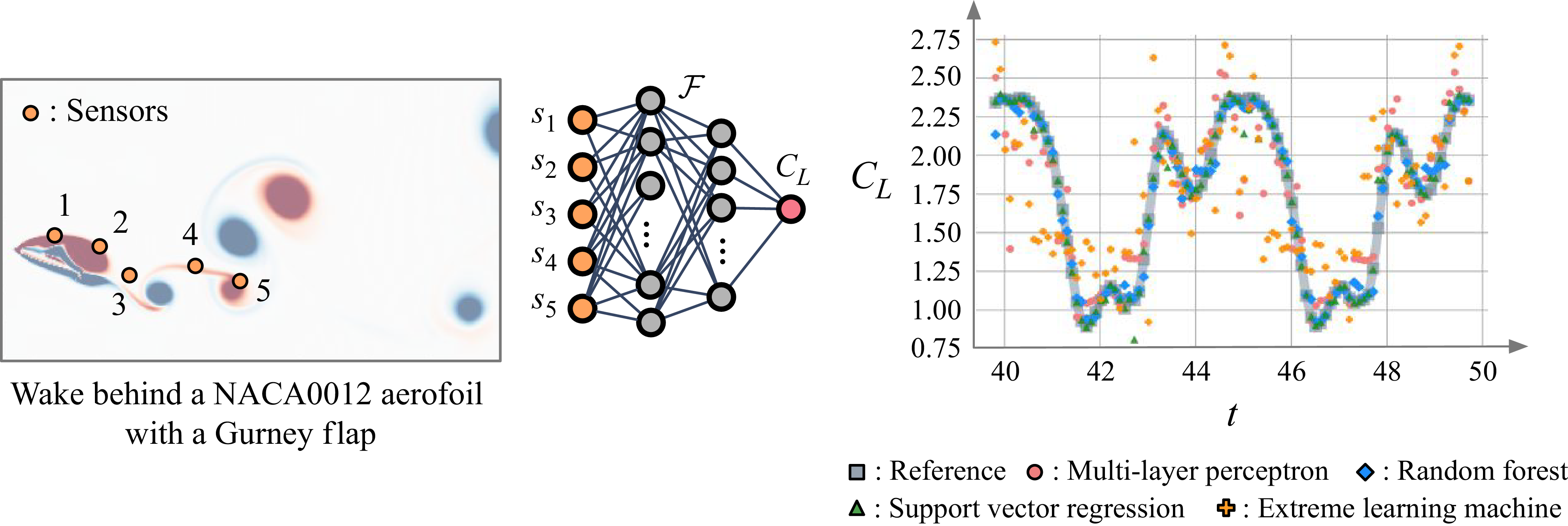
 CL
 Rec=1000
 F:s(t)→CL(t)
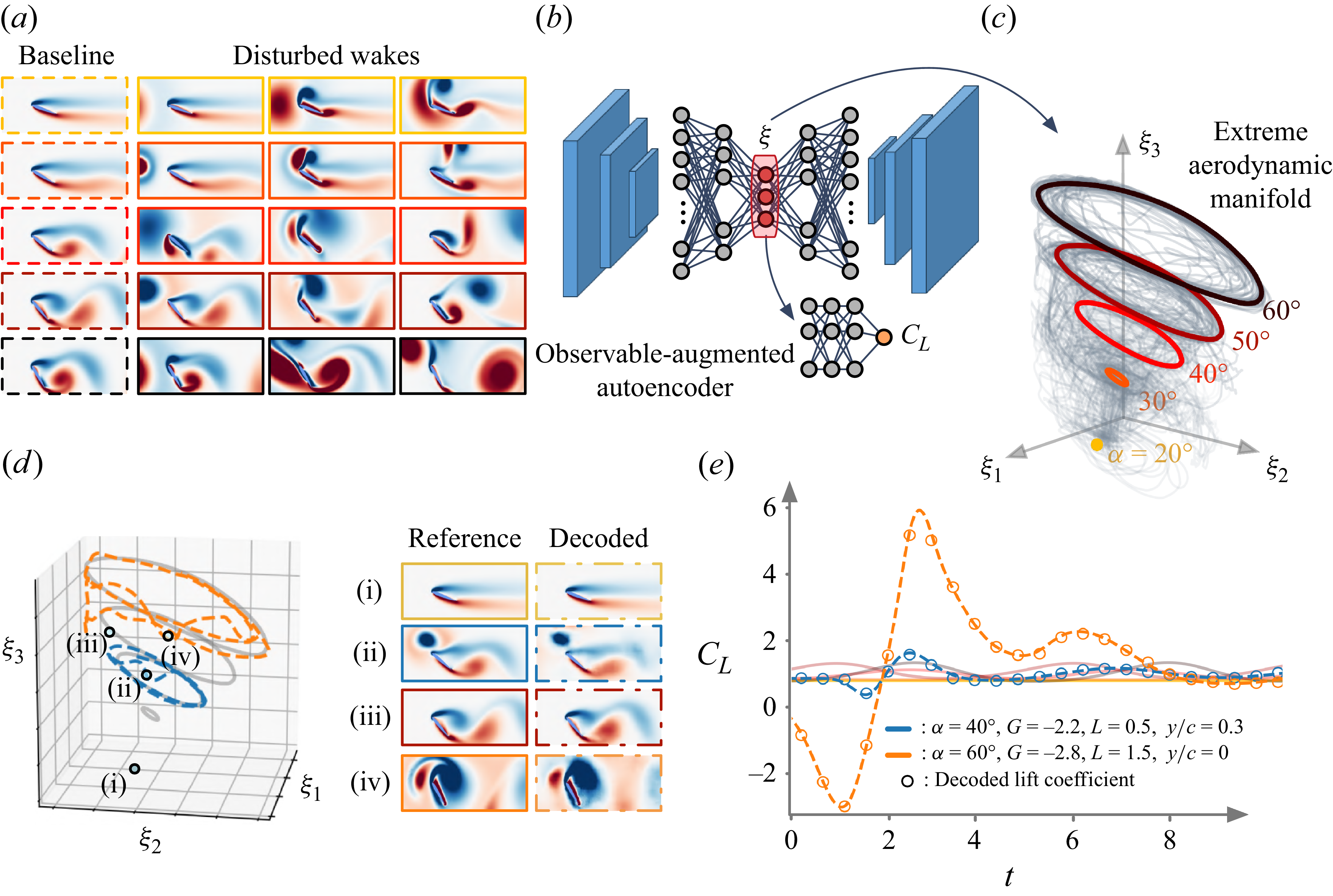
 (a)
 (b)
 (c)
 ξ
 (d)
 (e)
 CL
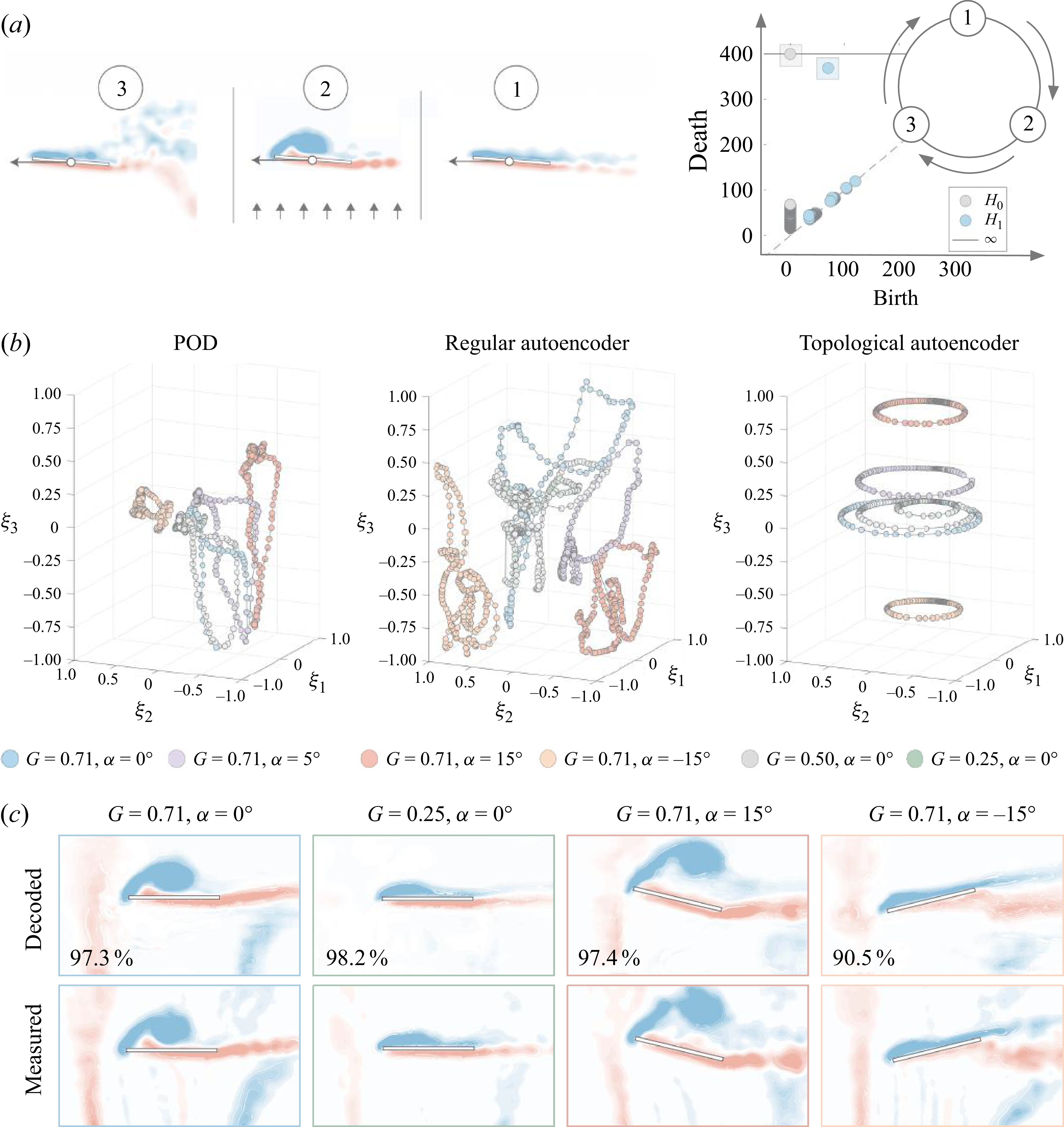
 (a)
 (b)
 (c)

 (a)
 (b)
 L2

 (c)
 Q
 (d)
 x−z

 (a)
 (b)

 (a)
 (b)
 (c)

 (a)
 (b−d)
 (b)
 D
 a
 (c)
 (d)


 qin
 qout

 (a)
 (nsensor×nt)
 (b)
 ngrid×nt
 (c)
 nt×nx×ny×nz×nvariable

 (a)
 (b)
 (c)
 (d)
 (e)
 (f)


 (a)
 (b)

 L2

 (a)
 εd
 ||w||
 (b)
 εd
 εp,1
 (c)
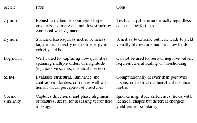

 L2

 (a)
 (b)
 (c)

 Rec=5000
 (a)
 nξ=3
 (b)
 (c)
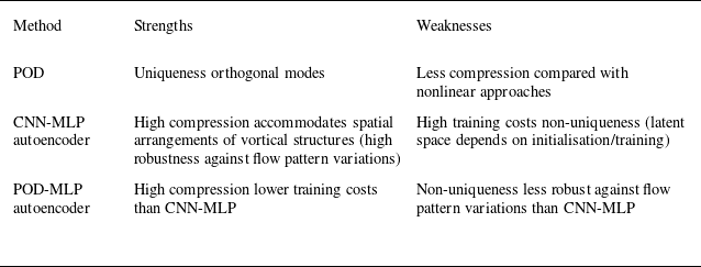

 Rec
 L2
 ε
 Q
 ωz

 (a)
 nw
 (b)
 nw

 nξ=3

 Q

 (a)
 Fs
 Fd
 ns=6
 (b)
 (a)
 L2

 nsnapshot
 ns=12
 L2
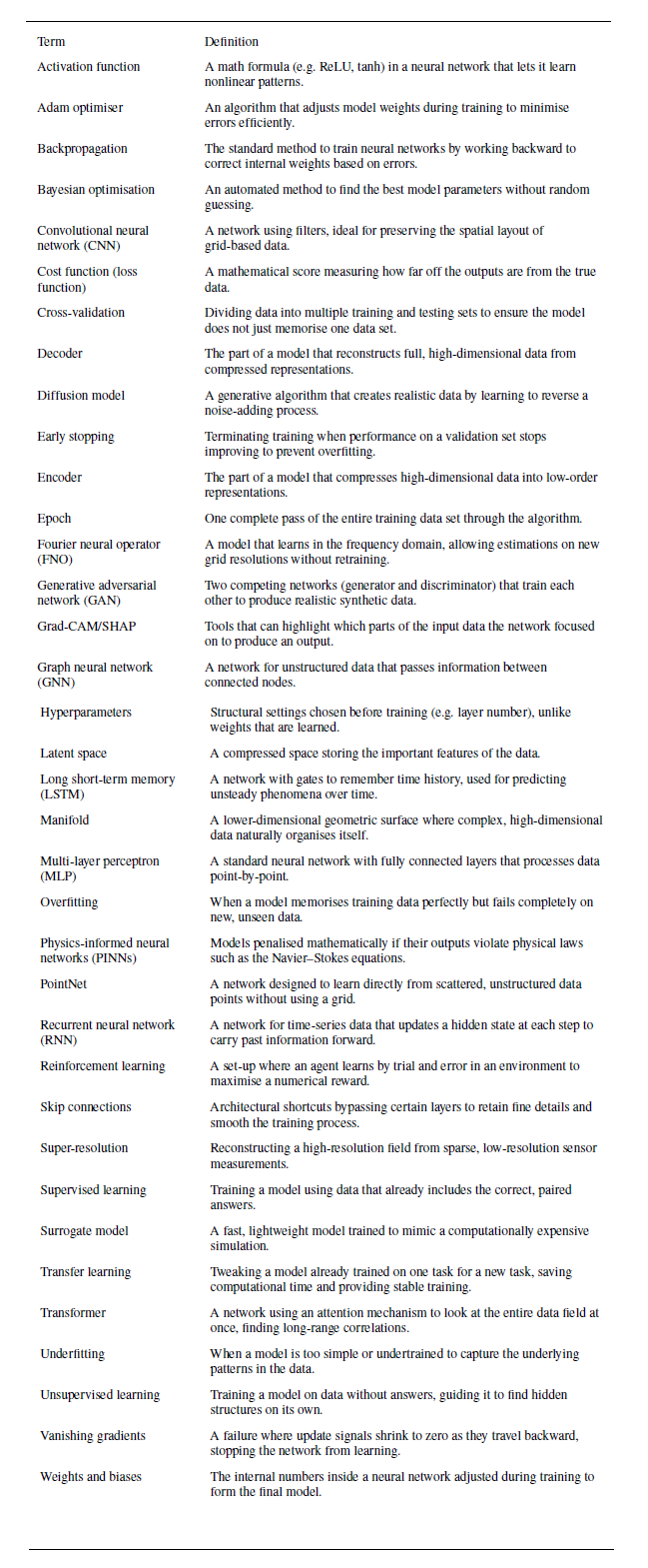

 Open access

