


Impact Statement
Plastic waste is a growing global challenge that affects the environment, resource availability, and long-term sustainability. Progress toward circular materials systems depends on the ability to predict how plastics change during use, recycling, and reprocessing, because poor predictive capability limits the design of efficient recovery strategies. Computational modeling offers a cost-effective and scalable way to examine polymer transformations that remain difficult to isolate experimentally across multiple length and time scales. Our work introduces a predictive and reproducible multiscale simulation framework for systematically analyzing polymer transformations and linking molecular-scale changes to material behavior. A step-by-step tutorial, together with practical guidelines and tools, shows how researchers can apply the framework and adopt it more readily across research and engineering settings. Greater reliability, consistency, and accessibility in polymer transformation modeling can support better decisions in recycling and remanufacturing. Broader use of such predictive tools can help reduce waste, extend material lifetimes, improve resource efficiency, and advance more sustainable production practices.
1. Introduction
Polymers form the backbone of modern technologies in many industries, including biomedical, transportation, food packaging, water treatment, healthcare, and electronics, because of their structural versatility and adjustable chemical functionality [Reference Geyer, Jambeck and Law1, Reference Rudin and Choi2]. Synthetic polymers often go through post-polymerization transformations that tune their structure and composition for specific applications [Reference Ribeiro, Martins, Figueiras, Martins and Gupta3]. Polymer transformation reactions generally fall into two types: functionalization, which modifies chemical groups without breaking the backbone, and depolymerization or degradation, which cleaves covalent bonds to yield smaller fragments [Reference Bultema, Huang, Brauer, Theato, Mazumder, Sheardown and Al-Ahmed4, Reference Clark and Shaver5, Reference García6]. Common transformations include backbone scission, elimination, substitution, isomerization, addition, melting, and crosslinking [Reference Ceretti, Edeleva, Cardon and D’hooge7], which together enable material recovery either as initial monomers and oligomers or as new materials with tailored properties [Reference Ribeiro, Martins, Figueiras, Martins and Gupta3, Reference Hopewell, Dvorak and Kosior8, Reference Hamad, Kaseem and Deri9, Reference Rahimi and García10, Reference Martín, Mondelli, Jaydev and Pérez-Ramírez11, Reference Li, Aguirre-Villegas and Allen12]. Understanding how these transformations proceed along the polymer chain is crucial for designing sustainable materials, circular manufacturing strategies, and efficient recycling and upcycling platforms.
Computational modeling provides a powerful route to study polymer transformations from atomic to mesoscopic scales and complements experiment by helping interpret observations and optimize reaction conditions [Reference Hu13, Reference Gronau, Krishnaji and Kinahan14, Reference Deglmann, Schäfer and Lennartz15, Reference Schmid16]. Common computational approaches for polymer transformations include molecular dynamics (MD; classical and reactive force fields such as ReaxFF), quantum chemical methods (density functional theory (DFT), semi-empirical methods (SEMs), ab initio molecular dynamics (AIMD), and coupled-cluster (CC) theory), kinetic modeling (mechanistic ordinary differential equation models, microkinetic models (MKMs), and kinetic Monte Carlo (kMC)), and machine learning (ML)–based models [Reference Gooneie, Schuschnigg and Holzer17, Reference Gartner and Jayaraman18, Reference Keith, Vassilev-Galindo and Cheng19, Reference Andraju, Curtzwiler, Ji, Kozliak and Ranganathan20, Reference Cao, Zhang, Sun, Yin and Feng21].
Classical MD captures polymer motion, chain packing, and solvent interactions over long length and time scales, but cannot describe chemical transformations. ReaxFF overcomes this limitation by allowing bond breaking and formation, but it relies on large, chemistry-specific parameter sets fit to quantum and experimental data, and their optimization and transferability remain challenging [Reference van Duin, Dasgupta, Lorant and Goddard22, Reference Senftle, Hong and Islam23, Reference Stoliarov, Westmoreland, Nyden and Forney24, Reference Lu, Wang and Li25, Reference Guo, Fan, Guo and Wang26, Reference He and Chen27, Reference Panczyk and Nieszporek28, Reference Ma, Zou and Chen29, Reference Xuan, Cao, Dong and Xia30, Reference Panczyk, Nieszporek and Wolski31, Reference Wolf and Vallverdu32, Reference Xuan, Gao and Ma33, Reference Feng, Zhen and Xu34, Reference Lazarenko, Schmidt, Crowley, Beckham and Knott35]. Quantum chemical methods provide more accurate energetics than ReaxFF, with DFT as the most cost-effective choice. DFT studies report thermodynamic and kinetic parameters, identify competing reaction pathways, and characterize electronic structure and spectroscopic signatures that compare directly with experiment [Reference Lazarenko, Schmidt, Crowley, Beckham and Knott35, Reference Meier and Kip36, Reference Wang, Wang, Liu and Peng37, Reference Shigemoto, Kawakami, Taiko and Okumura38, Reference Huang, Li and Zeng39, Reference Ju40, Reference Bertin, Leblanc, Marque and Siri41, Reference Ghosh, Makeev and Qi42, Reference Huang, Li and Meng43, Reference Jiang, Li and Cui44, Reference Huang, Meng and Luo45, Reference Kolganov, Sreenithya and Pidko46, Reference Pan, Wang and Jin47, Reference Liu, Zhang and Gu48, Reference Papanikolaou, Wu, Huber and Mavrikakis49, Reference Gong, Pan, Cui and Zhang50, Reference Fernández, Palomo and Ortega-Toro51, Reference Luo and Li52, Reference Zhang, Yao and Wang53]. Relative to classical molecular dynamics and reactive force-field methods, DFT requires substantially greater computational effort and therefore restricts polymer models to short oligomers or molecular fragments. Short-fragment models can nevertheless provide reliable activation barriers when the selected structure preserves the local steric, electronic, and conformational environment that affects the reaction step. To bridge from oligomer-scale mechanisms to macroscopic behavior, researchers build kinetic models informed by experimental or quantum-derived rate constants, which predict chain-length distributions, product yields, and catalyst performance over experimentally relevant time scales [Reference Locaspi, Pelucchi and Faravelli54, Reference Guironnet and Peters55, Reference Ejiogu and Peters56, Reference Kruse, Woo, Wong, Khan and Broadbelt57, Reference Bose and Git58, Reference Chen, Ejiogu and Peters59, Reference Chen, Sadow and Peters60, Reference Yappert and Peters61, Reference Dogu, Conka and Akin62, Reference Wang, Wang, Luo and Zhou63, Reference Alqarni64, Reference Palmay, Pillajo, Andrade, Medina and Barzallo65, Reference Wang and Broadbelt66, ,Reference Viet, Weihs, Rajarathnam and Abbas67, Reference Woo and Broadbelt68, Reference Harmon, SriBala, Broadbelt and Burnham69, Reference Kruse, Woo and Broadbelt70, Reference Broadbelt, Stark and Klein71, Reference Woo, Kruse and Broadbelt72, Reference Kruse, Levine and Wong73]. Within this family, kMC propagates individual reaction events without mean-field assumptions, capturing spatial correlations and rare events that analytical and microkinetic models miss and extending accessible polymer lengths and times beyond those reachable by classical MD [Reference Voter, Sickafus, Kotomin and Uberuaga74]. More recently, ML models for polymer degradation and depolymerization use quantum-chemical and experimental descriptors to learn structure–reactivity and structure–property relationships and to screen polymer chemistries more efficiently by reducing the number of costly high-level (HL) quantum chemical calculations required [Reference Keith, Vassilev-Galindo and Cheng19, Reference Cao, Zhang, Sun, Yin and Feng21, Reference Yuan, Hibi and Tamura75, Reference Atasi, Kern and Ramprasad76, Reference Huo, Xie and Tong77, Reference Hu, Sparrow and Ernst78].
Multiscale computational strategies now bridge microscopic chemistry and macroscopic behavior, allowing simulations to interpret properties and guide polymer design beyond synthesis. Existing workflows combine DFT or Quantum Mechanics/Molecular Mechanics (QM/MM) with MD or ReaxFF, kMC or microkinetic models, and in some cases, reactor descriptions to link elementary energetics and atomistic dynamics to degradation, aging, and recycling behavior [Reference Gooneie, Schuschnigg and Holzer17, Reference Bealing and Ramprasad79, Reference Fermeglia and Pricl80, Reference Xie, Wittreich and Vlachos81, Reference Xuan, Wang, Yan and Xia82, Reference Wei, Li, Wang and He83, Reference Meng, Jin and Yang84, Reference Ntioudis, Ewen, Dini and Turner85, Reference Santos, da Costa, Silva, Skaf and Lameira86, Reference Olowookere and Turner87, Reference Mieda88, Reference Trigilio, Marien, Van Steenberge and D’hooge89]. Prior analyses have not fully integrated conformer-resolved polymer models, benchmarked quantum chemical energetics, and graph-based lattice kMC into a single workflow that propagates local reaction events along explicit polymer-chain environments without empirically fitted kinetic parameters. Recent advances in conformer analysis and in HL ab initio methods [Reference Bannwarth, Ehlert and Grimme90, Reference Grimme91, Reference Pracht, Bohle and Grimme92, Reference Riplinger, Sandhoefer, Hansen and Neese93, Reference Rolik, Szegedy, Ladjánszki, Ladóczki and Kállay94, Reference Riplinger and Neese95, Reference Liakos, Sparta, Kesharwani, Martin and Neese96, Reference Riplinger, Pinski, Becker, Valeev and Neese97], particularly local CC approaches that afford near-chemical-accuracy energetics at tractable cost [Reference Liakos, Sparta, Kesharwani, Martin and Neese96], now make rigorous, accurate quantum-chemical kinetic-models feasible. The MUltiscale SImulation frameworK (MUSIK) builds on these developments by combining MD or SEM-informed conformational analysis, DFT geometry optimizations, CC-level ab initio energetics, and lattice-based kMC to model polymer transformations without empirically fitted parameters to resolve spatial kinetics in plastic transformations [Reference Ezendu, Soyemi and Szilvási98, Reference Ezendu and Szilvási99]. We emphasize that previous MUSIK applications to polyvinyl chloride (PVC) dehydrochlorination and depolymerization via olefin metathesis reproduced experimental conversion or yield and structural-evolution trends without parameter fitting.
In this study, we provide a detailed tutorial of MUSIK for polymer transformations. Our goal is to provide all details, including how to set up, run, and interpret results in MUSIK [Reference Ezendu, Soyemi and Szilvási98, Reference Ezendu and Szilvási99]. We illustrate the complete workflow using the previously studied degradation of PVC via base-assisted dehydrochlorination as a case study [18]. The tutorial moves from computational methods and inputs through construction of a kMC model under experimentally relevant conditions, to post-processing of trajectories into rate, mechanistic, and structural outputs. Although this tutorial focuses on elimination, addition, and substitution of functional groups along polymer chains, the same workflow extends to other transformations, including depolymerization and degradation chemistries. We aim for this work to help advance mechanistically informed modeling strategies for polymer upcycling, which can eventually support efforts in plastic circularity, including recycling, upcycling, and sustainable materials design. First-time users may focus on the core workflow steps in Sections 2.1–2.5 and the associated Good Practices and Recommendations, which provide the essential steps for constructing and analyzing a MUSIK model. Advanced users who plan to adapt MUSIK to new polymer chemistries can use the detailed discussions of DFT method selection, solvation treatment, and HL benchmarking in Sections 2.1.2–2.1.4 to validate system-specific energetics.
2. Methods
In this section, we introduce our MUSIK framework, a computational workflow that integrates quantum chemical calculations (e.g., DFT and local coupled cluster methods) with lattice-based kMC to study polymer transformations [Reference Ezendu, Soyemi and Szilvási98, Reference Ezendu and Szilvási99]. We present an overview of the MUSIK workflow in Figure 1. This section is organized according to each stage of the workflow as follows: Section 2.1 describes recommended practices for choosing a computational method and model that best represent the local chemical environment of the polymer. The generation and selection of low-energy conformers that define the polymer geometry are discussed in Section 2.2. Section 2.3 covers the construction of the reaction mechanism, including how to calculate pre-exponential factors and activation energies that serve as inputs for the kMC simulation. We describe the setup and execution of the kMC simulation in Section 2.4. Lastly, different ways of interpreting the output of the kMC simulation are presented in Section 2.5, including how to extract kinetic trends and structural insights from the evolving model.
MUltiscale SImulation frameworK (MUSIK). The workflow links method and model selection, conformer analysis, reaction-mechanism calculation, and activation-energy calculation to lattice-based kinetic Monte Carlo simulations. Result analysis extracts kinetic and structural outputs from kMC trajectories, while the dashed feedback arrow indicates iterative refinement of model assumptions and computational inputs.

2.1. Model and Method Selection
Accurate simulation of polymer transformations begins with selecting a structural model that reproduces the steric and electronic environment of the polymer backbone while remaining computationally tractable. After defining such a model, the next step is to identify quantum chemical methods that provide reliable reaction energetics by benchmarking candidate combinations of density functional, basis set, and solvation model against a local CC reference. Once the computational method is in place, the focus shifts to validating the structural model by varying the polymer chain length and confirming that the key reaction energetics converge. We highlight good practices and target recommendations throughout model selection, method benchmarking, solvation treatment, and model validation. Evidence from prior studies shows that careful selection and testing of both the polymer model and the computational method yield reliable simulations of polymer transformations [Reference Ezendu, Soyemi and Szilvási98, Reference Ezendu and Szilvási99].
2.1.1. Polymer Model Selection
Constructing representative polymer fragments is a critical step in modeling polymer transformations, since model size effects, steric hindrance, and electronic delocalization strongly influence calculated energetics. We recommend short polymer fragments that reproduce the local electronic and steric environment of the reaction center while keeping the calculations computationally efficient [Reference Papanikolaou, Wu, Huber and Mavrikakis49, Reference Ezendu, Soyemi and Szilvási98, Reference Ezendu and Szilvási99, Reference Wu, Papanikolaou and Cheng100]. Each new polymer system nevertheless requires fragment-size validation because chain-length effects, stereochemistry, and conformational constraints can alter the reaction energetics. Researchers can perform that validation by increasing fragment length until activation barriers and reaction energies no longer change significantly. To avoid artifacts from chain ends, we embed the reacting monomer unit within the fragment and include enough neighboring monomer units to capture inductive and conjugative interactions that significantly influence local reactivity.
Polymer fragments can adopt multiple conformations and distinct stereochemical configurations, such as cis (Z) or trans (E) isomers and isotactic or syndiotactic chain arrangement. When experimental or computational precedent exists, literature reports can guide the choice of conformation or isomer. In the absence of such guidance, researchers can compare activation barriers across candidate isomers for a key reaction step and select the configuration with the lowest energy pathway while considering reaction center location. End-chain and mid-chain environments impose different steric and backbone constraints and therefore alter the accessible conformational space. To avoid chain-end artifacts, we embed the reacting monomer unit within the fragment and include enough neighboring monomer units to capture inductive and conjugative interactions that significantly influence local reactivity [Reference Ezendu, Soyemi and Szilvási98, Reference Ezendu and Szilvási99]. Researchers can address the reduced flexibility imposed by mid-chain environments by introducing strain through incremental increases in the distance between the terminal carbon atoms of the fragment and then evaluating the resulting changes in Gibbs energies and activation barriers [Reference Lugo, Edeleva, Van Steenberge and Sabbe101].
Polymer systems with additional complexity, such as branching, tacticity variations, or chain defects, require additional models that incorporate these features. A common strategy is to modify the repeat/monomer unit at or near the reaction center to represent a structural irregularity, such as replacing a regular monomer with one containing a missing substituent, an added functional group, or an altered stereochemical orientation [Reference Ezendu, Soyemi and Szilvási98]. Embedding the modified monomer within the polymer fragment allows for a direct comparison of reaction energetics and mechanistic pathways between a fragment with a structural defect and its defect-free counterpart. For example, defect-containing fragments have been shown to change the course of reactions along the polymer chain, and such comparisons demonstrate that structural defects can shift activation barriers and modify accessible mechanistic pathways [Reference Ezendu, Soyemi and Szilvási98, Reference Ezendu and Szilvási99].
-
• Use polymer fragments that balance chemical realism with computational efficiency; 3–5 monomer units are often sufficient.
-
• Place the reacting monomer away from chain termini and use appropriate capping groups to prevent artificial polarization.
-
• Preserve inductive and conjugative influences from adjacent units when defining chain ends to preserve local electronic effects.
-
• Evaluate relevant conformers or stereoisomers; compare activation barriers if no precedent study exists.
-
• Incorporate branching, tacticity, or structural defects into additional models when these features may influence reactivity.
Good Practices and Recommendations
2.1.2. Choice of DFT Method
Selecting an exchange–correlation functional is a nontrivial choice in DFT studies, since functionals vary in their ability to describe different classes of reactions, and no single option is universally reliable. Hundreds of functionals exist [Reference Mardirossian and Head-Gordon102], organized according to Jacob’s ladder [Reference Perdew and Schmidt103], and it is generally believed that higher rungs offer improved accuracy at higher computational cost [Reference Perdew and Schmidt103]. For polymer transformations that require accurate reaction barriers and reaction energies, the functional must reliably describe bond-breaking and bond-forming events, often in extended, conjugated, or sterically constrained environments. Current computational resources permit geometry optimizations with functionals at rung 3 or higher for polymer fragments, including meta-generalized gradient approximation (GGA) and hybrid DFT functionals [Reference Mardirossian and Head-Gordon102]. Functionals such as PBE0 [Reference Perdew, Burke and Ernzerhof104, Reference Adamo and Barone105], B3LYP [Reference Becke106, Reference Chai and Head-Gordon107], M06-2X [Reference Zhao and Truhlar108], and ωB97X-D [Reference Chai and Head-Gordon107, Reference Chai and Head-Gordon109, Reference Zheng, Zhao and Truhlar110] are frequently evaluated, as they have shown consistent performance for barrier calculation relative to HL ab initio methods such as canonical coupled cluster with single, double, and perturbative triple excitations (CCSD(T)) [Reference Riplinger, Sandhoefer, Hansen and Neese93, Reference Bartlett and Musiał111, Reference Raghavachari, Trucks, Pople and Head-Gordon112]. The chemical composition of the full system, including the polymer backbone, substituents, catalyst, and solvent, should guide functional choice because some functionals describe main-group chemistry more reliably, whereas others better capture transition-metal or heavy p-block reactivity. Regardless of the specific choice, most DFT functionals share systematic limitations, particularly self-interaction error (SIE) [Reference Perdew and Zunger113, Reference Mori-Sánchez, Cohen and Yang114, Reference Bao, Gagliardi and Truhlar115, Reference Cohen, Mori-Sánchez and Yang116] and the inadequate treatment of long-range correlation [Reference Cohen, Mori-Sánchez and Yang116]. Self-interaction error arises from the spurious or unphysical interaction of an electron with its own charge density and can strongly affect charged or delocalized states [Reference Perdew and Zunger113, Reference Mori-Sánchez, Cohen and Yang114, Reference Bao, Gagliardi and Truhlar115, Reference Cohen, Mori-Sánchez and Yang116]. Global and range-separated hybrid functionals incorporate a fraction of exact Hartree–Fock exchange, which helps reduce SIE and improves barrier heights and charge localization, particularly for anionic or radical intermediates [Reference Mardirossian and Head-Gordon102, Reference Cohen, Mori-Sánchez and Yang116]. Long-range correlation effects arise from dispersion (London) interactions between distant parts of the polymer or between the polymer and its environment and can significantly alter relative stabilities and barriers [Reference Grimme117, Reference Becke and Johnson118]. Incorporating dispersion corrections is therefore essential because noncovalent interactions can influence both conformational preference and reaction energetics [Reference Chai and Head-Gordon109, Reference Grimme, Antony, Ehrlich and Krieg119]. Dispersion correction methods such as D3 (with zero or BJ damping) [Reference Becke and Johnson118, Reference Grimme, Antony, Ehrlich and Krieg119, Reference Becke and Johnson120], D4 [Reference Caldeweyher, Ehlert and Hansen121], MBD [Reference Tkatchenko, DiStasio, Car and Scheffler122, Reference Tkatchenko and Scheffler123], VV10 [Reference Vydrov and Van Voorhis124, Reference Liang, Feng, Hait and Head-Gordon125], or XDM [Reference Becke and Johnson120, Reference Johnson and Becke126, Reference Johnson and Becke127] can be added to most functionals [Reference Grimme, Hansen, Brandenburg and Bannwarth128], while others, such as ωB97X-D, include dispersion treatment intrinsically. We recommend applying dispersion corrections consistently across reactants, intermediates, and transition states so that their relative energies remain comparable and are not biased by inconsistent dispersion treatment.
Once a suitable functional has been chosen, the next step is to select a basis set that can describe bond breaking and formation along the reaction coordinate and yield reliable reaction and activation energies. A well-chosen basis set includes polarization functions to describe bond breaking and formation, diffuse functions to treat anions and other loosely bound electrons, and sufficient valence functions to capture electron correlation accurately. Increasing the size and completeness of a basis set generally improves the description of the electron density but also increases computational cost. Minimal and small split-valence basis sets lack sufficient functions per atom to reliably describe bond rearrangements, which increase basis set incompleteness error (BSIE) and basis set superposition error (BSSE) [Reference Helgaker, Jorgensen and Olsen129, Reference Bursch, Mewes, Hansen and Grimme130]. Basis set incompleteness error occurs when the basis set is too small to accurately describe the electronic structure of the polymer fragment, while BSSE arises from overlapping basis functions between interacting fragments because the basis set is too small [Reference Helgaker, Jorgensen and Olsen129, Reference Bursch, Mewes, Hansen and Grimme130, Reference Van Mourik, Wilson, Peterson, Woon, Dunning and Sabin131, Reference Balabin132]. Both errors can distort bond lengths, angles, and dihedrals, shift reaction and barrier energies, and artificially stabilize polymer intermediates and transition states [Reference Van Mourik, Wilson, Peterson, Woon, Dunning and Sabin131, Reference Balabin132]. To minimize these errors, larger basis sets such as quadruple-ζ(Z) can significantly decrease basis set errors but may be impractical for routine geometry optimizations. In practice, a cost-effective polarized basis set can be used for geometry optimizations, with larger basis sets such as triple- or quadruple-ζ(Z) applied for single-point energy calculations when resources permit. Common Gaussian-type basis sets include those from the Pople [Reference Ditchfield, Hehre and Pople133, Reference Hehre, Ditchfield and Pople134], Dunning [Reference Dunning135, Reference Wilson, van Mourik and Dunning136], Ahlrichs [Reference Weigend, Häser, Patzelt and Ahlrichs137, Reference Weigend and Ahlrichs138], and Jensen [Reference Jensen139, Reference Jensen140] families, each providing a systematic hierarchy that increases the level of theory and calculation accuracy [Reference Dunning135, Reference Jensen141]. We recommend the Ahlrichs basis set family, as they are consistently available for most elements on the periodic table. We find that diffuse functions are generally unnecessary for neutral covalent polymers but are important for systems with significant negative charge density or for polarizability calculations. For heavy atoms beyond the fourth period, one should combine scalar-relativistic Hamiltonians (such as DKH [Reference Reiher142], ZORA [Reference Pollak and Weigend143, Reference Centoducatte, de Oliveira, Jorge and Camiletti144], or X2C [Reference Kutzelnigg and Liu145, Reference Saue146]) with compatible scalar-relativistic basis sets (for example, SARC [Reference Pantazis, Chen, Landis and Neese147], ANO [Reference Almlöf and Taylor148, Reference Widmark, Zobel, Vysotskiy, Tsuchiya and Veryazov149], or def2 variants [Reference Pollak and Weigend143]) to capture relativistic effects that can significantly influence bond lengths, bond strengths, and reactivity.
-
• Survey commonly used functionals for the reaction type of interest and then evaluate their accuracy through benchmarking (see Section 2.1.4).
-
• Include dispersion correction in all calculations.
-
• Evaluate basis sets on the chosen polymer fragment by checking convergence of geometry and reaction energetics to ensure the basis set is large enough to capture bond-breaking and bond-formation while remaining computationally efficient.
-
• Always use diffuse functions when modeling anions, highly polar transition states, or polarizability.
-
• Apply effective core potentials or scalar-relativistic corrections for heavy atoms (N > 36).
Good Practices and Recommendations
2.1.3. Solvation Model
Solvent effects significantly influence the energetics of polymer transformations since changes in polarity, dielectric constant, or hydrogen-bonding environment can stabilize or destabilize reactants, intermediates, and transition states. Neglecting solvation can thus lead to substantial errors in calculated barriers and reaction energies, and sometimes result in qualitatively incorrect electronic structures. In practice, the solvent can be treated with continuum (implicit) models, microsolvation clusters, or fully explicit solvent molecules, depending on the level of detail and computational cost one is willing to accept [Reference Harvey, Himo, Maseras and Perrin150, Reference Tomasi151]. Explicit solvation is computationally demanding for polymer transformations because it requires sampling polymer fragments with many explicit solvent molecules. Therefore, the MUSIK framework uses implicit solvation models as the standard approach, balancing accuracy and efficiency. Implicit or continuum models like SMD [Reference Aleksandr, Marenich and Truhlar152], CPCM [Reference Barone and Cossi153, Reference Takano and Houk154], or COSMO-RS [Reference Klamt155, Reference Klamt and Schüürmann156] capture bulk dielectric properties and non-electrostatic effects, providing an efficient way to include solvent effects. However, because implicit solvation models average the solvent response, they may underestimate activation barriers in systems where strong localized solute–solvent interactions are important [Reference Harvey, Himo, Maseras and Perrin150, Reference Ryu, Park and Kim157]. The effect is even more pronounced when dispersion corrections are neglected [Reference Chai and Head-Gordon109, Reference Edeleva, Van Steenberge, Sabbe and D’hooge158]. While continuum models work well for many polymers with nonpolar backbones [Reference Ezendu, Soyemi and Szilvási98, Reference Ezendu and Szilvási99], systems with polar functional groups, hydrogen-bonding motifs, or intermediates with partial charge separation can be more sensitive to solvation. In such cases, implicit models generally predict the correct qualitative trends, but further benchmarking against higher-level calculations or explicit-solvent cluster models may be necessary for precise reaction energetics.
-
• Choose the solvation model and solvent parameters to reflect the experimental medium or the intended reaction environment.
-
• Apply the solvation model consistently across reactants, intermediates, and transition states to avoid systematic shifts in relative energetics.
Good Practices and Recommendations
2.1.4. Benchmarking and Selecting Computational Methods
Benchmarking establishes the reliability of candidate DFT methods by comparing their calculated energetics with a HL reference. The goal is to identify a functional–basis set combination that reproduces barrier heights and reaction energies with sufficient accuracy for polymer transformations, while remaining computationally tractable.
Selecting an appropriate reference method is essential for reliable benchmarking [Reference Mata and Suhm159]. Canonical CCSD(T) [Reference Riplinger, Sandhoefer, Hansen and Neese93, Reference Raghavachari, Trucks, Pople and Head-Gordon112] serves as the gold standard for small molecules, but it is prohibitively expensive for larger systems because of its computational cost [Reference Liakos, Sparta, Kesharwani, Martin and Neese96, Reference Bartlett and Musiał111]. Local CC methods such as DLPNO–CCSD(T) [Reference Riplinger and Neese95, Reference Riplinger, Pinski, Becker, Valeev and Neese97] or LNO-CCSD(T) [Reference Rolik, Szegedy, Ladjánszki, Ladóczki and Kállay94, Reference Nagy, Samu and Kállay160] provide a practical alternative, offering accuracy close to canonical CCSD(T) while reducing the formal scaling to nearly linear with system size. High-level CC approaches, both canonical and local variants, are implemented in widely used software packages such as ORCA [Reference Neese161, Reference Neese162], MRCC [Reference Kállay, Nagy and Mester163, Reference Mester, Nagy and Csóka164], and MOLPRO [Reference Werner, Knowles, Knizia, Manby and Schütz165, Reference Werner, Knowles and Manby166], with more recent interfaces also available in PySCF [Reference Sun, Berkelbach and Blunt167, Reference Sun, Zhang and Banerjee168].
We suggest benchmarking as follows: First, we optimize the geometries of representative polymer fragments with candidate DFT functionals in widely available software such as Gaussian [Reference Frisch, Trucks and Schlegel169], ORCA, Q-Chem [Reference Kong, White and Krylov170, Reference Shao, Gan and Epifanovsky171], or NWChem [Reference Mejia-Rodriguez, Aprà and Autschbach172, Reference Valiev, Bylaska and Govind173]. Next, we compute single-point reference energies at the HL using these DFT-optimized geometries and compare reaction energies and barrier heights using DFT against the HL reference values using error metrics such as mean absolute error, root-mean-square error, or maximum deviation. Then, we select the DFT method that gives reaction and barrier energies in closest agreement with the HL reference across all benchmarked steps. In parallel, we also benchmark the structure of representative intermediate(s) or transition state(s) across the tested DFT functionals and basis sets. We recommend comparing key reaction coordinate bond lengths, angles, or dihedrals across the tested DFT methods; if these metrics do not change significantly, the chosen basis set is adequate for HL single-point calculations. Accurate geometries are essential because differences in bond lengths, angles, or torsions lead directly to errors in the HL energies, reducing the reliability of the benchmark. It should be noted that basis-set errors, including BSIE and BSSE (see Section 2.1.2), reduce accuracy at every stage of benchmarking, from geometry optimization and transition-state searches up to HL single-point energy calculations. Therefore, to minimize these errors, use at least triple-ζ basis sets for single-point energy calculations, include diffuse functions for weakly bound regions, and check basis-set convergence for systems with multiple interacting fragments. For consistency, apply the same solvation model and dispersion correction to all species and calculations to maintain comparability and prevent systematic errors in relative energies.
Once a suitable computational method is established, we recommend reiterating the model benchmark and validating the fragment size separately to confirm that the model captures the steric and electronic influences of the polymer environment. One can perform model validation by calculating reaction energetics, either electronic energies or Gibbs free energies, for progressively longer chain fragments until the values converge. Convergence demonstrates that the selected computational setup is likely transferable across system sizes.
-
• Benchmark DFT methods systematically by varying the type of functionals, basis sets, dispersion corrections, and solvation models to identify combinations that yield reliable energetics.
-
• Keep geometries and solvation models consistent between DFT and HL reference calculations so that differences arise only from the electronic structure method.
-
• Use local CC methods as the HL reference method.
-
• For more accurate reference energies, apply at least triple-ζ basis sets to minimize BSIE and BSSE.
-
• Reiterate model and method benchmarking to validate that the model and method consistently produce accurate results
Good Practices and Recommendations
2.2. Conformer Analysis
Identifying the most relevant conformational states of a polymer fragment is essential for obtaining meaningful reaction energetics. Structural flexibility arising from backbone rotations, side-chain motions, or branching can significantly alter activation barriers and thermodynamic stability. Even fragments that appear rigid may have several low-lying conformers within a narrow energy range, making conformer analysis a critical step in modeling polymer transformation. Because full DFT conformational sampling is often expensive for large fragments, we adopt a multi-level approach: conformers are first generated at a lower level of theory and then refined at the chosen DFT level.
Practitioners commonly generate conformers using semiempirical or tight-binding quantum methods, which balance speed and accuracy and have been benchmarked extensively on organic backbones. The MUSIK framework relies on methods from the GFNn − xTB (n = 1 or 2) [Reference Bannwarth, Ehlert and Grimme90, Reference Grimme91] family for routine conformer sampling, which provide reliable starting points for diverse systems. Conformer searches aim to map torsional rotations, ring puckering, and side-chain motions, which together define the accessible conformational space. Search algorithms typically generate a large number of candidate geometries, either by systematic torsion driving, stochastic sampling, or enhanced sampling techniques such as metadynamics. Post-processing reduces the raw ensemble by pruning duplicates, re-ranking structures by relative energy, and retaining only distinct low-energy candidates for further calculations. Computational workflows commonly use software packages such as CREST [Reference Pracht, Bohle and Grimme92], CENSO [Reference Grimme, Bohle and Hansen174], RDKit [Reference Bento, Hersey and Félix175], OMEGA [Reference Hawkins, Skillman, Warren, Ellingson and Stahl176], and ConfGen [Reference Watts, Dalal and Murphy177] to generate conformers, prune ensembles, and prepare inputs for subsequent DFT optimization. Recent developments have introduced ML-based approaches for conformer generation, in which data-driven models learn molecular energetics and conformational preferences from reference DFT datasets to guide efficient exploration of low-energy regions at near-DFT accuracy [Reference Wood178, Reference Jiang, Gogineni and Kammeraad179, Reference Guo, Fang and Xu180, Reference Gogineni181, Reference Tayfuroglu, Zengin, Koca and Kocak182, Reference Taneja and Lasker183, Reference Grambow, Weir, Cunningham, Biancalani and Chuang184]. Although ML-based methods are not employed here, they represent a complementary and rapidly advancing direction that might be relevant for MUSIK in the very near future.
Following the generation of conformers, select low-energy candidates from the conformer ensemble within 20–25 kJ mol−1 of the global minimum. Reoptimize each candidate at the chosen DFT level to refine the electronic structure and remove semiempirical stage artifacts. The DFT global minimum generally serves as the representative geometry for reaction energy and barrier calculations, with higher-energy conformers included via Boltzmann distribution only if they significantly contribute to the reaction temperature.
-
• Always perform conformer analysis and ensure that low-energy candidates are structurally unique.
-
• Use efficient semiempirical, tight-binding, or ML interatomic potential-based methods for initial conformer sampling to balance accuracy and cost.
-
• Record and archive all search parameters, conformer geometries, and results to ensure reproducibility.
Good Practices and Recommendations
2.3. Reaction Mechanism Calculation
Developing a reaction network begins with identifying all chemically plausible elementary transformation steps consistent with the intended reaction chemistry. Insights from literature, including both computational and experimental studies, can guide the selection of elementary steps. For each elementary step, one must optimize the corresponding intermediates and transition states at the selected DFT level and confirm them through vibrational frequency analysis. It is a must to identify local minima by the absence of imaginary frequency and transition states by a single imaginary frequency along the reaction coordinate. We also recommend performing intrinsic reaction coordinate (IRC) analysis to confirm that each transition state connects to the expected minima [Reference Fukui185, Reference Maeda, Harabuchi, Ono, Taketsugu and Morokuma186]. To ensure that calculations use thermodynamically relevant structures, apply the conformer analysis described in Section 2.2 to each reactant, intermediate, transition state, and product state. Use the lowest-energy DFT-optimized conformers as input geometries for calculating reaction energies and barrier heights with the chosen HL electronic structure method. Obtain reaction energies and barrier heights in three stages, as detailed by the equations in the subsection below:
2.3.1. DFT-Level Energies
At the DFT level, energy barriers are obtained by calculating the electronic energy differences between the transition state or intermediate and the sum of the reactant energies as follows:

where the superscript X refers to either the transition state (‡) or an intermediate or product (INT).
$ {E}_{DFT} $
 represents the total self-consistent electronic energy, typically including dispersion correction.
The Gibbs free energy at the DFT level combines electronic, zero-point, thermal, and entropic contributions:

where
$ {ZPE}_{DFT} $
 is the zero-point vibrational energy,
$ {E}_{Thermal} $
 includes the thermal energy contributions of translational, rotational, and vibrational degrees of freedom, as well as the
$ {k}_BT $
 term, T is the temperature (298 K), and
$ {S}_{DFT} $
 is the entropy term [Reference Frisch, Trucks and Schlegel169, Reference Frisch, Trucks and Schlegel187].
The Gibbs free energy barrier for a step, similar to Equation 1, is calculated as:

Kinetic parameters such as the activation energy and the pre-exponential factor are obtained by substituting the electronic and Gibbs free energies from Equations 1 to 3 into the Arrhenius–Eyring rate constant relationship as shown below:

where A is the pre-exponential factor,
$ {E}_a $
 is the activation energy, R is the universal gas constant, T is the temperature,
$ {k}_BT $
 is the Boltzmann constant, h is Planck’s constant, and
κ
is the transmission coefficient (usually taken as unity). Most studies apply classical transition-state theory (
κ
= 1), which assumes that every trajectory crossing the transition state proceeds directly to products without recrossing and that quantum tunneling through the barrier is negligible. In cases where these assumptions do not hold, a more accurate approach is to include dynamical effects that modify the rate constant through a transmission coefficient that can vary with temperature. We recommend applying methods like canonical variational transition-state theory to capture recrossing and the small-curvature tunneling approximation to describe tunneling, obtaining temperature-dependent transmission coefficients that reveal how these effects alter the overall rate relative to the classical estimate [Reference Truhlar and Garrett188, Reference Bao and Truhlar189, Reference Olajide and Szilvási190]. We recommend that k and A must be checked to ensure that their units remain consistent with the reaction molecularity and the standard-state convention used in Equation 4.
The activation energy at the DFT level is evaluated as:

where
$ {ZPE}_{DFT} $
 is the zero-point vibrational energy,
$ {E}_{Thermal} $
 includes the thermal energy contributions of translational, rotational, and vibrational degrees of freedom as well as the
$ {k}_BT $
 term.
The Arrhenius–Eyring expression in Equation 4 contains both the activation energy and the Gibbs free energy barrier. Substituting the activation energy from Equation 5 and the Gibbs free energy definition from Equation 3 allows the separation of the entropy contribution. The pre-exponential factor is then obtained as:

where Δ
$ {S}_{DFT} $
 is the entropy change between the transition state and the reactants.
2.3.2. Thermochemical Corrections
Accurate modeling in agreement with experiments requires the proper treatment of temperature, pressure, and entropy effects. Neglecting thermodynamic corrections introduces non-systematic errors in free energies, which in turn alter the rate parameters supplied to kMC simulations. In the MUSIK framework, vibrational analyses at the quantum-chemical level provide zero-point energies, thermal contributions, and entropic terms. Post-processing tools such as Shermo [Reference Lu and Chen191], GoodVibes [Reference Luchini, Alegre-Requena, Funes-Ardoiz and Paton192], or Arkane [Reference Dana, Johnson and Allen193] facilitate vibrational analysis and allow the extraction of zero-point, thermal, and entropic contributions directly from DFT calculations. Applying such corrections uniformly across all species ensures that the relative free energy remains comparable to experimental conditions. Free energies are typically referenced to the gas-phase standard state (1 atm) by most quantum-chemical software packages, which should be converted to the 1-M solution standard state when plastic transformations occur in solution. The need for concentration correction becomes critical when the reaction stoichiometry involves a net change in the number of moles, because the standard-state term no longer cancels between reactants and products. The corrected free energy is then:

Here, Δν is the change in the number of moles from reactants to the transition state or intermediate and
$ {c}_{ref}=\frac{p}{RT} $
 is the molar concentration for the gas-phase standard state, where p is the pressure (1 atm), R is the universal gas constant, and T is the reference temperature. For example, a bimolecular association reaction (Δν = −1) at 298 K corresponds to a correction of approximately −1.89 kcal mol−1 or 7.92 kJ mol−1.
2.3.3. High-Level (HL) Single-Point Energies
To achieve near-chemical accuracy in calculated energetics, the MUSIK framework improves upon DFT-level results by applying HL single-point electronic structure methods using local CCSD(T) methods that we find as an affordable balance between accuracy and computational cost. For each reactant, transition state, and intermediate, we calculate HL single-point energies on the DFT-optimized geometry of the lowest-energy conformer.
The activation energy at a higher level of theory is evaluated analogously to the DFT expression in Equation 5:

where
$ \Delta {E}_{HL}^{\ddagger 0} $
 is the CC electronic energy of the transition states. The association/dissociation steps without an internal energy barrier require estimating an effective activation free energy that can be done by applying the translational-entropy penalty for association steps [Reference Ezendu and Szilvási99]. To quantify the translational entropy, we utilize the simplified form of the Sackur–Tetrode equation [Reference Ryu, Park and Kim157, Reference Tetrode194], which separates the contributions of mass and temperature under ideal gas conditions:

where M represents the molar mass, T is the temperature, and R is the ideal gas constant. Consequently, for a 2 → 1 association under the 1-M standard state at 298 K, the translational entropic penalty typically falls in the 40–50 kJ mol−1 range.
The HL Gibbs free energy is obtained by adding DFT-derived thermal corrections to the HL single-point energy:

The final HL Gibbs free energies of intermediates and transition states with correction to the solution-phase standard state are then written as:

We note that forward barriers are evaluated for every elementary step. However, reverse barriers can be calculated and included when their magnitude is small or when the reverse process occurs on a timescale comparable to the forward reaction. A forward barrier corresponds to the Gibbs free energy difference between a transition state and the preceding intermediate or reactant, while a reverse barrier corresponds to the Gibbs free energy difference between the same transition state and the subsequent intermediate or product.
-
• Use near-linear scaling local CCSD(T) methods to obtain accurate HL energies.
-
• Archive all computational data, including optimized DFT geometries, HL single-point calculations, and thermochemical corrections, in accessible repositories to ensure transparency and reproducibility.
Good Practices and Recommendations
2.4. Kinetic Monte Carlo Simulations
Kinetic Monte Carlo simulation is a simulation framework for modeling the time evolution of systems via stochastic steps where transitions between states occur with known rates, typically derived from quantum chemical calculations or experimental measurements [Reference Voter, Sickafus, Kotomin and Uberuaga74, Reference Gillespie195, Reference Stamatakis and Vlachos196, Reference Chatterjee, Vlachos and Katsoulakis197, Reference Collins, Chatterjee and Vlachos198, Reference Gillespie199, Reference Chatterjee and Vlachos200, Reference Lee and Sinno201, Reference Konwar, Bhute and Chatterjee202, Reference Trochet, Mousseau, Béland, Henkelman, Andreoni and Yip203]. The kMC simulation comes in two implementations, on- and off-lattice. On-lattice kMC uses a fixed grid or network of sites and bonds, where each site represents a possible chemical position such as an atom, monomer, or active site. Reactions occur when local arrangements of sites match a predefined pattern, changing the type of a site or the connection between neighboring sites [Reference Voter, Sickafus, Kotomin and Uberuaga74, Reference Gillespie195, Reference Stamatakis and Vlachos196, Reference Chatterjee, Vlachos and Katsoulakis197, Reference Collins, Chatterjee and Vlachos198, Reference Gillespie199, Reference Chatterjee and Vlachos200, Reference Jansen204]. Off-lattice kMC works in continuous 3-D space, where events depend on distances and orientations between moving particles rather than a fixed grid [Reference Konwar, Bhute and Chatterjee202, Reference Trochet, Mousseau, Béland, Henkelman, Andreoni and Yip203], and can be implemented using tree-based or matrix-based formulations for event selection and rate representation [Reference Conka, Akin and Withoeck205, Reference Moens, Marien and Figueira206]. Lattice-based kMC can suit polymer transformations because it preserves chain structure, tracks local environments explicitly, and captures interactions between neighboring units [Reference Viet, Weihs, Rajarathnam and Abbas67, Reference Mätzig, Drache, Drache and Beuermann207, Reference Gao, Oakley, Konstantinov, Arturo and Broadbelt208].
Modeling polymers introduce unique computational challenges because each chain (lattice) contains many reactive sites, and each site can undergo multiple reaction types, yielding thousands of distinct events with rates that depend on local configurations. Event selection and lattice updates become the primary computational bottlenecks, especially when long-range or lateral interactions are included [Reference Pineda and Stamatakis209]. Rejection-free sampling improves computational efficiency by selecting the next event directly from the correct rate distribution, advancing time accordingly, and executing every selected event without unnecessary rejections [Reference Stamatakis and Vlachos196, Reference Collins, Chatterjee and Vlachos198, Reference Chatterjee and Vlachos200, Reference Jansen204, Reference Pineda and Stamatakis209, Reference Andersen, Panosetti and Reuter210]. To make rejection-free sampling efficient, modern implementations organize event data so the algorithm can quickly find the next reaction and update only the local region affected by the last one [Reference Stamatakis and Vlachos196, Reference Pineda and Stamatakis209, Reference Andersen, Panosetti and Reuter210]. In practice, rejection-free sampling often uses graph-based representations [Reference Stamatakis and Vlachos196], where each site or monomer corresponds to a node and a chemical bond or where spatial connections define edges. Events modify only the nodes and edges involved, which allows localized rate updates instead of recalculating the entire system. When applying MUSIK, we recommend using software such as Zacros, kmos [Reference Hoffmann, Matera and Reuter211], KMCLib [Reference Leetmaa and Skorodumova212], MoCKA [Reference Kunz, Kuhn and Deutschmann213], or MonteCoffee [Reference Jørgensen and Grönbeck214] to leverage rejection-free sampling and graph- or lattice-based representations that adapt well to polymer transformations. Tool selection should depend on the target system and required model features. Zacros is well-suited for graph-based lattice models that require local pattern matching, multi-site elementary steps, and lattice-state tracking; KMCLib and kmos are useful for general lattice kMC implementations; and MoCKA or MonteCoffee may be preferable when users need flexible customization of event rules or simulation workflows.
The rejection-free kMC algorithm produces stochastic trajectories whose statistical properties satisfy the chemical master equation (CME) [Reference Pineda and Stamatakis209, Reference Andersen, Panosetti and Reuter210, Reference Fichthorn and Weinberg215]. The CME defines how each event is distributed stochastically by linking state probabilities to microscopic transition rates (k as defined in Equation 4, Section 2.3.1). Let
$ {P}_i(t) $
 denote the probability of state i at time t, with
$ \sum \limits_i{P}_i(t)=1 $
 . The CME reads:

where
$ {P}_j(t) $
 denotes the probability of state j at time t;
$ {k}_{ji} $
 is the rate from j → i (inflow to state i); and
$ {k}_{ij} $
 is the rate from i → j (outflow from i). The balance between the inflow term
$ {k}_{ji}{P}_j(t) $
 and the outflow term
$ {k}_{ij}{P}_i(t) $
 governs the time evolution of
$ {P}_i(t) $
 . Also, summing Equation 12 over all states shows zero net change in total probability, so the distribution always remains normalized. Steady state arises when each
$ {P}_i(t) $
 no longer changes; at that point, inflow to every state exactly balances outflow from that state (i.e
$ \sum \frac{d{P}_i(t)}{dt}=0 $
 ).
The general rejection-free kMC workflow (Figure 2) has two blocks: (i) input & initialization (blue) and (ii) event-time loop (red). The workflow begins by building the lattice by defining geometry, connectivity, site types, boundary conditions, and an initial configuration. After defining the lattice, the simulation parameters are set, including random-number seeds, sampling cadence (the frequency, in simulation time or event steps, at which system states are recorded), stopping criteria (time, event count, conversion, or precision), and thermodynamic conditions such as temperature and pressure. Next, the reaction mechanism is mapped onto the lattice by encoding the elementary steps and assigning reaction rates from DFT-calculated barriers (see Section 2.3) or experimental kinetics. One must also include lateral interactions when needed to account for coverage, proximity, or conformational effects that shift barriers and prefactors. The algorithm completes initialization by enumerating all elementary steps from the chosen starting state, collecting their rates, computing the total leaving rate for the initial state, and setting the simulation clock to zero. After initialization, the event-time loop uses the event list to select one event at random with probability proportional to its rate, so faster events are chosen more often than slower ones. The algorithm executes the selected event by updating the local lattice (bonds, site types) and any updated tracked observables (e.g., rate and pathway tallies, species counts, conversion). Next, it advances the simulation clock by a random waiting time drawn from an exponential distribution whose rate equals the total rate, that is, the sum of the rates of all currently enabled events. The algorithm then refreshes the event list and associates rates only in the region that changed, removing events that are no longer possible and adding newly enabled events. Finally, it checks the termination rule; if unmet, the loop returns to event selection, and if met, the simulation stops and writes the event log, scheduled snapshots, and time-series observables. Examples of stopping criteria include a target simulation time, a maximum event count, a conversion target, or a precision tolerance. The remainder of Section 2.4 details the input components that drive the loop in Figure 1 and how to implement them for polymer transformations. Section 2.4.1 defines the polymer lattice for kMC simulation. Section 2.4.2 maps the reaction mechanism onto that lattice and specifies the rate construction. Section 2.4.3 incorporates lateral interactions that modify barriers and prefactors. Each subsection includes practical recommendations for robust setup and reproducible simulations.
A rejection-free kMC workflow. The input and initialization block define the lattice, map the reaction mechanism, set simulation parameters, and initialize the lattice state. The event–time loop selects and executes events, updates simulation time, checks termination criteria, and writes final kMC outputs.

Figure 2. Long description
The flowchart begins at the top with an oval labeled Start. An arrow points down into a blue rectangular container labeled Inputs and initialization. Inside this container, three sequential rectangular steps are connected by downward arrows: Build lattice, Map reaction mechanism onto lattice, and Set simulation parameters and initialize lattice state (set t = 0).
Below the blue container, an arrow leads to a small circular junction point before entering a red rectangular container labeled Event-time loop (rejection-free). Inside the red container, the sequence continues downward through three rectangular steps: Event selection, Execute event, and Update time. These lead to a diamond-shaped decision node labeled Check termination criterion (t is greater than or equal to t sub set or N sub event is greater than or equal to N sub event,set?).
A horizontal arrow labeled No exits the right side of the diamond and loops back up to the circular junction point above the red container. A vertical arrow labeled Yes exits the bottom of the diamond and leads to a final oval labeled Terminate and Output.
2.4.1. Definition of the Polymer Lattice
For modeling polymer transformation, the kMC lattice is naturally described by a one-dimensional topology whereby each lattice site corresponds to a backbone carbon atom, a repeat unit, or a reactive segment. However, additional considerations such as branched or cross-linked polymers may require two- or three-dimensional topologies to capture connectivity across multiple chains, similar to lattice definitions common in kMC modeling of surface reactions [Reference Stamatakis and Vlachos196, Reference Pineda and Stamatakis209, Reference Andersen, Panosetti and Reuter210, Reference Kunz, Kuhn and Deutschmann213, Reference Stamatakis216]. In MUSIK, boundary conditions are defined explicitly, where periodic boundaries connect the chain ends to mimic an infinitely repeating polymer, and open boundaries leave chain ends free to participate in termination or end-group reactions. Once the lattice topology and boundary of the polymer lattice are established, we identify which part (site) of the polymer lattice can participate in an elementary step. We assign site types to each site to capture distinct chemical environments or identity, such as backbone, end group, repeat unit, defect, or branch. Site types determine which reaction templates apply locally and enable simplification by grouping chemically equivalent sites under one label, minimizing the event catalog. Next, we define connectivity to identify which sites act as neighbors and can react together. Within our MUSIK framework, we specify site type and connectivity and label the site type consistently to ensure that the lattice represents both polymer structure and the local environments within the polymer that govern reactivity. Additionally, we recommend setting lattice length to reflect experimental molecular weight: convert molecular weight to a count of repeat units and use that count as the number of lattice sites.
2.4.2. Mapping of Reaction Mechanism onto the Lattice
Mapping quantum-chemical reaction mechanisms onto the polymer lattice defines the elementary events that drive the stochastic evolution of the system. The mapping translates results from small, representative fragments into lattice-level rules that capture bond breaking, bond formation, or chain rearrangements. In MUSIK, we represent each elementary step and its energetics consistently on the chosen lattice. We recommend selecting a set of lattice sites that is large enough to include all positions that influence a given elementary step yet small enough to avoid slow simulations and then confirming through numerical convergence that expanding the site size no longer changes the mapped event energetics or kinetics significantly. Next, we map the site types introduced in Section 2.4.1 onto the selected sites so that every elementary step can be expressed with the chosen site-type scheme. Section 3.2.2 provides detailed, step-by-step examples of the mapping procedure. Finally, we assign each mapped event a kinetic parameter derived from HL quantum mechanical calculations. Typical kMC inputs are the activation energy Ea, pre-exponential factor A, and rate constant 𝑘 (see Equation 4). For rate calculations, we recommend following the guidelines in Section 2.3 and deriving forward and reverse rates from the same quantum-chemical data so that microscopic reversibility holds. Some kMC engines allow explicit input of forward and reverse parameters, whereas others enforce thermodynamic consistency automatically through the equilibrium relation in Equation 13:

where
$ {k}_{fwd} $
 and
$ {k}_{rev} $
 are the forward and reverse rate constants,
$ {\varDelta G}^o $
 is the standard-state Gibbs free energy difference between products and reactants, R is the gas constant, and T is the reaction temperature.
2.4.3. Lateral Interactions
In lattice-based kMC, lateral interactions account for how energetics change when species occupy neighboring lattice sites. While originally studied in the context of adsorbates on solid surfaces [Reference Stamatakis and Vlachos196, Reference Pineda and Stamatakis209, Reference Andersen, Panosetti and Reuter210, Reference Nielsen, d’Avezac, Hetherington and Stamatakis217, Reference Li and Grabow218], the same principles apply to polymers when the presence or absence of neighboring reactive groups, defects, or substituents on one repeat unit affects the reactivity of adjacent ones [Reference Ezendu, Soyemi and Szilvási98, Reference Ezendu and Szilvási99]. Such effects may stabilize or destabilize a transition state, alter reaction barriers, or shift selectivity depending on local structure. For instance, we showed that the formation of unsaturated bonds or the presence of substituents on one repeat unit can alter the barrier for transformations occurring on neighboring units, either lowering or raising the barriers depending on the local environment [Reference Ezendu, Soyemi and Szilvási98].
In frameworks that include lateral interactions, local environments modify site energetics by assigning corrections to base reaction energies or rate constants according to the configuration of neighboring sites. The most common approach is the cluster expansion Hamiltonian (CEH) [Reference Stamatakis and Vlachos196, Reference Pineda and Stamatakis209, Reference Andersen, Panosetti and Reuter210, Reference Nielsen, d’Avezac, Hetherington and Stamatakis217, Reference Sanchez, Ducastelle and Gratias219, Reference Benson, Yadavalli and Stamatakis220], which expresses interaction energies as contributions from pairwise or higher-order site clusters. For polymer systems, first-nearest-neighbor interactions usually capture short-range effects. Higher-order terms become necessary when strongly directional interactions extend beyond adjacent sites, such as hydrogen-bond chains, extended π–π stacking, or long-range dipole–dipole coupling that influence multiple repeat units. Detailed theory and algorithms for CEH can be found in the original references [Reference Stamatakis and Vlachos196, Reference Sanchez, Ducastelle and Gratias219, Reference Benson, Yadavalli and Stamatakis220]. Within the MUSIK framework, we adopt this standard treatment by passing environment-dependent corrections to the kMC engine rather than redefining the interaction model. Users supply the base reaction energetics from Sections 2.1–2.3 and indicate which neighbor shells can influence a given event, and the underlying kMC solver then applies the corresponding cluster-based adjustments at run time according to the local configuration.
-
• Enumerate all possible site combinations for each event; account for symmetry and boundaries.
-
• Choose the event span and neighborhood radius just large enough to capture chemistry without slowing the simulation.
-
• Keep site types and labels consistent, enumerate relevant site combinations for every reaction to avoid bias, and keep site-type labels and site labels consistent across inputs and outputs.
-
• Apply lateral-interaction corrections only to event instances that meet the defined neighborhood features and state which terms are corrected.
-
• Maintain reproducibility by providing scripts, inputs, and instructions (README) that recreate at least one figure end-to-end.
Good Practices and Recommendations
2.5. Model Output and Result Analysis
Kinetic Monte Carlo simulations produce raw outputs that record both the sequence of accepted events and the evolving state of the lattice. Raw outputs include the event log, which captures every reaction event and its waiting time; lattice snapshots, which store the spatial arrangement of reactive sites after each event or at fixed intervals; and time series of observables such as species counts, site occupancies, and counters/steps for each reaction pathway. From the raw kMC files, one can extract kinetic and structural information to produce interpretable metrics that reveal how polymer reactivity and structure evolve throughout the simulation. Kinetic outputs yield time-resolved quantities such as reaction rates, reaction times, and pathway frequencies, which show how competing mechanisms progress toward steady state or saturation. The average simulation time accumulated across many stochastic runs defines the mean reaction time for each elementary step, and its inverse gives the corresponding event frequency or apparent rate. Plotting how event frequency changes with time or conversion helps identify slow, rate-limiting steps and transient stages that control the overall reaction progress. Lattice snapshots store structural information such as reacted and unreacted site fractions, lengths and distributions of transformed segments, and fragment-size distributions that determine mass or molecular-weight distribution. To compute reacted and unreacted site fractions, one can count the transformed sites and normalize by the initial number of sites. Product distributions follow from counting reacted fragments (e.g., monomers or oligomers) on the output lattice and plotting their number or mass fractions as functions of time or conversion. From the fragment-size/product distribution, one can compute the number-average molecular weight (
$ \overline{M_n} $
 ) and the weight-average molecular weight (
$ \overline{M_w} $
 ); their ratio defines the dispersity (Đ). Analyzing and visualizing product distributions reveal which polymeric products dominate under given conditions and can guide the selection or optimization of reaction conditions. We recommend selecting only the metrics relevant to the study, averaging them over multiple trajectories, and clearly reporting the chosen normalization (per site, or monomer or chain). Together, kinetic and structural analyses convert raw kMC trajectories into interpretable observables that reveal mechanism, quantify reactivity, and connect simulations directly to experimental data.
Reliable analysis of kMC simulations requires both statistical averaging and post-processing of the raw event logs. Since individual kMC runs are stochastic, averaging across multiple independent simulations reduces noise and yields converged estimates. The system and the property of interest determine the required number of kMC runs; studies report ensembles ranging from hundreds to many thousands of independent runs [Reference Ezendu, Soyemi and Szilvási98, Reference Ezendu and Szilvási99]. Subsequently, convergence relies on the stability of rate profiles or distribution functions [Reference Ezendu, Soyemi and Szilvási98, Reference Ezendu and Szilvási99]. Most kMC packages output raw event sequences; so, post-processing extracts and visualizes chemically meaningful observables. Some packages highlighted in Section 3.4 include built-in analysis modules; when available, these tools generate standard summaries and plots, including time-averaged reaction rates, species populations versus time, site occupancy, and conversion profiles. When built-in post-processing is absent or tailored to surface reactions, and thus insufficient for polymer transformations, general-purpose tools such as Python, C++, or Excel compute rate and pathway distributions, step frequencies, and backbone group counts as functions of time. Visualization of the processed data then plays a central role in interpretation, using plots such as line, bar, histogram, or network diagrams to highlight temporal trends.
Finally, the results analysis can also inform subsequent model and method refinement (see loop-back in Figure 1). If the kMC trajectories reveal a kinetically dominant pathway that differs from the benchmarked mechanism, revisit Section 2.1 to re-evaluate the reaction network and repeat the quantum-chemical benchmarking. Confirming that the dominant mechanism in the kMC results aligns with the benchmarked mechanism is essential to maintaining the validity and internal consistency of the overall MUSIK framework.
-
• Average results over independent trajectories to obtain statistically converged rate and distribution profiles.
-
• Run trajectories to reach a steady state and sample snapshots frequently to capture structural changes.
-
• Normalize all metrics consistently (per site, per chain, or per volume) to enable fair comparisons.
-
• Report kMC simulation inputs, settings, and analysis scripts to ensure full reproducibility.
-
• Revisit the reaction network and rate constants when kMC reveals a dominant or unexpected pathway.
Good Practices and Recommendations
3. Tutorial on Building a kMC Model
In this section, we use the previously published multiscale simulation of base-assisted dehydrochlorination of PVC as an example to demonstrate how the MUSIK framework integrates reaction energetics derived from quantum chemical calculations to construct a graph-theoretical kMC model [Reference Ezendu, Soyemi and Szilvási98]. We chose the base-assisted dehydrochlorination of PVC as our case study due to its complex reaction network that includes competing elimination, addition, and substitution mechanisms. PVC dehydrochlorination provides a representative test system for polymer transformations because it couples competing elementary reactions, defect-dependent reactivity, and spatial propagation of structural changes along the polymer backbone, which are relevant aspects for polymer recycling problems. Based on previous experimental and computational studies [Reference Ezendu, Soyemi and Szilvási98, Reference O’Harra221], we consider sodium hydroxide (NaOH) as the base and tetrahydrofuran (THF) as the solvent under ambient conditions (298.15 K and 1 atm), and standard concentration (1 M). The dehydrochlorination of PVC proceeds through competing E2 elimination, Michael addition (MA), and SN2 substitution steps that remove chlorine and form conjugated double bonds, as illustrated in Scheme S1 in the Supplementary Material [Reference Ezendu, Soyemi and Szilvási98, Reference Yoshioka, Kameda, Imai and Okuwaki222, Reference Kameda, Ono, Grause, Mizoguchi and Yoshioka223].
The rest of Section 3 shows how to set up and analyze a reproducible kMC model for PVC dehydrochlorination. Section 3.1 describes the quantum chemical workflow, including polymer model selection, method selection and benchmarking, conformer sampling, and reaction mechanism construction to obtain activation energies, reaction energies, and pre-exponential factors for kMC simulations. Section 3.2 details the construction of the graph-based lattice kMC model using Zacros [Reference Stamatakis and Vlachos196], covering lattice definition, mechanism mapping, simulation setup, and data collection. Section 3.3 presents kinetic analyses that quantify event distributions, rate distribution, and pathway evolution during dehydrochlorination. Finally, Section 3.4 focuses on structural analyses tracking transformed lattice fractions and conjugation lengths distributions. The results presented in this section reproduce previously published simulations and are included to demonstrate the reproducibility and internal consistency of the MUSIK workflow rather than to introduce new mechanistic insights or provide a new quantitative comparison to experimental data.
3.1. Quantum Chemical Calculations
In Sections 2.1–2.3, we outlined recommended practices for obtaining activation energies and pre-exponential factors for kMC models. Here, we summarize the quantum chemical calculation protocol used to obtain the energetic input for the PVC case study.
We carried out all geometry optimizations, transition-state searches, and vibrational analyses using Gaussian 16 [Reference Frisch, Trucks and Schlegel169] and evaluated HL single-point energies in ORCA 5.0.2 [Reference Neese161, Reference Neese162]. Meanwhile, we performed conformer sampling using the GFN2-xTB semiempirical method as implemented in the CREST [Reference Pracht, Bohle and Grimme92] program. To represent the polymer environment accurately, we modeled PVC as a five-monomer fragment terminated with hydrogen atoms. We selected this fragment size based on a benchmarking analysis of reaction energetics across chains containing two to six monomers (Supplementary Table S1), which demonstrates that activation barriers converge within a few kJ mol−1 beyond four monomers. The five-monomer fragment therefore provided a chemically representative and computationally tractable model, depicted as defect-free PVC in Supplementary Figure S1. To minimize chain-end artifacts, we placed the reactive monomer at the center of the fragment. While our previous work examined multiple defect types [Reference Ezendu, Soyemi and Szilvási98], including branching and tacticity, the present tutorial considers only a methyl chloride (MeCl) defect on the reactive monomer, as it represents the most common structural defect in commercial PVC [Reference Hjertberg and Sörvik224, Reference Starnes225, Reference Starnes226, Reference Guyot227, Reference Rogestedt and Hjertberg228, Reference Purmova, Pauwels and van Zoelen229] and serves as the focus of the tutorial.
We selected the electronic-structure method by benchmarking the electronic activation barrier (Δ E ‡, Equation 1 in Section 2.3.1) for the E2 dehydrochlorination step using a two-monomer PVC model. We tested ωB97X-D [Reference Chai and Head-Gordon107, Reference Chai and Head-Gordon109, Reference Zheng, Zhao and Truhlar110] and M06-2X-D3 [Reference Zhao and Truhlar108] with basis sets 6-31 + G(d,p) [Reference Weigend and Ahlrichs138, Reference Clark, Chandrasekhar, Spitznagel and Schleyer230, Reference Spitznagel, Clark, von Ragué Schleyer and Hehre231, Reference Rappoport and Furche232], 6-311 + G(d,p) [Reference Clark, Chandrasekhar, Spitznagel and Schleyer230, Reference McLean and Chandler233], def2-TZVPPD [Reference Weigend and Ahlrichs138, Reference Pritchard, Altarawy, Didier, Gibson and Windus234], and def2-QZVPPD [Reference Weigend and Ahlrichs138, Reference Rappoport and Furche232, Reference Pritchard, Altarawy, Didier, Gibson and Windus234] against composite methods that included DLPNO-CCSD(T) [Reference Riplinger and Neese95, Reference Riplinger, Pinski, Becker, Valeev and Neese97] single-point energies with the def2-TZVPPD basis set. The benchmarking evaluated both electronic activation barriers and transition-state O–H bond lengths across functional–basis set combinations, confirming that even smaller polarized basis sets captured the key geometric features of the reaction. We incorporated solvent effects using the SMD implicit solvation model with THF, as geometry optimization in solution produced more realistic PVC bond lengths in the presence of chloride. We also applied dispersion corrections consistently across all calculations. Our analysis supported the final choice of the composite scheme: DLPNO-CCSD(T)(SMD = THF)/def2-TZVPPD//ωB97X-D(SMD = THF)/6-31 + G(d,p). We selected this method because it reproduced the HL reference barriers within 0.6 kJ mol−1 difference while maintaining a good balance with computational cost. We determined the most favorable geometry for our reaction mechanism by generating conformers with metadynamics and reoptimizing structures within a 25 kJ mol−1 window of the global minimum. The selected lowest-energy conformers exhibited backbone dihedral angles consistent with the trans (180 ± 15°) and gauche (60 ± 15° and 300 ± 15°) motifs also observed in classical MD simulations of PVC [Reference Olowookere, Al Alshaikh, Bara and Turner235].
We constructed the complete reaction network by enumerating all chemically distinct elementary steps accessible to the five-monomer fragment. Supplementary Schemes S2 (defect-free PVC) and S3 (PVC with a MeCl defect) summarize the resulting reaction network, which contains 12 elementary steps grouped into E2 elimination, MA, and SN2 substitution pathways. Reactions 1–5 and 10 describe E2 events, in which case the base abstracts a β-hydrogen to eliminate H and Cl simultaneously to form a double bond. Reactions 6–8 describe hydroxide addition via MA to monoene and diene sites. Reactions 9 and 11–12 represent SN2 substitution of chlorine by hydroxide. We optimized all reactants, intermediates, and transition states at the DFT level and corrected electronic energies using DLPNO-CCSD(T) single-point calculations. Using the equations in Section 2.3, we computed the activation energies (Ea) and pre-exponential factors (A) that we reported in Supplementary Table S2 for both defect-free PVC and PVC with a MeCl defect.
3.2. kMC Simulation
We perform all kMC simulations using Zacros 3.01 [Reference Stamatakis and Vlachos196], a graph-theoretical kMC package that follows the rejection-free workflow illustrated in Figure 2. The subsections below describe how to construct the Zacros input files and analyze the resulting output using the lattice shown in Supplementary Figure S1. Consistent with our previous PVC dehydrochlorination studies [Reference Ezendu, Soyemi and Szilvási98, Reference O’Harra221], we use a reduced 10-site lattice for illustration and figure clarity, while all production simulations are carried out on the full 500-monomer (1000-site) PVC chain. First, Section 3.2.1 describes lattice construction and generation of the lattice_input.dat file. Section 3.2.2 explains how we map the quantum-derived reaction mechanism onto the lattice to generate the mechanism_input.dat and energetics_input.dat files. Section 3.2.3 defines the simulation parameters, including temperature, stopping criteria, and lattice update rules, which together specify the kMC execution and generate the simulation_input.dat file. Finally, Section 3.2.4 details output data collection and analysis, including extraction of system state, event histories, and time evolution from general_output.txt, as well as temporal and final lattice snapshots from history_output.txt.
3.2.1. Building Lattice
We represent the PVC backbone as a one-dimensional, non-periodic lattice of discrete sites. Because each vinyl chloride repeat unit contains two backbone carbon atoms, we map each monomer onto two lattice sites. For production simulations, we use a chain length of 500 monomers (1000 sites) to match the reported low-molecular-weight PVC chain length [Reference O’Harra221]. To capture the local chemical environments required for the elementary steps shown in Supplementary Schemes S2–S3, we classify lattice sites into chemically distinct types. In defect-free PVC, the backbone alternates between methylene (CH₂) and methine chloride (CHCl) units, which we designate as site types St1 and St2, respectively, as illustrated in Supplementary Figure S1. We enforce this alternation by restricting lattice connectivity such that St1–St2 bonds are allowed, while St1–St1 and St2–St2 bonds are prohibited, since these latter combinations do not occur in the PVC backbone.
Supplementary Figure S2 provides an explicit example of the Zacros lattice input for a reduced five-monomer, defect-free PVC model. The file first defines the total number of lattice sites (n_sites = 10), corresponding to two backbone carbon sites per monomer, and sets the maximum coordination number (max_coord = 2) to represent a linear polymer chain. Two chemically distinct site types are specified (n_site_types = 2) and labeled St1 and St2, which correspond to CH₂ and methine chloride (CHCl) backbone units, respectively. The lattice_structure block then assigns each site a Cartesian coordinate along a single spatial dimension, reflecting the one-dimensional nature of the polymer backbone. For each site, the input explicitly defines the coordination number and lists the indices of its nearest-neighbor sites, thereby enforcing linear nearest-neighbor connectivity. This construction restricts each site to at most two bonded neighbors and preserves the alternating St1–St2 sequence characteristic of defect-free PVC, while preventing St1–St1 or St2–St2 linkages. The presented reduced lattice serves solely for illustration and clarity, and all production kMC simulations employ the full 500-monomer (1000-site) lattice constructed using the same site definitions, connectivity rules, and coordination constraints.
For the PVC model containing a single MeCl defect (Supplementary Figure S1), we modify the defect-free lattice by introducing an additional site type while preserving the same one-dimensional, nearest-neighbor topology. Supplementary Figure S3 shows the corresponding Zacros lattice input for the five-monomer MeCl-defect PVC model. The lattice specifies three site types (St1, St2, and St3), where St3 represents the methylene (CH₂) site bearing a methyl substituent. To represent a single MeCl defect, we replace the central St1 site with St3 (site 5 in the 10-site example), while retaining St2 at the adjacent position to preserve the local CH₂–CHCl backbone sequence. We enforce defect-specific connectivity by allowing St3–St2 links and disallowing St3–St1 and St3–St3 links, so the lattice maintains a chemically consistent backbone topology. Aside from this site-type substitution and the associated connectivity constraint, the lattice dimensionality, coordinate assignment, and nearest-neighbor construction follow the same procedure as the defect-free model.
To ensure reproducibility and consistent formatting, we generate all Zacros lattice inputs with the Python script lattice_build.py (Supplementary Script S1). The script automates lattice construction by assigning site indices, Cartesian coordinates, and nearest-neighbor connectivity, and supports both defect-free and defective PVC lattices. In defective mode, the script converts a user-defined fraction of St1 sites to St3 while preserving backbone geometry and connectivity and then updates the Zacros input files accordingly. The -nlat option generates multiple statistically independent defective lattice configurations. For production simulations, we represent a 500-monomer PVC chain as a 1,000-site lattice; an 8% defect level, therefore, corresponds to 40 St3 sites distributed across the lattice. Supplementary Script S1 (Section S2 and project GitLab repository) provides the complete code, command-line options, and example commands required to reproduce all lattice inputs.
3.2.2. Mapping Reaction Mechanism
We map the quantum chemical calculated elementary steps obtained from the five-monomer DFT models onto reduced lattice templates suitable for graph-theoretical kMC. Each reaction requires only the minimal local chemical environment necessary to define bond breaking, bond formation, and changes in conjugation along the PVC backbone. Accordingly, the lattice templates span between three and six sites, depending on the reaction type. The template size is determined solely by the number of adjacent backbone sites required to represent the reactive center and its immediate chemical group. Reactions involving isolated dehydrochlorination or substitution steps require smaller templates, whereas reactions that extend conjugated polyene sequences require larger templates. In particular, the six-site templates capture the CH₂–CHCl reactive center together with neighboring monomer units on both sides of the backbone, enabling explicit representation of polyene growth during sequential dehydrochlorination. Supplementary Figure S4 summarizes the lattice-template definitions, including site numbering and the number of sites used for each of the 12 elementary steps in both defect-free and MeCl-defect PVC models.
Introducing MeCl defects substantially increases the number of chemically distinct local environments. As an MeCl unit (St3) replaces St1 sites, defects can occupy different positions within a given three- to six-site reaction template. We accounted for this by systematically enumerating all unique placements of St3 within each reaction template while enforcing the lattice connectivity rules described in Section 3.2.1. The proposed enumeration yields a finite set of symmetry-unique defect configurations for each reaction family. Supplementary Table S3 reports the complete set of defect configurations generated through the enumeration procedure. Each row corresponds to a reaction family shown in Supplementary Figure S4, and each column (a–g) identifies a distinct St3 placement within the template. We assigned kinetic parameters to each configuration based on the defect position: configurations with St3 located at the reactive monomer use defect-specific activation energies and pre-exponential factors, whereas configurations with St3 at non-reactive sites retain the defect-free energetics. Supplementary Figure S4 and Supplementary Table S3 use consistent color coding to link each configuration to the corresponding kinetic parameters listed in Supplementary Table S2.
Elementary steps in the Zacros mechanism are encoded using lattice labels that explicitly track the chemical state of each PVC backbone site before and after reaction. The symbol “*” denotes an unreacted backbone site, corresponding to either a CH₂ or CHCl unit in PVC. The label “C” (see Supplementary Figure S5) designates a site that has been converted into part of a vinylene (C=C) unit following dehydrochlorination. Formation of the smallest polyene unit is therefore represented by two adjacent sites labeled “C,” while polyene growth during sequential elimination events appears as contiguous strings of “C” labels along the lattice. Additionally, we introduce labels including “CD” (Supplementary Figure S6) for vinylene units originating from defect sites and “OH” for hydroxylated products (see Supplementary Figure S7).
Supplementary Figure S5 shows the Zacros step definition in the defect-free model using Reaction 1 as an example (Supplementary Scheme S2 and Supplementary Figure S4). Each elementary step begins with a step block and a unique step name (e.g., Rxn1_C-E2), which encodes the reaction number (1), product type (C or OH), and reaction class (E2, SN2, and MA) to facilitate automated post-processing. The step definition specifies NaOH as the reactant and NaCl and H₂O as products, reflecting the stoichiometry of the E2 elimination. The sites keyword defines the minimum four-site lattice template required to represent the reaction, and the neighboring line enforces linear connectivity (1–2–3–4) consistent with a one-dimensional polymer backbone. The initial lattice state assigns all four sites: the unreacted “*” label, while the final state assigns “C” to sites 2 and 3, representing formation of a C=C bond. The site_types entry (St2–St1–St2–St1) preserves the alternating CH₂–CHCl backbone sequence defined in Supplementary Figure S4. The step definition concludes by assigning the defect-free pre-exponential factor and activation energy taken directly from Supplementary Table S1.
Supplementary Figure S6 shows the corresponding step definitions in the presence of a MeCl defect using Reaction 1 as an example. In contrast to the defect-free case (Supplementary Figure S5), Reaction 1 expands into multiple-step entries including Rxn1a_C-E2, Rxn1b_C-E2, and Rxn1c_C-E2 to account for the different possible positions of the MeCl defect within the four-site reaction template. Each entry follows the same structural format as the defect-free step, including identical gas-phase stoichiometry, site count, neighbor connectivity, and initial lattice state. The distinction between variants arises from the site-type assignments specified in the site_types line. The site-type patterns for Rxn1_C-E2 variants a–c (2321, 2123, and 2323) reflect the different positions of the MeCl defect within the four-site template. When the defect lies at the reactive center involved in C=C bond formation, the final lattice state assigns the “CD” label to indicate vinylene formation originating from a defect site (site 5), and the step uses defect-specific energetics. When the defect lies outside the reactive center, the final lattice state matches the defect-free case and retains defect-free energetics.
Supplementary Table S4 consolidates the full kMC reaction mechanism in CSV format, listing all elementary steps to be used in the simulations. Each row specifies the step name, lattice size, site-type template, initial and final lattice states, kinetic parameters, and associated reactants and products. The first 12 entries correspond to the defect-free PVC mechanism, while the remaining entries enumerate all unique MeCl-defect configurations generated by systematic defect placement within each reaction template.
We automate the construction of the Zacros mechanism input files using the Python script mechanism_build.py (Supplementary Script S2 and GitLab repository). The script reads each row of Supplementary Table S4 and writes the corresponding step block in mechanism_input.dat, ensuring consistent encoding of lattice templates. The same script generates the accompanying energetics_input.dat file by identifying all surface species appearing in the lattice states and defining single-site point clusters for each species, as illustrated in Supplementary Figure S7. Although Zacros supports explicit lateral-interaction terms through cluster expansions, we incorporate neighbor effects directly into the DFT-derived activation energies and pre-exponential factors by evaluating reaction energetics on fragments that include nearest- and next-nearest-neighbor environments. Introducing additional lateral-interaction corrections would therefore double-count these effects. Accordingly, we restrict the energetics file to point clusters only. The simulations include a single OH point cluster with a cluster energy of 0 eV, reflecting the low predicted OH coverage under the simulated conditions and satisfying the minimum cluster definition required for Zacros execution.
3.2.3. Setting Simulation Parameters and Running kMC
Supplementary Figures S8 and S9 present example simulation_input.dat files for the defect-free and MeCl-defect PVC models, respectively. In both cases, the files specify identical operating conditions (298 K, 1.0 bar), define the gas-phase species NaOH, NaCl, and H₂O together with their reference energies, molecular weights, and mole fractions, and enable event-based reporting of snapshots, process statistics, species numbers, and event logs. Here, the term “gas-phase” species follows Zacros naming convention and represents solution-phase reactant and product concentrations coupled to the lattice and serve only as reservoirs in the kMC simulation, rather than describing a physical gas phase. The files also apply identical termination criteria, with max_steps = 400 and max_time = wall_time = 86,400 s, which corresponds to approximately 80% dehydrochlorination for a 500-monomer PVC chain. The surface-species definition provides the only distinction between the two inputs. The defect-free model (Supplementary Figure S8) includes the surface species C and OH, whereas the MeCl-defect model (Supplementary Figure S9) adds the CD species to represent vinylene units formed at defect sites. The surface-species labels match those used in the lattice-state templates and reaction definitions listed in Supplementary Table S4, which ensures consistent pattern matching across lattice, mechanism, and simulation inputs. We generate simulation_input.dat using the Python script simulation_build.py (Supplementary Script S3 or GitLab repository). Supplementary Script S3 parses the mechanism file to identify all gas-phase and surface species, assigns molecular weights, and writes the simulation block specifying thermodynamic conditions, species definitions, reporting options, and termination criteria.
To assemble the full set of production simulations, we execute Supplementary Scripts S1–S3 sequentially to generate the lattice, mechanism, energetics, and simulation input files. Supplementary Script S1 constructs the lattice_input.dat files, Supplementary Script S2 generates the corresponding mechanism_input.dat and energetics_input.dat files from the reaction definitions, and Supplementary Script S3 produces the simulation_input.dat file containing the operating conditions and reporting settings. In Supplementary Script S3, the reactant (NaOH) concentration (denoted as “gas_molar_fracs”) is set to 1.0 rather than the previously reported value of 0.24 to ensure exact reproducibility, as earlier MUSIK simulations did not explicitly include concentration effects, which are now supported in the current implementation. All trajectories within a given model share the same mechanism, energetics, and simulation inputs; only the lattice construction differs between the defect-free and MeCl-defect cases. For the defect-free PVC model, Supplementary Script S1 generates a single 1,000-site lattice representing an ideal alternating CH₂–CHCl backbone, which is reused for all kMC trajectories. Statistical averaging is achieved by running 10,000 independent Zacros simulations on this identical lattice geometry, each differing only in the stochastic event sequence. To implement this, we create one directory per trajectory and copy the same lattice_input.dat together with the common mechanism_input.dat, energetics_input.dat, and simulation_input.dat into each directory, while varying only the random number seed for each run.
For the MeCl-defect PVC model, Supplementary Script S1 generates an ensemble of distinct lattices, each containing the specified defect fraction (8%, corresponding to 40 St3 sites on a 1,000-site lattice). Each lattice assigns defect sites to different random positions along the polymer backbone. We then create one directory per trajectory and copy a unique defective lattice_input.dat, along with the shared mechanism_input.dat, energetics_input.dat, and simulation_input.dat, into each directory. In this case, each directory represents an independent realization of both the stochastic kMC event sequence and the defect distribution. In the present tutorial, we generate 10,000 lattice trajectories for the MeCl-defect model to enable statistical averaging over defect configurations and reaction pathways. We execute Zacros in each directory in parallel.
3.2.4. Collecting Output Data
To illustrate the extraction of kinetic and structural information from Zacros output files, we analyze a representative kMC trajectory generated using the MeCl-defect lattice shown in Supplementary Figure S3. The simulation uses the same reaction mechanism and parameters as the production model but restricts execution to two accepted dehydrochlorination events. We employ a 10-site (5-monomer) lattice to present the resulting Zacros output in a compact form that allows the complete lattice-state evolution to be visualized within a single figure.
The primary raw output used for kinetic analysis is the general_output.txt file. Supplementary Figure S10 shows a representative excerpt from general_output.txt for the illustrative trajectory in Supplementary Figure S3. Each accepted kMC event appears as a structured block reporting the kMC step index, the elementary-step identifier (e.g., Rxn1a_C-E2), the simulation time at which the event occurs, and the indices of the participating lattice sites. The block also reports the event propensity evaluated at the simulation temperature, the activation energy used for rate evaluation, and the lattice energy change associated with the reaction. We provide Supplementary Script S4 (get_event_data.py, see Supplementary Material or GitLab repository) to preprocess general_output.txt files across all numbered trajectory directories. The script scans each file using the extraction keywords “Elementary step” and “occurred at time t =” to identify accepted kMC events. For each trajectory, it writes (i) the kMC step index and elementary-step label to kmc_elementary_steps.csv and (ii) the kMC step index and event occurrence time to kmc_elementary_times.csv. The script then aggregates the per-trajectory outputs into two master files: combined_elementary_steps.csv, which records the kMC step index and the corresponding elementary-step name across all trajectories, and combined_elementary_times.csv, which records the kMC step index and the simulation time at which each event occurred. Together, these datasets provide the processed inputs used to compute event-frequency (mechanism) distributions, apparent reaction rates, and time distributions in Section 3.3.
Supplementary Figure S11 shows the history_output.txt file for the illustrative MeCl-defect trajectory in Supplementary Figure S3, which records site-resolved lattice configurations generated during the kMC simulation. The file begins with a header defining gas species, surface species, site types, and simulation metadata, followed by a sequence of configuration blocks written after each accepted event. Each configuration block reports the cumulative number of accepted kMC events and provides a table describing the instantaneous lattice state. In this block, the first column lists the lattice site index, while the third column gives the numerical species identifier that encodes the local chemical state of each backbone site and serves as the primary structural descriptor used in the present analysis. The remaining columns contain auxiliary Zacros diagnostics and are not used further. The mapping between numerical species identifiers and chemical labels is defined by the Surface_Species: entry in the file header and matches the ordering used in the simulation input. For the MeCl-defect PVC model, unreacted backbone sites are encoded as 0 (E or *), vinylene units formed by dehydrochlorination as 1 (C), defect-derived vinylene units as 2 (CD), and hydroxylated sites as 3 (OH). Comparing successive configuration blocks reveals how individual reaction events modify the polymer lattice. For example, in the second configuration block in Supplementary Figure S11, nonzero species identifiers appear at sites 5 and 6, indicating formation of a C=C bond involving a defect-derived vinylene site adjacent to a regular vinylene site. Each configuration block concludes with a line reporting gas-phase molecule production or consumption in the order defined by the Gas_Species: header.
Supplementary Script S5 (get_lattice_data.py, see Supplementary Material or GitLab repository) preprocesses structural information from history_output.txt. The script reads the surface-species definitions from the file header, reconstructs the site-resolved lattice configuration for each trajectory using the species identifiers in column three, and maps these identifiers to their corresponding chemical labels. It then identifies consecutive runs of reacted and unreacted sites along the polymer backbone and computes structural descriptors, including polyene length distributions, hydroxyl placement, and remaining unreacted segments. The script writes per-trajectory outputs (processed_history.txt and consecutive_cs.txt) and aggregates these results across all trajectories into a combined lattice dataset (combined_lattice_data.csv), which provides the structural input for the product-distribution analysis in Section 3.4. Visualizing n lattice transformations requires simulations that accept at least n + 1 reaction events, since history_output.txt records the initial lattice state as the first configuration block.
3.3. Kinetic Analysis
We show how to analyze elementary reaction steps occurring in time and frequency during PVC dehydrochlorination. The analysis focuses on statistically averaged reaction mechanisms and reaction timing obtained from large ensembles of kMC trajectories, with direct comparison between defect-free and 8% MeCl-defect PVC models.
Kinetic analysis proceeds by statistically averaging kMC event data across 10,000 independent trajectories using the aggregated outputs combined_elementary_steps.csv and combined_elementary_times.csv. We use 10,000 independent trajectories as we confirmed to provide statistically converged quantities [Reference Ezendu, Soyemi and Szilvási98]. Supplementary Script S6 (event_post_process.py, see Supplementary Material or GitLab repository) performs the data aggregation in two stages. First, the script constructs the mechanism distribution by stacking elementary-step identities across all trajectories at each kMC step and normalizing their frequencies, yielding mechanism_distribution.csv, where the weights of all elementary steps sum to unity at every kMC step. This distribution quantifies the relative contribution of competing pathways as the reaction progresses. Second, the script computes ensemble-averaged event times by averaging the occurrence time of each kMC step across all trajectories, writing reaction_time_distribution.csv. The mean time increment between successive kMC steps defines the reaction-time profile, and its inverse provides an apparent reaction-rate metric. Visualization of the mechanism distributions uses Supplementary Script S7 (plot_mechanism.py, see Supplementary Material or GitLab repository), which reproduces stacked mechanism plots in the same format used in prior studies [Reference Ezendu, Soyemi and Szilvási98] to enable direct comparison. The script reads the mechanism_distribution.csv, maps kMC steps to conversion (extent of dehydrochlorination) using a 1,000-site lattice and 401 kMC steps corresponding to 80% conversion, groups low-weight pathways below a 0.01 threshold into an “Others” category, and then generates stacked plots that highlight dominant reaction steps. The color scheme used in the stacked plots is listed in Supplementary Table S5 and is read directly by Supplementary Script S7 from the same directory. In addition, Supplementary Script S8 (plot_rate_time.py, see Supplementary Material or GitLab repository) reads reaction_time_distribution.csv and maps ensemble-averaged reaction times and rates to the same 80% conversion window, reproducing the reaction-time and rate line plots reported in prior MUSIK studies [Reference Ezendu, Soyemi and Szilvási98].
Figure 3 compares the ensemble-averaged elementary-step distributions obtained from the tutorial kMC implementation. At low conversion, Reaction 1 (initial dehydrochlorination, see Supplementary Figure S4) and Reaction 3 contribute most strongly, reflecting the formation of the first C═C bonds and their immediate propagation to neighboring sites. As conversion progresses, Reaction 4 becomes increasingly dominant, indicating that dehydrochlorination preferentially occurs adjacent to existing conjugation rather than at isolated C=C sites. This progression reflects the lower barriers for propagation steps relative to the initiation, which leads to sustained polyene growth in the CHCl direction along the chain. For PVC containing 8% MeCl defects (Figure 3, right), reactions associated with MeCl defective sites dominate the mechanism at low conversion (<10%), with Rxn 1_defect (green region) initiating C=C bond formation at defect-containing sites. Rxn 1_defect has a lower activation barrier than the corresponding defect-free initiation step. The presence of Rxn 2_defect (neon green region) indicates that the newly formed C=C bond adjacent to MeCl sites preferentially propagates toward the CH₂ direction during the initial stages of dehydrochlorination. Once unreacted MeCl sites are depleted, the elementary-step distribution shifts toward pathways in the defect-free chain segments, and reactions associated with CHCl-directed propagation become dominant.
Statistically averaged distribution of elementary reaction steps as a function of conversion during kMC simulations of PVC dehydrochlorination. Results are averaged over 10,000 independent kMC trajectories and shown for defect-free PVC (left) and PVC containing 8% MeCl defects (right). “Rxn” indicates the studied reactions shown in Supplementary Schemes S1–S3. “Others” covers the contribution of all other reactions not explicitly mentioned separately. “Rxn” without additional note refers to defect-free reaction mechanism steps as shown in Supplementary Figure S4, whereas “defect” indicates the contribution of defected reaction mechanism steps, also detailed in Supplementary Figure S4.

Figure 3. Long description
The image consists of two side-by-side stacked area graphs with a shared legend on the right. Both graphs plot Reaction Step Distribution percentage on the y-axis from 0 to 100 against Conversion percentage on the x-axis from 0 to 80.
Left Panel: Defect-free P V C.
* At 0 percent conversion, Rxn 1 (pink) dominates at nearly 100 percent.
* As conversion increases, Rxn 1 rapidly decays to approximately 20 percent by 40 percent conversion, then plateaus.
* Rxn 3 (purple) grows quickly, peaking around 10 percent conversion before narrowing.
* Rxn 4 (orange) becomes the dominant component after 20 percent conversion, occupying the largest area from the top down to the Rxn 3 layer.
* Minor contributions from Rxn 2 (light pink) and Rxn 5 (dark blue) are visible at the boundaries.
Right Panel: 8 percent M e C l defects.
* From 0 to 10 percent conversion, the distribution is dominated by a large green area labeled Rxn 1_defect, which peaks near 100 percent around 8 percent conversion.
* After 10 percent conversion, Rxn 1_defect disappears abruptly, replaced by Rxn 1 (pink) which follows a similar decay curve to the left panel.
* Rxn 2_defect (light green) appears as a thin band above Rxn 1.
* Rxn 3 (purple) and Rxn 4 (orange) follow similar trends to the defect-free graph but are shifted to start after the initial defect-dominated phase.
* A grey area labeled Others is visible at the very top left corner near 0 percent conversion.
Legend items include Rxn 1 through Rxn 6, their corresponding _defect versions, and Others.
Figure 4 (left) compares the statistically averaged reaction rate as a function of conversion for defect-free and 8% MeCl-defective PVC. For the defect-free PVC model, the reaction rate increases initially as the first C═C bonds form and reactive polyene segments emerge that can react faster. The reaction rate reaches a broad plateau between approximately 20% and 40% conversion and then decreases gradually at higher conversion as available reactive sites diminish. For the 8% MeCl-defective PVC model, simulations predict a substantially higher initial reaction rate relative to the defect-free case, reflecting rapid dehydrochlorination at reactive MeCl-defect sites. As conversion increases and defect sites are consumed, the reaction rate decreases sharply before 20% conversion, after which the defect-free PVC model exhibits higher rates at high conversion. The cumulative reaction-time profiles shown in Figure 4 (right) reflect the same transition: the 8% MeCl-defective model reaches lower cumulative times at early conversion, but the curves cross near 40% conversion as defect-site depletion slows later-stage propagation. The total reaction times are on the order of hours for both defect-free and 8% MeCl-defective PVC, in line with experimentally reported time scales for base-assisted PVC dehydrochlorination [Reference O’Harra221].
Statistically averaged reaction rate (left) and cumulative reaction time (right) as a function of conversion for defect-free and 8% MeCl-defective PVC models, averaged over 10,000 independent kMC trajectories. The plotted reaction rate represents the ensemble-averaged kMC event frequency (s−1), rather than a macroscopic rate law.

Figure 4. Long description
A two-panel figure showing kinetic data for P V C models.
Left Panel: A line graph of Reaction Rate in s super minus 1 on a logarithmic y-axis ranging from 10 super minus 3 to 10 super 1, against Conversion percentage on the x-axis from 0 to 80.
- The Defect-free model (blue line) starts at approximately 5 times 10 super minus 2, rises to a broad peak of 10 super minus 1 at 30 percent conversion, then gradually declines.
- The 8 percent Me Cl model (red line) starts much higher at 2 times 10 super 0, drops sharply to a local minimum near 10 percent conversion, follows a similar arched trajectory below the blue line, and ends lower at 80 percent conversion.
Right Panel: A line graph of Reaction Time in hours on a linear y-axis from 0.00 to 2.00, against Conversion percentage from 0 to 80.
- The Defect-free model (blue line) shows a steady, slightly concave-down increase, reaching approximately 1.3 hours at 80 percent conversion.
- The 8 percent Me Cl model (red line) remains near zero until 10 percent conversion, then increases with a steeper, concave-up exponential trend, crossing the blue line at 45 percent conversion and ending significantly higher at nearly 2.0 hours.
3.4. Structural Analysis
Structural analysis uses site-resolved lattice configurations extracted from history_output.txt at a fixed conversion level and statistically averaged over 10,000 independent kMC trajectories. The tutorial focuses on the extreme case of 80% conversion and compares defect-free PVC with PVC containing 8% MeCl defects. At the kMC step corresponding to 80% conversion, reconstructed lattice states are processed to compute distributions of consecutive polyene lengths and consecutive unreacted chain lengths, which provide direct structural descriptors of the dehydrochlorinated polymer backbone.
We performed structural analysis using Supplementary Script S9 (lattice_post_process.py, see Supplementary Material or GitLab repository), which processes the combined lattice dataset generated from ensemble-averaged kMC simulations at a fixed conversion. The script reads combined_lattice_data.csv, which aggregates lattice snapshots across all trajectories, and uses explicit count (frequency) markers (C-Count and E-Count) embedded in the file to isolate reacted (polyene) and unreacted chain statistics. For each trajectory, Supplementary Script S8 computes the average occurrence of consecutive reacted and unreacted segments, converts these averages into ensemble-weighted frequencies, and outputs two product distribution files: c_count-output.csv for polyene length distributions and e_count-output.csv for unreacted chain length distributions. Visualization of the product distributions is carried out using Supplementary Script S10 (plot_polyene_unreacted.py, see Supplementary Material or GitLab repository), which reads the statistically averaged distribution files generated by Supplementary Script S9 and reproduces the line plots in the same format used in prior studies [Reference Ezendu, Soyemi and Szilvási98]. The script plots the frequency of consecutive polyene and unreacted chain lengths as a function of segment (chain) size, enabling direct comparison of product distributions between defect-free and MeCl-defective PVC models at a fixed conversion.
Figure 5 reports the statistically averaged distributions of polyene and unreacted chain lengths at 80% conversion. For the defect-free PVC model, the polyene-length distribution exhibits a dominant mode at a length of 6, consistent with prior simulations showing that the dominant polyene length increases with conversion [Reference Ezendu, Soyemi and Szilvási98]. The peak in the blue defect-free curve reflects sustained propagation of conjugated segments once C=C bonds are formed, which favors extension along the backbone rather than repeated re-initiation. The declining tail at longer polyene lengths indicates that very long uninterrupted conjugated segments occur less frequently because further propagation requires adjacent unreacted backbone sites. The corresponding unreacted chain length distribution peaks at a length of 1 with the highest count, indicating that isolated unreacted sites dominate at high conversion as extended unreacted segments are progressively consumed. The unreacted-chain distributions also show an odd-even oscillatory pattern, where odd-numbered unreacted segments occur more frequently because C=C formation consumes pairs of adjacent backbone carbons. For the PVC model containing 8% MeCl defects, the polyene length distribution shifts toward shorter conjugated segments, with a mode of 2 and a substantially higher count relative to the defect-free case. The increase in count and population at shorter lengths indicates that short polyenes initiated at MeCl defect sites occur more frequently, consistent with defect-assisted initiation and inhibited long-range propagation. Despite the reduced polyene length, the unreacted chain length distribution again peaks at a length of 1, with elevated counts reflecting enhanced consumption of unreacted backbone segments due to defect-induced propagation in the CH₂ direction and the same even-odd oscillatory pattern but at lower counts.
Statistically averaged distributions of consecutive polyene lengths (left) and consecutive unreacted chain lengths (right) at 80% conversion for the defect-free and 8% MeCl-defect PVC models.

Figure 5. Long description
The figure consists of two side-by-side line graphs. Both graphs share a y-axis labeled Count ranging from 0 to 100. A legend in the top right of each graph identifies a blue line as Defect-free and a red line as 8 percent Me Cl.
* Left Graph: The x-axis is Polyene Length ranging from 0 to 40. The red line (8 percent Me Cl) shows a sharp peak of approximately 78 at a length of 2, followed by a jagged decline. The blue line (Defect-free) shows a smoother, broader distribution peaking at approximately 52 around a length of 7. Both curves converge toward zero as length increases beyond 30.
* Right Graph: The x-axis is Unreacted Chain Length ranging from 0 to 40. Both lines exhibit a saw-tooth pattern with peaks at odd integers and troughs at even integers. The red line (8 percent Me Cl) starts higher at a count of 55 for length 1 and decays rapidly, reaching near-zero by length 15. The blue line (Defect-free) starts at a count of 35 for length 1 and decays more gradually, maintaining visible oscillations until approximately length 25.
4. Conclusion
In this work, we present a tutorial on graph-based kMC simulations for polymer transformations within the MUSIK framework using base-assisted dehydrochlorination of PVC as a case study. The tutorial demonstrates how quantum chemical calculated reaction mechanisms and rate constants are translated into lattice-based kMC models and how kinetic and structural outputs are systematically extracted and analyzed. The tutorial establishes recommended practices for quantum chemical modeling of polymer reactions, including method and model selection, conformer sampling, and calculation of activation energies and pre-exponential factors that define elementary reaction steps. We then outline best practices for lattice-based kMC model construction, including lattice definition, event mapping, and statistical convergence criteria. We show how to map elementary steps and associated rate parameters onto a graph-based lattice to perform statistically converged kMC simulations under experimentally relevant conditions. We also disclose Python-based post-processing procedures to extract kinetic and structural observables. By providing fully documented input construction, execution, and post-processing workflows, this work lowers the barrier for applying MUSIK-based kMC simulations to new polymer systems and transformations for the broader community, supporting future studies in polymer degradation, recycling, and upcycling without reliance on empirical kinetic fitting. Future MUSIK developments can integrate ML to accelerate conformer screening, reaction-pathway prioritization, and rate-constant estimation while retaining quantum-chemical benchmarking for key elementary steps. The framework can also be extended to more complex waste-stream models by incorporating mixed polymer lattices, defect populations, additives, contaminants, and competing transformation pathways within the same graph-based kMC workflow.
Open peer review
To view the open peer review materials for this article, please visit http://doi.org/10.1017/S2978168X26000027.
Supplementary material
To view supplementary material for this article, please visit http://doi.org/10.1017/S2978168X26000027.
Author contributions
Conceptualization: T.S.; Funding acquisition: T.S.; Investigation: S.E.; Methodology: S.E., T.S.; Software: S.E.; Writing—original draft: S.E.; Writing—review and editing: S.E., T.S.
Acknowledgements
S.E. and T.S. would like to acknowledge the financial support of the National Science Foundation (NSF) under grant numbers EFMA-2029387, EFMA-2132133, and 2339481. S.E. would like to acknowledge the financial support of the University of Alabama Graduate School as a Graduate Council Fellow. The authors thank Ademola Soyemi, Tristan Maxson, and Gbolagade Olajide for their insightful comments on the manuscript. This work was also made possible in part by a grant of high-performance computing resources and technical support from the Alabama Supercomputer Authority. This research used resources of the National Energy Research Scientific Computing Center (NERSC), a US Department of Energy Office of Science User Facility located at Lawrence Berkeley National Laboratory, operated under Contract No. DE-AC02-05CH11231 using NERSC award BES-ERCAP0024218.
Competing interests
The authors declare that they have no known competing financial interests or personal relationships that could have appeared to influence the work reported in this article.
Data availability statement
The data and code supporting the findings of this study, including all simulation inputs, analysis scripts, and plotting utilities, are openly available in the MUSIK GitLab repository: https://gitlab.com/szilvasi-group/musik.
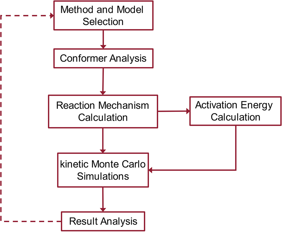
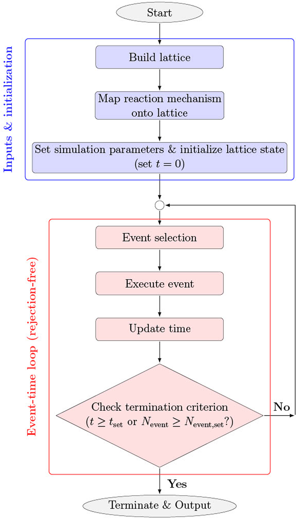
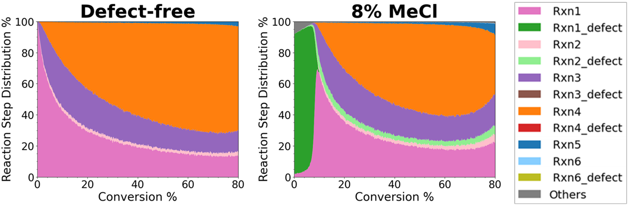
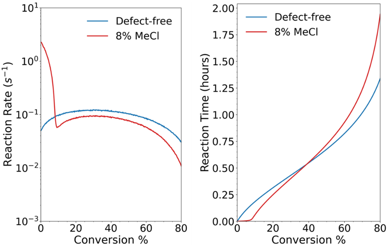
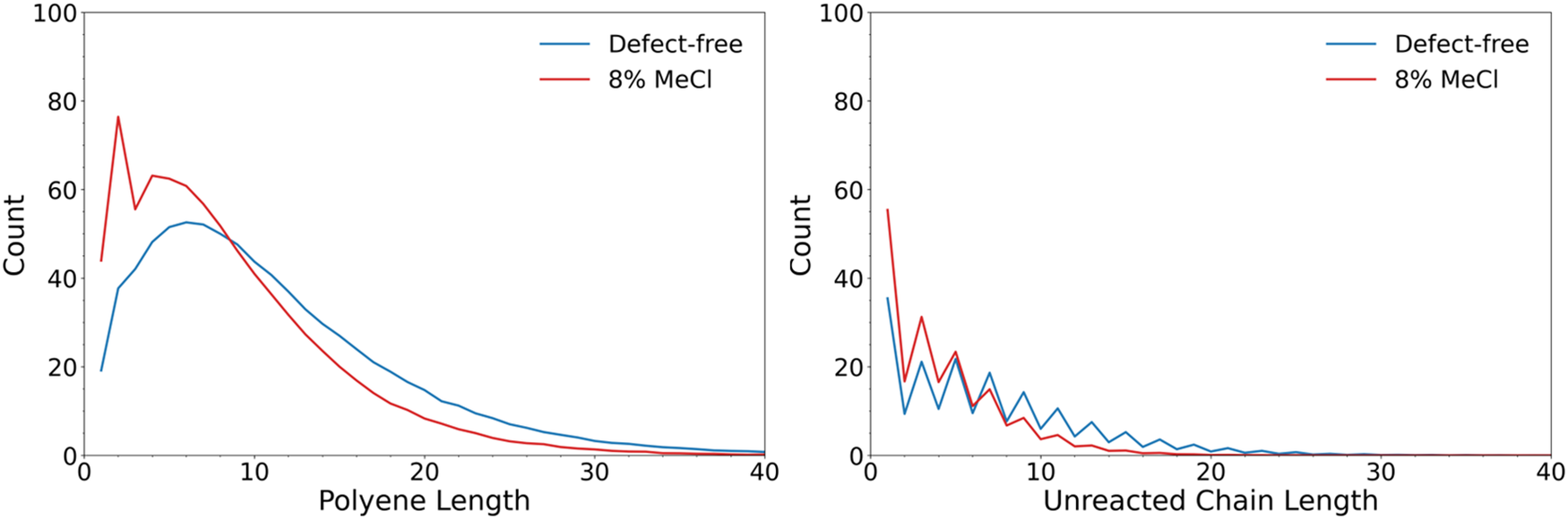


 Open access


Comments
March 20, 2026
Veena Sahajwalla
Editor-in-Chief
Cambridge Materials: Circularity
Dear Professor Sahajwalla,
We would like to submit our manuscript entitled “Extending Graph-based Lattice Kinetic Monte Carlo Simulations to Polymer Transformations: Tutorial Perspective” for publication as a perspective in Cambridge Materials: Circularity. Our submission follows an invitation from David Hopwood, Senior Publisher at Cambridge University Press, who contacted us after reviewing our ChemRxiv preprint and encouraged submission to Cambridge Materials: Circularity.
Polymer transformations involve coupled kinetic and structural evolution across multiple length and time scales, which has limited the predictive capability of many existing computational approaches. Our manuscript presents a tutorial-style implementation of our MUltiscale SIimulation frameworK (MUSIK) that demonstrates how high-level coupled cluster-based energetics are systematically translated into graph-based lattice kinetic Monte Carlo simulations for polymer transformations. Using base-assisted dehydrochlorination of PVC as a case study, we show how statistically converged ensembles of kMC trajectories reproduce both mechanistic trends and product distributions reported in prior MUSIK studies, without parameter fitting. Our tutorial establishes recommended practices for quantum chemical modeling of polymer reactions, including method and model selection, conformer sampling, and calculation of activation energies and pre-exponential factors that define elementary reaction steps. It further provides guidance on lattice-based kMC model construction, including lattice definition, event mapping, and statistical convergence criteria. We show how to map elementary steps and associated rate parameters onto a graph-based lattice to perform statistically converged kMC simulations under experimentally relevant conditions. We also disclose python-based post-processing procedures to extract kinetic and structural observables. By providing fully documented input construction, execution, and post-processing workflows, the manuscript lowers the barrier for applying MUSIK-based kMC simulations to new polymer systems and transformations.
We expect this work to serve as a reference point for researchers interested in performing predictive, multiscale simulations for polymer transformations. Cambridge Materials: Circularity focuses on sustainable materials systems and circular economies, including waste and recycling innovation, responsible production, and re-manufacturing. Our manuscript aligns with the journal’s scope by introducing a predictive multiscale framework for polymer transformations that enables mechanistic analysis of reaction pathways relevant to polymer degradation and recycling processes. By providing a fully documented tutorial perspective of MUSIK, we believe this manuscript will be of broad value to the readership of Cambridge Materials: Circularity.
The manuscript, or its contents in some other form, has not been published previously by any of the authors and is not under consideration for publication in another journal at the time of submission.
Following, we suggest the referees who can provide unbiased reviews on our manuscript. Suggested referees are not former mentors or mentees nor collaborators or coauthors from the past five years.
Thank you for your time and consideration.
Yours sincerely,
Tibor Szilvási
Recommended Reviewers
Linda Broadbelt Michail Stamatakis
Northwestern University University of Oxford
broadbelt@northwestern.edu michail.stamatakis@chem.ox.ac.uk
Dionisios G. Vlachos Dagmar R. D’hooge
University of Delaware Ghent University
vlachos@udel.edu dagmar.dhooge@ugent.be
Sribala Gorugantu Daniele Dini
University of Houston Imperial College London
sgorugantu@uh.edu d.dini@imperial.ac.uk
Gabriel G. B. Alves Alexander Shaw
São Paulo State University Northwestern University
carlos.graeff@unesp.br alexander.shaw@northwestern.edu
Gaurav Deshmukh Piaoping Yang
Northwestern University University of Delaware
spbatchu@northwestern.edu yangpp@udel.edu
Tej Choksi Heather J. Kulik
Nanyang University Massachusetts Institute of Technology
tej.choksi@ntu.edu.sg hjkulik@mit.edu
Reid Van Lehn
University of Wisconsin-Madison
ahensley@stevens.edu