1 Introduction
Oceanic internal solitary waves of large amplitude are often generated by the action of tidal currents over bottom topography and have been observed frequently in many coastal regions. The simplest model to describe the propagation of internal solitary waves is the weakly nonlinear Korteweg–de Vries (KdV) equation (Benjamin Reference Benjamin1966), where the effects of nonlinear wave steepening and linear wave dispersion are assumed to be balanced. Although the KdV model is widely used due to its simple form, its validity is rather limited to small-amplitude waves. For example, the KdV solitary wave is too narrow and moves too fast in comparison with laboratory or field observations (see Grue et al. Reference Grue, Jensen, Russ and Sveen1999). Higher-order weakly nonlinear models have also been proposed by including higher-order nonlinear and/or dispersive terms (see, for example, Koop & Butler Reference Koop and Butler1981). These models provide improved comparisons with observations, but, due to the weakly nonlinear assumption in their derivation, fail to capture a number of characteristics of large-amplitude internal solitary waves.
To take into account strong nonlinearity of large-amplitude internal solitary waves, for a two-layer system bounded above by a rigid surface, Miyata (Reference Miyata, Horikawa and Maruo1988) and Choi & Camassa (Reference Choi and Camassa1999) derived a theoretical model by assuming that the characteristic wavelength is long compared with the total fluid depth, but the wave amplitude is comparable to the total fluid depth. This strongly nonlinear long-wave model is often referred to as the MCC model in the literature and is an unsteady generalization of the steady long-wave model of Miyata (Reference Miyata1985). In comparison with laboratory experiments, it has been shown that the MCC model derived under the rigid-lid approximation successfully describes the propagation of large-amplitude internal solitary waves in two-layer settings (Choi & Camassa Reference Choi and Camassa1999; Camassa et al. Reference Camassa, Choi, Michallet, Rusas and Sveen2006).
In the majority of previous theoretical studies of internal solitary waves, it is common to assume that the top surface is rigid under the so-called rigid-lid approximation. When the density difference between two neighbouring layers is relatively small, for example as in oceanic conditions, it can be shown that the ratio between the displacement of the top free surface and that of the interface is proportional to the density jump (see § 2). In laboratory experiments where fresh water and brine were used for stratification (Segur & Hammack Reference Segur and Hammack1982; Kao, Pan & Renouard Reference Kao, Pan and Renouard1985; Grue et al. Reference Grue, Jensen, Russ and Sveen1999), the density difference and, therefore, the displacement of the top free surface were small, so that it was reasonable to compare the laboratory experiments with a model under the rigid-lid approximation. On the other hand, in some laboratory experiments (Walker Reference Walker1973; Koop & Butler Reference Koop and Butler1981; Michallet & Barthelemy Reference Michallet and Barthelemy1998), the density differences were non-negligible, but most comparisons of their measurements were made with theoretical models under the rigid-lid approximation and little attention was paid to the free surface. Theoretically, Moni & King (Reference Moni and King1995) studied the steady Euler equations for a two-layer system with a free surface, but computed only surface solitary wave solutions, while Peters & Stoker (Reference Peters and Stoker1960) considered weakly nonlinear solitary waves using the KdV model. To the best of our knowledge, large-amplitude internal solitary waves propagating under the top free surface in a two-layer system of constant densities have not been investigated systematically yet. In addition, it is important to allow the top surface to be free when the interaction of internal solitary waves with relatively short surface waves is investigated to better understand their surface expressions appearing on satellite images (Liu et al. Reference Liu, Chang, Hsu and Liang1998).
In this paper, free-surface effects on large-amplitude internal solitary waves are examined experimentally in a system of two immiscible fluids with a non-negligible density jump, and the measurements are compared with the strongly nonlinear model valid for the case when the top boundary is free (Choi & Camassa Reference Choi and Camassa1996; Barros, Gavrilyuk & Teshukov Reference Barros, Gavrilyuk and Teshukov2007), which is the generalization of the MCC model. In particular, we focus on the change in internal solitary wave profiles in the presence of the top free surface and the appearance of short surface wave packets above the internal solitary waves.
This paper is organized as follows. The model equations for internal solitary waves are presented in § 2. After describing the configuration of laboratory experiments in § 3, the measured wave profiles and wave speed of the internal solitary waves are compared with the theoretical solutions in § 4. Short surface wave packets observed during some of the laboratory experiments are described and their generation mechanisms are discussed in § 5. Then, concluding remarks are given in § 6.
2 Model equation
Consider a system of two fluid layers whose densities and thicknesses are given by
 $\unicode[STIX]{x1D70C}_{i}$
and
 $h_{i}$
respectively, with
 $i=1$
for the upper fluid layer and
 $i=2$
for the lower layer. When the characteristic wavelength
 $\unicode[STIX]{x1D706}$
is long compared with the total fluid depth so that
 $\unicode[STIX]{x1D716}=(h_{1}+h_{2})/\unicode[STIX]{x1D706}\ll 1$
, the strongly nonlinear models can be derived when the top surface is either rigid (Miyata Reference Miyata, Horikawa and Maruo1988; Choi & Camassa Reference Choi and Camassa1999) or free (Choi & Camassa Reference Choi and Camassa1996; Barros et al.
Reference Barros, Gavrilyuk and Teshukov2007).
2.1 The MCC-RL model
The MCC model under the rigid-lid assumption can be written, in terms of four unknowns (
 $\unicode[STIX]{x1D701}$
,
 $\overline{u}_{1}$
,
 $\overline{u}_{2}$
,
 $P$
), as
 $$\begin{eqnarray}\displaystyle & \displaystyle {\unicode[STIX]{x1D702}_{i}}_{t}+(\unicode[STIX]{x1D702}_{i}\overline{u}_{i})_{x}=0, & \displaystyle\end{eqnarray}$$
 $$\begin{eqnarray}\displaystyle & \displaystyle {\overline{u}_{i}}_{t}+\overline{u}_{i}{\overline{u}_{i}}_{x}+g\unicode[STIX]{x1D701}_{x}=-\frac{P_{x}}{\unicode[STIX]{x1D70C}_{i}}+\frac{1}{\unicode[STIX]{x1D702}_{i}}\left(\frac{1}{3}{\unicode[STIX]{x1D702}_{i}}^{3}G_{i}\right)_{x}, & \displaystyle\end{eqnarray}$$
where
 $\unicode[STIX]{x1D701}$
is the elevation of the interface,
 $P$
is the pressure at the interface, and
 $\overline{u}_{i}$
 $(i=1,2)$
are the depth-averaged horizontal velocities, defined by
 $$\begin{eqnarray}\overline{u}_{i}(x,t)=\frac{1}{\unicode[STIX]{x1D702}_{i}}\int _{[\unicode[STIX]{x1D702}_{i}]}u_{i}(x,z,t)\,\text{d}z,\end{eqnarray}$$
with
 $\int _{[\unicode[STIX]{x1D702}_{i}]}$
denoting
 $\int _{\unicode[STIX]{x1D701}}^{h_{1}}$
or
 $\int _{-h_{2}}^{\unicode[STIX]{x1D701}}$
for
 $i=1$
or 2 respectively. Here,
 $g$
is the gravitational acceleration,
 $\unicode[STIX]{x1D702}_{i}$
are the local layer thicknesses defined by
 $$\begin{eqnarray}\unicode[STIX]{x1D702}_{1}=h_{1}-\unicode[STIX]{x1D701},\quad \unicode[STIX]{x1D702}_{2}=h_{2}+\unicode[STIX]{x1D701}\end{eqnarray}$$
and
 $G_{i}$
are given by
 $$\begin{eqnarray}G_{i}(x,t)={\overline{u}_{i}}_{xt}+\overline{u}_{i}{\overline{u}_{i}}_{xx}-({\overline{u}_{i}}_{x})^{2}=-\frac{({D_{i}}^{2}\unicode[STIX]{x1D702}_{i})}{\unicode[STIX]{x1D702}_{i}},\end{eqnarray}$$
where
 $D_{i}\equiv \unicode[STIX]{x2202}_{t}+\overline{u}_{i}\unicode[STIX]{x2202}_{x}$
and we have used (2.1) for the last equality. The kinematic equations given by (2.1) are exact while the dynamic equations given by (2.2) have an error of
 $O(\unicode[STIX]{x1D716}^{4})$
. To distinguish it from the free-surface model introduced in the following section, the system for a top rigid lid given by (2.1)–(2.2) will be referred to as MCC-RL.
When a solitary wave is assumed to propagate, without change of form, with constant speed
 $c$
, one can write
 $\unicode[STIX]{x1D702}_{i}$
and
 $u_{i}$
, in the frame of reference moving with the solitary wave, as
 $$\begin{eqnarray}\unicode[STIX]{x1D702}_{i}=\unicode[STIX]{x1D702}_{i}(X),\quad \overline{u}_{i}=\overline{u}_{i}(X),\quad X=x-ct.\end{eqnarray}$$
After substituting (2.6) into (2.1), integrating the resulting equation once with respect to
 $X$
, and imposing the boundary conditions at infinities (
 $\unicode[STIX]{x1D702}_{1}\rightarrow h_{1}$
,
 $\unicode[STIX]{x1D702}_{2}\rightarrow h_{2}$
and
 $\overline{u}_{i}\rightarrow 0$
as
 $X\rightarrow \pm \infty$
),
 $\overline{u}_{i}$
can be expressed in terms of
 $\unicode[STIX]{x1D702}_{i}$
as
 $$\begin{eqnarray}\overline{u}_{i}=c\left(1-\frac{h_{i}}{\unicode[STIX]{x1D702}_{i}}\right).\end{eqnarray}$$
Then, after eliminating
 $P$
from (2.2) for
 $i=1,2$
and substituting (2.7) for
 $\overline{u}_{i}$
into the resulting equation, one can obtain a single nonlinear ordinary differential equation for
 $\unicode[STIX]{x1D701}$
(Miyata Reference Miyata1985):
 $$\begin{eqnarray}{\unicode[STIX]{x1D701}_{X}}^{2}=\frac{3\unicode[STIX]{x1D701}^{2}[c^{2}(\unicode[STIX]{x1D70C}_{1}\unicode[STIX]{x1D702}_{2}+\unicode[STIX]{x1D70C}_{2}\unicode[STIX]{x1D702}_{1})-g(\unicode[STIX]{x1D70C}_{2}-\unicode[STIX]{x1D70C}_{1})\unicode[STIX]{x1D702}_{1}\unicode[STIX]{x1D702}_{2}]}{c^{2}(\unicode[STIX]{x1D70C}_{1}{h_{1}}^{2}\unicode[STIX]{x1D702}_{2}+\unicode[STIX]{x1D70C}_{2}{h_{2}}^{2}\unicode[STIX]{x1D702}_{1})}.\end{eqnarray}$$
From
 $\unicode[STIX]{x1D701}_{X}=0$
when
 $\unicode[STIX]{x1D701}=a$
, the relationship between the solitary wave speed
 $c$
and its amplitude
 $a$
is given (Choi & Camassa Reference Choi and Camassa1999) by
 $$\begin{eqnarray}\frac{c^{2}}{{c_{0}}^{2}}=\frac{(h_{1}-a)(h_{2}+a)}{h_{1}h_{2}-({c_{0}}^{2}/g)a},\end{eqnarray}$$
where linear long-wave speed
 $c_{0}$
is given by
 $$\begin{eqnarray}{c_{0}}^{2}=\frac{gh_{1}h_{2}(\unicode[STIX]{x1D70C}_{2}-\unicode[STIX]{x1D70C}_{1})}{\unicode[STIX]{x1D70C}_{1}h_{2}+\unicode[STIX]{x1D70C}_{2}h_{1}}.\end{eqnarray}$$
The solitary wave solution satisfying
 $\unicode[STIX]{x1D701}\rightarrow 0$
as
 $X\rightarrow \infty$
can be found, by integrating (2.8) numerically, up to the maximum wave amplitude
 $a_{m}$
and its corresponding speed
 $c_{m}$
given by
 $$\begin{eqnarray}a_{m}=\frac{h_{1}-h_{2}\sqrt{\unicode[STIX]{x1D70C}_{1}/\unicode[STIX]{x1D70C}_{2}}}{1+\sqrt{\unicode[STIX]{x1D70C}_{1}/\unicode[STIX]{x1D70C}_{2}}},\quad {c_{m}}^{2}=g(h_{1}+h_{2})\frac{1-\sqrt{\unicode[STIX]{x1D70C}_{1}/\unicode[STIX]{x1D70C}_{2}}}{1+\sqrt{\unicode[STIX]{x1D70C}_{1}/\unicode[STIX]{x1D70C}_{2}}}.\end{eqnarray}$$
2.2 The MCC-FS model
When the upper layer is bounded above by the top free surface located at
 $z=h_{1}+\unicode[STIX]{x1D701}_{1}$
and below by the interface located at
 $z=\unicode[STIX]{x1D701}_{2}$
, the strongly nonlinear model (MCC-FS) with error of
 $O(\unicode[STIX]{x1D716}^{4})$
is given (Choi & Camassa Reference Choi and Camassa1996; Barros et al.
Reference Barros, Gavrilyuk and Teshukov2007) by
 $$\begin{eqnarray}{\unicode[STIX]{x1D702}_{1}}_{t}+(\unicode[STIX]{x1D702}_{1}\overline{u}_{1})_{x}=0,\quad \unicode[STIX]{x1D702}_{1}=h_{1}+\unicode[STIX]{x1D701}_{1}-\unicode[STIX]{x1D701}_{2},\end{eqnarray}$$
 $$\begin{eqnarray}{\unicode[STIX]{x1D702}_{2}}_{t}+(\unicode[STIX]{x1D702}_{2}\overline{u}_{2})_{x}=0,\quad \unicode[STIX]{x1D702}_{2}=h_{2}+\unicode[STIX]{x1D701}_{2},\end{eqnarray}$$
 $$\begin{eqnarray}\displaystyle & \displaystyle {\overline{u}_{1}}_{t}+\overline{u}_{1}{\overline{u}_{1}}_{x}+g(\unicode[STIX]{x1D702}_{1}+\unicode[STIX]{x1D702}_{2})_{x}=\frac{1}{\unicode[STIX]{x1D702}_{1}}\left(\frac{1}{3}{\unicode[STIX]{x1D702}_{1}}^{3}G_{1}\right)_{x}-\frac{1}{\unicode[STIX]{x1D702}_{1}}\left(\frac{1}{2}{\unicode[STIX]{x1D702}_{1}}^{2}{D_{1}}^{2}\unicode[STIX]{x1D702}_{2}\right)_{x} & \displaystyle \nonumber\\ \displaystyle & \displaystyle \hspace{78.0pt}+\,\left(\frac{1}{2}\unicode[STIX]{x1D702}_{1}G_{1}-{D_{1}}^{2}\unicode[STIX]{x1D702}_{2}\right){\unicode[STIX]{x1D702}_{2}}_{x}, & \displaystyle\end{eqnarray}$$
 $$\begin{eqnarray}\displaystyle & \displaystyle {\overline{u}_{2}}_{t}+\overline{u}_{2}{\overline{u}_{2}}_{x}+g(\frac{\unicode[STIX]{x1D70C}_{1}}{\unicode[STIX]{x1D70C}_{2}}\unicode[STIX]{x1D702}_{1}+\unicode[STIX]{x1D702}_{2})_{x}=\frac{1}{\unicode[STIX]{x1D702}_{2}}\left(\frac{1}{3}{\unicode[STIX]{x1D702}_{2}}^{3}G_{2}\right)_{x}\hspace{60.0pt} & \displaystyle \nonumber\\ \displaystyle & \displaystyle \hspace{150.0pt}+\,\frac{\unicode[STIX]{x1D70C}_{1}}{\unicode[STIX]{x1D70C}_{2}}\left(\frac{1}{2}{\unicode[STIX]{x1D702}_{1}}^{2}G_{1}-\unicode[STIX]{x1D702}_{1}{D_{1}}^{2}\unicode[STIX]{x1D702}_{2}\right)_{x}, & \displaystyle\end{eqnarray}$$
where
 $\overline{u}_{i}$
are the depth-averaged velocities defined by (2.3) with
 $\int _{[\unicode[STIX]{x1D702}_{i}]}$
defined as
 $\int _{\unicode[STIX]{x1D701}_{2}}^{h_{1}+\unicode[STIX]{x1D701}_{1}}$
or
 $\int _{-h_{2}}^{\unicode[STIX]{x1D701}_{2}}$
for
 $i=1$
or 2 respectively.
When the system given by (2.12)–(2.15) is linearized and its dispersive terms on the right-hand sides are neglected, one can obtain the linear long-wave speed
 $c_{0}$
by solving
 $$\begin{eqnarray}{c_{0}}^{4}-g(h_{1}+h_{2}){c_{0}}^{2}+g^{2}h_{1}h_{2}\left(1-\frac{\unicode[STIX]{x1D70C}_{1}}{\unicode[STIX]{x1D70C}_{2}}\right)=0,\end{eqnarray}$$
which yields the linear long-wave speeds of the faster barotropic (
 ${c_{0}}^{+}$
) and slower baroclinic (
 ${c_{0}}^{-}$
) modes. The ratio between the free-surface and interface displacements is given by
 $$\begin{eqnarray}\frac{\unicode[STIX]{x1D701}_{1}}{\unicode[STIX]{x1D701}_{2}}=\frac{{c_{0}}^{2}}{{c_{0}}^{2}-gh_{1}}.\end{eqnarray}$$
As it can be shown that
 $({c_{0}}^{-})^{2}<gh_{1}<({c_{0}}^{+})^{2}$
, the free surface and the interface are in phase
 $(\unicode[STIX]{x1D701}_{1}/\unicode[STIX]{x1D701}_{2}>0)$
for the barotropic mode while they are out of phase (
 $\unicode[STIX]{x1D701}_{1}/\unicode[STIX]{x1D701}_{2}<0$
) for the baroclinic mode.
For most previous experiments with
 $\unicode[STIX]{x1D6E5}=(\unicode[STIX]{x1D70C}_{2}-\unicode[STIX]{x1D70C}_{1})/\unicode[STIX]{x1D70C}_{2}\ll 1$
, the long-wave speeds can be approximated by
 $$\begin{eqnarray}(c_{0}^{+})^{2}=g(h_{1}+h_{2})\left[1-\frac{h_{1}h_{2}}{(h_{1}+h_{2})^{2}}\unicode[STIX]{x1D6E5}+O(\unicode[STIX]{x1D6E5}^{2})\right],\quad (c_{0}^{-})^{2}=\frac{gh_{1}h_{2}}{(h_{1}+h_{2})}\unicode[STIX]{x1D6E5}+O(\unicode[STIX]{x1D6E5}^{2}),\end{eqnarray}$$
where
 $\pm$
represent the barotropic and baroclinic internal-wave modes respectively. Then, the amplitude ratios for the two wave modes can be approximated, from (2.17), by
 $$\begin{eqnarray}\left(\frac{\unicode[STIX]{x1D701}_{1}}{\unicode[STIX]{x1D701}_{2}}\right)^{+}=\left(\frac{h_{1}+h_{2}}{h_{2}}\right)[1+O(\unicode[STIX]{x1D6E5})],\quad \left(\frac{\unicode[STIX]{x1D701}_{1}}{\unicode[STIX]{x1D701}_{2}}\right)^{-}=-\!\left(\frac{h_{2}}{h_{1}+h_{2}}\right)\unicode[STIX]{x1D6E5}[1+O(\unicode[STIX]{x1D6E5})].\end{eqnarray}$$
From (2.19), since
 $(\unicode[STIX]{x1D701}_{1}/\unicode[STIX]{x1D701}_{2})^{-}=O(\unicode[STIX]{x1D6E5})$
, the displacement of the top free surface can be neglected for the baroclinic mode for
 $\unicode[STIX]{x1D6E5}\ll 1$
, which most oceanic conditions satisfy. On the other hand, in our experiments,
 $\unicode[STIX]{x1D6E5}$
is not negligibly small (approximately 0.14), and the effect of the top free surface could be necessary in the description of the internal-wave motions. It should be noticed that this discussion about the free-surface effect should be applied to internal solitary waves in a two-layer system of constant densities. For example, it provides no explanation of the role of a top free surface on the instability of internal solitary waves observed previously in laboratory experiments (Grue et al.
Reference Grue, Jensen, Russ and Sveen2000; Carr et al.
Reference Carr, Fructus, Grue, Jensen and Davies2008; Luzzatto-Fegiz & Helfrich Reference Luzzatto-Fegiz and Helfrich2014) with linearly stratified fluids, in which recirculating cores could appear as the wave amplitude increases (Goullet & Choi Reference Goullet and Choi2008; Fructus et al.
Reference Fructus, Carr, Grue, Jensen and Davies2009). No internal solitary waves with such recirculating cores are possible in the two-layer system considered here.
For travelling solitary waves, in the frame of reference moving with wave speed
 $c$
as in (2.6), the system can be reduced to the following nonlinear system of coupled second-order differential equations (see appendix A for its derivation):
 $$\begin{eqnarray}\displaystyle \unicode[STIX]{x1D6FC}_{j1}\unicode[STIX]{x1D702}_{1}^{\prime \prime }+\unicode[STIX]{x1D6FC}_{j2}\unicode[STIX]{x1D702}_{2}^{\prime \prime }+\unicode[STIX]{x1D6FC}_{j3}{\unicode[STIX]{x1D702}_{1}^{\prime }}^{2}+\unicode[STIX]{x1D6FC}_{j4}{\unicode[STIX]{x1D702}_{2}^{\prime }}^{2}+\unicode[STIX]{x1D6FC}_{j5}\unicode[STIX]{x1D702}_{1}^{\prime }\unicode[STIX]{x1D702}_{2}^{\prime }=\unicode[STIX]{x1D6FC}_{j6}\quad \text{for }j=1,2, & & \displaystyle\end{eqnarray}$$
where the prime denotes differentiation with respect to
 $X$
and the nonlinear coefficients
 $\unicode[STIX]{x1D6FC}_{jk}$
can be found in appendix A. This steady system is identical to that obtained by Barros & Gavrilyuk (Reference Barros and Gavrilyuk2007) using the Lagrangian formulation. To find its solitary wave solutions, the system should be solved numerically for a given wave speed
 $c$
. While two different linear wave speeds (
 $c_{0}^{+}$
for barotropic waves and
 $c_{0}^{-}$
for baroclinic waves) are possible, internal solitary wave profiles are computed by choosing
 $c\rightarrow c_{0}^{-}$
in the limit of zero wave amplitude. Unlike the rigid-lid case, no explicit relationship between wave speed and wave amplitude is known and should be computed numerically.
2.3 The weakly nonlinear uni-directional model
For uni-directional waves, under the weakly nonlinear assumption, the MCC-RL and MCC-FS can be reduced to the KdV equation for the interface displacement
 $\unicode[STIX]{x1D701}_{2}$
(with
 $\unicode[STIX]{x1D701}_{2}=\unicode[STIX]{x1D701}$
for the rigid-lid case):
 $$\begin{eqnarray}{\unicode[STIX]{x1D701}_{2}}_{t}+c_{0}{\unicode[STIX]{x1D701}_{2}}_{x}+c_{1}\unicode[STIX]{x1D701}_{2}{\unicode[STIX]{x1D701}_{2}}_{x}+c_{2}{\unicode[STIX]{x1D701}_{2}}_{xxx}=0,\end{eqnarray}$$
where
 $c_{i}$
are given for the rigid-lid case by
 $$\begin{eqnarray}c_{1}=\frac{-3c_{0}}{2}\frac{\unicode[STIX]{x1D70C}_{1}{h_{2}}^{2}-\unicode[STIX]{x1D70C}_{2}{h_{1}}^{2}}{\unicode[STIX]{x1D70C}_{1}h_{1}{h_{2}}^{2}+\unicode[STIX]{x1D70C}_{2}{h_{1}}^{2}h_{2}},\quad c_{2}=\frac{c_{0}}{6}\frac{\unicode[STIX]{x1D70C}_{1}{h_{1}}^{2}h_{2}+\unicode[STIX]{x1D70C}_{2}h_{1}{h_{2}}^{2}}{\unicode[STIX]{x1D70C}_{1}h_{2}+\unicode[STIX]{x1D70C}_{2}h_{1}},\end{eqnarray}$$
while they are given for the free-surface case by
 $$\begin{eqnarray}\displaystyle & \displaystyle c_{1}=\frac{3c_{0}}{2h_{2}}\frac{1+(\unicode[STIX]{x1D70C}_{1}/\unicode[STIX]{x1D70C}_{2})h_{1}{h_{2}}^{2}/({c_{0}}^{2}/g-h_{1})^{3}}{1+(\unicode[STIX]{x1D70C}_{1}/\unicode[STIX]{x1D70C}_{2})h_{1}h_{2}/({c_{0}}^{2}/g-h_{1})^{2}}, & \displaystyle\end{eqnarray}$$
 $$\begin{eqnarray}\displaystyle & \displaystyle c_{2}=\frac{c_{0}{h_{2}}^{2}}{6}\frac{1+(\unicode[STIX]{x1D70C}_{1}/\unicode[STIX]{x1D70C}_{2})(h_{1}/h_{2})[3+3h_{1}/({c_{0}}^{2}/g-h_{1})+{h_{1}}^{2}/({c_{0}}^{2}/g-h_{1})^{2}]}{1+(\unicode[STIX]{x1D70C}_{1}/\unicode[STIX]{x1D70C}_{2})h_{1}h_{2}/({c_{0}}^{2}/g-h_{1})^{2}}.\qquad & \displaystyle\end{eqnarray}$$
 $$\begin{eqnarray}\unicode[STIX]{x1D701}_{2}(X)=a\text{sech}^{2}(X/\unicode[STIX]{x1D706}_{KdV}),\quad X=x-c_{KdV}t,\end{eqnarray}$$
where the characteristic length scale
 $\unicode[STIX]{x1D706}_{KdV}$
and the wave speed
 $c_{KdV}$
are given, respectively, by
 $$\begin{eqnarray}{\unicode[STIX]{x1D706}_{KdV}}^{2}=12c_{2}/(ac_{1}),\quad c_{KdV}=c_{0}+c_{1}a/3.\end{eqnarray}$$
3 Laboratory experiments
3.1 Two-fluid system
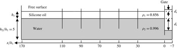
An immiscible two-fluid system is set up in an approximately 8.5 m long, 0.47 m wide and 0.35 m deep water tank in the Korea Advanced Institute of Science and Technology (KAIST). The bottom layer is a 0.25 m thick water layer and the top layer is a 0.05 m thick silicone oil layer. When necessary, physical variables are non-dimensionalized with respect to the top layer thickness
 $h_{1}$
and the gravitational acceleration
 $g$
. A vertical gate is installed 0.35 m away from one end of the tank in order to generate internal solitary waves by lifting the gate. The profiles of internal solitary waves are measured using five capacitance-type wave probes. The experimental configuration is schematically shown in figure 1.
Experimental set-up for the internal solitary wave generation in a two-fluid system with a free surface. The top layer is filled with the silicone oil SF1000NFC150 and the bottom layer is filled with water. The top layer thickness is
 $h_{1}=0.05~\text{m}$
while the lower layer thickness is
 $h_{2}=0.25~\text{m}$
. The specific gravities of silicone oil and water are denoted by
 $\unicode[STIX]{x1D70C}_{1}$
and
 $\unicode[STIX]{x1D70C}_{2}$
respectively. Five capacitance-type probes represented by black vertical lines are installed at a regular interval of 20 non-dimensional lengths. To generate internal solitary waves of five different wave amplitudes, the interface displacement is adjusted to
 $d_{i}/h_{1}=0.6$
, 1.2, 1.8, 2.4 and 3.0.

The kinematic viscosity of the silicone oil SF1000NFC150 used in the experiment is only 1.5 times greater than that of water based on the material safety data sheet, and we assume that the inviscid assumption can be used in modelling our experiments. The specific densities of the silicone oil and water are measured using a density meter. The specific gravity of the oil is
 $0.856\pm 0.001$
and that of the water is
 $0.996\pm 0.002$
at a temperature of
 $15\pm 1\,^{\circ }\text{C}$
. Therefore, the dimensionless density difference
 $\unicode[STIX]{x1D6E5}$
defined by
 $\unicode[STIX]{x1D6E5}=(\unicode[STIX]{x1D70C}_{2}-\unicode[STIX]{x1D70C}_{1})/\unicode[STIX]{x1D70C}_{2}$
is approximately 0.14. The fluctuation of specific density of each fluid is due to either thermal expansion of the fluid or the measurement error mainly caused by the meniscus effect on the wall of the density meter.
With the current experimental set-up with the top free surface, the phase speed of linear long internal waves is given, from (2.16), by
 $c_{0}=0.242~\text{m}~\text{s}^{-1}$
. If the top boundary is rigid, the phase speed increases to
 $0.255~\text{m}~\text{s}^{-1}$
. The difference between the two phase speeds is approximately 5 % of
 $c_{0}$
, which cannot be neglected for the phase speed measurement.
3.2 Internal solitary wave generation
The method to generate internal solitary waves is the same as that of Michallet & Barthelemy (Reference Michallet and Barthelemy1998). By adjusting the interfacial displacement
 $d_{i}$
behind the gate, internal solitary waves of a wide range of amplitudes are generated (figure 1). Since the gate is not fully closed to the bottom before the gate is lifted, the water can flow freely below the gate. As a result, the surface behind the gate rises to balance the bottom pressure difference produced by the displaced interface behind the gate. As long as the system is hydrostatically balanced, the surface elevation
 $d_{s}$
is estimated to be
 $$\begin{eqnarray}d_{s}=\left(\frac{\unicode[STIX]{x1D70C}_{2}-\unicode[STIX]{x1D70C}_{1}}{\unicode[STIX]{x1D70C}_{1}+\unicode[STIX]{x1D70C}_{2}}\right)d_{i}.\end{eqnarray}$$
The estimation based on the isostasy (3.1) agrees well with the values measured before the experiments start. Five different interface displacements
 $d_{i}/h_{1}=(0.6,1.2,1.8,2.4,3.0)$
are chosen and each experiment is repeated five times to reduce random experimental errors. Then, the wave amplitudes are determined from the measurements at the fifth wave probe by taking an average over the five repetitions. The emerging solitary wave amplitudes
 $a/h_{1}=(0.24,0.50,0.77,0.99,1.21)$
are used to name each experiment. For example, case 0.24 represents the experiment for the solitary wave whose dimensionless amplitude is 0.24.
The gate is not completely pulled out of the oil layer, but stopped just below the top free surface to minimize the generation of barotropic surface waves. Nevertheless, small-amplitude surface waves are always observed. They propagate faster than the internal waves and are reflected back from the end of the tank. To avoid any possible contamination of internal solitary wave measurements, the reflection of fast-propagating small-amplitude surface waves is suppressed by loose nets, as wave absorbers, placed at the end of the tank.
3.3 Measurement techniques
The generated internal solitary waves are measured by capacitance-type wave probes with a sampling frequency of 200 Hz. The capacitance-type wave probe was originally designed to measure the displacement of the air–water interface, and care should be taken for the oil–water interface. A previous experimental study (Walker Reference Walker1973) with Humble oil (Varsol I) and water neglected any influence of the oil on the wave probe measurement because the wave probe was 550 times less sensitive to the Humble oil than water. On the other hand, our wave probes are on average only 31 times less sensitive to the silicone oil than to the water.
To take into account the influence of the silicone oil on the internal displacement estimation, we use the following formula to determine the interface displacement
 $\unicode[STIX]{x1D701}_{2}$
from the output voltage
 $V$
of the wave probe:
 $$\begin{eqnarray}V=C_{w}\unicode[STIX]{x1D701}_{2}+C_{o}(\unicode[STIX]{x1D701}_{1}-\unicode[STIX]{x1D701}_{2}),\end{eqnarray}$$
where
 $C_{w}$
and
 $C_{o}$
are the calibration coefficients for water and silicone oil respectively, and
 $\unicode[STIX]{x1D701}_{1}$
is the surface displacement. After using (2.17) to estimate the ratio between
 $\unicode[STIX]{x1D701}_{1}$
and
 $\unicode[STIX]{x1D701}_{2}$
, the interfacial displacement
 $\unicode[STIX]{x1D701}_{2}$
can be determined from (3.2) for the given output voltage
 $V$
. The second term on the right-hand side of (3.2) is smaller than the first term as
 $C_{o}\ll C_{w}$
, as stated above. The resultant difference of the interface displacement
 $\unicode[STIX]{x1D701}_{2}$
is 3.65 % on average when the effect of the upper oil layer is included.
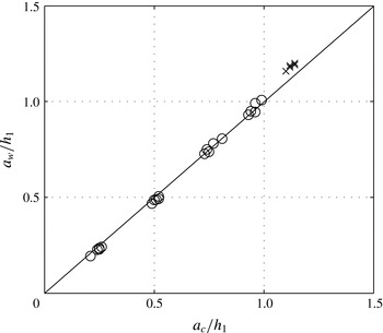
The accuracy of the measured displacements based on (2.17) and (3.2) is verified with another independent measurement using a digital camera that is placed in front of the third wave probe located at
 $x/h_{1}=70$
. The wave amplitude is read from the images captured by the camera within a possible error of 0.5 mm, or 1 % of the top layer thickness. A ruler is also positioned inside the tank to take into account optical refraction by the glass wall. As a result, little discrepancy is found between the measured amplitudes using the two different methods (figure 2).
Comparison between the wave amplitudes measured at
 $x/h_{1}=70$
by a digital camera,
 $a_{c}$
, and by a wave probe,
 $a_{w}$
. The
 $\times$
marks are for case 1.21 in which the internal solitary waves are perturbed greatly by the Kelvin–Helmholtz instability.

3.4 Measurement errors
Both random noise and bias may contaminate experimental data. The device-originated mechanical noise is reduced by taking a running average over 20 sample points, whose time duration is 0.1 s. Other random noise may be produced by imperfectly set interface levels behind the gate and manual lifting of the gate. The random noise is reduced by taking the average over five repeated measurements for each configuration. However, bias is not removed by this averaging process.
Possible factors to produce bias are the thermal expansion of the two fluids during the experiments and the installed position of the sensing wires. The thermal expansion mainly influences the internal solitary wave speed. The linear phase speed of internal waves increases by, at most, 0.99 % when the specific gravity of the oil changes from 0.856 to 0.855 and the specific gravity of the water changes from 0.996 to 0.998. The position of a sensing wire also has an error of 0.01 m due to technical difficulties in its installation. The expected error in the phase speed from the installation position is estimated to be approximately 1 %. Since the error is smaller than the differences between the various theoretical models used for the comparison, the measurements are considered to be reliable to determine the validity of the theoretical models.
4 Results
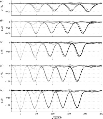
Measured interfacial displacements at the five wave probes, non-dimensionalized by the top layer thickness
 $h_{1}$
: (a) case 0.24, (b) case 0.50, (c) case 0.77, (d) case 0.99 and (e) case 1.21. The dimensionless time for each case is set to zero when the first wave probe records the largest displacement. The lines represent experimental data with changing colours from light grey to black for the first to fifth wave probes.

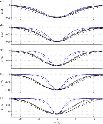
Comparison of internal solitary wave profiles between experiments and theoretical models: (a) case 0.24, (b) case 0.50, (c) case 0.77, (d) case 0.99 and (e) case 1.21. The profiles are non-dimensionalized by using the top layer thickness
 $h_{1}$
and each wave speed
 $c$
measured by the fourth and fifth wave probes. Circles, experimental data averaged over the five repetitions; black line, MCC-FS; black dashed line, MCC-RL; blue line, KdV-FS; blue dashed line, KdV-RL.

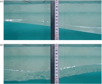
An internal solitary wave recorded by a digital camera during the experiment of case 1.21 for (a) the front half and (b) the rear half (i.e. the solitary wave propagates to the left). The pictures are taken just in front of the third wave probe located at
 $x/h_{1}=70$
. The ruler in cm shown in the figure shows the spatial scale of the internal-wave motion. The appearance of short surface waves on the top free surface can also be observed on the top of snapshot (a) and is discussed in § 5.

4.1 Wave profiles
As the gate is lifted, the initially displaced interface disintegrates into a leading solitary wave and a dispersive tail, as shown in figure 3. Comparison between the five repeated measurements shown in each panel of figure 3 indicates that the experiments are repeatable. Then, the measured wave profiles are averaged over five repetitions by specifying the maximum correlation coefficient with one of the five records. Leading solitary waves are clearly detected even by the first wave probe without any significant contamination from dispersive tails. The amplitude of the leading solitary wave is then observed to decrease as it propagates downstream, in particular to the second wave probe, beyond which it remains approximately unchanged. The initial decrease of the amplitude implies that the solitary wave needs some time before it reaches a steady state. Theoretical wave profiles are hence compared with the measurement at the fifth wave probe to avoid the initially transient effects. As the wave amplitude increases, the leading solitary wave arrives earlier at wave probes located further downstream, as expected. The relationship between the wave amplitude and the speed will be discussed in detail in the following section.
For the smallest-amplitude case shown in figure 4(a), the averaged wave profile agrees well with the solitary wave solutions of the weakly nonlinear KdV-RL model and the strongly nonlinear MCC-FS model. On the other hand, the KdV-FS equation underestimates the interfacial displacement while the strongly nonlinear MCC-RL model overestimates it. As the amplitude increases (figure 4
b–d), the measured wave profiles consistently show good agreement only with the MCC-FS model. The solitary wave profiles from both the KdV-RL equation and the KdV-FS equation are narrower than the measured wave profiles, while the wave profiles from the MCC-RL model are broader. Therefore, it can be concluded that an internal solitary wave propagating under a top free surface is always narrower than that under a rigid lid, which has not been confirmed experimentally before. In addition, when the internal solitary wave propagates, it is observed that the top free surface is clearly displaced in the opposite direction to the interfacial displacement (see figure 5). Thus the free-surface boundary condition at the top surface is important to correctly describe the profiles of the internal solitary waves observed in our experiments even though the density difference (
 $\unicode[STIX]{x1D6E5}=0.14$
) is relatively small.
The wave profiles are almost symmetric for small and intermediate wave amplitudes in figure 4(a–c), but show some asymmetry, in particular, when the amplitude is almost comparable to the top layer thickness (figure 4 d,e). The asymmetry could be caused in part by the slight unsteadiness of the experiment, but it is pronounced in figure 4(e), where the internal solitary wave suffers from the Kelvin–Helmholtz (KH) instability excited by the large shear across the interface. Figure 5(b) for case 1.21 captures unstable short internal waves that appear on the rear part of the leading internal solitary wave, while the front part shown in figure 5(a) is smooth. A similar observation was made in the salt water experiment of Grue et al. (Reference Grue, Jensen, Russ and Sveen1999). It should be pointed out that the surface tension between the two immiscible fluids (oil and water) is non-negligible and plays a stabilizing role when the KH instability is excited. Therefore, in contrast to previous experiments with salt water, no overturning KH billows are observed. This implies that the shear induced across the interface by an internal solitary wave is finite, but is not large enough to overcome the surface tension effect. While three-dimensional disturbances are observed, as shown in figure 5(b), the wave probe measurements are taken along the centreline of the tank. We should also remark that, while short-wavelength disturbances on the interface are excited initially when the gate is lifted, they are hardly observed as the internal solitary waves of small or intermediate wave amplitude propagate downstream.
4.2 Wave speed
The wave speed of the leading internal solitary wave is determined based on the time interval between its arrival at two adjacent wave probes. The interval is determined to maximize the cross-correlation between the two time series. Since there are five wave probes, the wave speed is estimated at four locations (i.e.,
 $x/h_{1}=40$
, 60, 80 and 100). The amplitudes at the four locations are determined as an average of the amplitudes measured by two adjacent wave probes. The relationship between wave speed and wave amplitude is shown in figure 6 for five different cases. As observed previously from the wave profile measurements, figure 6 again shows that the leading solitary wave is significantly attenuated after it is released from the gate, but remains almost unchanged after it passes the third wave probe. The initial decrease of wave amplitude over the first two wave probe locations is greater than the standard deviation of the five repeated measurements, but, after the leading wave passes the third wave probe, the variation of wave amplitude and wave speed is comparable to the standard deviation.
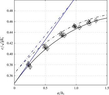
Measured wave speed
 $c$
versus wave amplitude
 $a$
of internal solitary waves, non-dimensionalized by
 $\sqrt{gh_{1}}$
and
 $h_{1}$
respectively: ♢, data from the first and second wave probes;
 $\times$
, data from the second and third wave probes; △, data from the third and fourth wave probes; ○, data from the fourth and fifth wave probes. The error bars denoted by the short horizontal and vertical lines on top of symbols represent the standard deviations of five repeated measurements for the wave amplitude and the wave speed respectively. Black line, MCC-FS; black dashed line, MCC-RL; blue solid line, KdV-FS; blue dashed line, KdV-RL.

The measured relationship between wave speed and wave amplitude is compared with various theoretical models in figure 6. The weakly nonlinear models obviously overestimate the wave speeds of large-amplitude internal solitary waves. As the experimental data for intermediate wave amplitudes lie between the two strongly nonlinear MCC models, it is difficult to draw a conclusion on the validity of the two strongly nonlinear models in terms of wave speed measurements. For our experimental set-up, the difference in wave speed between the rigid-lid and free-surface cases is theoretically as large as 5 % for small-amplitude waves, but decreases to approximately 1.5 % for large-amplitude waves, which is comparable to the possible measurement error, which was estimated to be at most 2 % in § 3.4. Nevertheless, a significant discrepancy from the rigid-lid model can be clearly observed for smaller-amplitude cases, for example case 0.26. Since its agreement with the wave speed measurements along with our observation of wave profiles is noticeable for a wide range of wave amplitudes, the strongly nonlinear MCC-FS model is relevant for our experiments with the top free surface.
5 Short surface waves above internal solitary waves
When the amplitude of an internal solitary wave is relatively large (
 $a/h_{1}\geqslant 0.77$
), short surface waves are often observed on the top free surface, approximately right above the front half of the internal solitary wave, not right above or behind the trough of maximal displacement. The short surface waves form a wave packet with a representative wavelength of 3–4 cm, as shown in figure 5(a), The corresponding dimensionless wavelength and wavenumber are
 $\unicode[STIX]{x1D706}_{obs}/h_{1}=0.6\sim 0.8$
and
 $k_{obs}h_{1}=7.85\sim 10.47$
respectively. No noticeable surface waves are detected on the free surface above the rear half of the solitary wave (figure 5
b). The propagation of the short surface waves is recorded by a camcorder placed at
 $x/h_{1}=70$
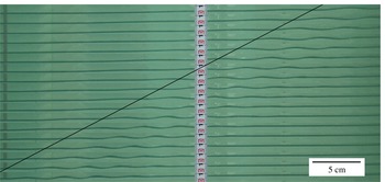
. It is difficult to measure the propagation speed of the surface wave packet precisely, but its speed is found to be approximately close to the wave speed of the internal solitary wave, as indicated by the straight line in figure 7. Therefore, one can imagine that the short surface waves are possibly generated by some action of the internal solitary wave.
Combined snapshots of short surface waves recorded by a camcorder placed at
 $x/h_{1}=70$
for case 1.21. The snapshots were taken at every
 $4/60$
s and the first snapshot is placed at the top of the picture. The straight line whose slope is the same as the internal solitary wave speed is added to show that the surface wave packet is propagating with the internal solitary wave.

To study the propagation of the short surface waves, we consider an internal solitary wave of
 $a/h_{1}=1.21$
, for which the appearance of short surface waves is most evident. For an internal solitary wave of this wave amplitude travelling to the left, the wave speed is
 $c/(gh_{1})^{1/2}\simeq 0.450$
from the MCC-FS model, while its linear long-wave speed is
 $c_{0}/(gh_{1})^{1/2}\simeq 0.340$
. It should be noticed that the solitary wave speed of the MCC-RL model is
 $c/(gh_{1})^{1/2}\simeq 0.456$
.
One possible scenario is a (linear) resonance mechanism between long internal waves and short surface waves, where the following condition is met:
 $$\begin{eqnarray}c_{0}^{-}=c_{g}^{+}.\end{eqnarray}$$
Here,
 $c_{0}^{-}$
is the linear long-internal-wave speed given by (2.16) and
 $c_{g}^{+}$
is the group velocity of (relatively) short surface waves, which can be found as described below. In a two-layer system with a top free surface, the wave frequency
 $\unicode[STIX]{x1D6FA}$
for gravity–capillary waves can be found from
 $$\begin{eqnarray}\displaystyle & (\unicode[STIX]{x1D70C}_{1}+\unicode[STIX]{x1D70C}_{2}\coth kh_{1}\coth kh_{2})\unicode[STIX]{x1D6FA}^{4}-k[\!\unicode[STIX]{x1D70C}_{1}{\hat{g}}_{1}\coth kh_{1}+\unicode[STIX]{x1D70C}_{2}{\hat{g}}_{1}\coth kh_{2} & \displaystyle \nonumber\\ \displaystyle & \quad +\,(\unicode[STIX]{x1D70C}_{2}-\unicode[STIX]{x1D70C}_{1}){\hat{g}}_{2}\coth kh_{1}\! ]\unicode[STIX]{x1D6FA}^{2}+(\unicode[STIX]{x1D70C}_{2}-\unicode[STIX]{x1D70C}_{1}){\hat{g}}_{1}{\hat{g}}_{2}k^{2}=0, & \displaystyle\end{eqnarray}$$
where
 $k$
is the wavenumber and
 ${\hat{g}}_{i}$
are given by
 $$\begin{eqnarray}{\hat{g}}_{1}=g\left(1+\frac{\unicode[STIX]{x1D6FE}_{1}}{\unicode[STIX]{x1D70C}_{1}g}k^{2}\right),\quad {\hat{g}}_{2}=g\left[1+\frac{\unicode[STIX]{x1D6FE}_{2}}{(\unicode[STIX]{x1D70C}_{2}-\unicode[STIX]{x1D70C}_{1})g}k^{2}\right],\end{eqnarray}$$
with
 $\unicode[STIX]{x1D6FE}_{1}$
and
 $\unicode[STIX]{x1D6FE}_{2}$
being the surface tension coefficients on the top free surface and the interface respectively. For the silicone oil used in the experiment, the surface tension coefficient at the top free surface is
 $\unicode[STIX]{x1D6FE}_{1}=0.018~\text{N}~\text{m}^{-1}$
(compared with
 $0.0728~\text{N}~\text{m}^{-1}$
for water) and the surface tension effect on short surface waves can be estimated as
 $$\begin{eqnarray}\unicode[STIX]{x1D6FE}_{1}k^{2}/\unicode[STIX]{x1D70C}_{1}g\simeq 0.053,\end{eqnarray}$$
where
 $k=2\unicode[STIX]{x03C0}/4~\text{cm}^{-1}$
, corresponding to the observed surface waves, has been used. Since this dimensionless parameter, or the inverse of the Weber number, is relatively small, the surface tension effect can be neglected. Then, the wave frequency for surface waves can be found from
 $$\begin{eqnarray}(\unicode[STIX]{x1D70C}_{1}+\unicode[STIX]{x1D70C}_{2}\coth kh_{1}\coth kh_{2})\unicode[STIX]{x1D6FA}^{4}-\unicode[STIX]{x1D70C}_{2}gk(\coth kh_{1}+\coth kh_{2})\unicode[STIX]{x1D6FA}^{2}+(\unicode[STIX]{x1D70C}_{2}-\unicode[STIX]{x1D70C}_{1})g^{2}k^{2}=0,\end{eqnarray}$$
whose solutions yield the following linear dispersion relations:
 $$\begin{eqnarray}{\unicode[STIX]{x1D6FA}_{\pm }}^{2}=\frac{gk}{2(1+\unicode[STIX]{x1D70C}T_{1}T_{2})}\left[T_{1}+T_{2}\pm \sqrt{(T_{1}+T_{2})^{2}-4T_{1}T_{2}(1-\unicode[STIX]{x1D70C})(1+\unicode[STIX]{x1D70C}T_{1}T_{2})}\right],\end{eqnarray}$$
where
 $\unicode[STIX]{x1D70C}=\unicode[STIX]{x1D70C}_{1}/\unicode[STIX]{x1D70C}_{2}<1$
,
 $T_{1}=\tanh (kh_{1})$
and
 $T_{2}=\tanh (kh_{2})$
. Here, the plus and minus signs correspond to the barotropic and baroclinic modes (or the surface-wave and internal-wave modes) respectively. With the group velocity of surface-mode waves
 ${c_{g}}^{+}=\unicode[STIX]{x2202}\unicode[STIX]{x1D6FA}_{+}/\unicode[STIX]{x2202}k$
, the wavenumber
 $k_{res}$
and the corresponding wavelength
 $\unicode[STIX]{x1D706}_{res}$
satisfying the linear resonance condition (
 $c_{0}^{-}=c_{g}^{+}$
) in (5.1) can be found as
 $k_{res}h_{1}\simeq 2.163$
and
 $\unicode[STIX]{x1D706}_{res}/h_{1}\simeq 2.904$
respectively. Alternatively, as it is relatively large, this resonant wavenumber can be estimated as
 $k_{res}h_{1}\approx gh_{1}/(2c_{0}^{-})^{2}$
from the dispersion relation for surface waves in deep water, for which the group velocity is given by
 $c_{g}^{+}=(1/2)(g/k)^{1/2}$
. Compared with the observed wavelength (
 $\unicode[STIX]{x1D706}_{obs}/h_{1}=0.6\sim 0.8$
), the resonant wave is too long, and, therefore, the linear resonance mechanism is apparently unable to describe the appearance of short surface waves.
As the large-amplitude internal solitary wave induces a significant surface current
 $u_{s}$
, the resonance condition accounting for the leading-order nonlinear effect might need to be modified to
 $$\begin{eqnarray}c=c_{g}^{+}+u_{s}.\end{eqnarray}$$
It should be noticed that the linear long-wave speed
 $c_{0}^{-}$
on the left-hand side of (5.1) is replaced by the speed of the solitary wave of MCC-FS, while the Doppler effect is included in estimating the group velocity of short surface waves. Under this modified resonance condition, the resonant wavenumber
 $k_{res}$
is approximated by
 $k_{res}h_{1}\approx gh_{1}/[2(c-u_{s})]^{2}$
. As the upper-layer horizontal velocity
 $u_{1}$
induced by the internal solitary wave varies in space,
 $u_{s}$
is estimated as the upper-layer horizontal velocity at the location of the maximum displacement of the interface (at
 $X=0$
), so that
 $u_{s}/(gh_{1})^{1/2}\simeq 0.261$
. Even for the top free-surface case, as can be seen from (2.12)–(2.13),
 $u_{1}$
can be computed from (2.7), although the definition of
 $\unicode[STIX]{x1D702}_{1}$
should be modified to
 $\unicode[STIX]{x1D702}_{1}=h_{1}+\unicode[STIX]{x1D701}_{1}-\unicode[STIX]{x1D701}_{2}$
, where
 $\unicode[STIX]{x1D701}_{1}/\unicode[STIX]{x1D701}_{2}\simeq -0.131$
from (2.17). Then, the resonant wavenumber and wavelength can be found as
 $k_{res}h_{1}\simeq 6.998$
and
 $\unicode[STIX]{x1D706}_{res}/h_{1}\simeq 0.898$
respectively. In comparison with the observed wavelengths (
 $\unicode[STIX]{x1D706}_{obs}/h_{1}=0.6\sim 0.8$
), the wavelength estimated by the modified resonant condition (5.7) gives a much better agreement. Nevertheless, it should be remarked that this result is based on a particular choice of
 $u_{s}$
, which is the horizontal velocity of the upper layer at the maximal displacement (
 $X=0$
). For example, if the resonance condition is satisfied away from
 $X=0$
where
 $u_{s}$
is found to be smaller, a longer wave could be excited. Therefore, it remains to be explained how the surface waves possibly excited by the resonance mechanism evolve as they propagate with the internal solitary wave.
Here, as in Donato, Peregrine & Stocker (Reference Donato, Peregrine and Stocker1999), ray theory is adopted to study the evolution of surface waves in a slowly varying current induced by an internal solitary wave. In the frame of reference moving with the internal solitary wave speed
 $c$
, the background surface current is given, as the leading-order approximation, by
 $U(X)=u_{1}(X)-c$
, so that
 $$\begin{eqnarray}U(X)=-c\,\frac{h_{1}}{\unicode[STIX]{x1D702}_{1}},\end{eqnarray}$$
where
 $X=x-ct$
. Then, the wave frequency of surface gravity waves in the moving frame is given by
 $$\begin{eqnarray}\unicode[STIX]{x1D714}(k,X)=U(X)k\pm \unicode[STIX]{x1D6FA}_{+}(k),\end{eqnarray}$$
where the plus (or minus) sign corresponds to the right-going (or left-going) waves in the absence of surface current. Due to the presence of non-uniform current, the wavenumber
 $k$
no longer remains constant. Instead, from
 $\unicode[STIX]{x2202}k/\unicode[STIX]{x2202}t+\unicode[STIX]{x2202}\unicode[STIX]{x1D714}/\unicode[STIX]{x2202}X=0$
, the evolution of the local wavenumber
 $k$
of surface gravity waves is governed by
 $$\begin{eqnarray}\frac{\unicode[STIX]{x2202}k}{\unicode[STIX]{x2202}t}+(U\pm c_{g}^{+})\frac{\unicode[STIX]{x2202}k}{\unicode[STIX]{x2202}X}+k\frac{\text{d}U}{\text{d}X}=0.\end{eqnarray}$$
Alternatively, along a ray path defined by
 $$\begin{eqnarray}\frac{\text{d}X}{\text{d}t}=U(X)\pm c_{g}^{+}=\frac{\unicode[STIX]{x2202}\unicode[STIX]{x1D714}}{\unicode[STIX]{x2202}k},\end{eqnarray}$$
equation (5.10) can be rewritten as
 $$\begin{eqnarray}\frac{\text{d}k}{\text{d}t}=-kU^{\prime }(X)=-\frac{\unicode[STIX]{x2202}\unicode[STIX]{x1D714}}{\unicode[STIX]{x2202}X}.\end{eqnarray}$$
Then, as
 $\unicode[STIX]{x2202}\unicode[STIX]{x1D714}/\unicode[STIX]{x2202}t=0$
from (5.9), the following holds for wave frequency
 $\unicode[STIX]{x1D714}$
:
 $$\begin{eqnarray}\frac{\text{d}\unicode[STIX]{x1D714}}{\text{d}t}=\frac{\unicode[STIX]{x2202}\unicode[STIX]{x1D714}}{\unicode[STIX]{x2202}k}\frac{\text{d}k}{\text{d}t}+\frac{\unicode[STIX]{x2202}\unicode[STIX]{x1D714}}{\unicode[STIX]{x2202}X}\frac{\text{d}X}{\text{d}t}=0,\end{eqnarray}$$
where (5.11) and (5.12) have been used. This implies that
 $\unicode[STIX]{x1D714}$
remains unchanged along any ray. Thus, if it is initially uniform in space, the wave frequency must be uniform in space at a later time. In such a situation, the frequency is therefore constant in both space and time. Then, the variation of the local wavenumber
 $k$
in
 $X$
for given
 $U(X)$
can be seen along the level curves of
 $\unicode[STIX]{x1D714}$
, or the curves of constant
 $\unicode[STIX]{x1D714}$
, given by (5.9), from which one can understand how short surface waves are modulated by the non-uniform background current
 $U(X)$
.
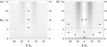
In figure 8, the level curves of
 $\unicode[STIX]{x1D714}$
given by (5.9) are shown for the right- and left-going surface waves. For the right-going waves (propagating in the direction opposite to that of the solitary wave in the fixed frame), they are shortened as they propagate through the current field induced by the solitary wave, but recover their original wavelengths as they propagate away from the internal solitary wave. On the other hand, for the left-going waves (propagating in the same direction as the internal solitary wave in the fixed frame), the change of the wavenumber is more substantial. The level curves originating from
 $x=-\infty$
in the moving frame show a sharp increase of the wavenumber as they approach the internal solitary wave, while the surface waves of small wavenumbers propagate much faster than the internal solitary wave so that they propagate to the left even in the moving reference frame with little interaction. It should be noticed that there are closed contours whose centres are located at
 $X/h_{1}=0$
and
 $kh_{1}\simeq 6.998$
, the critical points of (5.11) and (5.12). In fact, this is exactly the resonance condition at
 $X=0$
given by (5.7). The existence of such closed contours implies that, once surface waves are excited possibly through the resonance mechanism and located above the internal solitary wave, the wavenumber increases rapidly in the front half of the internal solitary wave where
 $U^{\prime }(X)<0$
. This shows the importance of the gradient of the surface current on the emergence of short surface wave packets.
As the wavenumber increases, the surface-wave amplitude is also expected to grow and, therefore, steep surface waves could be observed on the top surface located above the front half of the internal solitary wave, not right above or behind the wave trough, as mentioned previously. The location of a packet of short surface waves is consistent with our observation, but has not been clearly identified. Nevertheless, the appearance and the evolution of short surface waves still need to be investigated more systematically, but it should be remarked that the observed location of short surface waves is close to where the wavenumber increases rapidly. Moreover, if the surface waves become too steep, linear ray theory becomes invalid and the nonlinear effects have to be included for a complete explanation.
The level curves of
 $\unicode[STIX]{x1D714}$
given by (5.9) with the surface current induced by a solitary wave of
 $a/h_{1}=1.22$
. (a) Right-going surface waves, (b) left-going surface waves.

6 Conclusion
Internal solitary waves of large wave amplitudes have been studied experimentally in a system of two fluids, silicone oil and water, where the free-surface effects cannot be neglected due to a small but non-negligible density difference between the two fluids. The measured wave profiles and wave speeds using multiple wave probes are averaged over five repeated experiments to reduce measurement errors and are then validated with independent measurements using a digital camera. The measurements are also compared with both weakly nonlinear and strongly nonlinear long-internal-wave models with and without the rigid-lid assumption for the top surface. The weakly nonlinear KdV models show poor comparison for intermediate- and large-amplitude waves, while the strongly nonlinear MCC model with a rigid lid, often used for large-amplitude internal waves in a two-fluid system, predicts wider wave profiles. This discrepancy has been resolved by the MCC model with a free surface. As the density difference between the two fluids is non-negligible, it can be concluded that the top free surface has to be modelled correctly even for internal-wave motion.
When the wave amplitude is large, the rear half of the internal solitary wave suffers from the Kelvin–Helmholtz instability due to large shear across the interface, while the front half of the interface is smooth, as observed in previous experiments where the top surface is bounded by a rigid lid or the density difference between the two fluids is small. As the length scale of unstable internal waves on the interface is small, the baroclinic shear instability seems to be confined locally and little influenced by the presence of the top free surface. Nevertheless, the finite depth effect on baroclinic shear instability should be addressed with care (Barros & Choi Reference Barros and Choi2014), and the stability characteristics of internal solitary waves under a free surface should be examined cautiously.
The propagation of fast barotropic surface waves is observed before the internal solitary wave is fully formed, but its reflection is greatly reduced by a wave absorber at the end of the tank. Therefore, we should remark that the barotropic surface disturbances are reasonably well controlled, at least visually, in the experiment. Nevertheless, short surface wave packets have been observed as intermediate- or large-amplitude internal solitary waves are fully developed. This shows that the initial amplitude of surface disturbances is too small to be observed, but such disturbances could grow, by a certain mechanism, to form a localized packet propagating with the internal solitary wave. As the short surface waves are detected in cases 0.77 and 0.99, where no obvious KH instability is observed, it is assumed that the KH instability is not a direct cause of the appearance of such short surface waves. The resonance mechanism between long internal and short surface waves and the steepening mechanism due to slowly varying currents induced by internal solitary waves using ray theory are discussed to explain the appearance of the short surface wave packets on the top surface.
Nevertheless, the description of short surface wave packets should be improved and a more complete theory for the coupled surface- and internal-wave system should be developed, in particular including strong nonlinearity of the internal-wave motion. Unfortunately, no systematic measurements have been made here to find the relationship between the internal solitary wave amplitude and the characteristic amplitude and wavelength of short surface waves, including the critical amplitude of internal solitary waves beyond which short surface waves should be observed. In addition, no periodic surface waves are generated mechanically in our experiments. Considering an increased interest in surface signatures of internal solitary waves, an improved theoretical model along with systematic laboratory experiments on the interaction between periodic surface waves and internal solitary waves would be valuable.
Acknowledgements
The experimental work was supported by the National Research Foundation of Korea funded by the Ministry of Education, Science and Technology through the World Class University (WCU) program with grant no. R31-2008-000-10045-0. The authors would like to thank R. Barros for his help in computing the solitary wave solution of the MCC-FS model. T.K. was supported by a grant-in-aid for JSPS Fellows (23-3559) from the Japan Society for Promotion of Science (JSPS). T.W. was supported by Grants-in-Aid for Scientific Research of JSPS. W.C. gratefully acknowledges support from the Graduate School of Frontier Sciences for his visit to the University of Tokyo as a visiting scholar and the US National Science Foundation through grant no. DMS-1517456.
Appendix A. Derivation of the steady MCC-FS model
The horizontal momentum equations for the upper and lower layers given by (2.14)–(2.15) can be written in the following conserved forms:
 $$\begin{eqnarray}\displaystyle & \displaystyle {v_{1}}_{t}+(u_{1}v_{1})_{x}+\left[g(\unicode[STIX]{x1D702}_{1}+\unicode[STIX]{x1D702}_{2})-{\textstyle \frac{1}{2}}{u_{1}}^{2}-{\textstyle \frac{1}{2}}(D_{1}\unicode[STIX]{x1D702}_{1}+D_{1}\unicode[STIX]{x1D702}_{2})^{2}\right]_{x}=0, & \displaystyle\end{eqnarray}$$
 $$\begin{eqnarray}\displaystyle & & \displaystyle \displaystyle \left[v_{2}+\unicode[STIX]{x1D70C}\left({\textstyle \frac{1}{2}}\unicode[STIX]{x1D702}_{1}D_{1}\unicode[STIX]{x1D702}_{1}+\unicode[STIX]{x1D702}_{1}D_{1}\unicode[STIX]{x1D702}_{2}\right)_{x}\right]_{t}+\left[u_{2}v_{2}+\unicode[STIX]{x1D70C}\,u_{1}\left({\textstyle \frac{1}{2}}\unicode[STIX]{x1D702}_{1}D_{1}\unicode[STIX]{x1D702}_{1}+\unicode[STIX]{x1D702}_{1}D_{1}\unicode[STIX]{x1D702}_{2}\right)_{x}\right]_{x}\nonumber\\ \displaystyle & & \displaystyle \displaystyle \quad +\left[g(\unicode[STIX]{x1D70C}\unicode[STIX]{x1D702}_{1}+\unicode[STIX]{x1D702}_{2})-{\textstyle \frac{1}{2}}{u_{2}}^{2}-{\textstyle \frac{1}{2}}(D_{2}\unicode[STIX]{x1D702}_{2})^{2}-\unicode[STIX]{x1D70C}\left({\textstyle \frac{1}{2}}(D_{1}\unicode[STIX]{x1D702}_{1})^{2}+(D_{1}\unicode[STIX]{x1D702}_{1})(D_{1}\unicode[STIX]{x1D702}_{2})\right)\right]_{x}=0,\qquad\end{eqnarray}$$
where
 $\unicode[STIX]{x1D70C}=\unicode[STIX]{x1D70C}_{1}/\unicode[STIX]{x1D70C}_{2}$
, and
 $v_{1}$
and
 $v_{2}$
are given by
 $$\begin{eqnarray}\displaystyle & \displaystyle v_{1}=u_{1}+\frac{1}{\unicode[STIX]{x1D702}_{1}}\left(\frac{1}{3}{\unicode[STIX]{x1D702}_{1}}^{2}D_{1}\unicode[STIX]{x1D702}_{1}+\frac{1}{2}{\unicode[STIX]{x1D702}_{1}}^{2}D_{1}\unicode[STIX]{x1D702}_{2}\right)_{x}+\left(\frac{1}{2}D_{1}\unicode[STIX]{x1D702}_{1}+D_{1}\unicode[STIX]{x1D702}_{2}\right){\unicode[STIX]{x1D702}_{2}}_{x}, & \displaystyle\end{eqnarray}$$
 $$\begin{eqnarray}\displaystyle & \displaystyle v_{2}=u_{2}+\frac{1}{\unicode[STIX]{x1D702}_{2}}\left(\frac{1}{3}{\unicode[STIX]{x1D702}_{2}}^{2}D_{2}\unicode[STIX]{x1D702}_{2}\right)_{x} & \displaystyle\end{eqnarray}$$
respectively. It is interesting to notice that (A 1)–(A 2) can also be expressed in different forms. For example, (A 2) can be written as either
 $$\begin{eqnarray}\displaystyle & & \displaystyle \displaystyle \left(u_{2}+{\textstyle \frac{1}{6}}{\unicode[STIX]{x1D702}_{2}}^{2}{u_{2}}_{xx}\right)_{t}+\left[{\textstyle \frac{1}{2}}{u_{2}}^{2}+g(\unicode[STIX]{x1D70C}\unicode[STIX]{x1D702}_{1}+\unicode[STIX]{x1D702}_{2})\right]_{x}\nonumber\\ \displaystyle & & \displaystyle \displaystyle \quad =\left[{\textstyle \frac{1}{2}}{\unicode[STIX]{x1D702}_{2}}^{2}\left({u_{2}}_{xt}+{\textstyle \frac{2}{3}}u_{2}{u_{2}}_{xx}-{{u_{2}}_{x}}^{2}\right)\right]_{x}-\unicode[STIX]{x1D70C}\left[{\textstyle \frac{1}{2}}\unicode[STIX]{x1D702}_{1}({D_{1}}^{2}\unicode[STIX]{x1D702}_{1})+\unicode[STIX]{x1D702}_{1}({D_{1}}^{2}\unicode[STIX]{x1D702}_{2})\right]_{x}\end{eqnarray}$$
or
 $$\begin{eqnarray}{v_{2}}_{t}+(u_{2}v_{2})_{x}+\left[g(\unicode[STIX]{x1D70C}\unicode[STIX]{x1D702}_{1}+\unicode[STIX]{x1D702}_{2})-{\textstyle \frac{1}{2}}{u_{2}}^{2}-{\textstyle \frac{1}{2}}(D_{2}\unicode[STIX]{x1D702}_{2})^{2}\right]_{x}+\unicode[STIX]{x1D70C}\left[{\textstyle \frac{1}{2}}\unicode[STIX]{x1D702}_{1}({D_{1}}^{2}\unicode[STIX]{x1D702}_{1})+\unicode[STIX]{x1D702}_{1}({D_{1}}^{2}\unicode[STIX]{x1D702}_{2})\right]_{x}=0.\end{eqnarray}$$
Equation (A 1) can be written similarly.
In addition, equations (2.14)–(2.15) yield physical conservation laws of linear momentum
 ${\mathcal{P}}$
and energy
 ${\mathcal{E}}$
(Barros & Gavrilyuk Reference Barros and Gavrilyuk2007):
 $$\begin{eqnarray}\displaystyle & \displaystyle (\unicode[STIX]{x1D70C}_{1}\unicode[STIX]{x1D702}_{1}u_{1}+\unicode[STIX]{x1D70C}_{2}\unicode[STIX]{x1D702}_{2}u_{2})_{t}+(\unicode[STIX]{x1D70C}_{1}\unicode[STIX]{x1D702}_{1}{u_{1}}^{2}+\unicode[STIX]{x1D70C}_{2}\unicode[STIX]{x1D702}_{2}{u_{2}}^{2}+{\mathcal{P}})_{x}=0, & \displaystyle\end{eqnarray}$$
 $$\begin{eqnarray}\displaystyle & \displaystyle \left({\textstyle \frac{1}{2}}\unicode[STIX]{x1D70C}_{1}\unicode[STIX]{x1D702}_{1}{u_{1}}^{2}+{\textstyle \frac{1}{2}}\unicode[STIX]{x1D70C}_{2}\unicode[STIX]{x1D702}_{2}{u_{2}}^{2}+{\mathcal{E}}\right)_{t}+\left[u_{1}\left({\textstyle \frac{1}{2}}\unicode[STIX]{x1D70C}_{1}\unicode[STIX]{x1D702}_{1}{u_{1}}^{2}+{\mathcal{F}}_{1}\right)+u_{2}\left({\textstyle \frac{1}{2}}\unicode[STIX]{x1D70C}_{2}\unicode[STIX]{x1D702}_{2}{u_{2}}^{2}+{\mathcal{F}}_{2}\right)\right]_{x}=0, & \displaystyle \nonumber\\ \displaystyle & & \displaystyle\end{eqnarray}$$
where
 ${\mathcal{P}}$
,
 ${\mathcal{E}}$
and
 ${\mathcal{F}}_{i}$
are given by
 $$\begin{eqnarray}\displaystyle {\mathcal{P}} & = & \displaystyle g\left({\textstyle \frac{1}{2}}\unicode[STIX]{x1D70C}_{1}{\unicode[STIX]{x1D702}_{1}}^{2}+\unicode[STIX]{x1D70C}_{1}\unicode[STIX]{x1D702}_{1}\unicode[STIX]{x1D702}_{2}+{\textstyle \frac{1}{2}}\unicode[STIX]{x1D70C}_{2}{\unicode[STIX]{x1D702}_{2}}^{2}\right)\end{eqnarray}$$
 $$\begin{eqnarray}\displaystyle & & \displaystyle +\,\unicode[STIX]{x1D70C}_{1}\left({\textstyle \frac{1}{3}}{\unicode[STIX]{x1D702}_{1}}^{2}{D_{1}}^{2}\unicode[STIX]{x1D702}_{1}+{\textstyle \frac{1}{2}}\unicode[STIX]{x1D702}_{1}\unicode[STIX]{x1D702}_{2}{D_{1}}^{2}\unicode[STIX]{x1D702}_{1}+{\textstyle \frac{1}{2}}{\unicode[STIX]{x1D702}_{1}}^{2}{D_{1}}^{2}\unicode[STIX]{x1D702}_{2}+\unicode[STIX]{x1D702}_{1}\unicode[STIX]{x1D702}_{2}{D_{1}}^{2}\unicode[STIX]{x1D702}_{2}\right)\nonumber\\ \displaystyle & & \displaystyle +\,{\textstyle \frac{1}{3}}\unicode[STIX]{x1D70C}_{2}{\unicode[STIX]{x1D702}_{2}}^{2}{D_{2}}^{2}\unicode[STIX]{x1D702}_{2},\end{eqnarray}$$
 $$\begin{eqnarray}\displaystyle {\mathcal{E}} & = & \displaystyle {\textstyle \frac{1}{2}}g(\unicode[STIX]{x1D70C}_{1}{\unicode[STIX]{x1D702}_{1}}^{2}+2\unicode[STIX]{x1D70C}_{1}\unicode[STIX]{x1D702}_{1}\unicode[STIX]{x1D702}_{2}+\unicode[STIX]{x1D70C}_{2}{\unicode[STIX]{x1D702}_{2}}^{2})\nonumber\\ \displaystyle & & \displaystyle +\,{\textstyle \frac{1}{2}}\unicode[STIX]{x1D70C}_{1}\unicode[STIX]{x1D702}_{1}\left[{\textstyle \frac{1}{3}}(D_{1}\unicode[STIX]{x1D702}_{1})^{2}+(D_{1}\unicode[STIX]{x1D702}_{1})\,(D_{1}\unicode[STIX]{x1D702}_{2})+(D_{1}\unicode[STIX]{x1D702}_{2})^{2}\right]+{\textstyle \frac{1}{6}}\unicode[STIX]{x1D70C}_{2}\unicode[STIX]{x1D702}_{2}(D_{2}\unicode[STIX]{x1D702}_{2})^{2},\end{eqnarray}$$
 $$\begin{eqnarray}\displaystyle {\mathcal{F}}_{1} & = & \displaystyle \unicode[STIX]{x1D70C}_{1}\unicode[STIX]{x1D702}_{1}\left[g(\unicode[STIX]{x1D702}_{1}+\unicode[STIX]{x1D702}_{2})+{\textstyle \frac{1}{6}}(D_{1}\unicode[STIX]{x1D702}_{1})^{2}\right.\nonumber\\ \displaystyle & & \displaystyle +\left.{\textstyle \frac{1}{2}}(D_{1}\unicode[STIX]{x1D702}_{1})(D_{1}\unicode[STIX]{x1D702}_{2})+{\textstyle \frac{1}{2}}(D_{1}\unicode[STIX]{x1D702}_{2})^{2}+{\textstyle \frac{1}{3}}\unicode[STIX]{x1D702}_{1}({D_{1}}^{2}\unicode[STIX]{x1D702}_{1})+{\textstyle \frac{1}{2}}\unicode[STIX]{x1D702}_{1}({D_{1}}^{2}\unicode[STIX]{x1D702}_{2})\right],\end{eqnarray}$$
 $$\begin{eqnarray}\displaystyle {\mathcal{F}}_{2} & = & \displaystyle \unicode[STIX]{x1D70C}_{2}\unicode[STIX]{x1D702}_{2}\left[g(\unicode[STIX]{x1D70C}\unicode[STIX]{x1D702}_{1}+\unicode[STIX]{x1D702}_{2})+{\textstyle \frac{1}{6}}(D_{2}\unicode[STIX]{x1D702}_{2})^{2}+{\textstyle \frac{1}{3}}\unicode[STIX]{x1D702}_{2}({D_{2}}^{2}\unicode[STIX]{x1D702}_{2})\right.\nonumber\\ \displaystyle & & \displaystyle +\left.\unicode[STIX]{x1D70C}\unicode[STIX]{x1D702}_{1}({D_{1}}^{2}\unicode[STIX]{x1D702}_{2})+{\textstyle \frac{1}{2}}\unicode[STIX]{x1D70C}\unicode[STIX]{x1D702}_{1}({D_{1}}^{2}\unicode[STIX]{x1D702}_{1})\right].\end{eqnarray}$$
For travelling waves, from (2.12)–(2.13) with (2.6), we have
 $$\begin{eqnarray}{u_{i}}_{X}=c\left(\frac{h_{i}}{\unicode[STIX]{x1D702}_{i}}\right)\left(\frac{{\unicode[STIX]{x1D702}_{i}}_{X}}{\unicode[STIX]{x1D702}_{i}}\right),\quad {u_{i}}_{XX}=c\left(\frac{h_{i}}{\unicode[STIX]{x1D702}_{i}}\right)\left(\frac{{\unicode[STIX]{x1D702}_{i}}_{X}}{\unicode[STIX]{x1D702}_{i}}\right)_{X}-c\left(\frac{h_{i}}{\unicode[STIX]{x1D702}_{i}}\right)\left(\frac{{\unicode[STIX]{x1D702}_{i}}_{X}}{\unicode[STIX]{x1D702}_{i}}\right)^{2},\end{eqnarray}$$
 $$\begin{eqnarray}G_{i}=-c^{2}\left(\frac{h_{i}}{\unicode[STIX]{x1D702}_{i}}\right)^{2}\left(\frac{{\unicode[STIX]{x1D702}_{i}}_{X}}{\unicode[STIX]{x1D702}_{i}}\right)_{X},\quad {D_{i}}^{2}\unicode[STIX]{x1D702}_{j}=c^{2}h_{i}\left(\frac{h_{i}}{\unicode[STIX]{x1D702}_{i}}\right)\left(\frac{{\unicode[STIX]{x1D702}_{j}}_{X}}{\unicode[STIX]{x1D702}_{i}}\right)_{X}.\end{eqnarray}$$
Then, by using these relationships, the four conservation laws given by (A 1), (A 2), (A 7) and (A 8) can be integrated in
 $X$
once with imposition of zero boundary conditions at infinities, which yields the following four second-order differential equations:
 $$\begin{eqnarray}\displaystyle \unicode[STIX]{x1D6FC}_{j1}\unicode[STIX]{x1D702}_{1}^{\prime \prime }+\unicode[STIX]{x1D6FC}_{j2}\unicode[STIX]{x1D702}_{2}^{\prime \prime }+\unicode[STIX]{x1D6FC}_{j3}{\unicode[STIX]{x1D702}_{1}^{\prime }}^{2}+\unicode[STIX]{x1D6FC}_{j4}{\unicode[STIX]{x1D702}_{2}^{\prime }}^{2}+\unicode[STIX]{x1D6FC}_{j5}\unicode[STIX]{x1D702}_{1}^{\prime }\unicode[STIX]{x1D702}_{2}^{\prime }=\unicode[STIX]{x1D6FC}_{j6}\quad \text{for }j=1,2,3,4, & & \displaystyle\end{eqnarray}$$
where the prime denotes differentiation with respect to
 $X$
. It should be noticed that equations (A 16) for
 $j=1,2,3$
and 4 result from (A 1), (A 2), (A 7) and (A 8) respectively. In (A 16), the coefficients
 $\unicode[STIX]{x1D6FC}_{jk}$
that depend on
 $\unicode[STIX]{x1D702}_{i}$
are given by
 $$\begin{eqnarray}\displaystyle & \displaystyle \left.\begin{array}{@{}l@{}}\displaystyle \unicode[STIX]{x1D6FC}_{11}=\frac{1}{3}\frac{c^{2}{h_{1}}^{2}}{\unicode[STIX]{x1D702}_{1}},\quad \unicode[STIX]{x1D6FC}_{12}=\frac{1}{2}\frac{c^{2}{h_{1}}^{2}}{\unicode[STIX]{x1D702}_{1}},\\ \displaystyle \unicode[STIX]{x1D6FC}_{13}=-\frac{1}{6}\frac{c^{2}{h_{1}}^{2}}{{\unicode[STIX]{x1D702}_{1}}^{2}},\quad \unicode[STIX]{x1D6FC}_{14}=\frac{1}{2}\frac{c^{2}{h_{1}}^{2}}{{\unicode[STIX]{x1D702}_{1}}^{2}},\quad \unicode[STIX]{x1D6FC}_{15}=0,\\ \displaystyle \unicode[STIX]{x1D6FC}_{16}=-g[(\unicode[STIX]{x1D702}_{1}-h_{1})+(\unicode[STIX]{x1D702}_{2}-h_{2})]+\frac{1}{2}c^{2}\left[1-\left(\frac{h_{1}}{\unicode[STIX]{x1D702}_{1}}\right)^{2}\right],\end{array}\right\} & \displaystyle\end{eqnarray}$$
 $$\begin{eqnarray}\displaystyle & \displaystyle \left.\begin{array}{@{}l@{}}\displaystyle \unicode[STIX]{x1D6FC}_{21}=\frac{1}{2}\frac{\unicode[STIX]{x1D70C}c^{2}{h_{1}}^{2}}{\unicode[STIX]{x1D702}_{1}},\quad \unicode[STIX]{x1D6FC}_{22}=\frac{\unicode[STIX]{x1D70C}c^{2}{h_{1}}^{2}}{\unicode[STIX]{x1D702}_{1}}+\frac{1}{3}\frac{c^{2}{h_{2}}^{2}}{\unicode[STIX]{x1D702}_{2}},\\ \displaystyle \unicode[STIX]{x1D6FC}_{23}=-\frac{1}{2}\frac{\unicode[STIX]{x1D70C}c^{2}{h_{1}}^{2}}{{\unicode[STIX]{x1D702}_{1}}^{2}},\quad \unicode[STIX]{x1D6FC}_{24}=-\frac{1}{6}\frac{c^{2}{h_{2}}^{2}}{{\unicode[STIX]{x1D702}_{2}}^{2}},\quad \unicode[STIX]{x1D6FC}_{25}=-\frac{\unicode[STIX]{x1D70C}c^{2}{h_{1}}^{2}}{{\unicode[STIX]{x1D702}_{1}}^{2}},\\ \displaystyle \unicode[STIX]{x1D6FC}_{26}=-g[\unicode[STIX]{x1D70C}(\unicode[STIX]{x1D702}_{1}-h_{1})+(\unicode[STIX]{x1D702}_{2}-h_{2})]+\frac{1}{2}c^{2}\left[1-\left(\frac{h_{2}}{\unicode[STIX]{x1D702}_{2}}\right)^{2}\right],\end{array}\right\} & \displaystyle\end{eqnarray}$$
 $$\begin{eqnarray}\displaystyle & \displaystyle \left.\begin{array}{@{}l@{}}\displaystyle \unicode[STIX]{x1D6FC}_{31}=\frac{1}{6}\unicode[STIX]{x1D70C}c^{2}{h_{1}}^{2}\left(2+3\frac{\unicode[STIX]{x1D702}_{2}}{\unicode[STIX]{x1D702}_{1}}\right),\quad \unicode[STIX]{x1D6FC}_{32}=\frac{1}{6}c^{2}{h_{2}}^{2}\left[2+3\unicode[STIX]{x1D70C}\frac{{h_{1}}^{2}}{{h_{2}}^{2}}\left(1+2\frac{\unicode[STIX]{x1D702}_{2}}{\unicode[STIX]{x1D702}_{1}}\right)\right],\\ \displaystyle \unicode[STIX]{x1D6FC}_{33}=-\frac{1}{6}\frac{\unicode[STIX]{x1D70C}c^{2}{h_{1}}^{2}}{\unicode[STIX]{x1D702}_{1}}\left(2+3\frac{\unicode[STIX]{x1D702}_{2}}{\unicode[STIX]{x1D702}_{1}}\right),\quad \unicode[STIX]{x1D6FC}_{34}=-\frac{1}{3}\frac{c^{2}{h_{2}}^{2}}{\unicode[STIX]{x1D702}_{2}},\\ \displaystyle \unicode[STIX]{x1D6FC}_{35}=-\frac{1}{2}\frac{\unicode[STIX]{x1D70C}c^{2}{h_{1}}^{2}}{\unicode[STIX]{x1D702}_{1}}\left(1+2\frac{\unicode[STIX]{x1D702}_{2}}{\unicode[STIX]{x1D702}_{1}}\right),\\ \displaystyle \unicode[STIX]{x1D6FC}_{36}=\unicode[STIX]{x1D70C}c^{2}h_{1}\left(1-\frac{h_{1}}{\unicode[STIX]{x1D702}_{1}}\right)+c^{2}h_{2}\left(1-\frac{h_{2}}{\unicode[STIX]{x1D702}_{2}}\right)\\ \displaystyle \hspace{24.0pt}-\,\frac{1}{2}g\left[\unicode[STIX]{x1D70C}{\unicode[STIX]{x1D702}_{1}}^{2}\left(1-\frac{{h_{1}}^{2}}{{\unicode[STIX]{x1D702}_{1}}^{2}}\right)+2\unicode[STIX]{x1D70C}\unicode[STIX]{x1D702}_{1}\unicode[STIX]{x1D702}_{2}\left(1-\frac{h_{1}}{\unicode[STIX]{x1D702}_{1}}\frac{h_{2}}{\unicode[STIX]{x1D702}_{2}}\right)+{\unicode[STIX]{x1D702}_{2}}^{2}\left(1-\frac{{h_{2}}^{2}}{{\unicode[STIX]{x1D702}_{2}}^{2}}\right)\right],\end{array}\right\}\qquad & \displaystyle\end{eqnarray}$$
 $$\begin{eqnarray}\displaystyle & \displaystyle \left.\begin{array}{@{}l@{}}\displaystyle \unicode[STIX]{x1D6FC}_{41}=\frac{1}{6}\unicode[STIX]{x1D70C}c^{3}{h_{1}}^{2}\left[2\left(1-\frac{h_{1}}{\unicode[STIX]{x1D702}_{1}}\right)+3\frac{\unicode[STIX]{x1D702}_{2}}{\unicode[STIX]{x1D702}_{1}}\left(1-\frac{h_{2}}{\unicode[STIX]{x1D702}_{2}}\right)\right],\\ \displaystyle \unicode[STIX]{x1D6FC}_{42}=\frac{1}{2}\unicode[STIX]{x1D70C}c^{3}{h_{1}}^{2}\left[1-\frac{h_{1}}{\unicode[STIX]{x1D702}_{1}}+2\frac{\unicode[STIX]{x1D702}_{2}}{\unicode[STIX]{x1D702}_{1}}\left(1-\frac{h_{2}}{\unicode[STIX]{x1D702}_{2}}\right)\right],\\ \displaystyle \unicode[STIX]{x1D6FC}_{43}=-\frac{1}{6}\frac{\unicode[STIX]{x1D70C}c^{3}{h_{1}}^{2}}{\unicode[STIX]{x1D702}_{1}}\left(2+3\frac{\unicode[STIX]{x1D702}_{2}}{\unicode[STIX]{x1D702}_{1}}-\frac{h_{1}}{\unicode[STIX]{x1D702}_{1}}-3\frac{h_{2}}{\unicode[STIX]{x1D702}_{1}}\right),\\ \displaystyle \unicode[STIX]{x1D6FC}_{44}=-\frac{1}{6}\frac{c^{3}{h_{2}}^{2}}{\unicode[STIX]{x1D702}_{2}}\left(2-\frac{h_{2}}{\unicode[STIX]{x1D702}_{2}}+3\unicode[STIX]{x1D70C}\frac{{h_{1}}^{2}}{{h_{2}}^{2}}\frac{h_{1}}{\unicode[STIX]{x1D702}_{1}}\frac{\unicode[STIX]{x1D702}_{2}}{\unicode[STIX]{x1D702}_{1}}\right),\\ \displaystyle \unicode[STIX]{x1D6FC}_{45}=-\frac{1}{6}\frac{c^{3}{h_{2}}^{2}}{\unicode[STIX]{x1D702}_{1}}\left[3\unicode[STIX]{x1D70C}\frac{{h_{1}}^{2}}{{h_{2}}^{2}}+2\frac{\unicode[STIX]{x1D702}_{2}}{\unicode[STIX]{x1D702}_{1}}\left(1-\frac{h_{2}}{\unicode[STIX]{x1D702}_{2}}\right)\left(3\unicode[STIX]{x1D70C}\frac{{h_{1}}^{2}}{{h_{2}}^{2}}-2\right)\right],\\ \displaystyle \unicode[STIX]{x1D6FC}_{46}=\frac{1}{2}\frac{\unicode[STIX]{x1D70C}c^{3}h_{1}}{\unicode[STIX]{x1D702}_{1}}\left(1-\frac{h_{1}}{\unicode[STIX]{x1D702}_{1}}\right)^{2}+\frac{1}{2}\frac{c^{3}h_{2}}{\unicode[STIX]{x1D702}_{2}}\left(1-\frac{h_{2}}{\unicode[STIX]{x1D702}_{2}}\right)^{2}\\ \displaystyle \hspace{24.0pt}-\,\frac{1}{2}cg\left[\unicode[STIX]{x1D70C}{\unicode[STIX]{x1D702}_{1}}^{2}\left(1-\frac{h_{1}}{\unicode[STIX]{x1D702}_{1}}\right)^{2}+2\unicode[STIX]{x1D70C}\unicode[STIX]{x1D702}_{1}\unicode[STIX]{x1D702}_{2}\left(1-\frac{h_{1}}{\unicode[STIX]{x1D702}_{1}}\right)\left(1-\frac{h_{2}}{\unicode[STIX]{x1D702}_{2}}\right)+{\unicode[STIX]{x1D702}_{2}}^{2}\left(1-\frac{h_{2}}{\unicode[STIX]{x1D702}_{2}}\right)^{2}\right].\end{array}\right\} & \displaystyle \nonumber\\ \displaystyle & & \displaystyle\end{eqnarray}$$
It should be noticed that (A 5)–(A 6) also give (A 16) with
 $j=2$
.
In principle, from (A 16) with any two values of
 $j$
, one can obtain a system of two nonlinear second-order differential equations for
 $\unicode[STIX]{x1D702}_{1}$
and
 $\unicode[STIX]{x1D702}_{2}$
, but different combinations of
 $j$
would result in different systems. This non-uniqueness is unacceptable; the systems must be identical. In fact, from (A 16) for
 $j=1$
and 2, one can obtain the expressions for
 ${\unicode[STIX]{x1D702}_{1}}^{\prime \prime }$
and
 ${\unicode[STIX]{x1D702}_{2}}^{\prime \prime }$
as
 $$\begin{eqnarray}{\unicode[STIX]{x1D702}_{i}}^{\prime \prime }=q_{i}(\unicode[STIX]{x1D702}_{1}^{\prime },\unicode[STIX]{x1D702}_{2}^{\prime },\unicode[STIX]{x1D702}_{1},\unicode[STIX]{x1D702}_{2})\quad \text{for }i=1,2.\end{eqnarray}$$
Then, by substituting these into (A 16) for
 $j=3$
or
 $4$
, one can obtain the following first-order nonlinear differential equation in the form of
 $$\begin{eqnarray}\unicode[STIX]{x1D6FD}_{1}{\unicode[STIX]{x1D702}_{1}^{\prime }}^{2}+\unicode[STIX]{x1D6FD}_{2}{\unicode[STIX]{x1D702}_{2}^{\prime }}^{2}+\unicode[STIX]{x1D6FD}_{3}\unicode[STIX]{x1D702}_{1}^{\prime }\unicode[STIX]{x1D702}_{2}^{\prime }+\unicode[STIX]{x1D6FD}_{4}=0,\end{eqnarray}$$
where the coefficients
 $\unicode[STIX]{x1D6FD}_{i}$
are given by
 $$\begin{eqnarray}\unicode[STIX]{x1D6FD}_{1}=\unicode[STIX]{x1D70C}c^{2}{h_{1}}^{2}\unicode[STIX]{x1D702}_{2},\quad \unicode[STIX]{x1D6FD}_{2}=c^{2}({h_{2}}^{2}\unicode[STIX]{x1D702}_{1}+3\unicode[STIX]{x1D70C}h_{1}^{2}\unicode[STIX]{x1D702}_{2}),\quad \unicode[STIX]{x1D6FD}_{3}=3\unicode[STIX]{x1D70C}c^{2}{h_{1}}^{2}\unicode[STIX]{x1D702}_{2},\end{eqnarray}$$
 $$\begin{eqnarray}\displaystyle \unicode[STIX]{x1D6FD}_{4} & = & \displaystyle -3c^{2}[\unicode[STIX]{x1D702}_{1}(\unicode[STIX]{x1D702}_{2}-h_{2})^{2}+\unicode[STIX]{x1D70C}\unicode[STIX]{x1D702}_{2}(\unicode[STIX]{x1D702}_{1}-h_{1})^{2}]\nonumber\\ \displaystyle & & \displaystyle +\,3g\unicode[STIX]{x1D702}_{1}\unicode[STIX]{x1D702}_{2}[(\unicode[STIX]{x1D702}_{2}-h_{2})^{2}+\unicode[STIX]{x1D70C}(\unicode[STIX]{x1D702}_{1}-h_{1})^{2}+2\unicode[STIX]{x1D70C}(\unicode[STIX]{x1D702}_{1}-h_{1})(\unicode[STIX]{x1D702}_{2}-h_{2})].\end{eqnarray}$$
It should be noticed that the left-hand side of (A 22) represents the Hamiltonian (Barros & Gavrilyuk Reference Barros and Gavrilyuk2007) for the system given by (A 21). The first three terms on the left-hand side of (A 22) represent the kinetic energy, while the last term
 $\unicode[STIX]{x1D6FD}_{4}$
is the potential energy.