

Investigating past societies through material remains will never be easy or straightforward, but ancient urban centers like Teotihuacan pose particular challenges. For centuries this city housed a large, dense population. And as in most cities, the social and economic networks that framed and connected the lives of Teotihuacan's inhabitants were extensive and internally differentiated, crosscut by factors that at minimum included status, wealth, occupation, ethnicity, and gender. Many generations of urban life created a dynamic historical trajectory and left behind a vast, untidy material record. If we hope to use this record to shed light on a place and society as inherently complex as Teotihuacan, we need to develop sophisticated methods of data management and analysis. We also need to consider a broader range of archaeological data—complementary evidence, collected at different scales, having different resolutions, and drawn from both inside and outside of the city itself.
Here I am concerned with one specific body of evidence for Teotihuacan, data generated by field and lab activities of the Teotihuacan Mapping Project (TMP), carried out mostly in the 1960s and 1970s. As the name of the project suggests, at the core of the TMP was the ambitious goal of creating the first comprehensive map of Teotihuacan (Millon Reference Millon1970). Since the spatial information it captured is fundamental to my discussion, I begin with the TMP map, moving on to the descriptive and artifactual data collected as an integral part of the project's activities—information that builds on, and ultimately goes beyond, information inherent in the better known map.
In discussing TMP surface data, I concentrate on sources now housed in electronic databases. My treatment is further weighted toward datasets describing the content of artifact (and especially ceramic) collections, since that is where my work has concentrated so far. Cowgill's various treatments of similar topics remain fundamental sources (see especially Cowgill Reference Cowgill and Hammond1974, Reference Cowgill2015b; Cowgill et al. Reference Cowgill, Altschul, Sload and Hietala1984), but one of my aims here is to provide an update on more recent developments.
I follow up with a highly selective consideration of case studies that illustrate how, over what is now a span of decades, the TMP surface data have been used to investigate this ancient city. At the time they were collected, the archaeological site of Teotihuacan was already threatened by the growth of local urban centers and by changes in local agricultural practices. Lamentably, these threats have only grown over time, and the examples I assemble here are also intended to demonstrate the continuing and even growing importance of these data as more and more of Teotihuacan suffers further encroachment and destruction. This claim runs counter to the skepticism held by some archaeologists about the utility of archaeological surface data for making inferences about behavior patterns in the past. I briefly return to this issue near the end of the paper.
THE TEOTIHUACAN MAPPING PROJECT
It would be difficult to exaggerate the role that the map created by the Teotihuacan Mapping Project has played in forming current archaeological understandings of the ancient city of Teotihuacan. Based on fieldwork carried out in the 1960s, the map has subsequently been published in various sizes and formats. The most detailed and complete version consists of 147 individual map sheets, one for each of the 500 m grid squares used to organize the urban survey (Millon et al. Reference Millon, Drewitt and Cowgill1973). These base maps record in a high degree of detail the (then) current land surface associated with archaeological remains of the city, depicting such features as topographic contours, streams, vegetation, and modern roads and buildings.
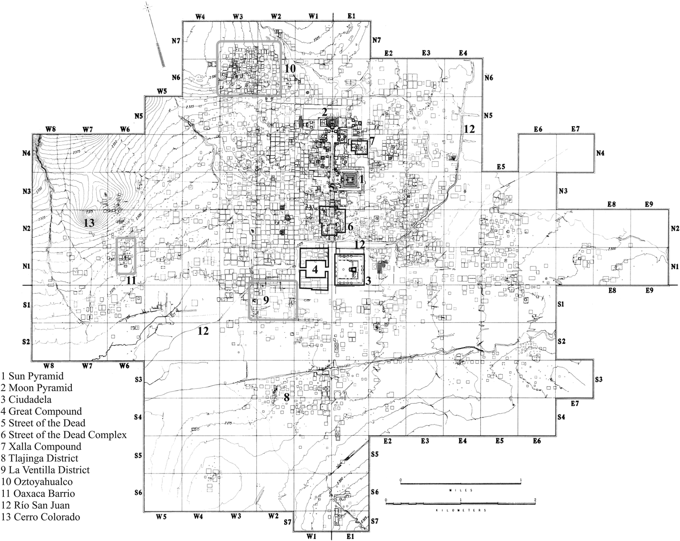
Each of the map sheets included in the Millon et al. (Reference Millon, Drewitt and Cowgill1973) publication is matched by a plastic overlay presenting architectural interpretations—simple, schematic line drawings showing outlines of buildings for which fieldworkers could see varying degrees of evidence at specific localities. These interpretations underlie the TMP map in its best-known form, a composite in which individual sheets are combined into a seamless, two-dimensional reconstruction of the architectural layout of the entire city. The result is striking: a detailed, bird's-eye view of a densely populated metropolis at the height of its size and power (Figure 1). I suspect that the cognitive maps most archaeologists have of Teotihuacan depend heavily on the rich configuration of monuments, residential buildings, and other architectural features that underlies this reconstruction. Tellingly, versions are still regularly reprinted in both specialist and non-specialist literature (for example, Cowgill Reference Cowgill2015a; Evans Reference Evans2008; Manzanilla Reference Manzanilla, Manzanilla and Chapdelaine2009), reflecting the fact that many of the most interesting issues concerning Teotihuacan are intimately tied to the spatial and organizational information that this map records and conveys.
Teotihuacan, based on the 1:40,000 scale TMP map published in Millon (Reference Millon1973:Map 1). The legend includes places referenced in the text.

But the legacy of the TMP goes well beyond its famous map. Importantly, the TMP also created a rich body of descriptive information for Teotihuacan that, around a half century later, is rivaled by few, if any, other ancient cities. These data include detailed observations about architectural and artifactual remains that were visible on the surface of Teotihuacan at the time of the survey; patterns of modern land use; and likely impacts, past and current, on the preservation and visibility of such remains. An important part of the recording process was the systematic collection of artifacts from the surface of descriptive and provenience units, materials which were brought back to the lab for analysis. Although large, numerous, and posing very significant curational challenges, the TMP artifact collections were deemed sufficiently important to preserve for future analysis. Thanks largely to the ongoing dedication of George L. Cowgill, they are still housed at a research facility managed by Arizona State University in San Juan Teotihuacan. Work on these materials continues today based on specific research interests.
Although less known than the published map, the descriptive records and artifact collections of the TMP have also played crucial roles in molding current understandings of Teotihuacan. I would argue further that the existence of these materials is an important part of what makes the map itself so valuable. The locational and architectural data captured by the TMP map are significantly more meaningful when combined with these other kinds of information—and vice versa, since the map provides the spatial information that links together the other kinds of descriptive information, making it all much more useful and intelligible.
TMP Objectives and Organization
Contributions to this special issue by Cowgill (Reference Cowgill2015b), and by Millon and Altschul (Reference Millon and Altschul2015), lay out many of the relevant details concerning the planning and organization of the TMP, subsequent analyses, and some of the key results. The aspects of the project that I emphasize here are those pertaining most directly to issues concerning the creation of surface collections, and above all the secondary data files derived from their analysis.
As noted above, a principal objective of the TMP was to map the ancient city, but this was a means to greater ends. From the beginning, it was clear to Millon and his associates that the long-term research questions that made an accurate map of Teotihuacan worthwhile and even crucial could not be addressed without collecting broader information. Activities carried out to meet these needs included: completion of field forms recording detailed descriptions of the modern terrain over which the ancient city once extended, as well as extant architectural and artifactual remains; systematic collection of stone, ceramic, and other artifacts; and strategic test excavations aimed at providing more controlled information about stratigraphy and chronology.
Preceded by shorter pilot studies, the main field phase of the TMP was initiated in 1962. Field work had largely been completed by 1966 (Millon Reference Millon1973) although some kinds of activities (especially test excavations) continued intermittently until 1978 (Altschul Reference Altschul, Whittlesey, Ciolek-Torrello and Altschul1997). The analysis of collections spanned these same periods, with most artifacts subjected to rapid, on-site tabulation, followed by more systematic analysis at the project laboratory in San Juan Teotihuacan.
A terminological issue needs to be clarified in the context of describing TMP field and lab procedures. Teotihuacan is arguably a single, large “site,” but in TMP usage the word refers to the minimum units of spatial provenience defined during the course of field observations. In much of the city, these correspond to discrete architectural features that could be observed and delineated based on surface remains. In other areas, especially in less densely population zones near the urban periphery, sites tend to be less meaningful in an emic sense, and are often defined by the borders of modern land holdings that may be significantly larger than the architectural and artifactual remains they encompass. I use the word “site” to refer to such provenience units when it is convenient, but often opting instead for the equivalent (and perhaps more appropriate) collection tract. The latter term emphasizes the fact that they define the main units for artifact collection, as well as for architectural and other kinds of descriptions.
Field Observations
Approximately 5,000 collection tracts were defined, mapped, and described by the TMP. For each tract, information about the nature and probable function of any visible architectural remains was recorded on Site Survey Record forms, along with observations about the type, quantity, and extent of construction rubble and surface artifacts. The size and height of remains were estimated where possible, along with a systematic assessment of disturbance factors (including modern land-use patterns and evidence for looting).
Collection tracts were classified according to a fairly long list of functional and architectural types. The former distinguished among residences (divided into three sub-types according to the inferred status of residents), temples, ceramic and obsidian workshops, and cemeteries, as well as various other things. Examples of the architectural types include platforms, temple bases, plazas, and several distinct forms of residential structure. Of the latter, the famous Teotihuacan apartment compound was both the most numerous and most important. Around 2,300 were recorded, and it is clear that apartment compounds housed most of the city's population after they were adopted in the Tlamimilolpa phase, after about a.d. 200.
Much more subtle was the evidence for insubstantial structures, a type of site initially identified though specific kinds of surface artifact scatters and thought likely to correspond to small, simple buildings built mostly of perishable materials. The general inference underlying the concept of the insubstantial structure—that is, that such sites may be associated with architectural remains distinct from apartment compounds—has recently been backed up in two localities by excavations exposing simple structures that appear to have housed low-status residents (Cabrera Cortés Reference Cabrera Cortés2006, Reference Cabrera Cortés2011; Robertson Reference Robertson2008, Reference Robertson2011a). More than 800 sites were assigned by TMP workers to this particular architectural type; they are therefore quite numerous, and future analyses and excavations may show that they served a range of functions beyond housing. With regard to this last point, it is worth noting that TMP records actually document this general type of site using two different architectural codes: “insubstantial structure” and “casa humilde.” The differences that these codes were intended to capture are no longer clear, and the types have mostly been lumped together in analysis. Robertson (Reference Robertson2011a) explores this and related (including demographic) issues in more detail, as well as evidence bearing on possible differences between the two codes.
Finally, and presumably at the other end of the social continuum from insubstantial structures, are “room groups,” a term used to describe heterogeneous architectural complexes concentrating around the edges of the northern part of the Street of the Dead, between the Río San Juan and the Pyramid of the Moon. The functions served by room groups are not well understood, but their association with the city's ceremonial core and the nature of artifact collections recovered from them suggest that they may often have combined elite-residential with administrative and religious purposes (Cowgill et al. Reference Cowgill, Altschul, Sload and Hietala1984:159, 181).
Surface Artifact Collections
TMP artifact collection procedures emphasized flaked stone and ceramic artifacts, although other materials (such as groundstone artifacts and samples of painted plaster) were recovered in much smaller quantities. Flaked stone samples were selected on an informal, ‘grab-bag’ basis, limiting the kinds of post-field analyses that could be usefully done with them (Michael W. Spence, personal communication; see also Andrews Reference Andrews, Hirth and Andrews2002). In contrast, rules specifying type and minimum sherd size governed the collection of ceramic materials—in general, only decorated sherds or other interpretable features such as rims, supports, and handles were taken back from the field. These rules significantly bolster the inherent comparability of ceramic collections and are a chief reason why they are useful for intrasite analyses. Of course, there are known complications, including evidence that a few fieldworkers collected unusually large quantities of specific kinds of pottery (Regular Thin Orange ware being the main example) in some specific parts of the city. Also, Aztec-period pottery may often have been collected in lower quantities than a strict application of the usual collection rules might have dictated, simply because it was encountered in such great quantities in some parts of the survey area.
TMP Computer Files
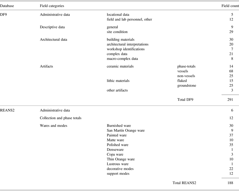
Early in the TMP research program, Cowgill began to assemble an electronic database for managing descriptive information generated in the field and laboratory. A number of versions were created; the earliest were incomplete and used mostly for testing, with later versions incorporating more data and various kinds of changes and improvements (Cowgill Reference Cowgill1993). The database designated DF8 (for “Data File 8”) was completed between about 1975 and 1977 and, in the early 1990s, converted from a mainframe VAX version into various PC-based database formats, notably Paradox (Borland International 1995). The most recent and up-to-date version of the DF lineage is DF9, a relational database built in Access (Microsoft Office 2003) by Ian Robertson. DF9 incorporates significant organizational changes over DF8 and less significant data error corrections. It contains 5,046 cases, each normally corresponding to one of the spatial collection tracts described above; information about these cases are captured by approximately 300 data fields (Table 1). Some fields provide basic administrative and locational data while others are more strictly descriptive. In addition to the kinds of information noted above about the nature of preserved architectural remains, these fields record observations about land-use and vegetative cover at the time of the survey, local effects of sediment erosion and deposition, and various other things. Roughly half of the fields capture artifact tabulations generated from typological analyses of the approximately one million artifacts comprising the TMP collections.
Summary of descriptive fields in the DF9 and REANS2 databases

A large proportion of the data contained in DF9 are ceramic tabulations based on a typology developed and put into use while TMP field surveys were still underway (Bennyhoff Reference Bennyhoff1967). Much of the initial sorting was done in the field by members of the team responsible for making the collection. Most of the potsherds were re-examined under lab conditions by a smaller number of individuals with greater expertise in ceramic analysis.
DF9 is still a crucial source of information, but its ceramic tabulations reflect the relatively limited knowledge of formal and chronological variability in Teotihuacan ceramics available when the typological criteria were first formulated in the 1960s, as well as some communication problems between the ceramic analysts and George L. Cowgill (personal communication 2001). The ceramic analysis itself, as well as other research activities running parallel to it, soon made it clear that criteria used to assign pottery to specific phases were sometimes based on mistaken ideas, while other categories failed to capture important formal distinctions. A good example of the latter is San Martín Orange, an important domestic ceramic ware captured by a single category in DF9, but known to occur as craters, amphorae, and “scraped basins”—three distinct forms made in strikingly different quantities and which probably served different functions. A number of potential categories based on combinations of formal differences (especially different bowl forms and jars) and decorative modes (various kinds of painting, polishing, and incision) were similarly excluded from the DF9 typology.
In order to generate more accurate and detailed information about the use of pottery at Teotihuacan, researchers conducted a reanalysis of all of the TMP collections using a more detailed, more refined ceramic typology. The laboratory work of the “ceramic reanalysis project” was mostly carried out in the decade between 1973 and 1983, under the general direction of Cowgill, with sorting and tabulation activities supervised by Evelyn Rattray. Project staff recorded results on specially designed, oversized paper forms, the tallies later transferred to a set of smaller coding sheets designed to facilitate computer entry. For various reasons, migrating data generated by the ceramic reanalysis into an electronic format appropriate for research purposes became a difficult and time-consuming process that suffered from numerous problems and long delays (see discussions in Robertson Reference Robertson2001). I completed a Microsoft Access database incorporating the reanalysis data (but still lacking about 300 particularly problematic cases) in the late 1990s.
The most current version of the ceramic reanalysis tabulations is designated REANS2 (Table 1). Because of some lingering incompatibilities in the definition of basic provenience units (collection tracts) for REANS2 and DF9, these databases have not been integrated into a single entity. It is nevertheless fairly straightforward to merge most cases from both databases for analyses requiring fields from REANS2 and DF9.
Future Additions
Because of continuing work with both TMP artifact collections and paper records, the corpus of descriptive information available electronically may see future additions, as well as plugging of a few important gaps. With respect to the latter, although TMP artifact tabulations do reflect the fact that large quantities of specific kinds of pottery were imported to Teotihuacan (Thin Orange and Granular ware being particularly important examples), other types of foreign pottery constitute major lacunae. For example, DF9 contains a number of fields intended to capture sherds from, or stylistically connected to, distant regions such as the Oaxaca Valley, the Gulf lowlands, and the Maya region, but only around 2,000 examples were so recorded. Rattray's work in the TMP collections reportedly identified foreign sherds at levels 5 to 10 times higher than this (Cowgill Reference Cowgill1993), suggesting that the existing records are drastically incomplete in this regard. Also, although the ceramic reanalysis forms were designed to accommodate sherds related to the three regions mentioned above, relevant counts were seldom recorded and no corresponding fields are included in derivative computer files. Given the importance of such data for addressing questions bearing on ethnicity, urban structure and identity, external economic relations, and so on, it would be extremely desirable to someday obtain and merge Rattray's tabulations with the data fields already included in DF9 and REANS2.
Digital Maps of TMP Data
In the 1990s, I digitized an electronic map of the collection tract boundaries published in Millon et al. (Reference Millon, Drewitt and Cowgill1973), the purpose of which was to facilitate geographic information system (GIS)-supported analyses and other computer based visualizations of TMP data. The first functional version of this file (designated MF2, for “Map File 2”) supplied the spatial information used in my dissertation research—involving GIS and computer-based analyses—into socio-spatial patterning at the level of Teotihuacan's neighborhoods and social districts (Robertson Reference Robertson2001). Because I digitized each of the 147 TMP map sheets separately while creating this map, MF2 incorporated large numbers of minor errors, mostly small-scale mismatches of the edges of collection tract polygons that happened to overlap margins of individual grid squares. These kinds of errors have little or no effect on many kinds of investigations, but are incompatible with analyses in which spatial relationships are assessed by the exact contiguity of tract edges and nodes. In 2009, I created a ‘topologically clean’ version of MF2 in which (along with other minor corrections) these spatial errors have been eliminated. This most recent electronic version of the TMP collection tract map is designated MF3, and versions exist in MapInfo and ESRI shapefile formats.
Other digital maps that I have created, but which I only mention in passing include a Voronoi tessellation of space around collection tract centroids derived from MF2. The polygons that compose this map are useful for spatial analyses in which it is desirable to make measurements of proximity that are unaffected by small gaps that exist at certain locations in the original TMP collection tract coverage (and as recorded in MF3). Also, I have begun digitizing the architectural interpretation sheets published in Millon et al. (Reference Millon, Drewitt and Cowgill1973); when completed, this map will probably be most useful for displaying or visualizing results actually generated by analyses based on MF3 or its Voronoi equivalent.
EXAMPLES OF TMP-BASED STUDIES
Since space does not permit me to review many of the important studies that have made use of TMP surface data, I focus on a few examples that illustrate different approaches and problems. Although I also concentrate on analyses that make use of spatial information, I begin by briefly characterizing an early line of analysis that was essentially nonspatial, but which has been influential in how we think about Teotihuacan in demographic terms.
Nonspatial Approaches: Demographic Estimates
The work in question involved combining TMP architectural and artifactual data in order to make diachronic estimates of the urban population of Teotihuacan. At the foundation was René Millon's estimate of the numbers of individuals housed by Xolalpan phase (a.d. 350–500) apartment compounds. Millon began by calculating the amount of sleeping space afforded by a number of variously sized apartment compounds whose plans were known through excavation. He then extrapolated these figures to the more than 2,000 apartment compounds occupied during the Xolalpan phase, and which, while almost all unexcavated, had been characterized in terms of size by the TMP. Millon arrived at figures suggesting a population of 125,000 individuals, with 75,000 a more conservative, if less probable minimum (Millon Reference Millon1973:44–45, see also Millon Reference Millon1970). Later, Millon revised his assumptions to favor a Xolalpan phase population between 150,000 and 200,000 individuals (Millon Reference Millon and Hammond1974:354–355).
Millon's estimates were of Teotihuacan's population at the height of the city's size and power. The lack of comparably detailed architectural records for other phases precluded using the same approach for earlier and later periods, but Cowgill (Reference Cowgill and Hammond1974) built on Millon's analysis by using the ratio of Xolalpan population figures to the total count of Xolalpan sherds as a basis for converting sherd counts for other phases (taking into account variation in their lengths) into population estimates.
Important insights emerging from Cowgill's work were that Teotihuacan grew very rapidly early in its history (during the Patlachique phase [150–1 b.c.]) while later rates of growth (particularly after the end of the subsequent Tzacualli phase [a.d. 1–150]) were much slower. Since sherd densities revealed little evidence for a significant decrease in occupation intensity during the Metepec phase (a.d. 500–600), Teotihuacan's demographic profile may have been characterized by a long plateau, stretching from approximately a.d. 150–550 (Cowgill Reference Cowgill and Hammond1974:377–395).
A detailed consideration of what the tabulations generated by the TMP ceramic reanalysis project imply for Teotihuacan population issues is something I will present in a separate publication, but it is worth noting here that sherd totals for various occupation phases in REANS2 suggest some modifications to the demographic profile described by Cowgill on the basis of earlier analyses. Taken essentially at face value (but accounting for probable differences in phase length), REANS2 phase totals show no evidence for a post-Tzacualli demographic plateau, but instead reflect relatively steady rates of average increase connecting an initial Patlachique growth spurt to a prominent peak in the Xolalpan phase. In contrast, total Metepec counts imply a marked decrease in average population after the Xolalpan phase. Density maps indicate that population loss may have been most pronounced in the city's peripheral zones, although the intensity of occupation in residential areas surrounding the ceremonial core also appears to be diminished compared to Xolalpan.
As Cowgill (Reference Cowgill and Hammond1974:370–373) has cogently discussed, important assumptions underlie both his interpretations and mine, including ideas about the per-capita production and consumption of potsherds, the relative duration of phases, and the surface visibility of sherds from different occupation periods. Unfortunately, all of these issues remain seriously underexamined. A separate issue concerns the veracity of the ceramic typology underlying REANS2—above all, its ability to reliably assign fragmented pottery to the various ceramic phases and subphases currently recognized at Teotihuacan. Briefly, although I would argue that our knowledge of ceramic change at Teotihuacan is still in need of considerable refinement, I also feel that the ceramic reanalysis does (as was intended) represent an important improvement over the DF9 ceramic data in most respects. I note in passing that, as part of my dissertation studies (Robertson Reference Robertson2001), I carried out a long series of statistical tests designed to red-flag ceramic types from the reanalysis that may have problematic affiliations with the phases in which they are supposed to have been used. This work (mostly based on boot-strapped estimates of correlation between individual ceramic type counts and phase totals) revealed only a few clear chronological issues, and none of a type likely to affect the rather general, REANS2-based, conclusions presented above.
Early Artifact Distribution Maps
Among the earliest spatial visualizations of TMP artifact tabulations were maps using contours to show smoothed variation in the distribution of specific artifact types—with raw counts either standardized as densities, or within larger pools of artifacts as proportions. Cowgill created and published a number of these, starting with maps showing sherd densities for specific occupation phases (Cowgill Reference Cowgill and Hammond1974), with later examples based on densities and proportions of specific artifact types, above all major types of pottery (Cowgill Reference Cowgill, de Tapia and Rattray1987; Cowgill et al. Reference Cowgill, Altschul, Sload and Hietala1984). Their production was relatively laborious, involving custom computer programs that generated summary data at the nodes of a regularly spaced grid (usually 250 × 250 m), followed by hand drafting of contours. They were nevertheless highly productive tools for answering basic questions and raising new ones—especially about the diachronic trends in urban growth and internal patterns in artifact consumption.
Examples of contour maps that have been of particular interest to other researchers concern San Martín Orange ware (SMO) pottery. Most SMO was produced in Xolalpan- and Metepec-phase workshops in the Tlajinga district (Sheehy Reference Sheehy1992; Sullivan Reference Sullivan2006), a part of the city where Cowgill's maps (Cowgill et al. Reference Cowgill, Altschul, Sload and Hietala1984: Figure 5, Reference Cowgill, de Tapia and Rattray1987: Figures 2 and 3) show notably high densities and proportions of the ware. Linda Manzanilla (Reference Manzanilla and Berlo1992, Reference Manzanilla and Manzanilla1997) has drawn attention to an area well outside the Tlajinga production district where Cowgill also noted high proportions of SMO—a large zone roughly parallel to, and some 300 m west of, the northern part of the Street of the Dead (Figure 1). Manzanilla cited the existence of this area in support of an economic model involving food, centralized storage and redistribution, and the Teotihuacan priesthood. The merits of the particular argument aside (see Millon [Reference Millon and Berlo1992:376–382] for a critique), this is an opportunity to correct an error made by Manzanilla in tying this zone to high levels of SMO amphorae consumption. In fact, Cowgill's maps and discussion were based on analyses that (as discussed above) did not yet distinguish among the several vessel forms that were made of this ware. As I show below, these types exhibit distinct distributional patterns and amphorae show only a modest connection to the zone in question.
Later-Generation Statistical Maps
Contour maps of the type discussed above remain extremely important for identifying and describing relatively broad spatial patterns and trends—that is, of a scale large enough to not be eradicated by the smoothing effects that underlie the mapping procedures. Fortunately, the labor in making them has been drastically reduced by the availability of modern statistical computing software such as R, and GIS and mapping software such as ArcGIS and Surfer.
Similar advances in software make it straightforward to shade or color a lattice-based map such as MF3 to show spatial variation at the level of individual collection tracts. Choropleth maps complement contour maps and are most useful for examining small-scale spatial variation—differences in artifact composition, for example, which might distinguish nearby or even adjacent tracts. Such maps, however, are also prone to conveying high levels of noise due to sampling error, an effect that can seriously compromise recognition of underlying patterns (Kennedy Reference Kennedy, Goodchild and Gopal1989). Bayesian estimation methods (particularly empirical approaches that combine locally based prior estimates with individual sample data) have been particularly helpful in dampening such effects in exploratory map analysis, and also as a means of pre-treating data for more formal statistical evaluation. I have elsewhere discussed such an approach, contrasting a thematic map of observed SMO ware proportions with one based on posterior point estimates from an empirical Bayesian filter (Robertson Reference Robertson1999). The latter shows greater clarity and interpretability in various respects, notably including a sharp and highly localized drop in SMO proportions centered on a pair of temple complexes in Oztoyahualco, a district near the northwestern periphery of the city distinguished by its large numbers of relatively small and closely packed apartment compounds (Figure 1). Extended applications of the Bayesian procedure and some methodological enhancements are discussed in Robertson (Reference Robertson2001).
Methods for spatial-statistical analysis have continued to develop rapidly in recent years. A new approach proving useful in tandem with Bayesian methods stems from the concept of local indicators of spatial association (LISA). As implemented in the software packages GeoDa (Anselin et al. Reference Anselin, Syabri and Kho2006) and R (R Development Core Team 2010), LISA provides coefficients and graphic tools for examining local variation in spatial autocorrelation.
Before I briefly consider an example based on TMP data, a few nontechnical details need to be laid out. First, LISA coefficients such as Local Moran's I measure the degree to which values exhibited by individual cases correlate with those found in larger groups of nearby cases (Anselin Reference Anselin1995); essentially, they provide location-specific measures of spatial association that have the potential to reveal different forms of spatial clustering. The significance of Local Moran's I can be assessed using spatial randomization procedures (Lloyd Reference Lloyd2011:89), and cases determined to be of further interest interpreted with respect to a Moran scatterplot (Anselin Reference Anselin, Fischer, Scholten and Unwin1996). The latter classifies significant cases according to four categories, depending on whether they exhibit low or high values (that is, above or below the mean for all cases) and whether the pattern of association with neighboring cases is positive or negative. The former include high-high cases, meaning they exhibit high values in neighborhoods that also, collectively, exhibit high values—in other words, a spatial cluster of cases with values above the global mean. Low-low cases indicate the opposite kinds of clusters. Negative association is represented by high-low and low-high cases; in these last types, clusters are formed by cases embedded in larger neighborhoods exhibiting contrasting values.
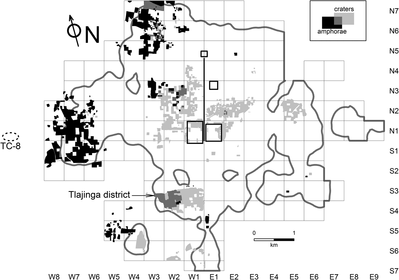
Returning to Teotihuacan, Figure 2 contrasts the distribution of LISA-derived high-high clusters for SMO craters and amphorae, two of the three forms of SMO captured by the ceramic reanalysis project. The data underlying these results are empirical Bayesian estimates of proportions, calculated within a pool of total Xolalpan and Metepec phase sherd counts for individual collection tracts. R and GeoDa were used to prepare a spatial weights matrix listing the eight nearest neighbors of all individual cases, and then subsequently to 1) identify those with significant (here, meaning p ≤ .05) Local Moran's I values, and 2) classify them according to the four association types described above. In Figure 2, high-high cases from the amphorae analysis are plotted in black, while those from the crater analysis are in light gray; the few locations of overlap (where cases are high-high for both ceramic types) are plotted in an intermediate shade of gray. (To simplify discussion and because of the difficulty of distinguishing larger numbers of classes without color-coding, no other association types are included in this figure. For similar reasons, I have also omitted locations of high-high cases for scraped basins, the third major vessel form made in SMO. I briefly comment on the distribution of scraped basins below.)
LISA cluster plots showing cases classified as ‘high-high’ for posterior estimates of San Martín Orange crater and amphora proportions. For reference, an approximate outer boundary for the city is indicated by a gray line, based on a contour associated with a Xolalpan phase sherd density of 5 sherds/hectare/century (Robertson Reference Robertson, Gorenflo and Sanders2007). The location and size of site TC-8 reflect my best understanding of information in Sanders et al. (Reference Sanders, Parsons and Santley1979), Sanders (Reference Sanders1994), and Gorenflo and Sanders (Reference Gorenflo and Sanders2007), but should be regarded as approximate.

Two general but important points emerge from Figure 2. First, for both SMO types under consideration, high positive association produces relatively large spatial clusters concentrating in significant parts of the city. Second, these areas of concentration are largely distinct, with only one really notable example of overlap. At the most basic level, these observations implicate the two vessel types in socioeconomic behaviors that are strongly structured spatially, but also quite distinct in terms of specific locations.
As one might predict, the main area where the two kinds of high-high clusters do overlap is Tlajinga, the district where most SMO was made. Interestingly, however, high-high cases emerging from the crater analysis cover almost the entire district, while those related to amphorae are confined to the western half. This may reflect a level of internal specialization within the larger potting community, with relatively higher levels of amphorae produced in workshops situated in its western half. This possibility accords well with Sullivan's (Reference Sullivan2006) detailed reanalyses of TMP collections from Tlajinga. Although wasters and other empirical measures of production intensity suggest that most workshops usually made more than one of the major SMO vessel types, her indicators for amphorae production were expressed most strongly in collections from the western half of the district.
Outside of Tlajinga, most of the high-high cases for crater proportions concentrate in largely residential districts near to the city core. The largest block is situated to the west of the Street of the Dead, overlapping the northern platform of the Great Compound and running some distance to the north and northwest—essentially across the zone that Cowgill (Reference Cowgill, de Tapia and Rattray1987) and Manzanilla (Reference Manzanilla and Berlo1992, Reference Manzanilla and Manzanilla1997) drew attention to in their respective work (see above). Another large cluster is located on the other side of the ceremonial core, north and northeast of the Ciudadela and flanking the north bank of the Río San Juan. It is reasonable to hypothesize that these two areas were largely dominated by households making relatively high demands on SMO craters in their food storage and cooking activities. Different analyses discussed in Cowgill et al. (Reference Cowgill, Altschul, Sload and Hietala1984) associate high SMO proportions with high and (perhaps less clearly) intermediate status apartment compounds; these interpretations of status could reasonably and tentatively be extended to these zones of high-high clustering presented here, at least for the phases in question (Xolalpan and Metepec).
In marked contrast to craters, most high-high amphorae locations concentrate in two major zones on the western periphery of Teotihuacan. The first and largest of these lies several kilometers due west of the city's geographic center—on the southern flanks of a hill called Cerro Colorado and immediately west of the ethnic enclave known as the “Oaxaca Barrio” or Tlailotlacan (Spence Reference Spence and Berlo1992). A less cohesive area of concentration is associated with Oztoyahualco, in the northwest part of the city. Most cases fall on the outskirts of the district, but some cases lie directly within it.
The spatial association of high-high SMO amphorae cases and the area south of Cerro Colorado (and perhaps the western periphery of Teotihuacan in general) is intriguing. In this area, apartment compounds are relatively low in number and density, while collection tracts recorded as insubstantial structures are quite common. Compared to districts closer to the city core, this zone appears to have preserved relatively large amounts of open space that may have offered some potential for urban gardening and cultivation (Robertson Reference Robertson2008). Amphora-shaped ceramic vessels have been tied to the exploitation of maguey sap in various ethnographic and archaeological contexts in central Mexico (Bey Reference Bey, George, Pool and Bey2007; Fournier García Reference Fournier García2007; Parsons and Parsons Reference Parsons and Parsons1990; Sheehy Reference Sheehy and Drooker2001), and one tantalizing possibility is that the association of high-high SMO amphorae clusters with a sparsely settled urban zone reflects their use in the production and subsequent transport of aguamiel and pulque. Maguey plants can be grown almost anywhere in the Teotihuacan Valley, but they are particularly suited to the rising piedmont terrain on the western and northwestern edges of the city, where, at least in recent times, soil and water conditions have favored maguey cultivation.
Potentially strengthening the connection between Teotihuacan's western periphery and a possible role in maguey cultivation is a settlement recorded by the Teotihuacan Valley Survey a short distance outside the TMP survey grid, only a kilometer or so to the west (Figure 2) (Gorenflo and Sanders Reference Gorenflo and Sanders2007: Figure 4.17). Site TC-8 (also known as Maquixco Bajo) has been interpreted as a large village of 500–600 inhabitants. The recovery of unusually large numbers of obsidian tools shaped for scraping maguey plants as part of the process of sap recovery led Sanders and his colleagues (Sanders Reference Sanders1994:63; Sanders et al. Reference Sanders, Parsons and Santley1979:347) to suggest that aguamiel and pulque played a key role in the community's economy. Some of the families living at TC-8 likely did farm and process maguey plants themselves. The approximately 300 scrapers recovered there, however, came from residential contexts and were not associated with any evidence for local manufacture; conceivably, they may have been stockpiled for trade to farmers who actually made use of the tools in fields located further east, in the vicinity of Cerro Colorado. It is also possible (but more speculative) that TC-8 may have functioned as a kind of depot, where maguey sap was exchanged for scrapers, foodstuffs, and other products, before being transported to markets within Teotihuacan. A similar role for the settlement, but involving a more exotic product, has been suggested by Widmer (Reference Widmer, Mastache, Parsons, Santley and Serra Puche1996), who sees TC-8 as a node in the transport of Pacific marine shell into the same urban markets.
The previous discussion of the LISA-based map shown in Figure 2 was deliberately exploratory in tone, aimed at highlighting how maps that summarize robust distributional properties can raise productive questions and hypotheses. But they can also feed into more formal kinds of analyses. Before moving to the next section of the paper, I use correspondence analysis (CA) to examine how sites classified as high for the various SMO varieties relate to the various kinds of architectural features identified at the same localities. In this, I go beyond what was illustrated in Figure 2 by considering both positive and negative association (that is, high-high and high-low cases) and also by bringing in information pertaining to the distribution of San Martín Orange scraped basins—as with craters and amphorae, assessed as Bayesian posterior estimates of proportions within a pool of Xolalpan- and Metepec-phase sherd totals. It may be helpful to note that this third form of SMO is far less common than either of the other two, and appears to have been used at higher levels in the Metepec than the preceding Xolalpan phase. As far as spatial distribution goes, high-high clusters for scraped basin proportions are both less numerous and less dispersed than for the two types illustrated in Figure 2. Apart from expected concentrations in the SMO-producing Tlajinga district perhaps the most striking clusters of high-high cases are associated with specific areas in or around the Ceremonial Core—notably including the Street of the Dead Complex, as well as parts of residential zones immediately to the east and southeast of the Xalla Compound, and parts of the Xalla Compound itself.
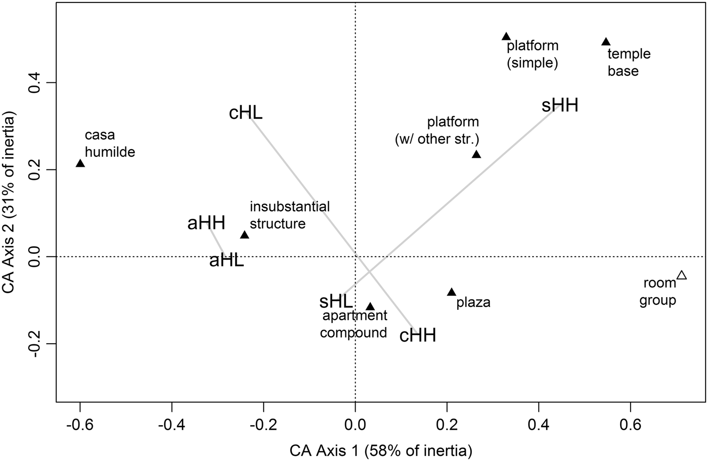
The main architectural types represented among the roughly 1,300 cases identified as either high-high or high-low for one of the three SMO vessel forms are temple bases, two kinds of platform (“simple” and “platforms supporting other structures”), room groups, plazas, apartment compounds, and the two kinds of ephemeral structure mentioned previously: insubstantial structures and casas humildes. These architectural types were cross-tabulated against the two LISA-based association types; this was done separately for each of the SMO forms, and the three tables combined into a single (stacked) table for correspondence analysis. The goal of the CA was to obtain a low-dimension summary of the main relationships between the rows and columns of the stacked table—that is, architectural types and the association types distilled from the spatial distribution of San Martín Orange pottery. Such a summary is presented in Figure 3. Here, scores for both dimensions of the stacked table are superimposed on the first two CA axes, which together account for almost 90% of the inertia in the original table (see Greenacre [Reference Greenacre2007] and Clausen [Reference Clausen1998] for technical aspects of correspondence analysis).
The first two axes of a correspondence analysis (CA) of a ‘stacked’ cross tabulation of architectural types and ‘high’ positive and negative spatial association clusters for all three forms of San Martín Orange ware. The lowercase prefix for the association types designates the form (c = crater, a = amphora, s = scraped basin). The uppercase suffix indicates the type of positive association (HH = ‘high-high,’ HL = ‘high-low’). Note that ‘room group’ (plotted with an open triangle) is a ‘supplementary point’ in this analysis, meaning that for technical reasons corresponding counts in the underlying table were prevented from playing a role in defining the CA axes.

A full explication of this plot goes beyond the scope of this paper, but a few of the more salient relationships deserve comment. Notably, temple bases and both types of platforms fall into the same part of the space defined by the two CA axes as the high-high type for scraped basins (labelled sHH in Figure 3). In short, this suggests that these types of structures are more likely than others to contribute to spatial clusters of collection tracks characterized by high proportions of SMO scraped basins. Although the reasons for this are probably complex, it is significant that these three architectural types are broadly and collectively suggestive of civic-ceremonial activities; conceivably this particular form of SMO vessel (at least sometimes featuring curvilinear and floral designs in red paint [for example, Rattray Reference Rattray2001:Figure 192]) may have been used in ritual activities that were preferentially carried out in such contexts, likely involving at least some individuals that we would identify as “elites.”
The proximity of the two types of insubstantial structure and both the high-high and high-low LISA-types for SMO amphorae suggests something quite different—specifically, the prevalent use of amphorae in parts of the city where insubstantial structures (and, by implication, the activities of nonelites) predominated. This reinforces previous discussions highlighting the presence of high-high amphorae clusters in the western periphery of Teotihuacan and implications for possible maguey sap production. One new observation emerging from the CA work is that both high-high and high-low cluster types for amphorae show similar associational patterns with respect to architectural types (that is, aHH and aHL fall in the same parts of the plot). This stands in contrast to LISA clusters for the other two types of SMO, where the high-high and high-low (HH and HL) association types fall into very different parts of the CA space; clearly, the kinds of architectural types implicated in clusters involving high proportions of SMO craters and scraped basins vary depending on whether or not surrounding collection tracts show similarly high, or contrastingly low, proportions. For example, when high proportions of scraped basins are recovered from apartment compounds, they tend to be embedded in neighborhoods where proportions of such sherds are relatively low—so, constituting a kind of local outlier. On the other hand, and as noted previously, positive clusters involving scraped basins tend to be associated with architectural types that were probably used for nonresidential activities that typically involved high-status agents. Again, a more in-depth discussion of the behavioral implications of this observation goes beyond the goal of this paper. My purpose here is simply to illustrate how combining exploratory with more formal analyses of the right (that is, detailed and spatially extensive) kinds of data can begin to illuminate contrasts that are fundamental to the socio-spatial texture of a complex city.
Multivariate Approaches: Socio-Spatial Variation, Barrios, and Urban Boundaries
Univariate visualizations involving single artifact types remain important tools for working with TMP data, but there are limits to the kinds of questions they can address. More complex urban phenomena, such as material expressions of status differences and the nature of internal socio-spatial divisions, are more likely to be illuminated by analyses involving broader ranges of material culture. Early attempts to tackle problems of these kinds using multivariate analyses of TMP surface data include investigations by Sload (Reference Sload1982, Reference Sload, de Tapia and Rattray1987) into status variation, and by Altschul (Reference Altschul1981, Reference Altschul, de Tapia and Rattray1987, Reference Altschul1993) into barrios, both parts of more broadly conceived dissertation studies. I concentrate here on Altschul's work because it provides more relevant background for a brief characterization of some of my own work, to be considered shortly.
Barrios
Much of what has been said about the internal organization of Teotihuacan has revolved around the barrio—an imprecise concept that has been used there (as elsewhere in Mesoamerican ethnography and archaeology) to refer to a range of spatial entities that were likely quite different socially (Mulhare Reference Mulhare1996:99–100; Smith and Novic Reference Smith, Novic, Arnauld, Manzanilla and Smith2012:14–15). There were various reasons for this focus. One motivation for investigating barrios at Teotihuacan arose from early versions of the TMP map and the first analyses of related collections. The map revealed that, in some areas, groups of apartment compounds form spatial clusters and/or reflect levels of architectural coordination that make them appear distinct relative to surrounding areas (Cowgill Reference Cowgill and Stone2007:279; Millon Reference Millon and Sabloff1981:210–212). Architectural groupings of this type were naturally compared to neighborhood-level spatial entities often described as barrios in historic and contemporary settlements. While underlying social meanings could not be determined simply on the basis of size and shape, lab analyses revealing spatial concentrations of other materials in other parts of the city (particularly foreign potsherds and evidence for lithic and ceramic workshops [Krotser and Rattray Reference Krotser and Rattray1980; Rattray Reference Rattray, de Tapia and Rattray1987; Spence Reference Spence and Isaac1986]) suggested that barrio-like structures in Teotihuacan may sometimes have been organized around ethnic and occupational differences.
At a more theoretical level, an interest in barrios was driven by recognition that spatial entities intermediate in scale between cities and the fundamental architectural and social units of which they are comprised are crucial for understanding urban dynamics. They have important structuring effects on socioeconomic networks involving cooperation, reciprocity, resistance and exploitation, and they may largely arise from such networks. Less organically, they may also be imposed in whole or in part by central authorities, perhaps to fulfill administrative functions (Robertson Reference Robertson2001, Reference Robertson, Gallut and Peralta2011b; Smith Reference Smith2010).
Millon (Reference Millon and Sabloff1981:211) made a map of approximately 150 possible barrios in Teotihuacan, based largely on spatial arrangements of structures, but sometimes taking into account evidence for workshop clusters and patterned variation in the distribution of artifacts. This was preliminary work that was never published, but it set the stage for Altschul's (Reference Altschul1981, Reference Altschul, de Tapia and Rattray1987, Reference Altschul1993; see also Cowgill et al. Reference Cowgill, Altschul, Sload and Hietala1984) more formal investigations of barrio-like spatial structures using TMP surface data. His approach was essentially exploratory: to determine whether or not spatially patterned variation in the composition of ceramic artifact collections might reveal entities similar in scale and form to ethnographically documented barrios. Altschul focused his work on identifying “internally homogenous” barrios, envisioned as sets of collection tracts that (1) exhibit levels of internal variation that are low relative to other sets of tracts, and (2) form contiguous spatial groups. Acknowledging that other kinds of spatial entities likely existed at Teotihuacan, Altschul felt that homogenous barrios were most likely to be identified using surface artifact collections (Cowgill et al. Reference Cowgill, Altschul, Sload and Hietala1984:182).
The procedure used to search for barrios involved hierarchical cluster analysis using collection tracts as cases, with tabulations of 16 DF8 ceramic types attributed to the Xolalpan and Metepec phases used as variables. Due to limitations inherent in available computer hardware and software, parallel analyses were carried out on subsets of collection tracts located in three different parts of the city. Altschul (Reference Altschul, de Tapia and Rattray1987, Reference Altschul1993) described his attempts to identify spatial entities that could be plausibly interpreted as barrios as having only mixed success. Perhaps the clearest example of a possible identification of a barrio came from an area just west of the Great Compound. Here, 21 cases identified by cluster analysis as sharing similar ceramic profiles also formed a relatively clear group of contiguous structures in the northwest corner of square N1W2. This is an area that coincides relatively closely with one in which Spence's revised assessments of TMP lithic data suggest a number of probable obsidian workshops (Spence Reference Spence1981, and personal communication 1998), and it is possible that part of what made the 21 cases appear distinctive in terms of discarded ceramic materials were shared behaviors and identities related to a barrio-level involvement in obsidian tool production. For the most part, however, Altschul's work generated clusters lacking the level of spatial coherence anticipated for possible barrios.
Neighborhood variation and social districts
A factor complicating Altschul's work was the explicit focus on identifying barrios in which internal variation was assumed to be minor relative to external variation. More recently, and making use of newly available ceramic reanalysis data, I have carried out investigations designed to identify spatial entities configured in potentially more complex ways and not necessarily internally homogeneous (Robertson Reference Robertson2001, Reference Robertson, Gallut and Peralta2011b).
In short, the approach consisted of a two-stage, nested classification of collection tracts. In the first stage, tracts representing a range of different kinds of structures (but including apartment compounds, insubstantial structures, and room groups) were classified on the basis of ceramic artifacts collected from their individual surfaces. This part of the procedure was conceptually similar to Altschul's work, and cluster analysis (although a nonhierarchical form) was the method employed. The second stage of classification addressed a higher scale of resolution; individual collection tracts were classified again, but on the basis of neighborhood-level differences, specifically a characterization of the mixture of first-stage classes found within a relatively short distance of one another. This was assessed by tabulating first-stage classifications within buffers that extended the perimeters of each of the collection tracts outward by a distance of 130 m. These tabulations were then used as input variables for a second cluster analysis.
The first classification provided a crude ordinal scale measuring the wealth and status of pottery-consuming residential groups. The second classification stage indicated how such groups, characterized in terms of wealth and status, combined into analytical neighborhoods of roughly similar sizes. Did households of comparable status levels co-associate to form relatively homogeneous barrios, similar to the kinds of spatial structures sought by Altschul? Or did they intermingle, forming some sort of social mosaic? If the latter, were different kinds of social mosaics associated with different parts of Teotihuacan?
Because it is possible to separate most pottery according to occupation period, these kinds of questions can be approached diachronically. In the remainder of the discussion I contrast results for the Miccaotli phase (approximately a.d. 150–200, the period of occupation immediately before the adoption of apartment compounds at Teotihuacan) and the Tlamimilolpa phase (approximately a.d. 200–350, the period in which apartment compounds were broadly adopted across Teotihuacan).
The reanalysis ceramic categories that underlay these analyses encompass vessel forms used in various activities and contexts, ranging from everyday cooking and storage to somewhat less mundane contexts of food service. Some types were probably more important in socially charged activities such as feasting, others in the performance of sacred rituals. Tabulations describing relative quantities of relevant sherds were standardized as proportions within phase-specific pools, and then pretreated using empirical Bayesian methods to dampen effects of sampling error. I confine remaining discussion to solutions in which four clusters were defined for each of the two phases included in the analysis.
Summary: Wealth/status variation
In many respects (and, above all, with regard to the first-stage classification) the results were similar for both phases. Patterns of association among ceramic categories used as input data indicate that the defined classes reflect differences in the general household activities alluded to just above (food storage and preparation, service, and ritual) emphasized at localities sampled by collection tracts. Various lines of evidence—but in particular variation in the degree of energy invested in the manufacture of different vessel types, inferred use, and above all, patterns of association among types of pottery—suggest that cluster memberships measure broad differences in the wealth and status of individuals and households whose activities generated the discarded pottery. For convenience, the four clusters can be regarded as signatures of high, low, and two levels of intermediate status. Although distinctions between the different clusters cannot be fully considered here, it is worth noting that collections interpreted as high status tend to be characterized by high proportions of well-finished, decorated vessels in forms used for serving cooked food; domestic cooking and storage wares are present, but in modest amounts. At the other end of the spectrum, collections interpreted as low status exhibit much lower diversity in terms of the representation of ceramic types and tend to be dominated above all by the largely undecorated cooking and storage pot known as the olla. The most important distinction between the two classes characterized as intermediate in status is that one exhibits notably high proportions of cooking and storage vessels; moreover, spatial-statistical assessments that I do not describe here show that this same class shares a high degree of spatial association with collection tracts interpreted as high status, at least in many districts. I have argued that many of the cases assigned to this particular form of intermediate class were likely connected through some kind of “patron-client” relationship with high-status households, and that they may (among other things) have provisioned such households with cooked food (Robertson Reference Robertson2001, Reference Robertson, Gallut and Peralta2011b). (Note that in the context of this discussion, I use the word “class” to refer strictly to units created by a process of classification, in this case cluster analysis. Although they have socioeconomic meaning, I do not mean to imply that they necessarily reflect well-defined or well-bounded social classes in Teotihuacan society.)
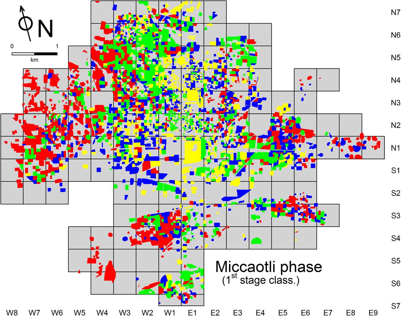
Figure 4 shows the distribution of classes defined by the first stage cluster work for the Miccaotli phase. The four classes are to varying degrees dispersed over the city, intermingling in many areas to form complex mixtures. The lack of any strict segregation of classes defined at this stage means that most parts of the Miccaotli phase city were relatively diverse in socioeconomic terms, many neighborhoods and even adjacent collection tracts exhibiting striking contrasts in inferred wealth/status levels.
Map showing first-stage classification for the Miccaotli phase. (Colors code wealth/status classes as follows: yellow = high; red = low; green and blue = intermediate; blue specifically indicates intermediate cases characterized by high proportions of cooking and storage vessels, and high spatial association with high status cases, while green indicates all other intermediate cases.)

But these classes are not randomly distributed. In fact, in spite of the expressions of localized social diversity described above, they simultaneously exhibit a clear tendency for self-association. Although at least some examples can be found in most parts of the city, each class tends to occur in higher concentrations in some parts of the city than in others. For example, the class interpreted as a signature of activities of wealthy and high-status individuals (colored yellow in Figure 4) is most common in the vicinity of the city's civic-ceremonial core, along the sides of the Street of the Dead. Households from the opposite end of the socioeconomic spectrum (in red) tend to concentrate near the periphery of Teotihuacan. The intermediate wealth/status levels (blue and green) were most common in parts of the city that were also spatially intermediate, relative to areas dominated by households occupying the two poles of a wealth/status dimension. (Note that blue is used in Figure 4 to indicate the specific kind of intermediate status class interpreted as sharing a spatial and behavioral relationship with high-status households.)
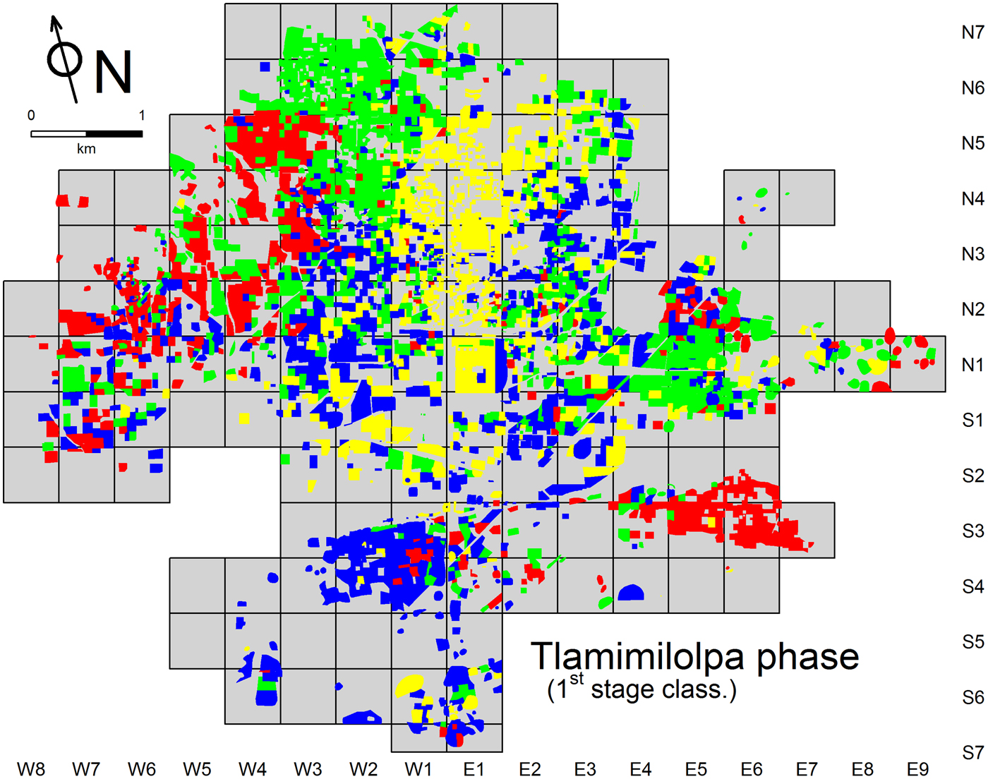
Many of the observations that have been made about the nature and distribution of first-stage classes for the Miccaotli phase apply in general terms to the subsequent phase. Notably, the classes defined for the Tlamimilolpa phase (Figure 5) are also relatively dispersed and intermingled, and also form similar patterns of spatial concentration. As was the case for Miccaotli, for example, collections associated with individuals from the upper-end of the wealth/status continuum were most common around the civic-ceremonial core, while areas of concentration exhibited by the other Tlamimilolpa classes parallel those already noted for the preceding phase.
Map showing first-stage classification for the Tlamimilolpa phase. (See caption for Figure 4 for details on color-coding.)

The main contrast between the two phases has to do with the degree of self-association exhibited by the first-stage classes—during the Tlamimilolpa phase, the tendency for each of the classes to concentrate in specific parts of the city is much stronger than it was during the Miccaotli phase, signaling a significant reduction in the diversity of Teotihuacan's neighborhoods. While this is relatively clear in a visual comparison of Figures 4 and 5, evidence presented in the discussion of the neighborhood-based analysis (below), strengthens the claim in quantitative terms.
Summary: Neighborhood-level classification and social districts
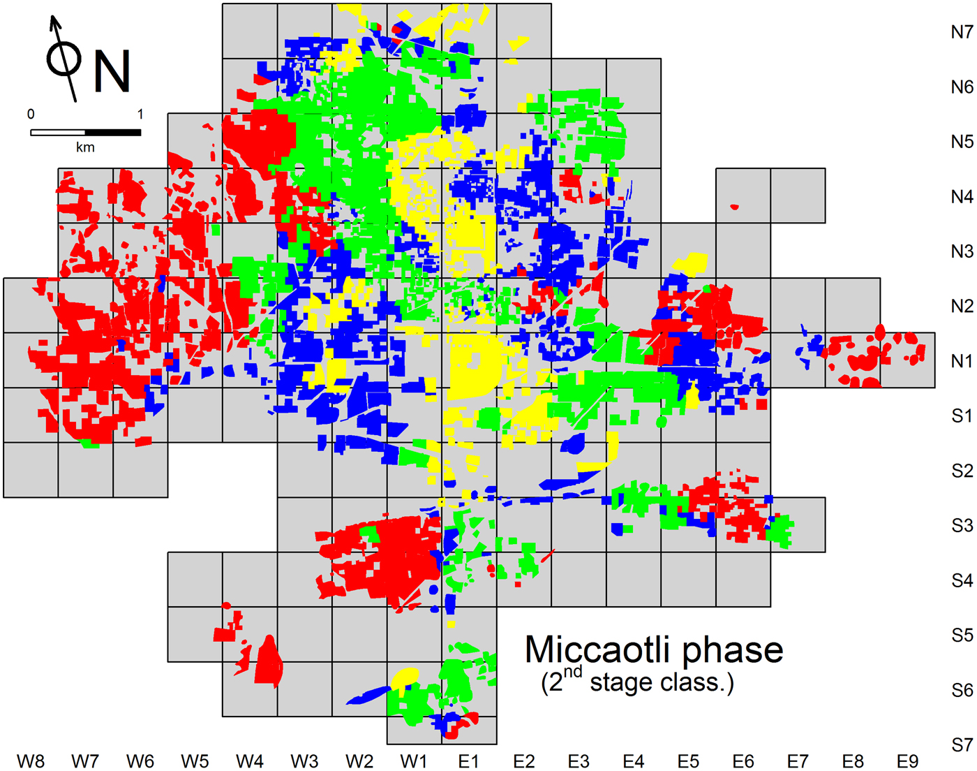
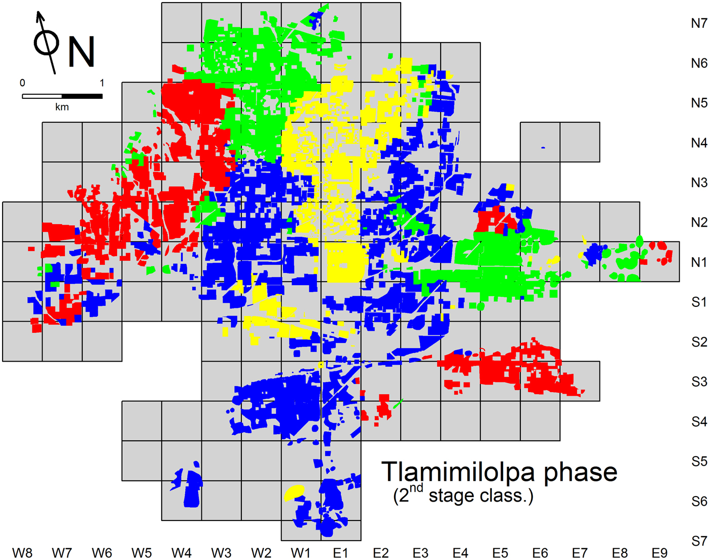
The second stage of classification steps back from the fine-grained detail inherent in the structure-by-structure maps described above to reveal broader patterns. In marked contrast to the pervasive intermingling of first-stage classes, the distribution of the four classes defined at this stage in the analysis, and specifically their high degree of spatial self-association, divides Teotihuacan into relatively well-defined subregions, each containing neighborhoods that exhibit similar mixtures of wealth and status levels. An appropriate term for describing the internal divisions that emerge from this is social district. Evident for the Miccaotli phase (Figure 6), the effect is particularly clear for the Tlamimilolpa phase (Figure 7). In fact, one of the important insights to emerge from a comparison of the two phases is the degree to which the urban landscape had, by Tlamimilolpa times, become organized into a smaller number of larger, better delimited and more coherent social districts.
Map showing second-stage (neighborhood-level) classification for the Miccaotli phase.

Map showing second-stage (neighborhood-level) classification for the Tlamimilolpa phase.

This tendency is most obvious in the geographic and symbolic core of the city, the civic-ceremonial zone around the Street of the Dead. While there is a clear spatial association between this part of the city and one of the neighborhood-level (second stage) clusters defined for the Miccaotli phase (Figure 6), the corresponding social district is divided into two sections, separated by a clear gap of several hundred meters—in the vicinity of the Street of the Dead Complex, a short distance north of the Río San Juan. Compared to the Miccaotli phase, the social district associated with the Street of the Dead area during the Tlamimilolpa occupation (Figure 7) had coalesced into a single unit, one exhibiting greater spatial cohesion, and likely tighter social integration as well. Much of the boundary delimiting this zone maps onto architectural discontinuities clearly visible in architectural interpretations of the TMP map (some of which can be glimpsed in Figure 1), and the gap that existed in the Miccaotli phase no longer exists in the Tlamimilolpa phase.
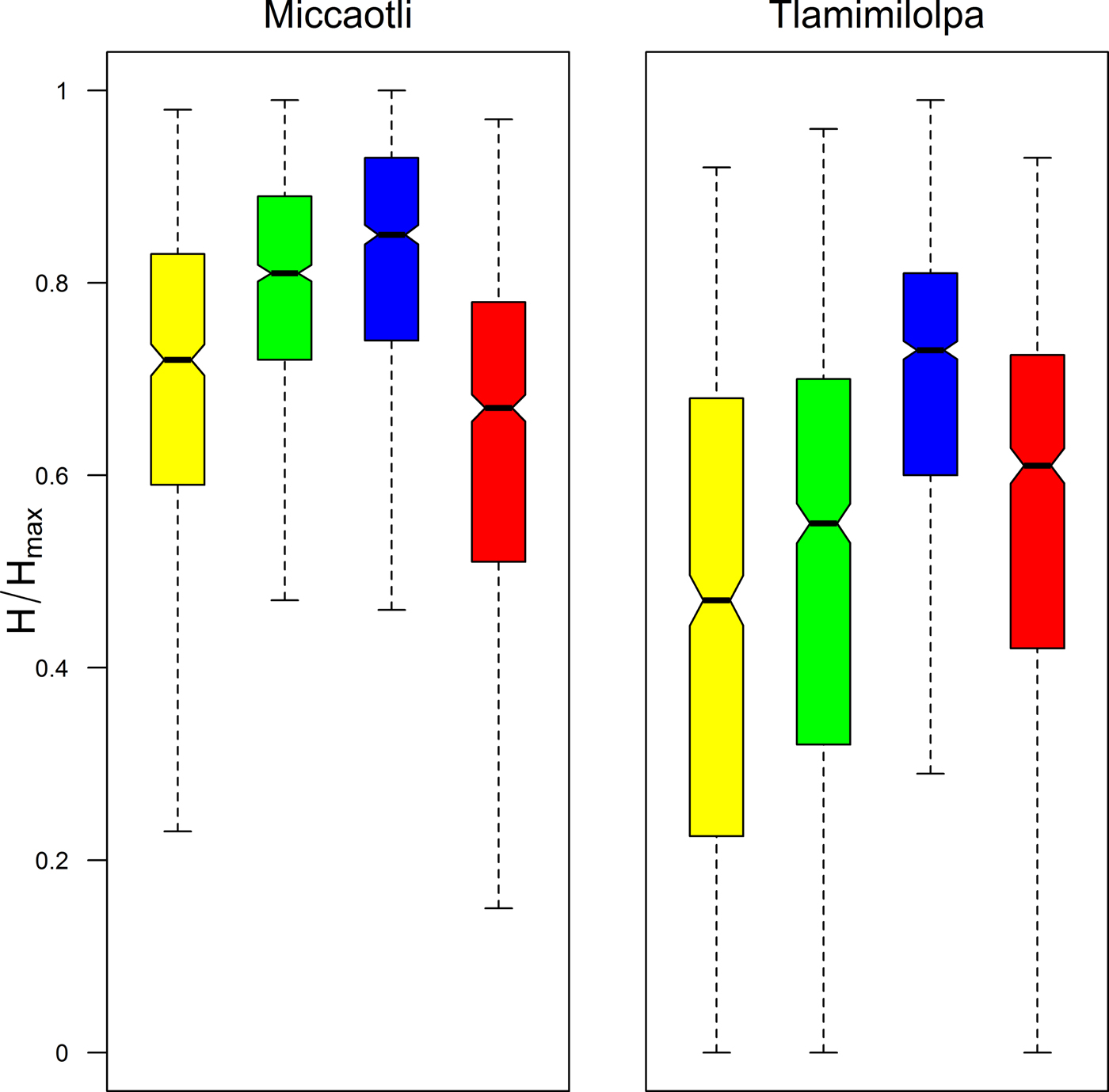
An important diachronic pattern revealed by this part of the study is a clear reduction in neighborhood diversity over time. Figure 8 illustrates the distribution of a quantitative measure of diversity, based on the evenness of the representation of the four wealth/status classes within each of the analytical neighborhoods used in the second stage of collection tract classification. Separate boxplots are provided for each of the two phases and the four neighborhood-level classes illustrated in Figures 6 and 7 (essentially, the social districts). The specific diversity measure shown is a standardized version of the Shannon index (J or H/Hmax; see Magurran Reference Magurran2004:108).

The boxplots show that Tlamimilolpa neighborhoods were, overall, more homogeneous than their Miccaotli counterparts, exhibiting greater domination by specific components of the wealth/status continuum, and hence, less even representation of the overall range of variation. This was particularly the case in the civic ceremonial zone, which, by the Tlamimilolpa phase, was overwhelmingly dominated by ceramic assemblages associated with households of high wealth/status levels. Less drastic changes in internal social diversity were exhibited by neighborhoods dominated by intermediate-status households. Peripheral parts of the city showed the least change; neighborhoods occupied largely by low-status households, mostly near the edge of the city, were only slightly less diverse in the Tlamimilolpa than in the Miccaotli phase.
The investigation I have been discussing aimed at elucidating aspects of Teotihuacan's socio-spatial structure by characterizing patterned variation in wealth and status at the level of individual structures, encompassing neighborhoods, and, as these latter contributed to higher-level spatial boundaries, still larger social districts. While the results have important implications for the social history of Teotihuacan, these can only be addressed here in the form of a brief summary. In short, although the diachronic changes revealed by comparing social diversity in Miccaotli- and Tlamimilolpa-phase neighborhoods reflect and relate to various factors, one of the most crucial was a shift in the relative importance of lineage, historical origins, and traditional leadership roles vs. status and wealth in determining social obligations and relationships of all kinds, but especially those facilitated by the residential proximity. I have argued further that physical reconfiguration of Teotihuacan's neighborhoods was likely facilitated by a crucial and even dramatic historical process: the widespread replacement during the Tlamimilolpa phase of existing residential structures with apartment compounds—with all the disruption and potential for socio-spatial manipulation that such a massive, large-scale project of urban renewal (Millon Reference Millon and Sabloff1981:209) must have entailed. Increasing wealth/status homogeneity in Teotihuacan's neighborhoods and social districts—and in particular the growth of a well-demarcated, elite-dominated zone around the ceremonial core—presumably reflects increasing social tensions that may have worked against long-term integration of the city. There is other evidence for social tensions growing over time (Sempowski Reference Sempowski and Berlo1992) and shifts in the socio-spatial landscape of this sort need to be considered as possible factors in the eventual collapse of Teotihuacan. Detailed interpretive discussions of these and other related issues can be found in Robertson (Reference Robertson2001, Reference Robertson, Gallut and Peralta2011b).
FINAL CONSIDERATIONS AND DISCUSSION
In spite of the theoretical importance of hinterland areas to the study of urban systems (Blanton Reference Blanton1976), I have been almost entirely concerned in this paper with information coming directly from Teotihuacan itself, and more specifically from the surface of the city as it was recorded by the Teotihuacan Mapping Project in the 1960s. The examples I used to illustrate ways in which these data have been employed over the years were selected to demonstrate the substantive and positive role that I feel they have already played and have the potential to play in future investigations of Teotihuacan.
As I noted at the beginning of this paper, however, not everyone regards surface collections as offering much potential for archaeological interpretation. The Real Mesoamerican Archaeologist was candidly negative: surface materials are simply “the junk you find on the surface—and nothing more. And I say, screw them” (Flannery Reference Flannery and Flannery1976:51). This assessment comes from an allegorical character, but similarly skeptical if less strident sentiments have been expressed about the value of surface data from Teotihuacan (for example, Gómez Chávez Reference Gómez Chávez1996:33; see also Hendon [Reference Hendon1992], Johnson [Reference Johnson2014], and Santley and Kneebone [Reference Santley, Kneebone, Santley and Hirth1993] for cautionary discussions about surface data based on work at other sites in Mesoamerica).
I do not have the space to take up the matter in any detail here. Cowgill (Reference Cowgill and Hammond1974:366–370, Reference Cowgill2015b) has carefully and objectively considered issues bearing on the suitability of TMP surface data for quantitative and other kinds of inferential reasoning in various places. He comes away cautiously optimistic overall, drawing attention, among other things, to the relatively shallow depth of cultural deposits over much of Teotihuacan and the often strong representation of early sherds even in areas where later occupations happen to have been very dense. Cowgill cites various examples of later subsurface investigations confirming both general and sometimes quite specific inferences made earlier on the basis of TMP surface data. My own views are similar and also summarized in substantial detail elsewhere (Robertson Reference Robertson2001:65–68). I confine myself below to some relatively simple observations that are to a large extent implicit in the preceding discussion and that have more to do with the nature of social patterning in cities than site-formation issues.
In short, many of the investigative themes that loom large in comparative studies of urbanism hinge on patterns that are most meaningfully expressed and understood at relatively large spatial scales, and that, simultaneously, are less likely to be recognized at small spatial scales or through spatially small windows of examination.
Most questions bearing on the internal organization of cities fall into this category, and a case in point is the multivariate investigation (into wealth/status variation, neighborhoods, and social districts at Teotihuacan) that I summarized at the end of the last section. In my view, the nested levels of spatial patterning that emerged from this work constitute important and fundamental elements in the internal organization of this preindustrial city and provide valuable points of comparison with other settlements (Smith Reference Smith2010). The crucial point here, however, is simply methodological: because of the scale of the phenomena in question it is difficult to imagine how similar insights could have been derived from anything but data from a carefully orchestrated (but also time-consuming and expensive) surface survey.
To be sure, some of the basic elements from which the broader socio-spatial pattern emerges are perfectly amenable to examination using subsurface data. The idea that wealthy and relatively poor households in Teotihuacan sometimes lived in close proximity, for example, was demonstrated in the 1990s by unusually extensive excavations in the La Ventilla district (Figure 1). There, two adjacent apartment compounds were documented, one only partially excavated, but apparently housing comparatively wealthy elites. The other compound was almost entirely exposed and generated rich information about the domestic living arrangements of the commoner artisans who lived within it (Cabrera Castro and Gómez Chávez Reference Cabrera Castro, Chávez, Mastache, Cobean, Cook and Hirth2008; Gómez Chávez Reference Gómez Chávez2000, Reference Gómez Chávez, Arnauld, Manzanilla and Smith2012). Critically, the narrow street that separated these compounds provided entry ways to both, but also had secondary modifications intended to control foot traffic through this common space. This suggests that some kind of special relationship, going beyond basic spatial proximity, existed between the two residential groups—most likely one specific manifestation of the general patron-client relationship I alluded to in my discussion (above) of the multivariate analysis of wealth/status variation.
Although the nature of any such relationship at La Ventilla remains unclear in many details, the excavations provide a level of resolution and interpretive detail that is entirely different from that generated by investigations based purely on surface data. Among other things, they serve as a form of ground truthing of a single, if fundamental element in a much broader and probably quite variable pattern. The fact that we can describe the latter as a “pattern,” however, is due entirely to analytical evidence based on spatially extensive surface data, as are insights into how it varied over time.
At this point in the discussion, I am probably belaboring a point that is straightforward and already obvious. In sum, in investigating Teotihuacan (or any other large, complex settlement), we need to make as much use as possible of at least two different kinds of information: relatively low-resolution but spatially extensive data recovered from the surface, and high-resolution but more focused information generated by subsurface excavation. These are complementary data that respectively provide context and detail, and much deeper insights when combined. Uneven consideration of the broader spatial context mars otherwise useful discussions of organizational phenomena (principally neighborhoods and districts) at Teotihuacan (Gómez Chávez Reference Gómez Chávez, Arnauld, Manzanilla and Smith2012; Manzanilla Reference Manzanilla, Arnauld, Manzanilla and Smith2012; Widmer and Storey Reference Widmer, Storey, Arnauld, Manzanilla and Smith2012).
The Future
A good case can be made that the importance of the TMP surface collections and data will grow instead of diminish over time. The reason for this is the accelerating rate of destruction of ancient Teotihuacan outside of the relatively small portion that is most directly and effectively protected by the Instituto Nacional de Antropología e Historia (INAH) of the Mexican government—the “Zona Arqueológica” that surrounds the ceremonial core and that covers between about 12% and 15% of the ancient city, depending on how one defines the outermost limits of the latter. Unfortunately, the Zona Arqueológica is where much and even most excavation has been conducted in recent decades, directed at sites facing no threats of imminent destruction. (Welcome exceptions in recent years include excavation work by Verónica Ortega in the “Oaxaca Barrio” [Ortega and Archer Reference Ortega Cabrera and Velasco2014]; by David Carballo and colleagues in the Tlajinga District; and by Oralia Cabrera Cortés (Reference Cabrera Cortés2006, 2010) and myself (Robertson Reference Robertson2008, Reference Robertson2011a) in different parts of the urban periphery of Teotihuacan.)
It is unclear how much more we will learn about Teotihuacan from fieldwork in more outlying districts. Although areas outside of the Zona Arqueológica are also subject to certain (lower) levels of official protection, a lack of both funding and effective enforcement means that urban sprawl and increasingly destructive agricultural practices are obliterating large parts of Teotihuacan at an alarming rate. If current trends continue, the main record remaining for much of the city will eventually be the artifacts and observations collected by Millon and his colleagues and co-workers in the 1960s. In the meantime, there is a great deal more that can and should be done with the legacy surface data created by the TMP, both in terms of data generation and management, as well as in the realm of exploratory and problem-oriented analysis.
With respect to the latter, although the TMP surface data are most directly a record of life within the capital of the Teotihuacan state, they have spatially broader implications stemming from the city's large ecological and demographic footprint. Larry Gorenflo and I have initiated a collaborative project that aims to mesh information derived from TMP records with parallel data from various regional surveys in surrounding parts of the Basin of Mexico (Gorenflo Reference Gorenflo2015). We aim, among other things, to characterize diachronic patterns of regional demographic flow, based for the first time on the most current and relatively complete settlement data available for urban Teotihuacan and the surrounding lake basin.
Returning to Teotihuacan itself, one might argue that in the immediate future we would do well to put as much energy as possible into excavation, above all in parts of the city, outside of the Zona Arqueológica, that are exposed to forces of unbridled development. There is a great deal of merit to this idea, and Cowgill's (Reference Cowgill2015b) paper in this same Special Section issue provides useful and specific suggestions. I would only emphasize the enhanced value of excavation that is strategic and problem-oriented; past and future analyses of TMP data could be an important source of specific hypotheses for, and a means of structuring, subsurface testing. As just one example, the social districts discussed above would be natural units for a stratified sampling program aimed at refining knowledge of socio-spatial variation in Teotihuacan through excavation.
Finally, in considering priorities for future fieldwork at Teotihuacan, I draw attention to one significant portion of the ancient city that was never systematically surveyed or recorded by the TMP. I refer to a zone extending outside the northwest corner of the official TMP survey grid (Figure 1), an area that may constitute as much as 4 km2 of additional urban terrain. Preliminary reconnaissance work showed that occupation there was largely confined to the Patlachique and Tzacualli phases (150 b.c.–a.d. 150). Since that zone was essentially abandoned afterward (at least for dense urban settlement), it was excluded from the formal TMP survey in order to focus efforts on generating a record of the “Classic” period city (Millon Reference Millon1973:8, Figure 13a and 13b; see also Sanders et al. Reference Sanders, West, Fletcher and Marino1975:191–192). Given the fact that so much of the architectural evidence for Patlachique and Tzacualli occupation was elsewhere obliterated by later construction, this zone remains a strategic place for investigating settlement and lifeways in early Teotihuacan. Although suffering from relatively high levels of erosion in some areas, modern urban sprawl and development seem to have impacted this part of the city more lightly than many other areas. A systematic survey and test excavation program there would make a tremendous contribution to existing TMP records, to Teotihuacan studies, and most broadly to our future understanding of Mesoamerican urbanism.
RESUMEN
En los años sesentas René Millon dirigió un programa de investigación de varios años enfocado en el centro urbano precolombino de Teotihuacan, en el centro de México. Además de crear un detallado mapa de la ciudad, el Teotihuacan Mapping Project (TMP) llevó a cabo un registro sistemático de los restos arqueológicos en superficie de aproximadamente 5,000 unidades de procedencia y durante su proceso, recolectó un total de aproximadamente un millón de artefactos arqueológicos. En su conjunto, los datos tanto descriptivos, como de los materiales mismos, recolectados por el TMP constituyen uno de los registros arqueológicos más extensivos y detallados que hayan sido creados para una ciudad antigua.
Este artículo proporciona una revisión y actualización de las observaciones de superficie del TMP, particularmente las que existen en formato digital. La organización del trabajo de campo y análisis del TMP se resumen poniendo énfasis en los factores que afectaron la naturaleza de los datos espaciales y descriptivos y la recuperación y análisis de las colecciones de materiales. Varios estudios específicos ilustran como los datos del TMP pueden ser usados a través del tiempo, incluyendo enfoques tanto espaciales como no espaciales.
Entre las innovaciones más recientes está el uso de sofisticados procedimientos de mapeo estadístico para identificar y describir patrones interpretables en la distribución de tipos de artefactos principales. Como un ejemplo interesante, se presentan los mapas temáticos basados en medidas relacionadas con el concepto de autocorrelación espacial aplicados a dos de las formas cerámicas principales de la loza Anaranjando San Martín (SMO), los cráteres y las ánforas. Los mapas revelan diferencias marcadas entre las dos formas de vasijas; además, los patrones espaciales de las ánforas SMO involucran esta forma cerámica de manera convincente en actividades económicas centradas en la obtención de la savia del maguey (aguamiel y pulque), particularmente en las zonas periféricas del oeste de la ciudad.
El potencial para explotar los datos del TMP usando métodos estadísticos multivariantes para identificar barrios y otros tipos de entidades espaciales característicos de los asentamientos urbanos se reconoció hace décadas, y se han llevado a cabo varias investigaciones en este sentido. Un estudio examinado en este artículo adopta un enfoque de clasificación de dos etapas. La primera lleva a cabo una caracterización de los patrones de variación socio-espacial en los vecindarios Teotihuacanos, y la segunda usa la variación espacial en la composición de vecindarios para delimitar distritos sociales más grandes. Los resultados claramente muestran que antes de la adopción de los conjuntos departamentales, los vecindarios residenciales en Teotihuacan fueron relativamente heterogéneos en términos de composición de riqueza/estatus, creciendo posteriormente de manera mucho más homogénea. Al mismo tiempo, los distritos sociales se tornaron en entidades más coherentes y espacialmente mejor delimitadas, con zonas diferentes en la ciudad cada vez más dominadas numéricamente por gente de más o menos de la misma riqueza/estatus. Los resultados del análisis tienen implicaciones importantes para entender la estructura social urbana de Teotihuacan, la amplia adopción de los conjuntos departamentales, y la supervivencia a largo plazo de Teotihuacan como una ciudad integrada social y políticamente.
La conclusión más general de este artículo es que los datos espaciales extensivos generados por proyectos de prospección y recolección de materiales de superficie bien planeados y ejecutados, son cruciales para investigar elementos de la organización de los asentamientos urbanos, sobre todo las entidades espaciales tales como los vecindarios y los distritos sociales. Su valor es acrecentado considerablemente cuando se integra con problemas orientados a la investigación basada en excavaciones. En este caso específico, la importancia del legado de los datos del TMP para investigar Teotihuacan probablemente—y desafortunadamente—solo aumentará más con el tiempo, mientras que partes más y más grandes de la ciudad, que están fuera de la protección directa de la Zona Arqueológica, se pierdan permanente frente a las fuerzas aparentemente imparables de la urbanización moderna y los cambios del uso de suelo.
ACKNOWLEDGMENTS
I thank attendees at the Ometusco Seminar both for their energetic participation in that meeting and for feedback on the material that I presented there. The latter forms the basis for the current paper and I am grateful to Larry J. Gorenflo for his very helpful comments, advice, and encouragement on an early draft. I thank George L. Cowgill for comments on a later version, and Carrie Dennett, Nancy Gonlin, and two anonymous reviewers for thoughtful and detailed feedback during the review process. Oralia Cabrera kindly translated my Spanish abstract.