1. Introduction
The angular dynamics of small non-spherical particles advected in turbulence and other mixing flows is a subject of significant recent interest (Wilkinson, Bezuglyy & Mehlig Reference Wilkinson, Bezuglyy and Mehlig2009; Parsa et al. Reference Parsa, Calzavarini, Toschi and Voth2012; Chevillard & Meneveau Reference Chevillard and Meneveau2013; Gustavsson, Einarsson & Mehlig Reference Gustavsson, Einarsson and Mehlig2014; Ni, Ouelette & Voth Reference Ni, Ouelette and Voth2014; Byron et al. Reference Byron, Einarsson, Gustavsson, Voth, Mehlig and Variano2015; Zhao et al. Reference Zhao, Challabotla, Andersson and Variano2015; Einarsson et al. Reference Einarsson, Mihiretie, Laas, Ankardal, Angilella, Hanstorp and Mehlig2016; Hejazi, Mehlig & Voth Reference Hejazi, Mehlig and Voth2017; Voth & Soldati Reference Voth and Soldati2017; Zhao et al. Reference Zhao, Gustavsson, Ni, Kramel, Voth, Andersson and Mehlig2019). In these studies it is assumed that the particles are small enough so that inertial effects can be neglected (Subramanian & Koch Reference Subramanian and Koch2005; Einarsson, Angilella & Mehlig Reference Einarsson, Angilella and Mehlig2014; Einarsson et al. Reference Einarsson, Candelier, Lundell, Angilella and Mehlig2015; Rosén et al. Reference Rosén, Einarsson, Nordmark, Aidun, Lundell and Mehlig2015), but the particles are large enough to neglect rotational diffusion (Hinch & Leal Reference Hinch and Leal1972). In this creeping-flow limit, the equation of motion for the angular dynamics was derived by Jeffery (Reference Jeffery1922). Jeffery's theory describes the angular dynamics of spheroidal particles in terms of their shape and the local fluid-velocity gradients.
It is usually assumed that the particles are axisymmetric, which means that they have an axis of continuous rotational symmetry, and that they possess fore-and-aft symmetry. In this case the main interest lies in the dynamics of the director  $\boldsymbol {n}$ that points along the symmetry axis of the particle. The question is how it tumbles in response to the fluid-velocity gradients. How such particles spin around their symmetry axis
 $\boldsymbol {n}$ is usually not considered. One reason is that the spin is more difficult to measure in experiments, for axisymmetric particles.
The shape of an axisymmetric particle with fore-and-aft symmetry is parameterised by its aspect ratio  $\lambda =a/b$, defined here as the ratio of the symmetry-axis length
 $2 a$ to the diameter
 $2 b$ of the particle. Prolate particles have
 $\lambda >1$ while oblate particles have
 $\lambda < 1$. Jeffery considered spheroids (amongst other shapes), and showed that particle shape enters the angular dynamics in the creeping-flow limit only through the shape parameter (Jeffery Reference Jeffery1922; Bretherton Reference Bretherton1962)
 \begin{equation} \Lambda = \frac{\lambda^2-1}{\lambda^2+1}. \end{equation}
The shape parameters  $\Lambda =0, 1, -1$ correspond to spherical particles, infinitely slender rods and infinitely thin discs, respectively.
The studies of particles in turbulence mentioned above refer to homogeneous and isotropic turbulent flows, or to statistical models for such flows. Due to isotropy, such flows do not possess a preferred orientation in the laboratory frame. But it turns out that the particles align with local directions in the flow in intricate ways, not all of them fully understood. Pumir & Wilkinson (Reference Pumir and Wilkinson2011) used direct numerical simulation (DNS) of homogeneous, isotropic turbulence to show that infinitely slender particles tend to align with the fluid vorticity vector. The vorticity vector is defined as the curl of the fluid velocity. Many authors (Guala et al. Reference Guala, Lüthi, Liberzon, Tsinober and Kinzelbach2005; Pumir & Wilkinson Reference Pumir and Wilkinson2011; Parsa et al. Reference Parsa, Calzavarini, Toschi and Voth2012; Chevillard & Meneveau Reference Chevillard and Meneveau2013; Gustavsson et al. Reference Gustavsson, Einarsson and Mehlig2014; Ni et al. Reference Ni, Ouelette and Voth2014) have analysed how vorticity and slender particles align with the orthogonal system of eigenvectors of the local fluid strain-rate matrix. These studies show that both slender particles, and vorticity, align weakly with this frame. Of the three eigenvectors, a slender rod aligns best with the intermediate eigenvector, to a lesser extent with the maximal eigenvector, and almost orthogonal to the minimal eigenvector. This result is surprising because it is natural to expect a slender particle to align best with the maximal eigendirection. This puzzle was resolved by Xu, Pumir & Bodenschatz (Reference Xu, Pumir and Bodenschatz2011) who explained that the orientation of an infinitely slender particle tends to follow the maximal eigendirection of the strain-rate matrix, but that the eigensystem of the strain-rate matrix rotates away as the slender particle turns. In other words, non-intuitive alignment with respect to the eigensystem of the strain-rate matrix is a consequence of the fact that the time scales of the turbulent dynamics and that of the orientation of infinitely slender rods are similar.
A third local reference frame is formed by the principal axes of deformation of a fluid element. An infinitesimal, spherical volume of fluid deforms with time into an ellipsoid. The principal axes of this ellipsoid form an orthogonal coordinate system. The principal axis corresponding to the direction of largest stretching defines the Lagrangian stretching direction. The alignment of the Lagrangian stretching direction has been investigated in the frame of the eigenvectors of the fluid strain-rate matrix. Girimaji & Pope (Reference Girimaji and Pope1990) found imperfect alignment of the Lagrangian stretching direction with the maximal eigenvector of the fluid strain-rate matrix. This was because the eigenvectors of the strain-rate themselves rotated with time (Drummond & Münch Reference Drummond and Münch1990; Girimaji & Pope Reference Girimaji and Pope1990; She et al. Reference She, Jackson, Orszag, Hunt, Phillips and Williams1991). The DNS results of Johnson et al. (Reference Johnson, Hamilton, Burns and Meneveau2017) showed that near the centre of a turbulent channel flow, similar to homogeneous, isotropic turbulence, the Lagrangian stretching direction aligns best with the intermediate eigenvector of the strain-rate matrix. Near the channel wall, however, the alignment is strongest with the maximal eigenvector.
Compared to vorticity and the eigensystem of the strain-rate matrix, a simpler picture emerges if one describes local alignment of the rod direction with the eigensystem of the left Cauchy–Green tensor (Wilkinson et al. Reference Wilkinson, Bezuglyy and Mehlig2009; Bezuglyy, Mehlig & Wilkinson Reference Bezuglyy, Mehlig and Wilkinson2010; Wilkinson, Bezuglyy & Mehlig Reference Wilkinson, Bezuglyy and Mehlig2011; Ni et al. Reference Ni, Ouelette and Voth2014; Hejazi et al. Reference Hejazi, Mehlig and Voth2017). There are two reasons for this simplicity. First, the direction of infinitely slender rods must converge to the leading eigenvector of the left Cauchy–Green tensor, and second, even though the eigenvalues of this tensor are not statistically stationary, the eigenvectors become independent of the initial conditions after an initial transient (Batchelor Reference Batchelor1952; Balkovsky & Fouxon Reference Balkovsky and Fouxon1999).
One recurring observation is that the alignment of axisymmetric particles in homogeneous and isotropic turbulent flows is quite insensitive to particle shape for values of  $|\Lambda |$ close to unity. Parsa et al. (Reference Parsa, Calzavarini, Toschi and Voth2012), for instance, showed (see figure 3c in that paper) that the root mean square tumbling rate
 $\langle | \dot {\boldsymbol {n}}|^2\rangle$ in turbulence becomes roughly independent of shape for
 $|\Lambda |> 0.8$. Ni et al. (Reference Ni, Ouelette and Voth2014) showed that slender rods with aspect ratio
 $\lambda =20$ (
 $\Lambda = 0.995$) follow the Lagrangian stretching direction of the turbulent flow quite closely, see figure 1(a) in that paper. Parsa et al. (Reference Parsa, Guasto, Kishore, Ouellette, Gollub and Voth2011) concluded that in two-dimensional chaotic flows, rods preferentially align with the Lagrangian stretching direction, and that the alignment is nearly independent of the length of the rods. Related conclusions have been drawn for active particles. Dehkharghani et al. (Reference Dehkharghani, Waisbord, Dunkel and Guasto2019) considered motile bacteria with effective aspect ratio
 $\lambda =10$ in an inhomogeneous flow, with discrete translational symmetry, and used the Lagrangian stretching direction as a proxy for orientational alignment of the slender bacteria. Borgnino et al. (Reference Borgnino, Gustavsson, De Lillo, Boffetta, Cencini and Mehlig2019) found that active particles such as motile bacteria tend to align with the instantaneous fluid velocity. The conclusion is, in other words, that slender rods align well with the Lagrangian stretching direction, and that the alignment is not very sensitive to their aspect ratio in homogeneous isotropic turbulence. However, the precise dependence of this alignment on the shape parameter of the particle is not understood.
The presence of bounding walls for turbulent flows, however, breaks homogeneity and isotropy. A natural question to ask is how the presence of walls affects the alignment behaviour of slender rods? Zhao & Andersson (Reference Zhao and Andersson2016) found that elongated rods in a turbulent channel flow align preferentially with the Lagrangian stretching direction, but that the orientation and rotation behaviours appear to depend quite sensitively upon the aspect ratio near the wall (Challabotla, Zhao & Andersson Reference Challabotla, Zhao and Andersson2015; Zhao et al. Reference Zhao, Challabotla, Andersson and Variano2015). Several authors have analysed how the orientation of slender rods aligns with the laboratory-fixed basis of a turbulent channel flow. The results were summarised by Voth & Soldati (Reference Voth and Soldati2017). Briefly, in the near-wall turbulence the slender rods were found to preferentially align in the streamwise direction (Mortensen et al. Reference Mortensen, Andersson, Gillissen and Boersma2008; Marchioli, Fantoni & Soldati Reference Marchioli, Fantoni and Soldati2010) but thin disks tend to align in the wall-normal direction (Zhao & Andersson Reference Zhao and Andersson2016). But near the channel wall vorticity aligns preferentially with the spanwise direction due to the presence of mean shear (Zhao & Andersson Reference Zhao and Andersson2016) and thus does not describe alignment of slender rods. In the case of turbulent channel flows, precisely which mechanisms lead to alignment between slender rods and the Lagrangian stretching direction is not understood. Similar to the case of homogeneous, isotropic turbulence, another open question is how the alignment depends on the shape parameter of the particle.
One motivation for studying particles in a turbulent channel flow is that this problem is relevant for industrial applications. An example is the flow of fibre suspensions in papermaking (Lundell, Söderberg & Alfredsson Reference Lundell, Söderberg and Alfredsson2011). Such fibres are typically very slender. The fibres in the experimental study of Carlsson, Söderberg & Lundell (Reference Carlsson, Söderberg and Lundell2010) are  $0.7$ mm long on average, with average diameter
 $18\ \mathrm {\mu }$m. This corresponds to
 $\Lambda = 0.999$, very close to unity. Further, industrial flows are usually inhomogeneous and lack isotropy, certainly near the walls that contain them. In a turbulent channel flow near the channel centre the turbulent velocity-gradient fluctuations are approximately homogeneous and isotropic, but near the wall the fluid velocity-gradient fluctuations are anisotropic in addition to having a large mean shear component.
We therefore investigate the alignment statistics of relative angles between a small slender rod and the Lagrangian stretching direction in a turbulent channel flow. We study how the distribution of relative angles depends on the particle aspect ratio and on the distance of the particle from the channel wall. Our numerical studies employ DNS of a turbulent channel flow with a friction Reynolds number  $Re_\tau =180$ (Challabotla et al. Reference Challabotla, Zhao and Andersson2015).
Overall we find that the distribution of relative angles between the orientation of a slender rod and the Lagrangian stretching direction has a power-law tail for large angles, cut off by a plateau of width  $\delta \Lambda = 1-\Lambda$ at small angles. Since we consider directors symmetric under reflection, the relative angle is bounded between
 $-{\rm \pi} /2$ and
 $+{\rm \pi} /2$. This means that a clear power-law tail is observed only when
 $\delta \Lambda \ll {\rm \pi}/2$. In fact, for the largest value
 $\delta \Lambda = 0.1$ which we have considered, the power-law tails are not so clear. When the relative angular separation between a thin rod and the Lagrangian stretching direction is small, the orientations of the two are essentially uncorrelated. However, in rare cases, the relative angle can show excursions to large angles followed by relaxation back to small angles. These large excursions give rise to power-law tails in the distribution of the angle between the rod orientation and the Lagrangian stretching direction. The width of the plateau describes the variance of the relative angles and depends on the shape parameter,
 $\Lambda$, of the rod as well as the distance of the particle from the channel wall. For the same shape parameter
 $\Lambda$, we find that the plateau is broader near the channel wall than near the channel centre, indicating that a slender rod exhibits stronger alignment with the Lagrangian stretching direction near the channel centre than near the channel wall.
We explain the observations using idealised statistical models for relative angles based on Jeffery's equation. The models assume that the fluid-velocity gradients experienced by the tracer rod fluctuate rapidly (Gustavsson et al. Reference Gustavsson, Berglund, Jonsson and Mehlig2016). This white-noise limit has also proved useful in understanding the dynamics of relative separations of spherical particles in turbulence (see Gustavsson et al. (Reference Gustavsson, Berglund, Jonsson and Mehlig2016) for a review) and has been used to study relative angles between nearby rods in turbulence (Zhao et al. Reference Zhao, Gustavsson, Ni, Kramel, Voth, Andersson and Mehlig2019). In turbulence, near the channel centre, the fluid-velocity gradients fluctuate on the same time scale as the angular dynamics of slender rods. Yet, our approximation preserves the qualitative behaviour of relative angle dynamics because the time scale of particle angular dynamics and the Lagrangian stretching direction are independent of the time scale of velocity-gradient fluctuations. However, our model for the channel centre is two-dimensional, and so it is merely a caricature of the complete three-dimensional problem. By contrast, near the channel wall, the white-noise limit turns out to be a good approximation due to the slow angular dynamics of slender rods in strong mean shear. This allows us to obtain quantitatively accurate results. Our models are obtained by linearising the equations of motion in the relative angle, and thus are subject to the regime of validity of this assumption. Near the channel centre we find the model works well up to  $\delta \Lambda \sim O(10^{-1})$. Near the channel wall, the regime of validity is described by the ratio of the strength of velocity-gradient fluctuations to the mean shear-rate.
The equation of motion that we obtain for the relative angle is analogous to a stochastic differential equation with additive and multiplicative noises. Mathematically, the observed plateau and power-law tails are a consequence of the additive and multiplicative terms, respectively (Kesten Reference Kesten1973; Deutsch Reference Deutsch1994; Gustavsson, Mehlig & Wilkinson Reference Gustavsson, Mehlig and Wilkinson2015). However, the physical mechanism leading to large excursions near the channel centre is completely different from the mechanism near the channel wall. Near the channel centre the relative angular dynamics are purely diffusive. The corresponding diffusion coefficient increases with the angular separation. Near the channel wall, on the other hand, the dynamics are a result of the weak velocity-gradient fluctuations and the strong mean shear. The weak velocity-gradient fluctuations modify both the width of the plateau and the power-law exponent in the steady-state distribution of relative angles compared with the case of shear without fluctuations.
The remainder of this paper is organised as follows. In § 2 we briefly describe the background, explaining what is known about the alignment of rods in turbulent flows, introducing our notation and describing the numerical method for DNS of channel flow. Section 3 summarises the results of our DNS studies, characterising the alignment of the particle-orientation vector  $\boldsymbol {n}$ with the Lagrangian stretching direction near the channel centre and near the wall. In § 4 we explain the observations near the channel centre qualitatively, and near the channel wall quantitatively by using simple models based on Jeffery's equation. In § 5 we discuss the consequences of our findings for the problem of angular structure functions. Section 6, finally, contains our conclusions.
2. Background
2.1. Angular dynamics of axisymmetric particles in turbulence
The centre of mass of small inertialess particles simply follows the flow
 \begin{equation} \dot{\boldsymbol{x}} = \boldsymbol{u}(\boldsymbol{x}(t),t), \end{equation}
assuming that spatial diffusion is negligible. Here  $\boldsymbol {x}(t)$ is the centre of mass position of the particle at time
 $t$, and
 $\boldsymbol {u}(\boldsymbol {x}(t),t)$ is the fluid velocity at the particle position at time
 $t$. The orientation
 $\boldsymbol {n}$ of an axisymmetric, rigid particle with shape parameter
 $\Lambda$ follows Jeffery's equation (Jeffery Reference Jeffery1922)
 \begin{equation} \dot{\boldsymbol{n}} = {\boldsymbol{B}}(\boldsymbol{x}(t),t) \boldsymbol{n} - [\boldsymbol{n} \boldsymbol{\cdot}{\boldsymbol{B}}(\boldsymbol{x}(t),t)\boldsymbol{n}]\boldsymbol{n}, \end{equation}
with  ${\boldsymbol{B}} = {\boldsymbol{O}} +\Lambda {\boldsymbol{S}}$, where
 ${\boldsymbol{O}}$ and
 ${\boldsymbol{S}}$ are the antisymmetric and symmetric parts of the fluid-gradient matrix
 ${\boldsymbol{A}}$.
As mentioned in the introduction, effects of rotational diffusion and rotational inertia are neglected in Jeffery's theory. We note that (2.2) holds not only for particles with continuous rotational symmetry, but also for crystals with discrete point-group symmetries (Fries, Einarsson & Mehlig Reference Fries, Einarsson and Mehlig2017; Fries et al. Reference Fries, Kumar, Mihiretie, Hanstorp and Mehlig2018), although there is no general formula for the parameter  $\Lambda$ in terms of particle dimensions and shape.
In order to obtain the Lagrangian stretching direction, first one defines the deformation tensor  ${\boldsymbol{D}}$ as the solution of the differential equation
 \begin{equation} \frac{\textrm{d}}{\textrm{d}t} {\boldsymbol{D}}(t)= {\boldsymbol{A}}(t) {\boldsymbol{D}}(t), \quad\mbox{with initial condition } {\boldsymbol{D}}(0) = \mathbb{1}. \end{equation}
The left Cauchy–Green tensor  ${\boldsymbol{M}}(t)$ is then formed as
 ${\boldsymbol{M}} = {\boldsymbol{D}} {\boldsymbol{D}}^{\textsf T}$. The tensor
 ${\boldsymbol{M}}(t)$ is symmetric with eigenvalues
 $\sigma _1(t) > \sigma _2(t)> \sigma _3(t)> 0$, and eigenvectors
 $\hat {\boldsymbol {e}}_{{L}1}(t), \hat {\boldsymbol {e}}_{{L}2}(t), \hat {\boldsymbol {e}}_{{L}3}(t)$. The leading eigenvector
 $\hat {\boldsymbol {e}}_{{L}1}(t)$ corresponding to the largest eigenvalue
 $\sigma _1$ is called Lagrangian stretching direction, while the eigenvector
 $\hat {\boldsymbol {e}}_{{L}3}$ corresponding to the smallest eigenvalue
 $\sigma _3$ is the compressing direction. The middle eigenvector,
 $\hat {\boldsymbol {e}}_{{L}2}$, forms an orthonormal coordinate system with the other two. In the case of an incompressible flow,
 ${Tr} {\boldsymbol{A}} =0$ so that the eigenvalues of the left Cauchy–Green tensor satisfy
 $\sigma _1\sigma _2\sigma _3=1$. In the long-time limit, the equation of motion of the Lagrangian stretching direction
 $\hat {\boldsymbol {e}}_{{L}1}(t)$ (Balkovsky & Fouxon Reference Balkovsky and Fouxon1999) reduces to the equation for
 $\boldsymbol {n}(t)$ given by (2.2) for an infinitely slender rod,
 $\Lambda =1$. Further, in the long-time limit, an infinitely slender rod aligns perfectly with the Lagrangian stretching direction.
But how well do rods with finite aspect ratios follow the Lagrangian stretching direction? In other words, how sensitive is the angular dynamics to small deviations  $\delta \Lambda$ from
 $\Lambda =1$? To quantify this we compute the steady-state distribution of the Euler angles
 $\alpha$ and
 $\beta$ that quantify the angular separations between the orientation vector
 $\boldsymbol {n}$ and
 $\hat {\boldsymbol {e}}_{{L}1}$ in the
 $\hat {\boldsymbol {e}}_{{L}1}\text {--}\hat {\boldsymbol {e}}_{{L}3}$ plane (yaw) and out of the
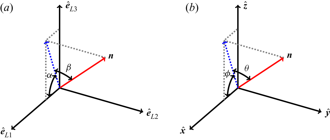
 $\hat {\boldsymbol {e}}_{{L}1}\text {--}\hat {\boldsymbol {e}}_{{L}3}$ plane (pitch), respectively, as shown in figure 1(a). The surface element for the angles
 $\alpha , \beta$ on the unit sphere is
 $\cos \beta \, \textrm {d} \alpha \, \textrm {d} \beta$. Thus, a uniform distribution of orientations on the unit sphere corresponds to
 $P(\alpha ,\beta ) \propto \cos \beta$. Consequently, the uniform marginal distributions corresponding to angles
 $\alpha$ and
 $\beta$ are
 $P(\alpha ) = \text {const.}$ and
 $P(\beta ) \propto \cos \beta$, respectively. Note that for
 $\beta \ll 1, \cos \beta \approx 1$ and thus for angles smaller than order unity, one may safely approximate
 $P(\beta ) \sim \text {const.}$ as the reference uniform distribution of the angle
 $\beta$.
Euler angles used in analysing the alignment of the particle-symmetry vector  $\boldsymbol {n}$. (a) Coordinate system defined by the eigenvectors
 $\hat {\boldsymbol {e}}_{{L}1}(t),\, \hat {\boldsymbol {e}}_{{L}2}(t)\ {\rm and}\ \hat {\boldsymbol {e}}_{{L}3}(t)$ of the left Cauchy–Green tensor
 ${\boldsymbol {M}}(t)$. Here
 $\hat {\boldsymbol {e}}_{{L}1}$ and
 $\hat {\boldsymbol {e}}_{{L}3}$ are the expanding and contracting directions, while
 $\hat {\boldsymbol {e}}_{{L}2}$ is chosen to keep the coordinate system right-handed, and
 $\alpha$,
 $\beta$ are Euler angles in this reference frame. (b) Fixed Cartesian channel-coordinate system with basis vectors
 $\hat {\boldsymbol {x}}, \hat {\boldsymbol {y}}$ and
 $\hat {\boldsymbol {z}}$. Here
 $\hat {\boldsymbol {x}}$ is the streamwise direction,
 $\hat {\boldsymbol {y}}$ the spanwise, and
 $\hat {\boldsymbol {z}}$ the wall-normal direction of the channel flow. The Euler angles are
 $\phi$ and
 $\theta$.

In the laboratory frame of the turbulent channel flow, we define  $\hat {\boldsymbol {x}}$ to be the flow direction,
 $\hat {\boldsymbol {y}}$ to be the spanwise direction and
 $\hat {\boldsymbol {z}}$ to be the wall-normal direction. Euler angles
 $\theta$ and
 $\phi$ are defined, respectively, as the angle between the orientation vector
 $\boldsymbol {n}$ and the
 $\hat {\boldsymbol {x}}\text {--}\hat {\boldsymbol {z}}$ plane, and the angle between the projection of
 $\boldsymbol {n}$ in the
 $\hat {\boldsymbol {x}}\text {--}\hat {\boldsymbol {z}}$ plane and
 $\hat {\boldsymbol {x}}$, see figure 1(b).
We define two different coordinate systems because even though the goal is to understand angular dynamics in the frame defined by the eigenvectors of the left Cauchy–Green tensor, statistical model calculations are more tractable in the laboratory frame. All DNS results compute the distributions of angles  $\alpha , \beta$ directly. In § 4, we use statistical models to analytically understand the distributions of relative angles. Near the channel centre we use a two-dimensional toy model to analytically calculate the distribution of the angle
 $\alpha$. Near the channel wall we compute the joint distribution of
 $\phi , \delta \phi$ for a simple statistical model.
2.2. DNS of channel flow
We perform DNS of a turbulent channel flow at  $Re_\tau = 180$. The friction Reynolds number is defined as
 $Re_\tau = h u_\tau / \nu$, where
 $h$ is the channel half-height,
 $u_\tau$ is the wall friction velocity and
 $\nu$ is the kinematic viscosity of the fluid. We choose a domain of size
 $12h\times 6h\times 2h$ with 192 grid points in the streamwise (
 $\hat {\boldsymbol {x}}$), spanwise (
 $\hat {\boldsymbol {y}}$) and wall-normal (
 $\hat {\boldsymbol {z}}$) directions, respectively. Periodic boundary conditions are imposed in the homogeneous
 $\hat {\boldsymbol {x}}$ and
 $\hat {\boldsymbol {y}}$ directions and the no-slip and impermeability conditions are imposed at the walls. In the following, the subscript
 $+$ denotes normalisation by the viscous scales, i.e. the viscous length scale
 $\nu /u_\tau$ and viscous time scale
 $\nu /u_\tau ^2$. The corresponding grid resolution is uniform in the streamwise and spanwise directions, with grid spacings
 ${\rm \Delta} x^+ = 11.3$ and
 ${\rm \Delta} y^+ = 5.6$. The grid in the wall-normal direction is refined near the wall, and the spacing
 ${\rm \Delta} z^+$ is 0.9 at the channel walls, but increases to 2.86 at channel centre. A pseudo-spectral method is applied along the homogeneous directions and a second-order finite-difference discretisation is used in the wall-normal direction. Time integration is performed using a second-order explicit Adams–Bashforth scheme with time step
 ${\rm \Delta} t^+= 0.036$ (Zhao & Andersson Reference Zhao and Andersson2016).
Our simulations show nearly homogeneous and isotropic turbulence near the channel centre (Andersson, Zhao & Variano Reference Andersson, Zhao and Variano2015). Near the channel wall, however, the flow is anisotropic (Mansour, Kim & Moin Reference Mansour, Kim and Moin1988; Pumir Reference Pumir2017). In particular, the no-slip boundary conditions induce a large mean shear near the wall and low/high speed streaks are formed in the near-wall region and have been observed in both experiment and numerical simulations (Kim, Moin & Moser Reference Kim, Moin and Moser1987). The near-wall turbulence structures and the presence of shear play important roles for inertial particle accumulation (Marchioli & Soldati Reference Marchioli and Soldati2002) and particle rotation (Zhao et al. Reference Zhao, Challabotla, Andersson and Variano2015).
3. DNS results
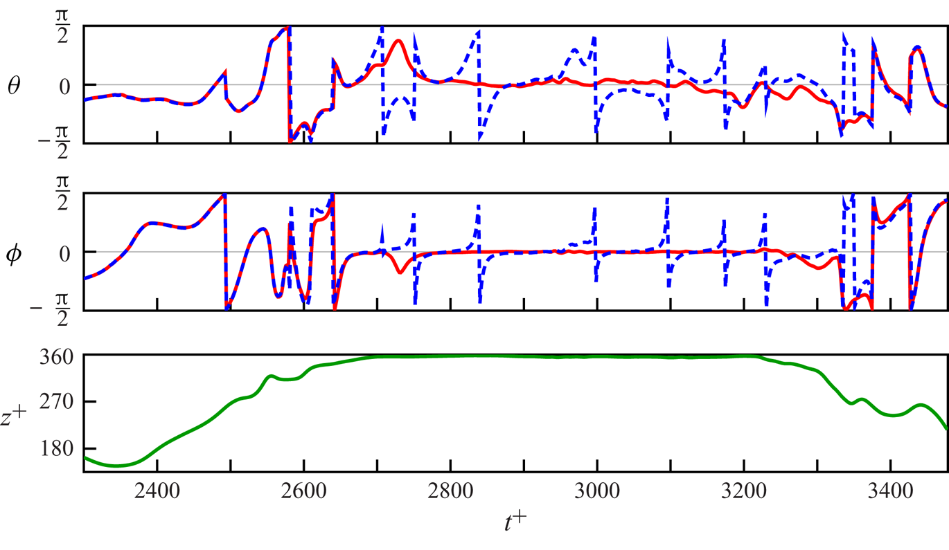
Figure 2 shows DNS results for the angular dynamics of the orientation  $\boldsymbol {n}(t)$ of a slender rod (
 $\Lambda = 0.9963$) in the channel flow, compared with the angular dynamics of the Lagrangian stretching direction
 $\hat {\boldsymbol {e}}_{{L}1}(t)$. Figure 2 demonstrates that
 $\boldsymbol {n}(t)$ aligns quite well with the Lagrangian stretching direction when the particle is near the centre of the channel. This observation is consistent with findings in a two-dimensional chaotic flow (Parsa et al. Reference Parsa, Guasto, Kishore, Ouellette, Gollub and Voth2011) and in homogeneous isotropic turbulence (Ni et al. Reference Ni, Ouelette and Voth2014). But when the particle is near the wall, the angular dynamics of
 $\boldsymbol {n}(t)$ and
 $\hat {\boldsymbol {e}}_{{L}1}(t)$ seem to be different: while
 $\boldsymbol {n}(t)$ tumbles in the near-wall shear flow, the Lagrangian stretching direction aligns with the streamwise direction,
 $\hat {\boldsymbol {x}}$. Small deviations are due to fluid-velocity gradient fluctuations, but they do not seem to cause
 $\hat {\boldsymbol {e}}_{{L}1}(t)$ to tumble. The alignment behaviour with respect to the channel coordinate frame exhibited by the slender rod (
 $\Lambda = 0.9963$) in figure 2 is consistent with the streamwise and spanwise alignment of slender rods reported by Challabotla et al. (Reference Challabotla, Zhao and Andersson2015), see figure 2 in that paper.
Angular dynamics of a slender rod in the turbulent channel flow. The top two panels show the Euler angles  $\theta$ and
 $\phi$, see figure 1(b), of the Lagrangian stretching direction
 $\hat {\boldsymbol {e}}_{{L}1}(t)$ (solid red line) and of the orientation vector
 $\boldsymbol {n}(t)$ of a particle with
 $\Lambda = 0.9963$ (blue dashed line). The bottom panel shows the
 $z$-coordinate of the centre of mass position of the particle in the channel. The bottom boundary of channel is located at
 $z^+ = 0$, the centreline at
 $z^+=180$ and the top boundary at
 $z^+=360$. During the time interval
 $2700 < t^+ < 3200$ the particle travels in the viscous boundary layer,
 $z^+>355$, near the top boundary.

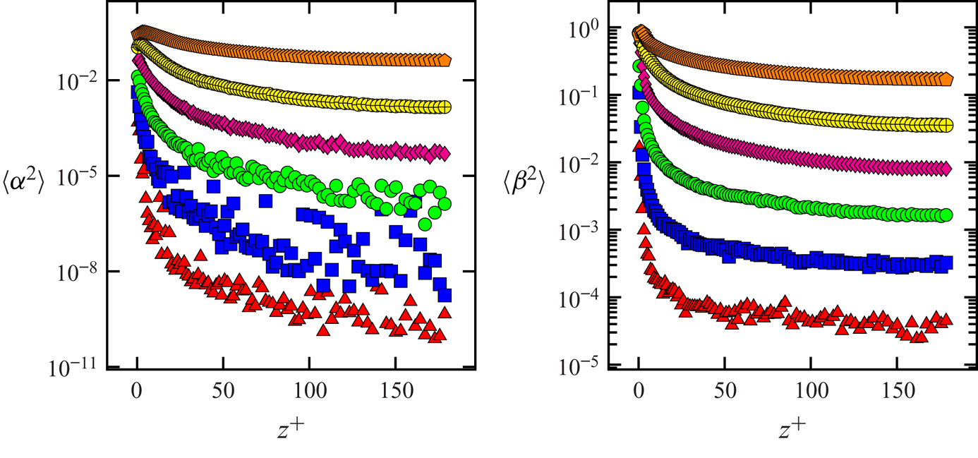
In order to investigate and quantify this difference, we compute the probability distributions of the angles  $\alpha$ and
 $\beta$ near the centre (see figure 3) and near the wall (see figure 4). The angles
 $\alpha$ and
 $\beta$ characterise the difference between the particle orientation vector
 $\boldsymbol {n}(t)$ and the Lagrangian stretching direction
 $\hat {\boldsymbol {e}}_{{L}1}(t)$. We expect
 $\beta$ to show larger fluctuations than
 $\alpha$. This is because
 $\alpha$ measures the relative angle in the plane of the Lagrangian stretching direction and the maximal contracting direction (
 $\hat {\boldsymbol {e}}_{{L}3}$), and so is controlled by the corresponding eigenvalues
 $\sigma _1$ and
 $\sigma _3$. By contrast,
 $\beta$ measures the relative angle out of the
 $\hat {\boldsymbol {e}}_{{L}1}\text {--}\hat {\boldsymbol {e}}_{{L}3}$ plane and thus
 $\beta$ is influenced by the intermediate eigenvalue,
 $\sigma _2$. In particular, small
 $\alpha , \beta$ correspond to good alignment between the particle orientation and the Lagrangian stretching direction. Figures 3 and 4 show that the relative angles near the channel wall are larger than near the channel centre for the same shape parameter
 $\Lambda$.
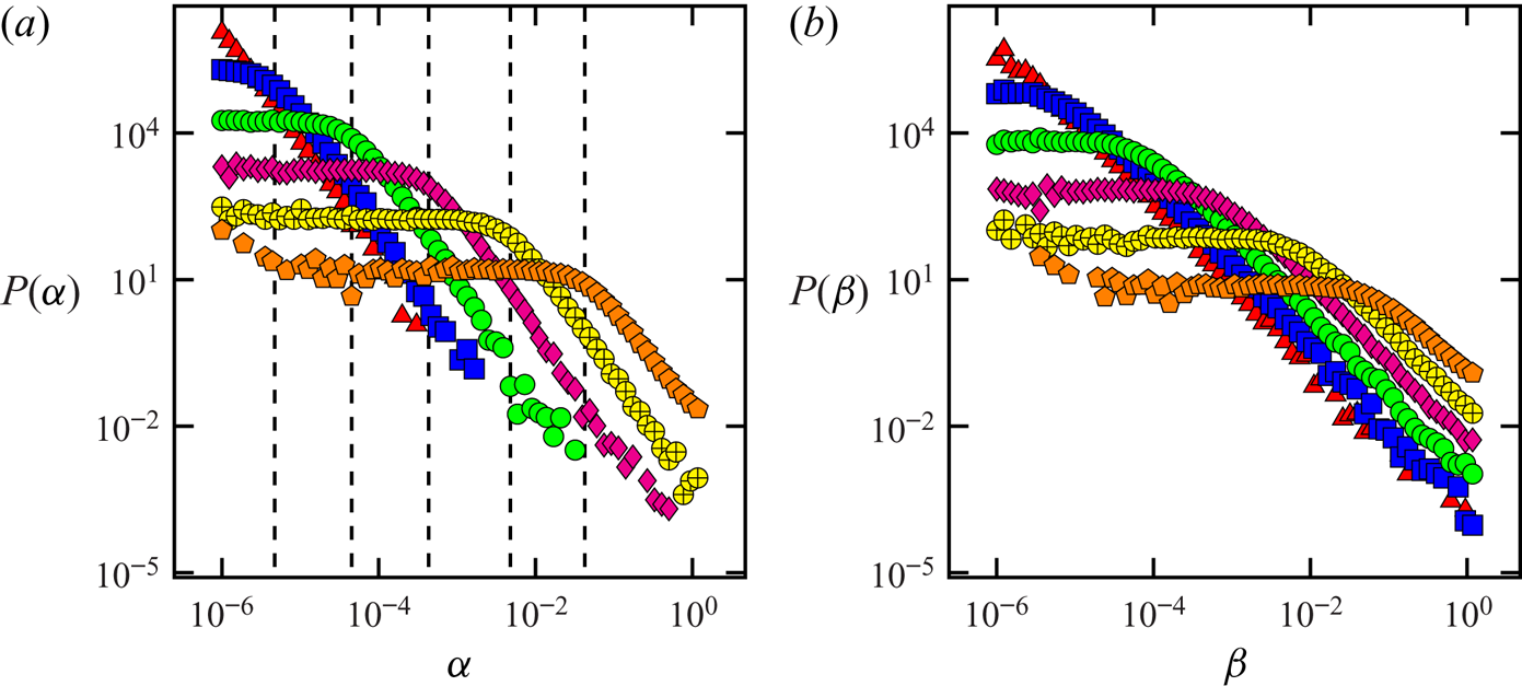
Distribution of alignment between  $\boldsymbol {n}(t)$ and
 $\hat {\boldsymbol {e}}_{{L}1}(t)$ near the channel centre at
 $z^+=180$. Shown are distributions of the Euler angles
 $\alpha$ and
 $\beta$, figure 1(a). (a) Distribution
 $P(\alpha )$. Red triangle, blue square, green circle, magenta diamond, yellow
 $\oplus$, orange pentagon symbols correspond to
 $\delta \Lambda =10^{-6},10^{-5},10^{-4},10^{-3},10^{-2},10^{-1}$, respectively (
 $\delta \Lambda = 1-\Lambda$). Vertical dashed lines show the cutoff angles where the power-law transitions to a plateau. (b) Same but for the distribution of
 $\beta$.

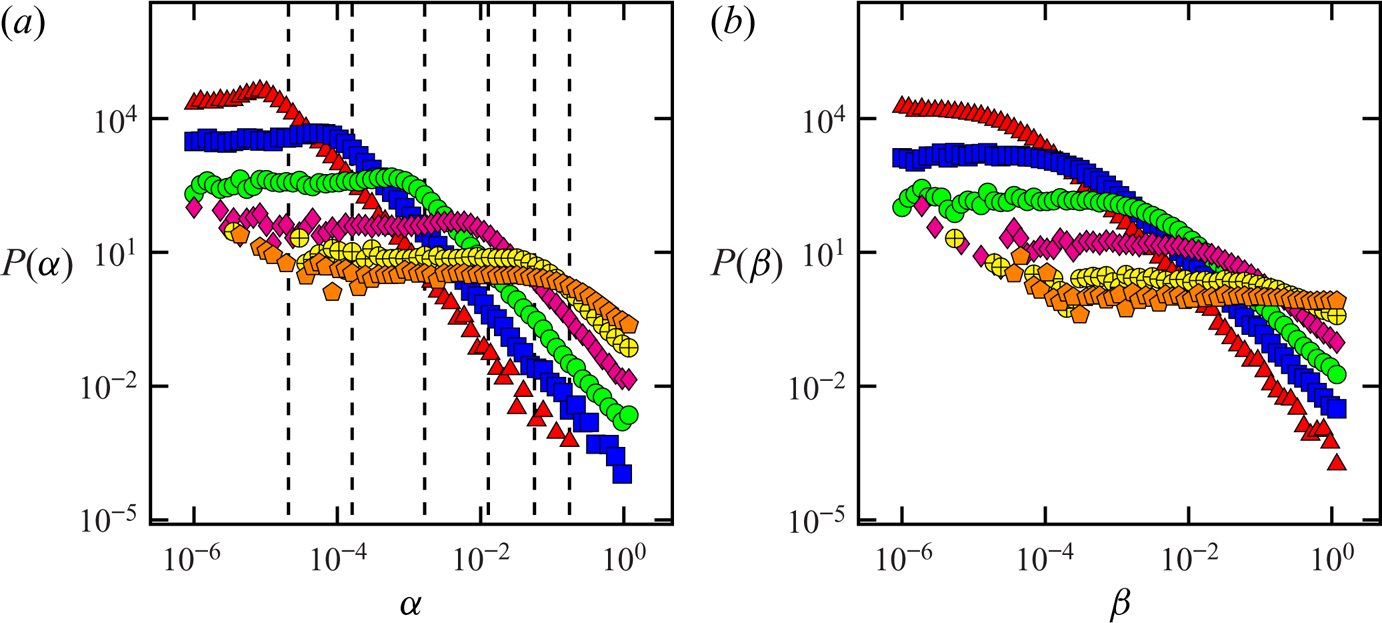
Distribution of alignment between  $\boldsymbol {n}(t)$ and
 $\hat {\boldsymbol {e}}_{{L}1}(t)$ near the channel wall at
 $z^+ = 4$. Shown are distributions of the Euler angles
 $\alpha$ and
 $\beta$, figure 1(a). (a) Distribution
 $P(\alpha )$. Red triangle, blue square, green circle, magenta diamond, yellow
 $\oplus$, orange pentagon symbols correspond to
 $\delta \Lambda =10^{-6},10^{-5},10^{-4},10^{-3},10^{-2},10^{-1}$, respectively (
 $\delta \Lambda = 1-\Lambda$). Vertical dashed lines show the cutoff angles where the power-law transitions to a plateau. (b) Same but for the distribution of
 $\beta$.

In figure 3 we plot DNS results for the distribution of the Euler angles  $\alpha$ and
 $\beta$ near the channel centre, at
 $z^+ = 180$. The figure shows distributions with power-law tails that are cut off at small angles by a plateau in the distribution. The narrow plateaus at small values of
 $\alpha$ and
 $\beta$ indicate that
 $\boldsymbol {n}(t)$ and
 $\hat {\boldsymbol {e}}_{{L}1}(t)$ align well most of the time. But we also see that the distributions have power-law tails, of the form
 $P(\alpha )\sim \alpha ^{\xi }$. For the largest values of
 $\Lambda$, close to unity, the exponent is close to
 $\xi =-2$, for both
 $\alpha$ and
 $\beta$. For
 $\Lambda =0.9$ the exponents are slightly smaller, although the power laws are not as clear cut for this value of
 $\Lambda$.
In figure 4 we plot DNS results for the distribution of the angles  $\alpha$ and
 $\beta$ near the channel wall at
 $z^+ = 4$, characterising the difference between the particle-symmetry vector
 $\boldsymbol {n}(t)$ and the Lagrangian stretching direction
 $\hat {\boldsymbol {e}}_{{L}1}(t)$ (figure 1a). The distributions look similar to the corresponding distributions near the channel centre. One difference is that distributions near the channel wall have a broader plateau than the corresponding distributions near the channel centre. A broader plateau in the distribution of relative angles corresponds to larger fluctuations in relative angles between
 $\boldsymbol {n}(t)$ and
 $\hat {\boldsymbol {e}}_{{L}1}(t)$. Both near the channel centre and the channel wall, the distributions show a power-law decay for large angles. This is an indication of large excursions in the relative angles between the orientation vector
 $\boldsymbol {n}(t)$ and
 $\hat {\boldsymbol {e}}_{{L}1}(t)$.
In summary, we find that near the channel centre rods with  $\Lambda$ close to unity tend to align with the Lagrangian stretching direction
 $\hat {\boldsymbol {e}}_{{L}1}(t)$. Zhao & Andersson (Reference Zhao and Andersson2016) found that very slender rods align with the Lagrangian stretching direction. Our results show that in fact the distribution of the relative angles between
 $\boldsymbol {n}(t)$ and
 $\hat {\boldsymbol {e}}_{{L}1}(t)$ has power-law tails that are cut off at small angles, giving rise to a plateau in the distribution. Figure 5 shows that the variance of the relative angles
 $\alpha , \beta$ near the channel centre is non-zero, indicating imperfect alignment between rod-like particles and the Lagrangian stretching direction. It is usually assumed that particles with aspect ratio larger than 10 (
 $\delta \Lambda \lesssim 0.02$) behave essentially like the Lagrangian stretching direction (Ni et al. Reference Ni, Ouelette and Voth2014). However, we show that near the channel centre, where turbulence is nearly homogeneous and isotropic, slender particles exhibit deviations away from the Lagrangian stretching direction. Near the channel wall, the alignment characteristics are similar: the distributions exhibit power-law tails at large relative angles and plateaus at small angles. However, the plateaus in the distributions near the channel wall are broader by an order of magnitude compared with the corresponding distributions near the centre. This indicates that typically the fluctuations of relative angles are larger near the wall than near the centre. Figure 5 shows how the variance of the relative angles
 $\alpha$ and
 $\beta$ decreases as the distance from the channel wall increases. The observed plateaus indicate random uncorrelated motion for small angles. We find that the mechanisms near the channel centre and the channel wall are different. Near the channel centre the distributions are a result of random fluctuations of the fluid-velocity gradients, whereas near the channel wall the dominant effects are the strong shear and the weak velocity-gradient fluctuations. In the next Section we discuss these observations and explain them using simple statistical models.
The variances  $\langle \alpha ^2 \rangle , \langle \beta ^2 \rangle$ of the angles
 $\alpha , \beta$ as a function of the wall normal distance
 $z^+$ for different values of
 $\delta \Lambda$. Red triangle, blue square, green circle, magenta diamond, yellow
 $\oplus$, orange pentagon symbols correspond to
 $\delta \Lambda =10^{-6},10^{-5},10^{-4},10^{-3},10^{-2},10^{-1}$, respectively (
 $\delta \Lambda = 1-\Lambda$).

4. Theory
4.1. Angular dynamics
The relative angular dynamics of spheroidal particles in channel flows can be understood by considering Jeffery's equation, (2.2), for the orientation vectors  $\boldsymbol {n}$ for
 $\Lambda =1$ and
 $\boldsymbol {n}_1$ for
 $\Lambda =1-\delta \Lambda$. Recall that the equation of motion of the Lagrangian stretching direction in the steady state is the same as an infinitely slender rod with
 $\Lambda =1$. In order to understand the relative angular dynamics, we first write the equation for the relative orientation,
 $\boldsymbol {\delta n} = \boldsymbol {n}-\boldsymbol {n}_1$. The equations of motion for
 $\boldsymbol {n}, \boldsymbol {\delta n}$, linearised in
 $\delta \boldsymbol {n}$, read
 \begin{gather} \dot{\boldsymbol{n}} = {\boldsymbol{A}} \boldsymbol{n} - (\boldsymbol{n} \boldsymbol{\cdot} {\boldsymbol{S}} \boldsymbol{n}) \boldsymbol{n} , \end{gather}
 \begin{gather}\dot{\boldsymbol{\delta n}} = - \delta \Lambda [{\boldsymbol{S}} \boldsymbol{n} - (\boldsymbol{n} \boldsymbol{\cdot} {\boldsymbol{S}} \boldsymbol{n}) \boldsymbol{n}] + [{\boldsymbol{A}}- (\boldsymbol{n} \boldsymbol{\cdot} {\boldsymbol{S}} \boldsymbol{n})] \boldsymbol{\delta n} - 2 (\boldsymbol{\delta n} \boldsymbol{\cdot} {\boldsymbol{S}} \boldsymbol{n}) \boldsymbol{n}. \end{gather}
Here  ${\boldsymbol{A}}$ is the fluid-velocity gradient matrix and
 ${\boldsymbol{S}}$ is the symmetric part of
 ${\boldsymbol{A}}$. The vectors
 $\boldsymbol {n}(t)$ and
 $\boldsymbol {\delta } \boldsymbol {n}(t)$ are computed along tracer particles and so experience fluctuating velocity-gradients along Lagrangian trajectories. Due to the space and time dependence of the velocity-gradients, (4.1) cannot be analytically integrated. In order to make progress, in the rest of this section we use a statistical model for the fluid-velocity gradients. In our statistical model we assume that the fluctuations of fluid velocity-gradients are much quicker than the time scale associated with the angular dynamics of rods (Zhao et al. Reference Zhao, Gustavsson, Ni, Kramel, Voth, Andersson and Mehlig2019). Such statistical models have led to important insights in the dynamics of small spherical particles in turbulence (Gustavsson et al. Reference Gustavsson, Berglund, Jonsson and Mehlig2016), as well as dynamics of relative angles between rods in turbulence (Zhao et al. Reference Zhao, Gustavsson, Ni, Kramel, Voth, Andersson and Mehlig2019). The flow near the centre of a turbulent channel flow resembles homogeneous, isotropic turbulence, where the time scales of angular dynamics of rods and fluctuations of fluid velocity-gradients are in fact very similar (Pumir & Wilkinson Reference Pumir and Wilkinson2011). Nevertheless, we expect our model to qualitatively describe the relative angular dynamics between slender rods and the Lagrangian stretching direction because the time scales of these two directions depend on the magnitude of the velocity gradients and the shape parameter
 $\Lambda$, not on the time scale of the fluid-velocity gradients. Near the channel wall, by contrast, we find that the angular dynamics of slender rods are much slower compared with the time scale of velocity-gradient fluctuations. This is because the large mean shear-rate near the channel wall leads to slow angular dynamics of rod-like particles. Thus, the statistical model near the channel wall turns out to be quantitatively accurate.
Equation (4.1) with rapidly fluctuating fluid-velocity gradients can be compared to multiplicative stochastic differential equations (Deutsch Reference Deutsch1994; Gustavsson et al. Reference Gustavsson, Mehlig and Wilkinson2015). The first term in (4.1b) is independent of  $\boldsymbol {\delta n}$ and the second term contains
 $\boldsymbol {\delta n}$ to the first power. These two terms are analogous to additive and multiplicative noises in stochastic differential equations because the fluid velocity-gradient matrix is an external noise for (4.1). Stochastic processes described by stochastic differential equations with multiplicative and additive noise are known to exhibit power-law tailed distributions, cut off by plateaus at small angles (Deutsch Reference Deutsch1994; Gustavsson et al. Reference Gustavsson, Mehlig and Wilkinson2015). In the rest of this section we show that this expectation is also true in our statistical models for relative angles.
4.1.1. Angular dynamics near the channel centre
To qualitatively explain why the distributions in figure 3 have power-law tails we consider a two-dimensional toy model for the angular dynamics (Zhao et al. Reference Zhao, Gustavsson, Ni, Kramel, Voth, Andersson and Mehlig2019). In two dimensions, the left Cauchy–Green tensor has two eigenvectors, the expanding eigenvector  $\hat {\boldsymbol {e}}_{{L}1}$ and the contracting eigenvector
 $\hat {\boldsymbol {e}}_{{L}3}$, but not the intermediate eigenvector
 $\hat {\boldsymbol {e}}_{{L}2}$. This means that the two-dimensional model may explain the dynamics of the angle
 $\alpha$ but not that of the angle
 $\beta$, see figure 1. Following Gustavsson & Mehlig (Reference Gustavsson and Mehlig2016) we model the homogeneous and isotropic fluid-velocity fluctuations as Gaussian random functions that are white in time, but have smooth spatial correlations. In two dimensions, (4.1) can be written in terms of two angles:
 $\phi$, the angle that the Lagrangian stretching direction makes with the
 $x$-axis in the channel coordinates, and
 $\alpha \approx |\boldsymbol {\delta n}|, |\boldsymbol {\delta n}| \ll 1$, the angular separation between the particle and the Lagrangian stretching direction. The angular separation between the Lagrangian stretching direction and the symmetry vector
 $\boldsymbol {n}$ of a particle with shape parameter
 $\Lambda = 1-\delta \Lambda$ is simply given by
 $\alpha = \phi (\Lambda =1)-\phi (\Lambda =1-\delta \Lambda )$. Here
 $\phi _{\Lambda }$ follows Jeffery's equation (2.2), for
 $\boldsymbol {n} = [\cos \phi _\Lambda , \sin \phi _\Lambda ]^{\textsf T}$. In the following we drop the subscript in
 $\phi _{\Lambda =1}$.
We start off by assuming the fluid velocity-gradient matrix to be a Gaussian random variable with time correlation  $\tau$. The dimensional parameters of the problem are the strength of velocity fluctuations,
 $u_0$, the correlation length
 $\eta$ and the correlation time
 $\tau$. Thus there are two relevant time scales, the correlation time
 $\tau$ and the advection time
 $\eta /u_0$. Out of these one can make one dimensionless parameter
 ${Ku} = u_0 \tau / \eta$ (Duncan et al. Reference Duncan, Mehlig, Östlund and Wilkinson2005). We non-dimensionalise the fluid-velocity gradient as
 ${\boldsymbol{A}} = ({{Ku}^2}/{\tau }) {\boldsymbol{A}}^\prime$ and the time as
 $t= ({\tau }/{{Ku}^2}) t^\prime$ and drop the primes in
 ${\boldsymbol{A}}, t$ in the following. Assuming tracelessness, and isotropy for the fluid gradient matrix
 ${\boldsymbol{A}}$, one finds that
 ${\boldsymbol{A}}$ has three independent components
 $O_{12}, S_{11},S_{12}$. Then for the variables
 $\phi$ and
 $\alpha$, (4.1) can be written as
 \begin{gather} \dot{\phi} = - O_{12} -\sin 2 \phi S_{11} + \cos 2 \phi S_{12} , \end{gather}
 \begin{gather}\dot{\alpha} = -(2 \alpha \cos 2 \phi + \delta \Lambda \sin 2 \phi) S_{11} + (- 2 \alpha \sin 2 \phi + \delta \Lambda \cos 2 \phi) S_{12}. \end{gather}
The white noise limit is taken as  ${Ku} \to 0$, which corresponds to assuming that the fluid velocity correlation time is the shortest time scale in the problem,
 $\tau \ll ({\eta }/{u_0})$. We find that the drift coefficients vanish. The diffusion coefficients are given by
 \begin{equation} \left.\begin{array}{c@{}} \mathcal{D}_{\alpha \phi} =\mathcal{D}_{\phi \alpha}= \dfrac{1}{2} \delta\Lambda , \\ \mathcal{D}_{\phi \phi} = \tfrac{3}{2}, \\ \mathcal{D}_{\alpha \alpha} = \dfrac{1}{2} (\delta \Lambda^2 + 4 \alpha^2). \end{array}\right\} \end{equation}
The stationary Fokker–Planck equation for the joint distribution  $P(\alpha ,\phi )$ is
 \begin{equation} \left[ \frac{3}{2}\frac{\partial^2}{\partial \phi^2} + \delta\Lambda \frac{\partial^2}{\partial \phi \ \partial \alpha} +\frac{\partial^2}{\partial \alpha^2} \frac{\delta\Lambda^2 + 4 \alpha^2}{2} \right]P(\alpha,\phi) = 0. \end{equation}
We obtain the marginal distribution  $P(\alpha )$ by integrating out
 $\phi$ from (4.4), requiring symmetry
 $P(\alpha ) = P(-\alpha )$, and that
 $P(\phi )$ is normalised to unity. The result is
 \begin{equation} P(\alpha) = \frac{\delta \Lambda }{[(\delta \Lambda) ^2+4 \alpha ^2 ] \tan ^{-1}\left(\dfrac{{\rm \pi} }{\delta \Lambda }\right)}. \end{equation}
Equation (4.5) captures the qualitative features mentioned before, namely the power-law form of the distribution and its cutoff at small angles, of the order of  $\delta \Lambda$. In the regime
 $\delta \Lambda \ll |\alpha | < {\rm \pi}/2$, where
 $\alpha$ is much larger than
 $\delta \Lambda$, the relative-angle distribution exhibits power-law tails. By contrast, in the regime
 $\alpha <\delta \Lambda$, the relative-angle distribution shows a plateau. Equation (4.2b) shows that at small angles
 $\alpha < \delta \Lambda$,
 $\dot {\alpha }$ is dominated by the additive term, which is the term independent of
 $\alpha$. This gives rise to the plateau in the distribution for
 $\alpha$, indicating random uncorrelated motion of
 $\phi _\Lambda$ and the Lagrangian stretching direction.
Using (4.5) we find that  $\langle \alpha ^2 \rangle =\frac 12 \delta \Lambda$ for
 $\delta \Lambda \ll {\rm \pi}$, so that the variance of the relative angle is proportional to the cutoff angle in the distribution of
 $\alpha$. The two-dimensional toy model predicts a linear dependence of the cutoff angle on
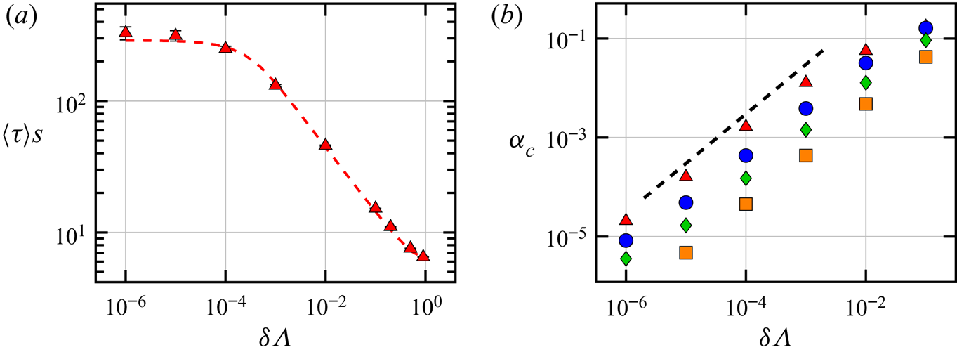
 $\delta \Lambda$. Figure 6(b) shows that the cutoff angle
 $\alpha _c$ depends linearly on
 $\delta \Lambda$ also in DNS of turbulent channel flow.
(a) Mean time between tumbles  $\langle \tau \rangle s$ as a function of
 $\delta \Lambda = 1-\Lambda$ for a set of trajectories in the layer
 $0<z^+ <10$,
 $s$ is the mean shear along the observed trajectories. Symbols correspond to simulation results, the dashed line corresponds to theory. (b) Here,
 $\alpha _{c}$ as a function of
 $\delta \Lambda$ for
 $z^+\sim 4$ (red triangles) and
 $z^+\sim 180$ (orange squares) where
 $\alpha _c$ describes the transition between the power law and the plateau in figure 3(a) in orange, and figure 4(a) in red. Blue circles and green diamonds correspond to
 $z^+ \sim 10, 20$, respectively. The black dashed line shows the reference slope
 $\delta \Lambda ^1$, as predicted by theory.

Geometrically, the power law in  $\alpha$ can be understood as a consequence of the fact that the Lagrangian stretching direction
 $e_{L1}(\boldsymbol {x}(t),t)$ acts as an attractor for the orientation field of particles with shape parameter
 $\Lambda$,
 $\phi _{\Lambda }(\boldsymbol {x}(t),t)$ along the same Lagrangian trajectory
 $\boldsymbol {x}(t)$. This clustering of orientations is analogous to spatial clustering of particles in turbulence in the advective limit (Gustavsson et al. Reference Gustavsson, Berglund, Jonsson and Mehlig2016; Meibohm et al. Reference Meibohm, Pistone, Gustavsson and Mehlig2017), and correlated random walks in the inertia free limit (Dubey et al. Reference Dubey, Meibohm, Gustavsson and Mehlig2018). Moreover, just as in the case of advected particles in one dimension, the power law in
 $\alpha$ is a result of purely diffusive dynamics with a diffusion coefficient proportional to
 $\alpha ^2$, leading to the same power-law exponent.
In the model the power-law exponent equals  $-2$, and it is independent of
 $\delta \Lambda$. The exponent is very nearly
 $-2$ for the DNS results but since the theoretical model we have considered is two-dimensional, we don't expect it to explain the exponent, but merely the mechanism. That the model agrees only qualitatively with DNS results is to be expected, the model neither describes the additional degree of freedom
 $\beta$, nor does it capture the persistent nature of the turbulent velocity-gradient fluctuations. But numerical simulations of a three-dimensional model show qualitatively similar results.
4.1.2. Angular dynamics near the channel wall
Near the channel wall the fluid-velocity gradient has a large shear component. Since the flow is anisotropic it is natural to express the angular dynamics in terms of the channel-fixed basis  $\hat {\boldsymbol {x}}$,
 $\hat {\boldsymbol {y}}$ and
 $\hat {\boldsymbol {z}}$ with the corresponding Euler angles
 $\theta$ and
 $\phi$, figure 1(b).
We consider a simple model for a spheroidal particle experiencing simple shear and additive noise. Turitsyn (Reference Turitsyn2007) used this model to study the angular dynamics of single polymers in a chaotic flow with mean shear. While Turitsyn (Reference Turitsyn2007) assumed  $\Lambda =1$, here we consider general values of the shape parameter
 $\Lambda$.
Decompose the fluid gradient matrix  ${\boldsymbol{A}}$ as a sum of the mean
 $\ \bar {\!\!{\boldsymbol{A}}}$ and the fluctuations
 ${\boldsymbol{A}}^\prime$ as
 ${\boldsymbol{A}} = \,\bar {\!\!{\boldsymbol{A}}} + {\boldsymbol{A}}^\prime$. The only non-zero component of
 $\ \bar {\!\!{\boldsymbol{A}}}$ is
 $\bar {A}_{xz} = s$ (Challabotla et al. Reference Challabotla, Zhao and Andersson2015). Jeffery's equation (2.2) for the angles
 $\phi ,\theta$ in terms of
 $s$ and
 ${\boldsymbol{A}}^\prime$ is given by
 \begin{gather} \dot{\phi} = -\frac{s}{2} (1 -\Lambda \cos 2 \phi) + \eta_\phi, \end{gather}
 \begin{gather}\dot{\theta} = -\Lambda \frac{s}{4} \sin 2 \phi \sin 2 \theta + \eta_\theta. \end{gather}
Here  $\eta _\phi$ and
 $\eta _\theta$ are fluctuating terms which in general depend on
 ${\boldsymbol{A}}^\prime$, the angles
 $\theta , \phi$ and the shape parameter
 $\Lambda$. In the vicinity of the channel wall the shear strength
 $s$ is much larger than the magnitude of fluctuations of the velocity-gradient matrix, and thus the particle spends long times close to
 $\phi = 0$. Since we have
 $\eta _\phi = A_{zx} + O(\phi )+ O(\theta )$ in the limit
 $\phi ,\theta \to 0$, one can approximate
 $\eta _\phi \approx A_{zx}$. Let the autocorrelation for
 $\eta _\phi$ be given by
 $\langle \eta _\phi (0)\eta _\phi (t)\rangle = C_0 \ f(|t|/\tau )$, so that
 $C_0$ quantifies the magnitude of the fluctuations and
 $\tau$ is the correlation time. Then, (4.6) has three time scales,
 $1/s, 1/\sqrt {C_0}$ and
 $\tau$. Near the wall the shear strength is much larger than the strength of the fluctuations,
 $s \gg \sqrt {C_0}$. This gives that the dynamics of
 $\phi$ is comprised of two regions, the deterministic fast region with time scale
 $1/s$ and the stochastic slow region with time scale
 $1/\sqrt {C_0}$. Observation of typical trajectories show that near the channel wall the fluctuations of
 $\eta _\phi$ are much faster than the time scale of the slow, stochastic
 $\phi$ dynamics. Thus we take the white noise limit as
 $\tau \sqrt {C_0} \to 0$, while holding
 $2 D= \int _{-\infty }^\infty \, \textrm {d} t \eta _\phi (0) \eta _\phi (t) \propto C_0 \tau$ constant.
Figure 2 appears to show a marked difference between the dynamics of the Lagrangian stretching direction and a rod-like particle with  $\Lambda = 0.9963$. In particular one observes that near the wall, the Lagrangian stretching direction seems to align along
 $\hat {\boldsymbol {x}}$ whereas
 $\Lambda =0.9963$ seems to tumble along the same trajectory. This can be explained by calculating the mean time between tumbles, defined as the average time taken by the particle to travel from
 $\phi =+{\rm \pi} /2$ to
 $\phi =-{\rm \pi} /2$, figure 6(a). A theoretical calculation using (4.6), see appendix A, shows good quantitative agreement with simulations. This is expected, considering that the parameter
 $\sqrt {C_0} \tau \sim 10^{-3}$ for the trajectory set used to obtain figure 6(a), so that the white noise limit is a good approximation.
Next we analyse the dynamics for  $\phi$. This is because the
 $\phi$ dynamics are independent of
 $\theta$, whereas the
 $\theta$ dynamics are slave to the process
 $\phi$.
Assuming  $\eta _\phi$ to be a Gaussian random variable, white in time, with the intensity of fluctuations
 $2 D = \int _{-\infty }^\infty \, \textrm {d} t \eta _\phi (0) \eta _\phi (t)$, Turitsyn (Reference Turitsyn2007) obtained the Fokker–Planck equation for the distribution of
 $\phi$,
 \begin{equation} \frac{\partial P(\phi,t)}{\partial t} = \frac{s}{2}\frac{\partial }{\partial \phi}[ (1 -\Lambda \cos 2 \phi)P(\phi,t)] + D \frac{\partial^2}{\partial \phi^2} P(\phi,t). \end{equation}
Equation (4.8) differs from (9) in Turitsyn (Reference Turitsyn2007) because we consider general values of  $\Lambda$ and not just
 $\Lambda =1$, and that the strength of fluctuations
 $D$ is defined slightly differently. Following Turitsyn (Reference Turitsyn2007), the steady-state distribution
 $P(\phi )$ is obtained as the time independent solution of (4.8),
 \begin{equation} P(\phi) = \mathcal{N} \int_0^{\rm \pi} \mathrm{d}x \exp-\frac{s}{2 D}(x -\Lambda \cos(2 \phi -x)\sin x). \end{equation}
Here one integration constant is determined by periodic boundary conditions,  $P({\rm \pi} /2) = P(-{\rm \pi} /2)$, and
 $\mathcal {N}$ is a normalisation constant which can be computed using
 $\int _{-{\rm \pi} /2}^{{\rm \pi} /2} \mathrm {d} \phi P(\phi ) =1$.
In order to understand how the relative angle between a slender rod and the Lagrangian stretching direction behaves, next we rewrite (4.1) for the relative angle,  $\delta \phi = \phi (\Lambda =1)-\phi (\Lambda =1-\delta \Lambda )$. The joint equations of motion for
 $\phi , \delta \phi$ up to the second order in
 $\delta \phi$ are given by,
 \begin{gather} \dot{\phi} = -\frac{s}{2} (1 -\cos 2 \phi) + \eta_\phi, \end{gather}
 \begin{gather}\dot{\delta\phi} = \frac{s}{2} \delta\Lambda \cos 2 \phi - (s \Lambda \sin 2\phi ) \delta\phi + (s \Lambda \cos 2\phi ) \delta\phi^2. \end{gather}
First assume  $\phi$ takes its mean value,
 $\phi _0 \approx ({\sqrt {{\rm \pi} }}/{\Gamma (1/6)})(\frac {3}{2})^{{1}/{3}} (D/s)^{{1}/{3}} \ll 1$. Then we have
 $\dot {\delta \phi } \approx ({s}/{2}) \delta \Lambda - (s \Lambda 2\phi _0 ) \delta \phi + (s \Lambda ) \delta \phi ^2$ to the first order in
 $\phi _0$. This equation has fixed points
 $\phi _0 \pm \phi _0 \sqrt {1-{\delta \Lambda }/{2\Lambda \phi _0^2}}$. For
 $\delta \Lambda \ll 2 \Lambda \phi _0^2$ there is a stable fixed point at
 $\delta \phi _c \approx {\delta \Lambda }/{4 \Lambda \phi _0}$ and an unstable fixed point at
 $2 \phi _0 - {\delta \Lambda }/{4 \Lambda \phi _0}$. At the end of this section, we argue that near the channel wall the distributions of
 $\alpha$ and
 $\beta$ get large contributions from the distributions of
 $\phi$ and
 $\theta$. Thus the stable fixed point explains the linear dependence of
 $\alpha _c$ on
 $\delta \Lambda$ near the channel wall, figure 6(b).
When  $\delta \Lambda = 2 \Lambda \phi _0^2$, the two fixed points merge to one, and for
 $\delta \Lambda > 2 \Lambda \phi _0^2$ there are no fixed points. For
 $\delta \Lambda > 2 \Lambda \phi _0^2$ the linear term in
 $\dot {\delta \phi }$ can be ignored. For the following we restrict ourselves to the regime
 $\delta \Lambda \ll 2 \Lambda \phi _0^2$ and ignore the
 $\delta \phi ^2$ term in (4.11):
 \begin{equation} \left.\begin{array}{c@{}} \dot{\phi} = -\dfrac{s}{2} (1 -\cos 2 \phi) + \eta_\phi, \\ \dot{\delta\phi} = \dfrac{s}{2} \delta\Lambda \cos 2 \phi - (s \Lambda \sin 2\phi ) \delta\phi. \end{array}\right\} \end{equation}
Chertkov et al. (Reference Chertkov, Kolokolov, Lebedev and Turitsyn2005) and Turitsyn (Reference Turitsyn2007) argued that the  $\theta$ distribution must have power-law tails in the case of a single polymer in a shear flow, with different power-law exponents arising from deterministic and stochastic
 $\phi$ dynamics, but were unable to analytically estimate the value of the exponent for the stochastic region. Similarly, we find that the
 $\delta \phi$ distribution exhibits two regimes corresponding to deterministic and stochastic
 $\phi$ dynamics, both of which lead to power-law tails for the distribution of
 $\delta \phi$ with different exponents. In addition we calculate the power-law exponent both in the deterministic and the stochastic region. The deterministic regime
 $|\phi | \gg \phi _0$ leads to a power-law exponent
 $-{3}/{2\Lambda }$ for
 $P(\delta \phi )$ and the stochastic regime
 $|\phi | \ll \phi _0$ with power law exponent
 $-1-{1}/{\Lambda }$ for
 $P(\delta \phi )$.
First consider the deterministic regime,  $|\phi | \gg \phi _0, \delta \phi > {\delta \Lambda }/{4 \Lambda \phi _0}$. In this regime the terms
 $\eta _\phi$ for
 $\dot {\phi }$ and
 $({s}/{2})\delta \Lambda \cos 2\phi$ for
 $\dot {\delta \phi }$ in (4.12) can be ignored. These equations can then be integrated to obtain
 $\delta \phi = C \sin ^{2\Lambda }\phi$ where
 $C$ is an integration constant. Using
 $P(\phi ) \sim \phi ^{-2}$, we obtain
 $P(\delta \phi ) \sim \delta \phi ^{-{3}/{2\Lambda }}$ by a change of variables.
Next consider the stochastic regime  $|\phi | \ll \phi _0, \delta \phi > {\delta \Lambda }/{4 \Lambda \phi _0}$. Then the term
 $({s}/{2})\delta \Lambda \cos 2\phi$ in (4.12) can be ignored. The steady-state Fokker–Planck equation reads,
 \begin{equation} \frac{\partial }{\partial \phi}\left[ \sin^2 \phi + \varepsilon^2 \frac{\partial}{\partial \phi}\right] P(\phi,\delta\phi) = - \Lambda \frac{\partial }{\partial \delta\phi}[\sin 2 \phi \delta\phi P(\phi,\delta\phi)], \end{equation}
where we have defined  $\varepsilon ^2 = {D}/{2s}$ in analogy with Meibohm et al. (Reference Meibohm, Pistone, Gustavsson and Mehlig2017). Numerics suggest that the joint probability factorises in the stochastic regime, so that
 $P(\phi , \delta \phi ) = f(\phi ) g(\delta \phi )$. We use separation of variables and obtain
 $g(\delta \phi ) \propto \delta \phi ^{-1-{\mu }/{\Lambda }}$. The equation for
 $f(\phi )$ is a generalised eigenvalue problem,
 \begin{equation} \frac{\partial }{\partial \phi}\left[ \sin^2 \phi + \varepsilon^2 \frac{\partial}{\partial \phi}\right] f(\phi) = \mu \sin 2\phi \ f(\phi). \end{equation}
It is possible to obtain an eigenvector corresponding to the eigenvalue  $\mu = 1$ for (4.14). The eigenvector has two undetermined integration constants which must be found by matching to the solution for large
 $\phi$ and normalisation. Thus we conclude that
 $g(\delta \phi ) = \delta \phi ^{-1-{1}/{\Lambda }}$ is a solution for the tail of the distribution of
 $\delta \phi$ in the regime
 $|\phi | \ll \phi _0, \delta \phi > {\delta \Lambda }/{4 \Lambda \phi _0}$. When
 $\Lambda \approx 1$ this would lead to a power law for
 $\delta \phi$ with exponent
 $\approx -2$. In figure 4(a) we have plotted the distribution for
 $\alpha$ which shows a power-law distribution for large
 $\alpha$, with exponent roughly
 $-2$. We argue next that since
 $\alpha$ must be closely related to
 $\delta \phi$ near the channel wall, the observed exponent
 $-2$ for
 $\alpha$ can be explained by our calculation for
 $\delta \phi$.
So far we have analysed the dynamics for the angle  $\phi$ in the channel frame for particles with shape parameter
 $\Lambda$. Since the Lagrangian stretching direction spends long times aligned with
 $\hat {\boldsymbol {x}}$, and the Lagrangian contracting direction spends long times aligned with
 $\hat {\boldsymbol {z}}$,
 $\alpha , \beta$ get large contributions from
 $\delta \phi , \delta \theta$, respectively. This means that near the channel wall one can use
 $\delta \phi$ and
 $\delta \theta$ as a proxy for understanding
 $\alpha$ and
 $\beta$, respectively. The precise calculation of the distributions of
 $\alpha , \beta$ is an open question left for future work.
In the presence of strong mean shear and weak velocity-gradient fluctuations we have shown that the width of the plateau in the distribution of relative angles scales linearly with  $\delta \Lambda$ and that the power-law exponent for the tail of the distribution is
 $-{3}/{2\Lambda }$ and
 $-1-{1}/{\Lambda }$ in the deterministic and stochastic regimes, respectively. Consider the relative angle in the case of constant shear without fluctuations. In the long time, the Lagrangian stretching direction reaches a steady state
 $\phi =0$, and thus the distribution of
 $\delta \phi$ has a plateau whose width scales as
 $\delta \Lambda ^{{1}/{2}}$ and an exponent
 $-2$ for the power-law tail of the distribution. Thus, the presence of weak fluctuations affects the relative angular dynamics sensitively and the observations cannot be explained in terms of just the strong mean shear.
5. Discussion
We have seen that the alignment of slender rods with the Lagrangian stretching direction in a channel flow depends on the distance of the particle from the channel wall, as well as the particle shape parameter  $\Lambda$. We found that the distributions of relative angles have power-law tails. A power-law tail implies that the relative angle exhibits large excursions. The power-law tails are cut off at small angles by a plateau. A plateau in the distribution implies that the relative angles are essentially uncorrelated at small angles. Near the channel centre the power law is a result of purely diffusive dynamics for the relative angle. Near the channel wall, by contrast, the power-law exponent is a result of the stochastic Lagrangian stretching direction dynamics and thus is a consequence of weak velocity-gradient fluctuations in addition to the strong mean shear. The plateau is broader near the channel wall than near the channel centre for particles with the same shape parameter. The width of the plateau near the channel wall depends on the ratio of the mean shear to the fluctuation strength of the velocity-gradient matrix element
 $A_{zx}$. Since the variance of the relative angle is described by the width of the plateau in the distribution, the large relative angles near the wall are a result of the mean shear strength being much larger than the velocity-gradient fluctuations. In general this implies that the particles show better alignment near the channel centre compared with near the channel wall.
A related important problem is understanding the relative angle between two particles as they approach each other. Since the velocity field is smooth at small scales, one might expect that as non-spherical particles approach each other, they tend to align in the same direction. However, Zhao et al. (Reference Zhao, Gustavsson, Ni, Kramel, Voth, Andersson and Mehlig2019) found that the relative angles between non-spherical particles close to each other show large excursions away from zero. This is quantified by the angular structure functions. The angular structure functions,  $\langle |\psi (r)|^p \rangle$, of spheroidal particles are a measure of the relative orientations of two particles with the same shape parameter
 $\Lambda$ at distance
 $r$. For homogeneous isotropic turbulence, the structure functions were studied by Zhao et al. (Reference Zhao, Gustavsson, Ni, Kramel, Voth, Andersson and Mehlig2019). The problem we have considered in this study, the relative angular orientation of a rod-like particle with respect to the Lagrangian stretching direction, is closely related to the structure functions.
Firstly, the problem of understanding the angular structure functions can be broken down into two parts: (a) understanding how a particle with shape parameter  $\Lambda$ aligns with respect to the Lagrangian stretching direction, which is a unique local reference vector; and (b) how the Lagrangian stretching directions at a spatial separation
 $r$ align with respect to each other. In this article we have tackled problem (a). Secondly, in two dimensions, the equations of motion for the angular structure functions, (A 1a)–(A 1c) in Zhao et al. (Reference Zhao, Gustavsson, Ni, Kramel, Voth, Andersson and Mehlig2019), exhibit striking similarities to the equations of motion for the problem discussed in this article (4.2a), the angular separation of a particle with shape parameter
 $\Lambda$ and the Lagrangian stretching direction.
In particular, the two equations for the angular separations have the same multiplicative term  $(\boldsymbol {n} \boldsymbol {\cdot } {\boldsymbol{S}}\boldsymbol {n})$. The two equations have different additive terms where the cutoff in (4.2a) is set by the small value
 $\delta \Lambda$ and the cutoff in the case of Zhao et al. (Reference Zhao, Gustavsson, Ni, Kramel, Voth, Andersson and Mehlig2019) is set by the small separation
 $\boldsymbol {R}$. In general, however, the required distribution of
 $\delta \psi$ is conditioned on small
 $\boldsymbol {R}$, which might in turn modify the distribution of the multiplicative term
 $\boldsymbol {n} \boldsymbol {\cdot } {\boldsymbol{S}} \boldsymbol {n}$. However, the calculation of this precise distribution remains an open problem.
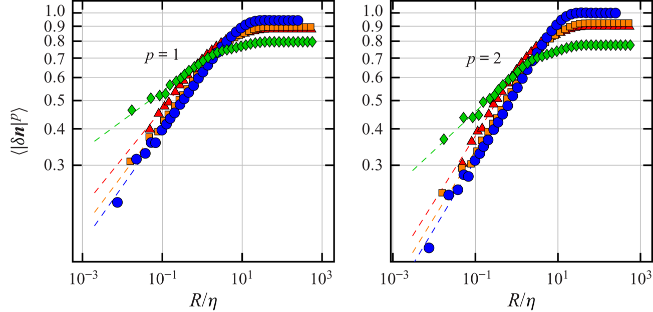
In a channel flow, one observes different scalings for the angular structure functions near the wall, in the viscous layer ( $z^+ < 5$), compared with the rest of the channel (figure 7). The smaller value of the scaling exponent near the wall implies larger relative angles between particles compared with the rest of the channel. Physically, we expect the mechanism causing larger relative angles between nearby particles near the channel wall to be related to the larger relative angles between the passive directors and the local Lagrangian stretching direction; however, the precise calculation is left for future work.
Angular structure functions  $S_p(r)$ plotted as a function of the particle separation
 $r$ for
 $\Lambda = 0.8$. Green diamonds, red triangles, orange squares, blue circles correspond to
 $z^+ \sim 0\text {--}5, 5\text {--}15, 15\text {--}25, 175\text {--}185,$ respectively. The left and right panels show the structure functions for
 $p=1$ and
 $p=2$, respectively. The dashed lines show power-law fits in the limit
 $R/\eta \to 0$. Observe that the scaling behaviour in the viscous layer
 $z^+<5$ is different from the scaling in the buffer layer, and near the centre of the channel.

6. Conclusions
We investigated the alignment of slender rod-like particles with the local Lagrangian stretching direction in a turbulent channel flow. Fluid flow close to the centre of a turbulent channel flow resembles homogeneous, isotropic turbulence, where it is usually assumed that rods with aspect ratio larger than 10 behave essentially like the Lagrangian stretching direction. Zhao & Andersson (Reference Zhao and Andersson2016) found that near the wall of a turbulent channel flow, slender rod-like particles tend to align with the Lagrangian stretching direction. We asked how this alignment depends on the particle shape parameter  $\Lambda$, and upon the distance of the particle from the channel wall. To this end we calculated the distribution of the relative angles between a particle with shape parameter
 $\Lambda = 1- \delta \Lambda$ and the Lagrangian stretching direction for different particle shape parameters and distances from the channel wall.
We found that the distribution of relative angles exhibits power-law tails at large angles cut off by plateaus at small angles both near the channel centre and the channel wall. At small angular separations the relative angles essentially perform uncorrelated random motion, leading to plateaus in the relative angle distributions. However, the relative angle exhibits large excursions away from alignment. These large excursions lead to power-law tails in the distributions of relative angles. The variance of the relative angle is closely related to the width of the plateau which depends on the distance of the particle from the channel wall as well as the shape parameter. We found that the width of the plateau is proportional to  $\delta \Lambda$ both near the channel centre and near the channel wall. However, the plateau near the channel wall is much broader than near the channel centre. Thus, we showed that the alignment of a slender rod with the Lagrangian stretching direction is stronger near the channel centre than near the channel wall. A non-zero variance of the distribution of relative angles indicates imperfect alignment, both near the channel centre and near the channel wall. Therefore, in contrast to usual expectations, our results indicate that a rod with a finite aspect ratio aligns imperfectly with the Lagrangian stretching direction. The misalignment increases with
 $\delta \Lambda$, and with decreasing distance to the channel wall.
We explained these observations using simple statistical models based on Jeffery's equation. Near the channel centre where turbulence is approximately homogeneous and isotropic, we used a two-dimensional toy model to qualitatively understand the distribution of relative angles. The two-dimensional toy model used to understand angular dynamics near the channel centre merely qualitatively explains the origin of plateaus and power-law tails in relative angle distributions using the white-noise approximation. In a turbulent channel flow, the orientational dynamics near the channel centre is three-dimensional, and the fluctuations of the velocity gradients are correlated in time. Taking into account time correlations and three-dimensional dynamics is an open question. Near the channel wall, where the turbulent velocity-gradient fluctuations are small and the mean shear-rate is large, we used the diffusion approximation for the three-dimensional dynamics to find excellent agreement with numerical simulations. The diffusion approximation works quantitatively near the channel wall because for very slender particles and for the Lagrangian stretching direction, the time scale of angular dynamics is much slower than the time scale of fluctuations of the velocity-gradient term  $A_{zx}$, which acts as additive noise. Our model near the channel wall predicts the distribution of
 $\delta \phi$, one relative angle in the laboratory frame. Using the fact that near the channel wall, the eigenvectors
 $\hat {\boldsymbol {e}}_{{L}1}, \hat {\boldsymbol {e}}_{{L}2}$ and
 $\hat {\boldsymbol {e}}_{{L}3}$ of the left Cauchy–Green tensor align well with
 $\hat {\boldsymbol {x}}, \hat {\boldsymbol {y}}$ and
 $\hat {\boldsymbol {z}}$, respectively, we argued that the distribution of
 $\delta \phi$ should closely resemble the distribution of
 $\alpha$. However, a direct analytical calculation of the relative angles
 $\alpha , \beta$ near the channel wall is a second open question. Finally, it is important to consider the range of shape parameters over which our models for relative angles are valid. The important assumption in our models both near the channel centre and channel wall is linearisation in the relative angles. Near the channel centre this approximation is valid up to
 $\delta \Lambda \sim O(10^{-1})$. By contrast, near the channel wall this happens when
 $\delta \Lambda \sim ({D}/{s})^{{2}/{3}}$, in our DNS this corresponds to
 $\delta \Lambda \sim 0.01$. Zhao & Andersson (Reference Zhao and Andersson2016) noted that rod-like particles with
 $\lambda =50$ (
 $\delta \Lambda \approx 10^{-4}$) tend to align well with the Lagrangian stretching direction, but
 $\lambda = 3$ (
 $\delta \Lambda = 0.2$) do not. Thus our model explains why the particle with
 $\delta \Lambda \approx 10^{-4}$ tends to align with the Lagrangian stretching direction, however, for
 $\delta \Lambda = 0.2$ our linearised model is not valid.
Mathematically, the fact that the distributions of relative angles are plateaus for small angles followed by power-law tails at large angles can be seen as a consequence of the general structure of the equations for relative orientations, (4.1b), which is analogous to that of a multicomponent stochastic process with additive and multiplicative noise (Kesten Reference Kesten1973; Deutsch Reference Deutsch1994). The additive term gives rise to the plateau whereas the multiplicative term gives rise to the power-law tail.
The plateau followed by a power-law tail in the distribution indicates that the particles spend most of the time at small relative angles, performing uncorrelated random motion, but rarely the relative angles show large excursions away from alignment. The power-law exponent for the tails of the relative angle distributions quantifies the frequency of the excursions. Near the channel centre, the power-law tails are a result of diffusive relative angular dynamics, with a diffusion coefficient that increases with increasing relative angle. This is analogous to the relative separation of advected particles in turbulence (Gustavsson et al. Reference Gustavsson, Berglund, Jonsson and Mehlig2016; Meibohm et al. Reference Meibohm, Pistone, Gustavsson and Mehlig2017). On the other hand, near the channel wall the power-law tails are a result of the weak velocity-gradient fluctuations and strong mean shear. This is because the dynamics of the relative angle between a very slender particle's orientation and the Lagrangian stretching direction depends sensitively on the dynamics of the Lagrangian stretching direction, which in turn depends on the strong mean shear and the weak fluctuations of the velocity-gradient matrix element  $A_{zx}$. The equation of motion of the Lagrangian stretching direction in the long-time limit is the same as that of a single infinitely slender polymer, whose dynamics in strong mean shear with weak isotropic fluctuations was analysed by Turitsyn (Reference Turitsyn2007).
The variance of the relative angle is given by the width of the plateau of the distribution. In our two-dimensional toy model, the width of the plateau is of the order of  $\delta \Lambda$ near the centre, but the model near the channel wall predicts a width of the order of
 $\delta \Lambda (s/D)^{1/3}$. Here
 $s$ is the strength of the mean shear and
 $D$ corresponds to the strength of fluctuations of the fluid velocity-gradient matrix element
 $A_{zx}$. Since
 $s/D \gg 1$, the plateau is broader near the channel wall, which explains the large relative angles between particle orientation and the Lagrangian stretching direction near the channel wall. Thus the large relative angles observed near the channel wall are a consequence of both the weak fluctuations of the fluid velocity-gradient element
 $A_{zx}$ and the strong mean shear. The importance of weak velocity-gradient fluctuations can be seen by the fact that in the absence of fluctuations, when the velocity-gradient matrix is constant with only a shear component, the width of the plateau scales as
 $\delta \Lambda ^{{1}/{2}}$ instead of
 $\delta \Lambda$, as observed.
The alignment of elongated particles along streamlines is important for the papermaking industry (Carlsson et al. Reference Carlsson, Söderberg and Lundell2010) as well as bacteria density profiles in inhomogeneous flows (Dehkharghani et al. Reference Dehkharghani, Waisbord, Dunkel and Guasto2019). Our results near the channel wall also explain how this orientation depends on the shape parameter of the particle. Another important question for the papermaking industry is the relative alignment of two nearby fibres. We have argued that this problem of understanding the relative angle distribution between two nearby elongated particles is related to the problem we have considered in the present study, and leave the calculation of the relative angle between nearby particles for arbitrary shape parameter for future work. Further, it would be interesting to analyse the relative angular dynamics between thin discs and the Lagrangian contracting direction. We expect the distributions of relative angles to also exhibit plateaus for small angles and power-law tails for large angles.
Acknowledgements
This work was supported in part by Vetenskapsrådet (grant number 2017-03865), by the grant ‘Bottlenecks for particle growth in turbulent aerosols’ from the Knut and Alice Wallenberg Foundation, Dnr. KAW 2014.0048, and by a collaboration grant from the joint China–Sweden mobility programme (NSFC-STINT) [grant numbers 11911530141 (China), CH2018-7737 (Sweden)]. Z.C. and L.Z. are grateful for the support of the Natural Science Foundation of China (grant numbers 11702158, 91752205) and the support from the Institute for Guo Qiang of Tsinghua University (grant number 2019GQG1012). A.D. would like to thank K. Gustavsson and J. Meibohm for helpful discussions. The authors Z.C. and A.D. contributed equally to this work.
Declaration of interests
The authors report no conflict of interest.
Appendix A. Time between subsequent tumbles
In order to explain the observed difference in tumbling characteristics for particles with  $\Lambda =1$ and
 $\Lambda =0.9963$ (figure 2), we calculate the mean time between subsequent tumbles as a function of the shape parameter
 $\Lambda$. Dehkharghani et al. (Reference Dehkharghani, Waisbord, Dunkel and Guasto2019) performed the same calculation for shape parameter
 $\Lambda =1$. Turitsyn (Reference Turitsyn2007) calculated the mean tumbling frequency and the distribution of times between subsequent tumbles, both for
 $\Lambda =1$. We define the time between subsequent tumbles as the time it takes for particles to travel from
 $\phi = +{\rm \pi} /2$ to
 $\phi = -{\rm \pi} /2$. To this end we start with (4.6) for
 $\phi$,
 \begin{equation} \dot{\phi} = -\frac{s}{2} (1 -\Lambda \cos 2 \phi) + \eta_\phi. \end{equation}
Here  $\eta _\phi$ is a Gaussian random variable, with
 $\langle \eta _\phi (t)\rangle =0, \langle \eta _\phi (t)\eta _\phi (t^\prime )\rangle = 2 D\delta (t-t^\prime )$. The corresponding Fokker–Planck equation can be written,
 \begin{gather} \frac{\partial P(\phi,t)}{\partial t} = \mathcal{L}_{FP} P(\phi,t), \end{gather}
 \begin{gather}\mathcal{L}_{FP}(\phi) = D \frac{\partial }{\partial \phi} \exp\left({-\frac{f(\phi)}{D}}\right) \frac{\partial }{\partial \phi} \exp\left({\frac{f(\phi)}{D}}\right), \end{gather}
where  $f(\phi ) = ({s}/{2}) (\phi -({\Lambda }/{2})\sin 2\phi )$. Then the mean exit time
 $T_1(\phi ^\prime )$ to exit the domain
 $\Omega = [{\rm \pi} /2,-{\rm \pi} /2)$ starting at
 $\phi ^\prime = {\rm \pi}/2$ can be calculated as follows. Let
 $P(\phi ,t \mid \phi ^\prime ,0)$ be the transition probability from
 $\phi ^\prime$ at time
 $0$ to
 $\phi$ at time
 $t$. The initial condition for the transition probability is
 $P(\phi ,0 \mid \phi ^\prime ,0) = \delta (\phi -\phi ^\prime )$. The probability that a trajectory starting at
 $\phi ^\prime \in \Omega$ at time
 $0$ is still in the domain
 $\Omega$ at time
 $t$ is
 $\int _\Omega \mathrm {d} \phi P(\phi ,t\mid \phi ^\prime ,0)$. This gives
 $1 - \int _\Omega \mathrm {d}\phi P(\phi ,t\mid \phi ^\prime ,0)$ as the cumulative probability that the first exit time is greater than
 $t$. This means that the probability density for the first exit time
 $\rho (t)$ is given by
 \begin{equation} \rho(t) = -\int_\Omega \mathrm{d}\phi \frac{\partial}{\partial t} P(\phi,t \mid \phi^\prime,0). \end{equation}
Thus one obtains the mean first exit time as,
 \begin{equation} T_1(\phi^\prime) = \int_0^\infty \mathrm{d}t \ t \rho(t) = -\int_\Omega \mathrm{d}\phi \int_0^\infty \mathrm{d}t \ t \frac{\partial}{\partial t} P(\phi,t\mid \phi^\prime,0). \end{equation}
Defining  $p_1(\phi ,\phi ^\prime ) = -\int _0^\infty \mathrm {d}t \ t ({\partial }/{\partial t}) P(\phi ,t\mid \phi ^\prime ,0)$, we obtain by integration by parts,
 $p_1(\phi ,\phi ^\prime ) = \int _0^\infty \mathrm {d}t \ P(\phi ,t\mid \phi ^\prime ,0)$. Then we have,
 \begin{equation} \mathcal{L}_{FP} p_1(\phi,\phi^\prime) = \int_0^\infty \mathrm{d}t \frac{\partial}{\partial t}\ P(\phi,t\mid \phi^\prime,0) = - \delta(\phi-\phi^\prime). \end{equation}
Thus  $p_1(\phi ,\phi ^\prime )$ satisfies the differential equation,
 \begin{equation} \mathcal{L}_{FP} p_1(\phi,\phi^\prime) = -\delta(\phi-\phi^\prime), \end{equation}
where  $p_1(\phi ,\phi ^\prime )$ must satisfy the same boundary conditions as
 $P(\phi ,t\mid \phi ^\prime ,0)$. For the calculation of the mean time it takes a trajectory starting at
 $\phi ^\prime = {\rm \pi}/2 - 0$ to travel to
 $-{\rm \pi} /2$ we use reflecting boundary condition at
 ${\rm \pi} /2$ and absorbing boundary condition at
 $-{\rm \pi} /2$. Then, (A 7) can be integrated to give,
 \begin{equation} p_1(\phi,{\rm \pi}/2-0) = - \frac{1}{D} \exp\left(-\frac{f(\phi)}{D}\right) \int_{-{\rm \pi}/2}^\phi\, \textrm{d} y \exp\left(\frac{f(\phi)}{D}\right) \int_{{\rm \pi}/2}^y \mathrm{d}z \delta(z-{\rm \pi}/2 + 0). \end{equation}
This gives for the mean time between tumbles,
 \begin{align} T_1({\rm \pi}/2-0) &= \int_{{\rm \pi}/2}^{-{\rm \pi}/2} \mathrm{d}\phi \ p_1(\phi,{\rm \pi}/2-0)\nonumber\\ &= \frac{1}{D} \int_{-{\rm \pi}/2}^{{\rm \pi}/2} \mathrm{d}\phi \exp\left(-\frac{f(\phi)}{D}\right) \int_{-{\rm \pi}/2}^\phi \mathrm{d}y \exp\left(\frac{f(y)}{D}\right). \end{align}
The corresponding equation in Dehkharghani et al. (Reference Dehkharghani, Waisbord, Dunkel and Guasto2019) is SI appendix, (19), with  $\Lambda =1$ and different boundary conditions. We further simplify this expression and obtain the asymptotics in the limit of small and large
 $\delta \Lambda$. Physically this corresponds to the transition in the shape parameter where the additive noise
 $\eta _\phi$ is no longer important. We obtain,
 \begin{equation} T_1 = \frac{1}{D} \int_{-{\rm \pi}/2}^{{\rm \pi}/2} \mathrm{d}\phi \int_{-{\rm \pi}/2-\phi}^0 \mathrm{d}y \exp\left(\frac{s}{2D}(y- \Lambda \cos (y+2\phi) \sin y)\right), \end{equation}
when  ${s}/{D} \gg 1$, the inner integral gets a large contribution near
 $y=0$, and decays quickly away from
 $y=0$, therefore we replace the lower limit in the inner integral by
 $-\infty$, then one can perform the integral over
 $\phi$ to obtain
 \begin{align} T_1 &= \frac{\rm \pi}{D} \int_{-\infty}^0 \mathrm{d}y \exp\left(\frac{s}{2D}y + \log I_0\left( \frac{s}{2 D} \Lambda \sin y\right)\right), \end{align}
 \begin{align} & = \frac{\rm \pi}{D} \int_{0}^\infty \mathrm{d}y \exp\left(-\frac{s}{2D}y + \log I_0\left( \frac{s}{2 D}\Lambda \sin y\right)\right), \end{align}
where we have changed integration variables  $y \to -y$, and
 $I_0(z)$ is the modified Bessel function. Next we use the asymptotic expansion of the modified Bessel function for large argument,
 $\log I_0(z) \sim z -\frac {1}{2}\log (2 {\rm \pi}z)$ to obtain
 \begin{equation} T_1 = \frac{\rm \pi}{D} \int_{0}^\infty \mathrm{d}y \exp\left(-\frac{s}{2D}y + \frac{s}{2 D}\Lambda \sin y -\frac{1}{2} \log\left( 2 {\rm \pi}\frac{s}{2 D}\Lambda \sin y\right)\right). \end{equation}
Using the Taylor expansion of the sine function we get,
 \begin{equation} T_1 = \frac{\rm \pi}{D} \int_{0}^\infty \mathrm{d}y \exp\left(-\frac{s}{2D}y + \frac{s}{2 D}\Lambda \left(y-\frac{y^3}{6}\right) -\frac{1}{2} \log\left( 2 {\rm \pi}\frac{s}{2 D}\Lambda y\right)\right). \end{equation}
Thus we have,
 \begin{equation} T_1 = \frac{\sqrt{\rm \pi} 12^{{1}/{6}}}{D} \left(\frac{D}{s \Lambda}\right)^{{2}/{3}} \int_{0}^\infty \mathrm{d}y \frac{1}{\sqrt{y}} \exp\left(- \left( \frac{3}{2}\right)^{{1}/{3}}\left(\frac{s}{D}\right)^{{2}/{3}} \frac{\delta\Lambda}{\Lambda^{1/3}} y - y^3 \right). \end{equation}
The behaviour of the integrand changes depending on the magnitude of the coefficient of  $y$ in the integrand. In the limit
 $\delta \Lambda \to 0$ the linear term can be neglected and the result is
 \begin{equation} T_1 = \frac{\sqrt{\rm \pi}2^{{4}/{3}} 3^{{1}/{6}} \Gamma(\tfrac{7}{6})}{D} \left(\frac{D}{s}\right)^{{2}/{3}}. \end{equation}
On the other hand when  $\delta \Lambda \gg ({D}/{s})^{{2}/{3}}$, the linear term dominates over the cubic term, and the result is
 \begin{equation} T_1 = \frac{\sqrt{2} {\rm \pi}}{s} \delta\Lambda^{-{1}/{2}}, \end{equation}
as predicted by Jeffery's theory.