Ever since the British and others were struck by American technology exhibits at the Crystal Palace Exhibition in 1851, it has been natural to give American education much of the credit for this country's advances in knowledge and its prosperity. Scholars have shown that by 1850 the Americans had roughly caught up with Prussia, the earlier leader, in the share of GDP devoted to education and also in enrollments.Footnote 1 The enrollment leadership relative to other countries came much earlier in mass primary education than in higher education. The Americans were also leaders in raising public tax money to supplement the traditional reliance on private tuition.
As Claudia Goldin and Lawrence F. Katz have emphasized, the movement was largely decentralized and spontaneous.Footnote 2 Americans at the grass-roots level often developed their primary schools some decades before help arrived from above, and they did it largely by voting to tax themselves. How did education arise so soon and so spontaneously in a country that resembled Russia in its rich opportunities in agriculture, forestry, and mining? Those nonspecialists who think of America's birth as antigovernment and antitax may also be puzzled by the willingness of early Americans to lead the world in shifting from private tuition toward taxes for primary schools.
Fortunately, specialists in the history of American education have advanced our understanding of these developments and the likely forces behind them. We know that the rise of primary schooling antedated the campaigns for state school systems led by Horace Mann, Henry Barnard, and Calvin Wiley.Footnote 3 Some of these forces have looked stronger than others, according to the careful analysis of Massachusetts experience by Carl Kaestle and Maris Vinovskis.Footnote 4 One other strand of scholarship has suggested for at least a century that something about American democracy and political voice favored education at public expense.Footnote 5
This article offers new evidence on how and why mass education spread so much sooner in some parts of North America than elsewhere, and tests competing ideas about underlying causes. Our analysis stresses the roles of three forces. The rural North led the world in the building of schools, the hiring of teachers, and overall enrollments because (a) basic education was supplied more affordably there, (b) decentralized local governments had more autonomy there, and (c) political voice was spread more broadly within its communities.
THE PATTERNS TO BE EXPLAINED
Among nations in the mid-nineteenth century, the United States was already becoming a leader in several respects. The contrast best known to observers at the time showed up in enrollment rates.Footnote 6 By mid-century, white children in the United States were already enrolled for as much primary schooling as children in any country other than Prussia, and most of that instruction was delivered in what were called public or common schools. The extra enrollment did not mean crowded classrooms: The United States may have stood out even more in its supply of teachers than in the more publicized enrollment rates, as best we can judge from incomplete and not always comparable measures. As of 1850 this country's elementary and secondary schools had 2.7 teachers per hundred students in public schools and 2.9 per hundred in all schools. No other country except perhaps France seems to have matched this rate. The striking supply of American teachers may have partly reflected two features to be discussed shortly: the use of part-time seasonal teachers, and the greater feminization of American teaching.
Antebellum America's distinction in the numbers of pupils and teachers was attained with a less outstanding level of expenditure on the part of its parents and taxpayers. Whether or not the United States was a leader at mid-century depends on the measure and concept one prefers. If one measures tax and tuition effort by the share of income spent on primary education, this country would again appear to have shared the lead with Prussia, both in public and in private expenditures. Yet it did not stand out in the generosity of primary-school tax support per child as a percentage of the average income per adult. Although the United States was well ahead of Britain, it was not ahead of France, Belgium, or Germany. The United States had more children per adult than those European countries, especially France, so that our expenditures were not outstandingly generous on a per child basis.Footnote 7
Within the United States, states and regions differed greatly in their commitment to schooling. Table 1 identifies some of the striking spatial patterns revealed by the census snapshot of 1850. What emerges, and demands explanation, is a distinctive style of the rural North, which accounted for most of this nation's high rates of schooling. Specifically, the rural North had over 70 percent of the nation's students and over 70 percent of its teachers, both among public schools and among all schools combined—even though the relative expenditures on schools were not so concentrated there. The South spent more than the North per pupil, and the cities spent more than the rural areas per pupil, partly because the South and the cities supplied a higher quality education through academies and colleges. The regional contrast was driven by private expenditures, with not much contrast in public expenditures per pupil. Cities outspent the rural areas, per pupil, both in public money and in private money. Clearly, rural Northern pupils attracted the fewest dollars. So did rural Northern teachers. Yet the mirror image is just as striking: It was the rural North that had the most students and the most teachers, per student or per child of school age. When we count people rather than dollars, the rural North stood out among regions in the same way that the United States stood out among countries. The strongest contrast favoring the rural North is shown by the row reporting the number of teachers per 100 free children of primary-school age: The rural North had twice as many as any other area.
U.S. EDUCATION IN 1850, URBAN AND RURAL COUNTIES

Notes:
The 15 Northern states are CT, IL, IN, IA, ME, MA, MI, NH, NJ, NY, OH, PA, RI, VT, and WI. The 15 Southern states are AL, AR, DE, FL, GA, KY, LA, MD, MS, MO, NC, SC, TN, TX, and VA. The 14 Northern urban (over 2,500 population) counties were Middlesex and Suffolk, MA; Providence, RI; Essex, NJ; Albany, Erie, Monroe, Kings, New York, and Rensselaer in NY; Allegheny and Philadelphia in PA; Cook, IL; and Hamilton, OH. The six Southern urban counties were St. Louis, MO; Henrico, VA; New Orleans, LA; Charleston, SC; Jefferson, KY; and Baltimore, MD. All other counties are called rural here. The enrollments are “gross” enrollments, including all pupils of any age, not just in the age range at which the type of school is primarily targeted. Public expenditures here equal taxes and “public funds,” but not endowment income, which is harder to divide between public and private sources. For regional totals that separate out the endowments, see Go and Lindert, “Curious Dawn,” table 1. The data generally refer to the school year 1849/50. The enrollments are “gross” enrollments, including all pupils of any age, not just in the age range at which the type of school is primarily targeted. Public expenditures here equal taxes and “public funds,” but not endowment income, which is harder to divide between public and private sources. For regional totals that separate out the endowments, see Go and Lindert, “Curious Dawn,” table 1. The data generally refer to the school year 1849/50.
Source:
The ICPSR electronic compilation of the 1850 census, see Haines, “Historical, Demographic, Economic, and Social Data.”
The contours of early American schooling can be drawn only very roughly, because schooling was a fluid, diverse, and voluntary experience before the Civil War, in ways that complicate our measurements.Footnote 8 Students moved in and out of school on an irregular basis, blending work experience with further installments of school learning. They went to school more regularly in the winter and summer than in fall or spring, and responded to daily changes in work and weather. Children might begin their studies at the age of three or four, and might be resuming them past the age of 20, after long absences. Such student transience has probably inflated some of the enrollment and attendance rates for the United States, and probably also for other countries before the late nineteenth century. There was probably some double counting of students who attended the separate summer and winter session, especially when they went to different schools. Eclecticism also characterized the teaching and the financing of schools. Teacher credentials and the curriculum were not at all standardized. The primary and secondary levels were not sharply divided from each other, even in the more public common-school system, and unregulated academies and grammar schools played a major role.Footnote 9 The state and national data-collectors coped with this diversity by grouping schools into two broad categories, the first being “public” or “common schools” and the second consisting of academies and “private and select schools.” We shall follow the same rough but convenient distinction here.
Who paid for the schooling? The numbers for New York State reveal the kind of private-public mix suggested by qualitative accounts for all Northern states. Total demand for primary schooling advanced ahead of public supply, and venture schools and academies stepped in to fill the gap.Footnote 10Figure 1 shows the breakdown of public school funding given by the official reports on New York's common schools. Parents and other private sources paid more than half of the cost of their children's schooling up to 1838–1840, when the common schools got a fresh infusion of state and federal money. Of the public funds, more than half came from local taxes until mid-century.
PUBLIC AND PRIVATE SHARES OF COMMON SCHOOL FUNDING, NEW YORK STATE, 1796–1850

Thus the early mix of funds was a half-empty and half-full glass, both for New York and for the nation. One could reasonably emphasize the long persistence of private tuition. On the other hand, there are two reasons for emphasizing the public half of the glass: The Northern states were ahead of Europe and the South in the reliance on public money and publicly run schools, and eventually every country that has developed universal primary schooling has come to rely primarily on taxes.
THREE SOURCES OF NORTHERN AMERICAN LEADERSHIP IN PUBLIC SCHOOLING
If the emergence of high Northern levels of primary schooling should be dated somewhere in the early nineteenth century, we still need to know why some areas had so much demand for schooling, and why local politics supplied so much of it from property taxes. This section turns to broad evidence suggesting three reasons why the rural North America differed from Europe, from Northern cities, and from the South. A later section will exploit the variations within regions to test the power of the same ideas.
More Affordable Schooling
Common folk in the northern states had higher labor incomes than their counterparts in Western Europe and in the American South, and had a more abundant supply of female teachers. We present some evidence first on the real income differences, and then on the relative price of schooling.
Since parents in richer areas tend to be less credit constrained and can invest more in schooling, the high enrollments will seem less puzzling if ordinary Northerners earned as much as their counterparts in Western Europe and the South. That appears to have been the case, though showing it requires turning away from national income estimates toward real wage data for ordinary folk. A clear transatlantic contrast in real incomes appears if we turn to a comparison of real wages for common occupational groups. Schooling has always been held back most severely for parents at lower income levels, who have less creditworthiness and less ability to invest in their children for a distant return. Economists have consistently found that the social rate of return is higher for poorer countries than for rich, and higher for primary education than for tertiary (e.g., university) education.Footnote 11 Those in higher income ranks can afford to pay for schooling out of pocket or by borrowing. The poor, by contrast, often lack the ability to purchase any schooling at all. If poor white Americans were better off than the poor in other countries, they might have spontaneously demanded more education—even if the nation as a whole had a lower real GDP per capita than Britain or the Netherlands.
REAL WAGES OF WORKERS IN MASSACHUSETTS AND IN ENGLAND, 1780S–1850S
What we are now learning about real wages around the world suggests that North American white workers in standard occupations could indeed buy more of the basics of life than workers anywhere else. Figure 2 offers a simple first clue, by comparing the ability of three common kinds of workers to buy an eight-commodity bundle of consumer goods in Massachusetts versus England, the ostensible world leader in GDP per capita. For each of the three occupational comparisons, workers in Massachusetts could buy more of that bundle than their counterparts in England. Carpenters in Massachusetts could buy more than English building craftsmen, and Massachusetts common laborers could buy more than English laborers, whether they worked in the building trades or in agriculture. Nor is this contrast sensitive to the choice of weights in the eight-commodity bundle, since most of the commodities cost fewer days of labor each year in America than in Europe. The Massachusetts workers probably could also pay less for housing, though they presumably paid more for cloth. Workers who could afford more of most basic goods than workers anywhere else in the world would also have had a better chance to afford a few years of basic schooling for their children. Similarly, as a hint about North-South differences, between 1800 and 1860 farm workers in Massachusetts enjoyed nearly twice the ability to buy food with their daily wage as did farmers in western Virginia.Footnote 12 Our estimates may be sensitive to unknown mismatches between wholesale and retail prices, or between wage rates that don't treat payments in kind (e.g., board and fuel) consistently. Yet the estimated real wage advantages of Massachusetts over England or western Virginia are great enough to withstand refinement of the measures.
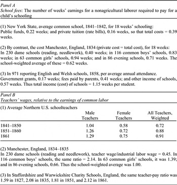
Even if laborers in the northern United States could afford more basic consumer goods than their counterparts in England or the South, their demand for schooling might have been no greater if they had to pay more for schools and for teachers than elsewhere. Yet the few available clues suggest that schooling, like basic consumer goods, was actually more affordable for those better-off workers in the northern states. So say the Anglo-American data contrasts in Table 2.Footnote 13 Contrasts in the costs of schooling are complicated, of course, by differences in school quality, length of school year, and the generosity of public subsidy. Nonetheless, schools seemed to cost a laborer fewer hours of pay in America than in England and Wales, both as a fee to be paid privately by parents and as a total annual cost per student. Let us compare the costs of educating a child for 18 weeks in 1840s New York and 1830s Manchester. The total private and public cost of that much primary schooling in New York in 1841/42 was only 0.39 weeks of common labor earnings, with the parents themselves paying less than half as much. By contrast, 18 weeks of primary schooling cost 0.62 weeks of common labor earnings in Manchester 1834, and more than that later. Table 2 offers other contrasts for various types of schools. In general, school was so much more affordable for workers in New York than in England that we should doubt that the whole difference was explained by school quality.
THE COST OF PRIMARY SCHOOLING AND TEACHERS, RELATIVE TO THE EARNINGS OF A COMMON LABORER IN THE UNITED STATES AND ENGLAND, 1830S–1850S

Sources:
School fees, Northern United States: New York State Superintendent for Common Schools, Annual Report to the State Legislature, divided by the average Northern laborer's wage, 1841, from Burgess (School Costs, p. 71). School fees in Manchester 1834: United Kingdom, House of Commons, “Education in England and Wales—Select Committee Report …” Sessional Papers, 1835 (465), vol. VII, pp. 111–112. Teachers’ wages and laborers’ wages in the Northern United States, 1841–1861: Burgess (School Costs, pp. 32–33, 71). We have weighted Burgess's separate wage rates for rural versus urban and male versus female teachers by the 1860 non-South employment weights in Perlman and Margo (Women's Work, p. 21). Teachers’ wages in Manchester 1834 are from the same pages of the 1835 Sessional Papers cited above. These are divided by the weekly earnings of nonagricultural common laborers used by Williamson (“Structure of Pay,” the 2L series). Teachers’ weekly wages in Staffordshire and Warwickshire Charity Schools are from Williamson (“Structure of Pay,” series 11H versus 2L). School fees for England and Wales 1858 are from United Kingdom, House of Commons, Report of the Commissioners … the State of Popular Education in England., Sessional Papers, 2794-I, 1861.
How could schooling cost fewer hours of parents’ labor in one country than in another, even when we are looking at the total costs shared by taxpayers, donors, and parents? Since school costs are dominated by teacher pay, one immediately wonders whether teachers were paid less in America than in England, relative to the earnings of common laborers. Panel B of Table 2 suggests an affirmative answer. Here again, as with fees, the comparison is complicated by differences in product, in this case the type of teacher. Still, it seems clear that on the average teachers were more affordable for common laborers and for parents of other occupations in New York than in England.
Teachers in the rural North might also have had lower relative pay than teachers in the South. For example, around 1853 Northern rural female teachers accepted lower monthly wages from common schools than teachers in North Carolina.Footnote 14 If deeper studies agree with these early hints, then rural Northern teachers may have been more affordable in the sense that paying for a teacher's services cost an ordinary Northern worker fewer days of his income than the cost faced by working families in England or the South.
One likely reason: The Northern states seem to have been world leaders in the feminization of teaching, a fact that may have made teachers less scarce relative to common laborers and other mostly male occupations.Footnote 15 Behind the Northern leadership in supplying female teachers lay an early lead in female literacy. We can now compare the signature literacy of brides (and bridegrooms) on both sides of the Atlantic from the seventeenth century on. Already by mid-eighteenth century, the young women of the Northern colonies were more literate than the young women of England, Scotland, and continental Europe, the leading possible competitors being women in Holland and Sweden.Footnote 16 Within the United States, females qualified to teach were more abundantly supplied in the lower-paying North, a fact reflected in the rise of Northern women as applicants for teaching jobs in North Carolina.Footnote 17 Opportunities for female employment were also more limited in Northern agriculture than in Southern agriculture, again pushing Northern women toward teaching as well as toward manufacturing.Footnote 18
Local Autonomy
By itself, greater affordability would only help to explain a higher private demand for education, and would not explain why taxes would be paid. In early settings, levying new taxes for schools was even more difficult than today, since the demand was still just emerging and public supply could be blocked by those who wanted labor to remain unskilled and abundant. An institutional feature that made it easier to launch public education on a limited scale was decentralization in voting on school issues. The more local the voting mechanisms, the greater the chance that an exceptionally high-demand local population could choose to tax itself, unblocked by opponents from other parts of the country.
Such decentralization of government was the second salient feature of the Northern states, relative both to Europe and to the American South. Schools were both financed and controlled more locally in the Northern states than elsewhere. The international contrast shows up in the revenue sources for schools in Europe and North America in the 1870s. The United States and Canada (along with Italy and the Netherlands) stood out by having schools paid for by local governments, rather than privately or by higher levels of government. England and Wales were the main bastion of reliance on private tuition.Footnote 19 The English and Welsh were trapped into centralization by Parliamentary rulings that put insurmountable barriers in the way of localities wanting to tax themselves for schools until a centralized fiscal solution was reached in 1891.Footnote 20
The South, like England, was more centralized than the Northern states. Historians have identified two Southern institutional tendencies that stood in the way of local school development: centralization of power throughout the region, and elitism in the laws governing membership in Southern legislatures. In both these institutional respects, the South resembled nineteenth-century England.
Throughout the South, state legislatures dominated, and seem to have appointed judges and county officials and even governors more often than in the North. County officials, in turn, retained power that might have devolved to townships.Footnote 21 The effect was much the same as in the case of Parliament's stifling local government taxes and services in nineteenth-century England: Localities had little freedom to raise their own taxes for schools or infrastructure within a larger polity that lacked their enthusiasm for such public goods.
The South also tended toward elitism in public office, though democracy was gaining over time and was stronger in the newer states. The most elitist laws of political representation were those in five states: North Carolina, South Carolina, pre-1851 Maryland, pre-1835 Georgia, and pre-1845 Louisiana all had stiff property requirements for serving in the legislature. Virginia had its own gerrymandered system of representation, explicitly designed to deny voice to the yeoman western counties and favor the slaveholding east in budgetary fights.Footnote 22
Voting and Voice
The third broad force that delivered more schooling in the American North than elsewhere was the breadth of political voice within each community. The likelihood of voting for taxes to pay for schooling depends on how political voice is distributed among the income ranks. Here too, ordinary white Americans had an advantage over common men in their European countries of origin: They had more political voice relative to local elites, and increasingly so over the first half-century of independence. The United States led Britain, France, and the rest of Europe, just as Stanley Engerman and Kenneth Sokoloff have emphasized that North Americans had more voting rights than Latin Americans.Footnote 23 The earlier suffrage of middling American white citizens seems to have accelerated the rise of public primary schooling, through mechanisms we will model and test in the next two sections.
Within each region, however, there were very different patterns of the franchise among counties. Even after states had repealed their property requirements for suffrage, most of them retained residency and citizenship requirements. Thus even in mid-century counties differed in how far suffrage extended down the ranks, much as if the earlier property restrictions emphasized by Engerman and Sokoloff were still in effect.Footnote 24 We argue that this should have mattered to schooling in theory, and that it did matter in practice. We next present a theory featuring a link from political voice to public schools, and later find that the predicted political influences indeed played a role in the North in the 1840s and 1850s.
MODELING THE POLITICAL SUPPLY AND PRIVATE DEMAND FOR SCHOOLING
Explaining the patterns in primary schooling means testing a model, one that simultaneously predicts how voting restrictions and other forces might have determined the levels of school attendance and of school financial support. This section sketches the assumptions and predictions of a simple public finance model presented more formally elsewhere.Footnote 25
The model must start from the schooling institutions of the rate-bill world before the 1850s. In this world, the local political process chose how many weeks of schooling to fund through local property taxes. Given that amount, parents would then decide whether to buy extra weeks’ worth of schooling by paying rate bills, or whether to buy schooling in private academies, where the share paid by taxes was lower and the quality of schooling generally higher. Accordingly, the model takes a form that predicts the supply and demand for both “common” (publicly administered) schools and all schools, including private academies. This allows the tests to shed light on the extent of “crowding out” of private by public education.
Within this institutional context, we model two standard kinds of optimizing behavior at once. First, the supply of tax-based schooling is chosen by the optimizing behavior of a decisive voter. Quality manifests itself as a share of the year that children spend in school, and an average class size. Second, each parental household, including that of a decisive voter, decides whether to enroll each child in school and whether to buy extra weeks of schooling by paying rate bills.Footnote 26 Their private demand is shaped by their incomes, by the supply of tax-based schooling, and by what the child could earn as a laborer instead of attending school.
The resulting equilibrium subsidy rates and attendance rates depend on the identity of the decisive voter. Note that the decisive voter is not just a classic “median voter,” for two reasons. First, if everybody voted, the decisive voter need not have a median property or education, because individual demand for tax-based schooling may be nonlinearly related to one's income or wealth ranking. Families with little or no property may have little taste for public schooling, especially since it costs them some income from child labor. They could ally with the tax-hating rich to defeat taxes and schools in the kind of “ends against the middle” redistributive politics featured in the work of Dennis Epple and Richard Romano.Footnote 27 Second, restrictions on political voice force the model to focus on a power-weighted decisive voice among those who have any say in the local politics of school finance. A highly restrictive access to voice might make the decisive voter somebody at the top of the property ranks, inclining him to feel the burden of a higher tax rate. As Engerman and Sokoloff and earlier authors have noted, the franchise tended to spread from the top down.Footnote 28 As property and tax requirements eased, the preferences of the decisive voter may have shifted non-linearly, first in favor of more school taxes and then away from them when the poorest voters gained a voice.
The combined model yields predicted coefficients for cross-sectional regressions on antebellum U.S. counties. For every educational outcome, be it the expenditures or the number of schools or teachers provided, or the enrollment response, the model predicts that the outcome depends positively on local income levels, positively on factors that should raise the perceived rate of private return to schooling, negatively on the direct and indirect cost of schooling, and positively on factors that should raise the political willingness to tax local property for schools. This political supply of tax support may depend nonlinearly on the share of white men who are franchised to vote.
DETERMINANTS OF SCHOOLING AT MID-CENTURY
We can exploit the diversity of conditions in antebellum communities to test our view of why some mustered more school support, and enrolled a greater share of children, than others. Fortunately, the national census of 1850 gathered data on schools, economic conditions, voting, religion, and other variables at the county level, and the 1840 Census reported some of the same variables.Footnote 29 Additional variables are available for the counties of New York State between 1820 and 1850. We use these data sets to test for the robustness of causal influences on education using the following county-level samples: (a) Northern, Southern, and all-state cross sections in 1850, (b) first differences between 1840 and 1850, (c) a New York State cross section having additional variables, and (d) first differences in the counties of New York State between 1821 and 1835, a time period experiencing shocks in voting rights. To save space, we shall present a table of results on enrollments alone, reporting elsewhere the determinants of public expenditure and the numbers of teachers and schools.Footnote 30
The econometric tests relate educational outcomes, such as enrollments, to a constrained set of independent variables that could be measured for 1850.

The dependent variables are educational outcomes per white child of the 5–14 age group, f(VoteRate) is a nonlinear function of the share of white men who vote, Slaves is the number of slaves per white man (South only), Children is the share of total population consisting of school-age children, OldMen is the share of men over the age of 40, ManuLabor is manufacturing labor as a share of white men over the age of 20, ManuInv is manufacturing capital per farm value, Migrants is the population share of migrants from other states, Foreign is the population share of the foreign born, FreeC is free coloreds per white, Geography i are four geography variables, Seating j are place-of-worship seating capacities for members of 23 separate religions as shares of total population, S k are fixed state effects, and e is the error term. The model from the previous sections predicts β5 β6 and β8 to be negative, but β9 to be positive.
The independent variables VoteRate and Slaves represent political supply. Having data on voting rates allows us to test two ideas at once. One is the common prediction that extending voting power to middle and lower income groups will monotonically raise taxes for schooling. The other is the Epple-Romano “ends again the middle” hypothesis. To test them both, the voting function needs to take a non-linear form. For the 1850 cross section of counties, we relate enrollments to a fourth-order polynomial in the voting rate:

Over most of the range of possible voting power, extending the vote to a greater share should raise the supply of taxes, schools, teachers, and government funds, and that the extra subsidies would make more parents enroll their children in school. Its effect could be linear or nonlinear. If the “ends against middle” hypothesis were correct, this function could curve downward as VoteRate approaches full 100 percent voting, since the poorest and least established men in the locality (the last to gain the vote) would tend, like the richest, to oppose taxes for schools. The fourth-order form allows us to test these possibilities, nesting the special case where the true effect of more voting is simply linear (β1 > 0, β2 = β3 = β4 = 0). Testing for the same possibly nonlinear voting effects on changes in schooling between 1840 and 1850 requires a slightly different approach. We have classified counties by the percentages of their men that voted in 1840, from the 0–10 percent range to the 90–100 percent range. Within each range, we measure the change in voting shares between the 1840 election and 1850. Thus the voting effect for first differences between 1840 and 1850 is allowed to test for the same potential nonlinearities as the 1850 cross section.
A second political supply variable is Slaves measurable in the 1850 census as the number of slaves per white man in the county. The model makes the conditional prediction that if Southern counties had budgetary autonomy, those with more slaves would have opposed paying taxes to impart skills to other white children. The remaining variables are generally demand-side control variables that either impose or relieve pressure on the budgets of households and of local governments.
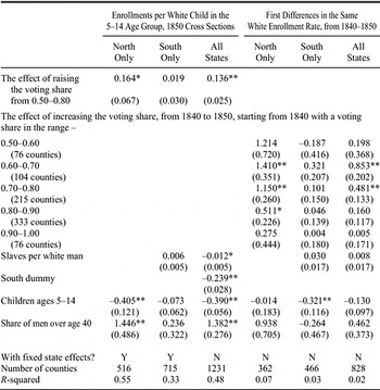
The regression results in Table 3 reveal some forces that made U.S. counties so different in their primary-school enrollments. The first three columns of results report on the 1850 cross section. To represent the right to vote in local fights over schools and taxes, we use the share of free men who actually voted for president, averaged over the 1848 and 1852 elections.Footnote 31 The impacts of the voting rate look strongly positive in the behavior of Northern U.S. counties, and for the nation as a whole. The first three columns of Table 3 show this by displaying how the slightly nonlinear function behaved over the heavily populated range between counties in which 50 percent of free men voted and counties in which 80 percent did so. As of 1850 households in the North's more heavily voting counties tended to enroll 19 percent more children in school.Footnote 32 There is a hint of an “ends against the middle” phenomenon. In those few counties where the share of men voting exceeded 80 percent, extra voting did not promote schooling, suggesting that the groups least often franchised gave no net support to taxes for schools, a point we develop further when looking at enrollment changes between 1840 and 1850. Still, the positive effect of voting on schooling prevailed over the dominant 50–80 percent range.
INFLUENCES ON ENROLLMENTS IN ALL SCHOOLS, U.S. COUNTIES IN 1840–1850

* = significant at the 5 percent level.
** = significant at the 1 percent level
Notes:
Robust standard errors of coefficients are in parentheses. The regression type is OLS. The hypothesis that all coefficients in the regression equal zero is rejected in an F-test at the 1 percent level for every equation. “Schools” refers to institutions providing pre-tertiary education. In the pre-graded era, most of these supplied the equivalent of primary education, with only a small share providing pre-primary or secondary education. The South consists of all states in the band running from Missouri through Kentucky, Virginia, Maryland, and Delaware, plus states further south, but excluding Texas. The North consists of all states north of this band. Children ages 5–14 = White children in this age band, per white male over 20 years of age. Share of men over 40 years of age = white males 40+ years of age/white males 20+ years of age, a measure that reflects the age of a community and its infrastructure. This demographic variable also tends to be a positive correlate of average wealth. Additional controls for 1850 = urban share, share foreign born, manufacturing labor share, manufacturing capital/farm capital, free coloreds per white, four geography variables, a South dummy (All-U.S. sample only), and seating capacities for members of 23 separate religions, as a share of total population. The 23 religious groups are defined by the 1850 census and by Michael Haines's ICPSR codebooks. The four geography variables are binaries for location on the Great Lakes, on the Atlantic or Gulf Coast, on the Mississippi, or on the Ohio River. Of these control variables for 1850, the data allowed us to first-difference only the urban share for 1840–1850. The equations for 1840–1850 first differences also contained similar voting variables starting from 0–0.50 voting shares in 1840, though these were rarities.
Sources:
Our edited data sets are available at http://www.econ.ucdavis.edu/graduate/sgo and http://econ.ucdavis.edu/faculty/fzlinder.
In fact, the positive impact of extra political voice on the supply of support for education was about the same for all schools as for public common schools. Extra voting, in other words, meant extra local tax support and extra enrollments that did not “crowd out” private support or private enrollments. So similar were the all-school versus public school effects of extra voting that we have omitted the public school regressions.
Within the South, the local voting rate had no clear effect on support per child or on enrollments within states. This null result held even though the shares of whites that voted were nearly as high in the South as in the North. The best explanation for the lack of a Southern county-level voting effect seems to be the institutional fact already noted: Southern policy was controlled by state legislatures, with little chance for a locality to tax itself for better schools. Within Southern states, the only significant county-level influence on educational outcomes was not voting, but the extent of local slave owning. At the state level, however, the more slave-holding states supplied fewer taxes for schools, and lowered enrollments as shown in Table 3.Footnote 33 So far, the regression clues suggest the sort of elitist imprint of slavery on education policy that past authors have described.Footnote 34
The control variables played less noteworthy roles, aside from the age shares shown in Table 3. Older populations generally supplied and demanded more schooling per child in the North. No such pattern is visible among Southern counties, where state legislatures controlled school spending.
Many observers have pointed to cities, and to their influx of foreigners, as forces that fostered support for schools, either as a way of solving social problems or as a response to higher private returns to schooling in the rising commercial and industrial sectors. Yet the quantitative geography of mid-century education patterns challenges us to re-interpret the demand and supply of urban schooling in the North. Unreported regressions agree with the simple raw averages shown in Table 1 that urbanization in particular had a very different impact in the North, relative to rural counties: (a) cities built fewer schools and hired fewer teachers per pupil, (b) they had slightly lower enrollments than did rural school districts, and (c) the presence of extra foreigners did not raise either enrollments or aid per child.Footnote 35 What was higher in large cities was not the provision of mass public education, but rather a greater emphasis on expensive education, involving a mixture of longer school years and fewer, more highly paid, teachers. True, the cities subsidized minimalist schools for the very poor, but this fell well short of universal schooling. The rural areas were ahead in the enrollment raceFootnote 36 and hired more teachers per hundred pupils.
ROBUSTNESS AND EXOGENEITY OF THE VOTING EFFECT
If voting rates so clearly differentiated Northern communities from each other, an immediate suspicion is that the voting rate may reflect something other than exogenous changes in voting rights. Perhaps the voting rates themselves were influenced by omitted variables that directly shaped educational outcomes, so that the voting rate is less of a cause, and more of a byproduct, than the cross-sectional 1850 analysis could reveal. Such influences common to both votes and schooling might be variables already included in Table 3, or might be such unobservables as local schooling efficiency (à la Charles M. Tiebout) or a local civic spirit.Footnote 37
To test the voting right hypothesis against such suspicions, we have run additional tests. In particular, the right-hand side of Table 3 uses county-level changes from 1840 to 1850 to test for the effects of changes in voting rights and voting rates on changes in enrollments, both in public schools and in all schools over that decade. This first-differences approach allowed us to purge all purely fixed differences between counties and between states. The first differences for 1840–1850 confirm that extra voting led to higher public school enrollments, especially for those counties starting in the 50–80 percent range back in 1840. For example, a Northern county that started with 70 percent voting in 1840 and had its voting share rise to 80 percent around 1850 would have 1.15 * 0.10 = 0.115 more enrollments, other things equal. That amounts to an increase of about 19 percent of the average Northern enrollment rate in 1840 (0.602). The pro-school effect was smaller when starting from more than 80 percent participation, consistent with the Epple-Romano hypothesis. And the decadal changes, like the cross-sectional differences, were similar whether one examines all schools or just public schools.
In addition to this first-differences test, we further tested for robustness by using the 1845 New York State data set that had county-level measures of franchised voting rights (as opposed to voting rates), measures of school attendance (as opposed to enrollments), and immigration from New England (as opposed to all other states). In every respect, the effect of voting rights on schooling was confirmed. We also exploited a natural experiment arising from New York's switch to near-universal manhood suffrage between 1821 and 1826. Property requirements for voting were repealed in 1821, and taxpaying requirements were repealed in 1826, leaving residency as the main requirement.Footnote 38 Over that four year span the share of adult men who obtained their formal right to vote jumped from 66 percent to 83 percent. In 1827/28 and again in 1832 the state legislature raised its common-school subsidies so much that by 1835 their real value per child age 5 to 16 was more than double that of the year 1820. Counties where the franchise was most extended tended to be those counties where common-school enrollments advanced fastest in this period. Thus the aftermath of New York's franchise liberalization of 1821–1826 also supports the findings based on regional or national census samples.Footnote 39
CONCLUSIONS AND AGENDA
It is much easier to explain the uneven early rise of public schooling in America if one focuses on the roles of affordability, local government autonomy, and the local distribution of political voice. All three of these influences are spotlighted by broad contrasts of the Northern states with the South and with Europe. One of the three, namely the distribution of political voice, also stands out in statistical tests of the determinants of support for funding schools. A wider voting franchise supplied more resources for schools at the county level, much as Engerman and Sokoloff found from their study of state-level correlations.Footnote 40
Our results invite a deeper exploration of the political economy of early American schooling. We especially invite studies of how the decision-making process really worked in town meetings and in state legislatures.Footnote 41