




1 Introduction
Many geophysical and man-made fluid flows are affected by the interaction between system rotation and turbulence (Greenspan Reference Greenspan1968; Boffetta & Ecke Reference Boffetta and Ecke2012). An idealized approach to study rotating turbulence consists in observing the evolution of an initial homogeneous isotropic flow in a non-inertial rotating frame of reference. This way, early experimental studies already revealed the main features of homogeneous rotating turbulence (e.g. Jacquin et al. Reference Jacquin, Leuchter, Cambon and Mathieu1990), although a few of them did not meet the condition for homogeneity (e.g. Ibbetson & Tritton Reference Ibbetson and Tritton1975; Hopfinger, Browand & Gagne Reference Hopfinger, Browand and Gagne1982). When the Rossby number ( $Ro$), i.e. the ratio of the rotational time scale and the turbulent time scale, was sufficiently small, it was observed that the energy dissipation rate
 $\unicode[STIX]{x1D700}_{\unicode[STIX]{x1D708}}$ is reduced with respect to the reference non-rotating isotropic case. Further, the typical cloud of isotropic eddies found in isotropic flows was strained, and grew in size towards an array of flow structures aligned with the axis of rotation (columnar eddies). These two features are the traits of rotating turbulence and have been observed and analysed in a number of recent experimental and numerical investigations – see e.g. Staplehurst, Davidson & Dalziel (Reference Staplehurst, Davidson and Dalziel2008), van Bokhoven et al. (Reference van Bokhoven, Clercx, van Heijst and Trieling2009), Mininni, Alexakis & Pouquet (Reference Mininni, Alexakis and Pouquet2009), Moisy et al. (Reference Moisy, Morize, Rabaud and Sommeria2011), Mininni, Rosenberg & Pouquet (Reference Mininni, Rosenberg and Pouquet2012) and Delache, Cambon & Godeferd (Reference Delache, Cambon and Godeferd2014), or Godeferd & Moisy (Reference Godeferd and Moisy2015) for a review. Yet, it remains poorly understood how they are quantitatively related.
For homogeneous isotropic turbulence, it is well accepted that the energy dissipation rate scales as  $\unicode[STIX]{x1D700}_{\unicode[STIX]{x1D708}}\sim u_{0}^{3}/l_{0}$, where
 $u_{0}$ and
 $l_{0}$ are an integral velocity scale and an integral length scale, respectively (Batchelor Reference Batchelor1953). This relation can be interpreted on the basis of phenomenological arguments as follows. Let us first assume that
 $\unicode[STIX]{x1D700}_{\unicode[STIX]{x1D708}}$ depends on an energy content, say
 $u_{0}^{2}$, and on a time scale
 $\unicode[STIX]{x1D70F}_{s}$ characteristic of the downscale energy transfer: the spectral transfer time. In homogeneous isotropic turbulence, the only time scale available to be taken as
 $\unicode[STIX]{x1D70F}_{s}$ is the time scale characteristic of the nonlinear triadic interactions,
 $\unicode[STIX]{x1D70F}_{nl}$. If we further assume that
 $\unicode[STIX]{x1D70F}_{nl}\sim l_{0}/u_{0}$, where
 $l_{0}$ is the typical size of the energy-containing eddies, the dissipation law for homogeneous isotropic turbulence can be recovered. But for systems in which other time scales are also relevant, as is the case of magnetohydrodynamics (MHD) or rotating turbulence,
 $\unicode[STIX]{x1D70F}_{s}$ might be different from
 $\unicode[STIX]{x1D70F}_{nl}$. Within the context of MHD, Kraichnan (Reference Kraichnan1965) considered that
 $\unicode[STIX]{x1D70F}_{s}$ is in fact composed of two time scales of opposing effects: the nonlinear time scale
 $\unicode[STIX]{x1D70F}_{nl}$, which can also be considered as the measure of how fast triple velocity correlations are built up, and the decorrelation time scale
 $\unicode[STIX]{x1D70F}_{3}$, which indicates how fast these correlations decay in time. Exploiting these ideas, he suggested that the energy flux (energy dissipation rate) was directly proportional to
 $\unicode[STIX]{x1D70F}_{3}$ and inversely proportional to
 $\unicode[STIX]{x1D70F}_{nl}$.
Following this line of thought, one alternative to relate the energy dissipation rate to the formation of columnar eddies in rotating turbulence is to find approximations for  $\unicode[STIX]{x1D70F}_{nl}$ and
 $\unicode[STIX]{x1D70F}_{3}$ that involve integral length scales and the rotation rate. However, this is not straightforward. First, owing to the fact that the distribution of energy is not isotropic, two distinct integral length scales in homogeneous rotating turbulence exist, i.e.
 $\ell _{0\,\bot }$ and
 $\ell _{0\,\Vert }$, which can be defined along the directions normal and parallel to the axis of rotation, respectively. Which one then is relevant to form
 $\unicode[STIX]{x1D70F}_{nl}$? Second, how does
 $\unicode[STIX]{x1D70F}_{3}$ depend on the time scale imposed by the background rotation, i.e.
 $\unicode[STIX]{x1D70F}_{\unicode[STIX]{x1D6FA}}=1/(2\unicode[STIX]{x1D6FA})$? In the literature, a few dissipation laws for homogeneous rotating turbulence have emerged from attempts to estimate the energy flux (Zhou Reference Zhou1995; Galtier Reference Galtier2003; Nazarenko & Schekochihin Reference Nazarenko and Schekochihin2011; Baqui & Davidson Reference Baqui and Davidson2015). Despite the efforts to account for the effects of rotation, the results available in the current literature regarding whether these laws generally hold or if they specifically apply to a Rossby-number range are inconclusive or even inconsistent.
Another problem, which is rather more technical, is the fact that the elongated columnar flow structures restrict the maximum observation time in direct numerical simulations (DNS) of rotating turbulence. Because simulations of homogeneous flows often consider periodic boundary conditions, a too small domain size with respect to the characteristic size of the living eddies can modulate the dynamics of the large scales and constrain their size. An obvious solution to circumvent this problem and avoid numerical artifacts is either to consider larger domains or to generate flow fields in which the characteristic eddy size is smaller than the domain size. For example, in the DNS by Baqui & Davidson (Reference Baqui and Davidson2015) the initial characteristic eddy size was 50 times smaller than the domain size. However, when  $Ro\ll 1$ this may still be insufficient and limit the simulation to a few eddy turnover times.
In view of these shortcomings, this study addresses the following two questions:
(i) What is the influence of the Rossby number in the growth rate of the columnar eddies, in the absence of confinement effects?
(ii) Can we approximate the energy dissipation rate in homogeneous rotating turbulence in a fashion similar to homogeneous isotropic turbulence, i.e. in terms of a velocity scale, an integral length scale and the rotation rate?
For this purpose, we consider the evolution of an initial homogeneous isotropic flow field in a rotating frame of reference. We conduct a systematic study that consists of 21 different rotation rates, thus covering a wide range of Rossby numbers. Our DNS are carried out in an elongated computational domain that is approximately 340 times larger than the initial characteristic size of the flow structures, and provides enough room for the columnar eddies to grow freely. All simulations are performed with a stochastic large-scale forcing that injects energy at a constant rate. The forcing scheme is three-dimensional, isotropic and at all times uncorrelated with the velocity field. To the best of our knowledge, the present database is unprecedented.
This work is organized as follows. In § 2, the governing equations and the numerical method is detailed together with a description of the simulations and their physical parameters. The influence of the Rossby number in the growth rate of the columnar eddies is investigated in § 3, and approximations for the energy dissipation rate are finally offered in § 4.
2 Numerical set-up
2.1 Governing equations and numerical method
We consider an incompressible fluid in a triply periodic rectangular cuboid of size  $2\unicode[STIX]{x03C0}{\mathcal{L}}_{1}\times 2\unicode[STIX]{x03C0}{\mathcal{L}}_{2}\times 2\unicode[STIX]{x03C0}{\mathcal{L}}_{3}$ that rotates around
 $\unicode[STIX]{x1D734}$. Fluid motion is assumed governed by the incompressible Navier–Stokes equations:
 $$\begin{eqnarray}\displaystyle & \unicode[STIX]{x1D735}\boldsymbol{\cdot }\boldsymbol{u}=0, & \displaystyle\end{eqnarray}$$
 $$\begin{eqnarray}\displaystyle & \displaystyle \frac{\unicode[STIX]{x2202}\boldsymbol{u}}{\unicode[STIX]{x2202}t}+(2\unicode[STIX]{x1D734}+\unicode[STIX]{x1D74E})\times \boldsymbol{u}=-\unicode[STIX]{x1D735}q+\unicode[STIX]{x1D708}\unicode[STIX]{x1D6FB}^{2}\boldsymbol{u}+\boldsymbol{f}. & \displaystyle\end{eqnarray}$$
Here,  $\boldsymbol{u}$,
 $\unicode[STIX]{x1D74E}$ and
 $\boldsymbol{f}$ are the velocity, the vorticity and an external force, respectively. Time is denoted by
 $t$, the reduced pressure, into which the centrifugal force is incorporated, is given by
 $q$, and
 $\unicode[STIX]{x1D708}$ denotes the kinematic viscosity of the fluid. The rotation vector
 $\unicode[STIX]{x1D734}$ is chosen to be aligned with the 3-direction, i.e.
 $\unicode[STIX]{x1D734}=(0,0,\unicode[STIX]{x1D6FA})$, where
 $\unicode[STIX]{x1D6FA}$ is the rotation rate. The horizontal dimensions of the rectangular cuboid (normal to the axis of rotation) are equal,
 ${\mathcal{L}}_{\bot }={\mathcal{L}}_{1}={\mathcal{L}}_{2}=1$, whereas the vertical extension (parallel to the axis of rotation) is by a factor of eight larger than the horizontal dimensions, i.e.
 ${\mathcal{L}}_{\Vert }={\mathcal{L}}_{3}=8$.
The numerical method is essentially the same as in Pestana & Hickel (Reference Pestana and Hickel2019b). Equations (2.1) and (2.2) are solved by a dealiased Fourier pseudo-spectral method (2/3 rule), where the spatial gradients are computed with the aid of fast Fourier transforms (Pekurovsky Reference Pekurovsky2012), and the time stepper employs exact integration of the viscous and Coriolis forces (Rogallo Reference Rogallo1977; Morinishi, Nakabayashi & Ren Reference Morinishi, Nakabayashi and Ren2001) together with a third-order low-storage Runge–Kutta scheme for the nonlinear terms. The number of degrees of freedom is  $N_{p}=768^{2}\times 6144$, which has been increased according to the extended domain size to resolve all scales of motion. The smallest and largest resolved wavenumbers per direction are
 $\unicode[STIX]{x1D705}_{min,i}=1/{\mathcal{L}}_{i}$ and
 $\unicode[STIX]{x1D705}_{max,i}=N_{p,i}/(3{\mathcal{L}}_{i})$, respectively, where the index
 $i=\{1,2,3\}$ denotes the different directions.
In all the simulations considered in this study, energy is injected through the external force  $\boldsymbol{f}$ on right-hand side of (2.2). The forcing scheme is designed as proposed in Alvelius (Reference Alvelius1999); the force spectrum
 $F(\unicode[STIX]{x1D705})$ is Gaussian with standard deviation
 $c=0.5$ and is centred around the forcing wavenumber
 $\unicode[STIX]{x1D705}_{f}$:
 $$\begin{eqnarray}F(\unicode[STIX]{x1D705})=A\exp (-(\unicode[STIX]{x1D705}-\unicode[STIX]{x1D705}_{f})^{2}/c).\end{eqnarray}$$
In (2.3), the prefactor  $A$, which controls the amplitude of
 $F(\unicode[STIX]{x1D705})$, can be determined a priori to the simulation and allow us to fix the power input
 $\unicode[STIX]{x1D700}_{I}$. This is only possible because this forcing scheme ensures that the force–velocity correlation is zero at all time instants. As a consequence, the injected power is an exclusive product of the force–force correlation, which is directly related to
 $F(\unicode[STIX]{x1D705})$. For more details about the forcing scheme and its design, please refer to Alvelius (Reference Alvelius1999).
2.2 Description of the simulations and physical parameters
To describe the considered physical problem, we are free to choose six control parameters. These form the set  $\{\unicode[STIX]{x1D705}_{f},\unicode[STIX]{x1D700}_{I},\unicode[STIX]{x1D708},{\mathcal{L}}_{\Vert },{\mathcal{L}}_{\bot },\unicode[STIX]{x1D6FA}\}$, which involves two physical units. Thus, a total of four non-dimensional numbers is sufficient to describe the numerical experiment. The governing non-dimensional numbers can be built by combination of the free control parameters. For instance, using
 $\unicode[STIX]{x1D705}_{f}$ and
 $\unicode[STIX]{x1D700}_{I}$ and assuming that the constant of proportionality is 1, we can construct the velocity scale
 $u_{f}=\unicode[STIX]{x1D700}_{I}^{1/3}\unicode[STIX]{x1D705}_{f}^{-1/3}$ and the time scale
 $\unicode[STIX]{x1D70F}_{f}=\unicode[STIX]{x1D705}_{f}^{-2/3}\unicode[STIX]{x1D700}_{I}^{-1/3}$. Additionally, a characteristic length scale can be taken as
 $\ell _{f}=1/\unicode[STIX]{x1D705}_{f}$. Hence, the Reynolds and the Rossby numbers are defined as
 $$\begin{eqnarray}Re_{\unicode[STIX]{x1D700}}=\frac{\unicode[STIX]{x1D700}_{I}^{1/3}\unicode[STIX]{x1D705}_{f}^{-4/3}}{\unicode[STIX]{x1D708}}\quad \text{and}\quad Ro_{\unicode[STIX]{x1D700}}=\frac{\unicode[STIX]{x1D705}_{f}^{2/3}\unicode[STIX]{x1D700}_{I}^{1/3}}{2\unicode[STIX]{x1D6FA}}.\end{eqnarray}$$
The two other governing non-dimensional numbers are formed by combining the forcing wavenumber with the geometric dimensions of the domain to yield  $\unicode[STIX]{x1D705}_{f}{\mathcal{L}}_{\bot }$ and
 $\unicode[STIX]{x1D705}_{f}{\mathcal{L}}_{\Vert }$. The four non-dimensional numbers,
 $\{Re_{\unicode[STIX]{x1D700}},Ro_{\unicode[STIX]{x1D700}},\unicode[STIX]{x1D705}_{f}{\mathcal{L}}_{\Vert },\unicode[STIX]{x1D705}_{f}{\mathcal{L}}_{\bot }\}$, whose definitions have been borrowed from Seshasayanan & Alexakis (Reference Seshasayanan and Alexakis2018), form the parameter space henceforth used to characterize the simulations performed in this study. Note, however, that this set of non-dimensional parameters is not unique. For instance, one may combine
 $Re_{\unicode[STIX]{x1D700}}$ and
 $Ro_{\unicode[STIX]{x1D700}}$ to form the microscale Rossby number
 $Ro_{\unicode[STIX]{x1D706}}=Re_{\unicode[STIX]{x1D700}}^{1/2}Ro_{\unicode[STIX]{x1D700}}$, which represents the ratio of rotation and Kolmogorov time scales, or express the geometric dimensions in terms of the domain aspect ratio
 $A_{r}={\mathcal{L}}_{\Vert }/{\mathcal{L}}_{\bot }$.
Another important parameter is the Zeman wavenumber  $\unicode[STIX]{x1D705}_{\unicode[STIX]{x1D6FA}}=(\unicode[STIX]{x1D6FA}^{3}/\unicode[STIX]{x1D700}_{I})^{1/2}$, which indicates the wavenumber range for which rotational effects are relevant (Zeman Reference Zeman1994; Delache et al. Reference Delache, Cambon and Godeferd2014). The Zeman wavenumber is also automatically set by fixing the aforementioned parameters as
 $Ro_{\unicode[STIX]{x1D700}}=(\unicode[STIX]{x1D705}_{f}/\unicode[STIX]{x1D705}_{\unicode[STIX]{x1D6FA}})^{2/3}/2$.
A posteriori, we can compute the usual physical parameters that describe the flow field. The box-averaged kinetic energy  $K$ is given by
 $\langle u_{i}u_{i}\rangle _{{\mathcal{L}}}/2$, where the operator
 $\langle \cdot \rangle _{{\mathcal{L}}}$ denotes volume averages, and the viscous dissipation rate is
 $\unicode[STIX]{x1D700}_{\unicode[STIX]{x1D708}}=2\unicode[STIX]{x1D708}\langle \unicode[STIX]{x1D61A}_{ij}\unicode[STIX]{x1D61A}_{ij}\rangle _{{\mathcal{L}}}$, where
 $\unicode[STIX]{x1D61A}_{ij}=(\unicode[STIX]{x2202}u_{i,j}+\unicode[STIX]{x2202}u_{j,i})/2$ is the strain-rate tensor. From
 $K$, we define the root-mean-square (r.m.s.) velocity
 $u^{\prime }=\sqrt{2K/3}$, which is used to define the large-eddy turnover time
 $T_{e}={u^{\prime }}^{2}/\unicode[STIX]{x1D700}_{I}$. The Taylor microscale is defined as in Pope (Reference Pope2000), i.e.
 $\unicode[STIX]{x1D706}=(15\unicode[STIX]{x1D708}{u^{\prime }}^{2}/\unicode[STIX]{x1D700}_{\unicode[STIX]{x1D708}})^{1/2}$. The Taylor-microscale Reynolds number is computed as
 $Re_{\unicode[STIX]{x1D706}}=u^{\prime }\unicode[STIX]{x1D706}/\unicode[STIX]{x1D708}$, and the Kolmogorov length scale is
 $\unicode[STIX]{x1D702}=(\unicode[STIX]{x1D708}^{3}/\unicode[STIX]{x1D700}_{\unicode[STIX]{x1D708}})^{1/4}$.
Last, we define the integral length scales along the directions normal and parallel to the axis of rotation. These are constructed from the two-point velocity correlation:
 $$\begin{eqnarray}R(\boldsymbol{r})=\frac{\langle u_{i}(\boldsymbol{x})u_{i}(\boldsymbol{x}+\boldsymbol{r})\rangle _{{\mathcal{L}}}}{\langle u_{i}(\boldsymbol{x})u_{i}(\boldsymbol{x})\rangle _{{\mathcal{L}}}},\end{eqnarray}$$
where  $\boldsymbol{r}=r_{i}\,\hat{\boldsymbol{e}}_{i}$ is an arbitrary position vector. We integrate (2.5) with
 $\boldsymbol{r}=r\,\hat{\boldsymbol{e}}_{r}$, as in spherical coordinates, or with
 $\boldsymbol{r}=r_{\bot }\hat{\boldsymbol{e}}_{\bot }$ and
 $\boldsymbol{r}=r_{\Vert }\hat{\boldsymbol{e}}_{\Vert }$, as in cylindrical coordinates, to obtain the integral length scales along the respective directions:
 $$\begin{eqnarray}\ell =\int _{0}^{\unicode[STIX]{x03C0}{\mathcal{L}}_{min}}R(r)\,\text{d}r,\quad \ell _{\bot }=\int _{0}^{\unicode[STIX]{x03C0}{\mathcal{L}}_{\bot }}R(r_{\bot })\,\text{d}r_{\bot }\quad \text{and}\quad \ell _{\Vert }=\int _{0}^{\unicode[STIX]{x03C0}{\mathcal{L}}_{\Vert }}R(r_{\Vert })\,\text{d}r_{\Vert }.\end{eqnarray}$$
In (2.6),  ${\mathcal{L}}_{min}$ is taken as
 $\min ({\mathcal{L}}_{\Vert },{\mathcal{L}}_{\bot })$ in the limit of the integral that defines
 $\ell$. To represent quantities from the initial and isotropic flow field, we use the superscript iso, as in
 $\ell ^{iso}$.
2.2.1 Initial conditions
The initial conditions for the simulations with rotation are produced by injecting energy at constant rate  $\unicode[STIX]{x1D700}_{I}$ to a fluid that is initially at rest. The energy, which is injected at wavenumber
 $\unicode[STIX]{x1D705}_{f}=8$, is progressively distributed over a wider range of wavenumbers by the velocity triad interactions. When the energy cascade is built up, the box-averaged kinetic energy
 $K$ stops growing and a steady state is reached. The numerical resolution guarantees that at all times
 $\unicode[STIX]{x1D705}_{max}\unicode[STIX]{x1D702}\geqslant 1.5$, which is sufficient to resolve all scales of motion. The initial transient lasts for
 $20\unicode[STIX]{x1D70F}_{f}$ or, equivalently,
 $8.45T_{e}$, and afterwards statistics are collected for another
 $54\unicode[STIX]{x1D70F}_{f}$ (
 $22.84T_{e}$). For the fully developed field, we find that
 $Re_{\unicode[STIX]{x1D706}}\approx 68$, and that the relation
 $\ell ^{iso}=\ell _{\Vert }^{iso}=\ell _{\bot }^{iso}$ holds up to two decimal places. The latter suggests that the flow field is in fact isotropic.
Other statistics of the steady state match closely with typical values found in DNS of homogeneous isotropic turbulence. For instance, the skewness and flatness of the longitudinal velocity derivative  $\unicode[STIX]{x2202}u_{1}/\unicode[STIX]{x2202}x_{1}$ are -0.51 and 4.8, respectively, in agreement with Van Atta & Antonia (Reference Van Atta and Antonia1980) and Tang et al. (Reference Tang, Antonia, Djenidi, Danaila and Zhou2018). The energy dissipation rate
 $\unicode[STIX]{x1D700}_{\unicode[STIX]{x1D708}}$ at the steady state is well approximated by
 $\unicode[STIX]{x1D700}_{\unicode[STIX]{x1D708}}=C_{\unicode[STIX]{x1D700}}^{iso}({u^{\prime }}^{iso})^{3}/\ell ^{iso}$, where
 $C_{\unicode[STIX]{x1D700}}^{iso}\approx 0.35$ is the constant of proportionality. Note, however, that the value of this constant depends on how the two-point correlation in (2.5) is normalized. If we normalize it with
 $2u^{\prime 2}$, like in Kaneda et al. (Reference Kaneda, Ishihara, Yokokawa, Itakura and Uno2003), instead of
 $2K$, like in (2.5), a factor of 3/2 must be accounted for to yield
 $C_{\unicode[STIX]{x1D700}}^{iso}\approx 0.5$ in agreement with the literature; see Ishihara, Gotoh & Kaneda (Reference Ishihara, Gotoh and Kaneda2009) for a compilation of other numerical results.
In this study, the goal is not to achieve the highest possible Reynolds number for a given numerical resolution. Instead, we focus on maximizing the time for which large-scale eddies with typical size  $\ell ^{iso}$ can evolve unbounded, while still resolving all scales of motion. Therefore, apart from forcing at scales smaller than usual, we consider an elongated domain with
 $A_{r}=8$. As a result, the isotropic fields to which background rotation can be imposed are, in the vertical direction, approximately 340 times larger than
 $\ell ^{iso}$ and, in the normal direction,
 $2\unicode[STIX]{x03C0}{\mathcal{L}}_{\bot }/\ell ^{iso}\approx 40$. In figure 1, we show evidence of these aspects. Figure 1(a) confirms through the two-point velocity correlation along the normal and the parallel directions that the ratio of domain size to flow structures is indeed significantly larger in the vertical direction. The area below the curves equals
 $\ell _{\bot }^{iso}/(\unicode[STIX]{x03C0}{\mathcal{L}}_{\bot })$ and
 $\ell _{\Vert }^{iso}/(\unicode[STIX]{x03C0}{\mathcal{L}}_{\Vert })$, respectively. Alongside, figure 1(b) verifies that the velocity fields are isotropic, as the curves for the one-dimensional energy spectra along the normal and perpendicular directions overlap.
Two-point velocity correlations showing the ratio of domain size to characteristic size of the flow structures in the different directions, and one-dimensional energy spectra showing that the initial conditions are indeed isotropic. (a) Normal  $R(r_{\bot })$ (– – –) and parallel
 $R(r_{\Vert })$ (——, black) velocity two-point correlations. (b) Perpendicular and parallel one-dimensional energy spectra:
 $\unicode[STIX]{x1D6FC}=1$,
 $\unicode[STIX]{x1D6FD}=3$,
 $E_{11}(\unicode[STIX]{x1D705}_{3})$ (——, blue); and
 $\unicode[STIX]{x1D6FC}=3$,
 $\unicode[STIX]{x1D6FD}=1$,
 $E_{33}(\unicode[STIX]{x1D705}_{1})$ (○).

These features are also clearly visible in the flow-field visualization (see figure 2), where we show a subset of the computational domain with the flow structures visualized by the  $Q$-criterion of Hunt, Wray & Moin (Reference Hunt, Wray and Moin1988) and coloured by the normalized projection of the vorticity vector on the axis of rotation, i.e.
 $\unicode[STIX]{x1D74E}\boldsymbol{\cdot }\boldsymbol{e}_{\Vert }/\Vert \unicode[STIX]{x1D74E}\Vert$. Reinforcing the aforementioned results, we observe two main points in the isotropic field that is used as initial condition for the runs with rotation (figure 2a). First, the flow structures do not display any preferential sense of rotation, which is confirmed by the uniform distribution of the colours. Second, they are also isotropically arranged and therefore not aligned along any preferential direction. For a summary of the numerical and physical parameters of the initial conditions, please refer to table 1.
Flow-field visualization of a subset of the computational domain (1/16 of the entire computational domain), showing half of the horizontal domain extension and a quarter of the vertical domain size:  $[0,\unicode[STIX]{x03C0}]\times [0,\unicode[STIX]{x03C0}]\times [0,4\unicode[STIX]{x03C0}]$. Isocontours of the
 $Q$-criterion (Hunt et al. Reference Hunt, Wray and Moin1988) coloured by the normalized projection of the vorticity vector along the axis of rotation, i.e.
 $\unicode[STIX]{x1D74E}\boldsymbol{\cdot }\boldsymbol{e}_{\Vert }/\Vert \unicode[STIX]{x1D74E}\Vert$. Blue colours indicate structures that rotate in the same sense as
 $\unicode[STIX]{x1D734}$ (anticlockwise), whereas orange colours indicate the opposite sense of rotation (clockwise). (a) Isotropic initial condition. (b,c) The runs with
 $Ro_{\unicode[STIX]{x1D700}}=0.06$ at later time instants after the onset of rotation, i.e.
 $t=10.5\unicode[STIX]{x1D70F}_{f}$ and
 $t=20\unicode[STIX]{x1D70F}_{f}$, respectively.

Numerical and physical parameters of the initial homogeneous isotropic turbulent flow field used for the runs with rotation.

2.2.2 Runs in a rotating frame of reference
The runs with rotation are constructed by imposing 21 different background rotation rates to the isotropic flow field shown in figure 2(a); see table 2 for the relevant numerical and physical parameters. The result is a set of simulations that covers a broad range of the  $Ro_{\unicode[STIX]{x1D700}}$ parameter space, i.e.
 $0.06\leqslant Ro_{\unicode[STIX]{x1D700}}\leqslant 1.54$. The Zeman wavenumber in terms of the Kolmogorov length scale,
 $\unicode[STIX]{x1D705}_{\unicode[STIX]{x1D6FA}}\unicode[STIX]{x1D702}$, for instance, varies from 0.1 for
 $Ro_{\unicode[STIX]{x1D700}}=1.54$ (weakest rotation case) to 1.1 for
 $Ro_{\unicode[STIX]{x1D700}}=0.06$ (strongest rotation case). As the numerical resolution provides
 $\unicode[STIX]{x1D705}_{max}\unicode[STIX]{x1D702}=1.5$ for the fully developed isotropic reference initial field, for
 $Ro_{\unicode[STIX]{x1D700}}=0.06$, almost all scales of motion are influenced by the system’s rotation.
Numerical and physical parameters for the DNS of homogeneous rotating turbulence at distinct rotation rates. The runs in group R1 are similar to homogeneous isotropic turbulence with no characteristic growth of  $\ell _{\Vert }$; runs in group R2 are characterized by strong anisotropy and
 $\text{d}\ell _{\Vert }/\text{d}t>0$ (see § 3).

With increasing rotation rate, the flow field gradually departs from the initial isotropic state in agreement with previous experimental and numerical studies (Bartello, Métais & Lesieur Reference Bartello, Métais and Lesieur1994; van Bokhoven et al. Reference van Bokhoven, Clercx, van Heijst and Trieling2009). This is observed from visualizing four movies (movie 1,  $Ro_{\unicode[STIX]{x1D700}}=0.63$; movie 2,
 $Ro_{\unicode[STIX]{x1D700}}=0.22$; movie 3,
 $Ro_{\unicode[STIX]{x1D700}}=0.09$; and movie 4,
 $Ro_{\unicode[STIX]{x1D700}}=0.06$), which show the evolution of the flow field in a subset of the computational domain; see our data repository (Pestana & Hickel Reference Pestana and Hickel2019a, https://doi.org/10.4121/uuid:324788e3-a64f-4786-9ef9-f97d70a29064) for the animations, and also two movies of the contours of the vorticity vector along the axis of rotation
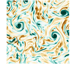
 $(\unicode[STIX]{x1D714}_{\Vert })$, on a normal (movie 5) and a parallel plane (movie 6). Altogether, the visualizations indicate that rotation destroys the small structures and modulates the flow field such that columns elongated in the direction of rotation emerge. These typical features of rotating turbulence are better appreciated in movies 3 and 4, where the pairing and stretching of co-rotating eddies are more salient.
To give an impression of the flow field, we include two snapshots in figure 2(b,c) for the run with  $Ro_{\unicode[STIX]{x1D700}}=0.06$ (strongest rotation) at times subsequent to the onset of rotation (
 $t=10.5\unicode[STIX]{x1D70F}_{f}$ and
 $t=20\unicode[STIX]{x1D70F}_{f}$) and visualizations of
 $\unicode[STIX]{x1D714}_{\Vert }$ for different
 $Ro_{\unicode[STIX]{x1D700}}$ in figures 3 and 4.
Instantaneous contours on an  $x_{1}x_{2}$ plane of the vorticity projected along the axis of rotation: (a) isotropic case; (b)
 $Ro_{\unicode[STIX]{x1D700}}=0.22$; (c)
 $Ro_{\unicode[STIX]{x1D700}}=0.06$. All panels correspond to the final simulation time
 $t\approx 30\unicode[STIX]{x1D70F}_{f}$.

Instantaneous contours on an  $x_{2}x_{3}$ plane of the vorticity projected on the axis of rotation: (a) isotropic case; (b)
 $Ro_{\unicode[STIX]{x1D700}}=0.22$; (c)
 $Ro_{\unicode[STIX]{x1D700}}=0.06$. All panels correspond to the final simulation time
 $t\approx 30\unicode[STIX]{x1D70F}_{f}$.

3 The growth rate of columnar eddies
Now, we present results and discuss the influence of different rotation rates on the growth of the columnar eddies. For the quantitative analysis, we use integral length scales, which on the one hand can be used to quantify the typical eddy size that contributes the most to the total kinetic energy, and on the other hand also serve as an indicator of anisotropy. Owing to the background rotation, the dynamics of the flow in the parallel and transverse directions are essentially different, which is reflected in the temporal evolution of  $\ell _{\Vert }$ and
 $\ell _{\bot }$ (Bardina, Ferziger & Rogallo Reference Bardina, Ferziger and Rogallo1985). As will be seen, the appearance of the columnar eddies in figures 2(b) and 2(c) is strongly reflected in the growth of the integral length scale along the axis of rotation.
We obtain the time evolution of  $\ell _{\Vert }$ and
 $\ell _{\bot }$ by evaluating (2.6) on a series of instantaneous velocity fields throughout the simulation time; see figure 5. We choose to split the actual data into two diagrams, which are displayed side by side. The left panels correspond to cases for which
 $Ro_{\unicode[STIX]{x1D700}}\geqslant 0.39$ (group R1 in table 2) and the right panels to
 $Ro_{\unicode[STIX]{x1D700}}\leqslant 0.31$ (group R2 in table 2).
Time evolution of the transverse and parallel integral length scales  $\ell _{\bot }$ and
 $\ell _{\Vert }$, for (a,c) group R1 (
 $1.54\geqslant Ro_{\unicode[STIX]{x1D700}}\geqslant 0.39$) and (b,d) group R2 (
 $0.31\geqslant Ro_{\unicode[STIX]{x1D700}}\geqslant 0.06$).

For  $Ro_{\unicode[STIX]{x1D700}}\geqslant 0.39$ (group R1, figure 5a,c),
 $\ell _{\Vert }$ and
 $\ell _{\bot }$ remain approximately unchanged in time and at values similar to the ones at
 $t=0$, which corresponds to the initial isotropic field. Specifically for
 $Ro_{\unicode[STIX]{x1D700}}=0.39$, the run with highest rotation rate in this group, the departure from isotropy is marginal and
 $\ell _{\Vert }/\ell _{\bot }\approx 1.5$ at the final simulation time. Differently, for
 $Ro_{\unicode[STIX]{x1D700}}\leqslant 0.31$ (group R2, figure 5b,d), the disparity between
 $\ell _{\Vert }$ and
 $\ell _{\bot }$ is clear. We observe that
 $\ell _{\Vert }$ grows substantially in time, whereas variations in
 $\ell _{\bot }$ are small when compared to the latter. For instance, for
 $Ro_{\unicode[STIX]{x1D700}}=0.06$, the final value of
 $\ell _{\Vert }$ is 35.05 times greater that its initial value, whereas
 $\ell _{\bot }$ only increases by a factor of 1.21. Additionally, we observe an intriguing behaviour in
 $\ell _{\bot }$. It initially grows in time until a maximum is reached; thereupon, it decreases towards a minimum, before growing again. On the other hand,
 $\ell _{\Vert }$ increases monotonically and approximately linearly for
 $t>10\unicode[STIX]{x1D70F}_{f}$.
The growth of  $\ell _{\Vert }$ in figure 5(d) is in agreement with the formation of columnar eddies observed in figure 2(c). In order to identify the dependence between the growth rate of
 $\ell _{\Vert }$ and
 $Ro_{\unicode[STIX]{x1D700}}$, we have fitted the data for
 $\ell _{\Vert }$ in the interval
 $10\unicode[STIX]{x1D70F}_{f}<t<30\unicode[STIX]{x1D70F}_{f}$ with a straight line. The linear fit approximates fairly well the time evolution of
 $\ell _{\Vert }$ and the maximum residuum is found for
 $Ro_{\unicode[STIX]{x1D700}}=0.11$, where the discrepancy is around 4.7 % of the mean value of
 $\ell _{\Vert }$. The slope of the linear fit non-dimensionalized with the forcing parameters, i.e.
 $\unicode[STIX]{x1D6FE}=\unicode[STIX]{x1D705}_{f}\unicode[STIX]{x1D70F}_{f}(\text{d}\ell _{\Vert }/\text{d}t)$, is shown in figure 6 as a function of
 $Ro_{\unicode[STIX]{x1D700}}$. For
 $Ro_{\unicode[STIX]{x1D700}}\geqslant 0.39$, the effects of rotation are irrelevant and
 $\unicode[STIX]{x1D6FE}$ is approximately zero within statistical error, suggesting that the integral length scales remain approximately at their initial value. More precisely, the linear regression leads to both positive and negative values of
 $\unicode[STIX]{x1D6FE}$ in this range. Nevertheless, the values are all very small and at most of the order of
 $O(10^{-3})$. On the other hand, the range
 $0.06\leqslant Ro_{\unicode[STIX]{x1D700}}\leqslant 0.31$ is marked by a significant rise in
 $\unicode[STIX]{x1D6FE}$, and, specifically for this range, a least-squares fit yields the power law
 $\unicode[STIX]{x1D6FE}=a\exp (b\,Ro_{\unicode[STIX]{x1D700}})$ with
 $a=3.90$ and
 $b=-16.72$ (figure 6b).
Non-dimensional growth rate  $\unicode[STIX]{x1D6FE}=\unicode[STIX]{x1D705}_{f}\unicode[STIX]{x1D70F}_{f}(\text{d}\ell _{\Vert }/\text{d}t)$ as a function of
 $Ro_{\unicode[STIX]{x1D700}}$. The least-squares fit (——) for the range
 $0.06\leqslant Ro_{\unicode[STIX]{x1D700}}\leqslant 0.31$ yields the power law
 $\unicode[STIX]{x1D6FE}=a\exp (b\,Ro_{\unicode[STIX]{x1D700}})$ with
 $a=3.90$ and
 $b=-16.72$. The thin dashed line (– – –) represents a law of the type
 $\unicode[STIX]{x1D6FE}\sim Ro_{\unicode[STIX]{x1D700}}^{-1}$, where the constant of proportionality was arbitrarily chosen to fit the leftmost data point. The dot-dashed line (– ⋅ – ⋅ –) represents a zero growth rate.

A linear growth rate for  $\ell _{\Vert }$ is in agreement with experimental observations (Jacquin et al. Reference Jacquin, Leuchter, Cambon and Mathieu1990; Staplehurst et al. Reference Staplehurst, Davidson and Dalziel2008), numerical simulations (Bartello et al. Reference Bartello, Métais and Lesieur1994; Yoshimatsu, Midorikawa & Kaneda Reference Yoshimatsu, Midorikawa and Kaneda2011) and closure theories such as the EDQNM2 of Cambon & Jacquin (Reference Cambon and Jacquin1989). Nevertheless, the growth rate obtained here is essentially different from what has been found in previous studies, which have mostly focused on decaying homogeneous isotropic turbulence. For example, the laboratory experiments of Staplehurst et al. (Reference Staplehurst, Davidson and Dalziel2008) and the DNS of Yoshimatsu et al. (Reference Yoshimatsu, Midorikawa and Kaneda2011) found a growth rate proportional to
 $1/\unicode[STIX]{x1D70F}_{\unicode[STIX]{x1D6FA}}=2\unicode[STIX]{x1D6FA}$, which would result in
 $\unicode[STIX]{x1D6FE}\sim Ro_{\unicode[STIX]{x1D700}}^{-1}$. As we see from figure 6, our results do not agree with such a scaling, which suggests a faster increase in
 $\unicode[STIX]{x1D6FE}$ for decreasing
 $Ro_{\unicode[STIX]{x1D700}}$. Nevertheless, it is important to remark that previous works have analysed the first initial time instants upon the onset of rotation, while our results include an extended observation time, and it is therefore a prediction of the growth rate of columnar eddies at later time instants. For example, the numerical results by Yoshimatsu et al. (Reference Yoshimatsu, Midorikawa and Kaneda2011) consider a total simulation time of
 $10\unicode[STIX]{x1D70F}_{\unicode[STIX]{x1D6FA}}$ for their strongest rotation case (
 $Ro_{\unicode[STIX]{x1D706}}=0.90$), whereas our results for a similar parameter point (run18,
 $Ro_{\unicode[STIX]{x1D706}}=0.80$) contain approximately
 $270\unicode[STIX]{x1D70F}_{\unicode[STIX]{x1D6FA}}$. Last, let us remark that the transition Rossby number found here (based on the disparity between
 $\ell _{\Vert }$ and
 $\ell _{\bot }$) is in close agreement with previous observations: for instance, Moisy et al. (Reference Moisy, Morize, Rabaud and Sommeria2011) report that anisotropy develops in decaying rotating turbulence at a macro and a micro Rossby number of 0.4 and 1.8, respectively. In comparison, results in figure 6 suggest a transition within the range
 $0.31<Ro_{\unicode[STIX]{x1D700}}<0.39$, which corresponds to
 $2.32<Ro_{\unicode[STIX]{x1D706}}<2.91$.
Note that to prevent the results from being affected by numerical artifacts, we stopped the simulations when  $\ell _{\Vert }$ was approximately eight times smaller than
 $2\unicode[STIX]{x03C0}{\mathcal{L}}_{\Vert }$. This constraint limited our runs to a duration of
 $30\unicode[STIX]{x1D70F}_{f}$ (
 $12.7T_{e}$), and was due to the simulation with
 $Ro_{\unicode[STIX]{x1D700}}=0.06$. Obviously, for the remaining cases,
 $2\unicode[STIX]{x03C0}{\mathcal{L}}_{\Vert }/\ell _{\Vert }>8$ at
 $t=30\unicode[STIX]{x1D70F}_{f}$. The decision of when to interrupt the runs was rather arbitrary, but a value of eight for the ratio
 $2\unicode[STIX]{x03C0}{\mathcal{L}}_{\Vert }/\ell _{\Vert }$ is common in DNS of homogeneous isotropic turbulence (Cardesa, Vela-Martín & Jiménez Reference Cardesa, Vela-Martín and Jiménez2017).
4 Scaling laws for the energy dissipation rate
The analysis for the integral length scales in the previous section has identified two regimes in our dataset. Whereas the group of runs R1 display a dynamics similar to homogeneous isotropic turbulence with no characteristic growth of  $\ell _{\Vert }$, runs in the group R2 are characterized by strong anisotropy and
 $\unicode[STIX]{x1D6FE}>0$. In this section, we present results for the evolution of the energy dissipation rate and seek similarity relations that can collapse the data in the different regimes.
Time evolution of (a) box-averaged kinetic energy  $K$ and (b) energy dissipation rate
 $\unicode[STIX]{x1D700}_{\unicode[STIX]{x1D708}}$. (c) The ratio between the normal (
 $\unicode[STIX]{x1D700}_{\unicode[STIX]{x1D708},\bot }$) and parallel (
 $\unicode[STIX]{x1D700}_{\unicode[STIX]{x1D708},\Vert }$) energy dissipation rates; (d) the data from panel (c) averaged over the interval
 $15\unicode[STIX]{x1D70F}_{f}<t<30\unicode[STIX]{x1D70F}_{f}$ and in terms of
 $Ro_{\unicode[STIX]{x1D700}}$.

After the onset of rotation, both  $K$ and
 $\unicode[STIX]{x1D700}_{\unicode[STIX]{x1D708}}$ evolve in time according to the conservation of energy, i.e.
 $\text{d}K/\text{d}t=-\unicode[STIX]{x1D700}_{\unicode[STIX]{x1D708}}+\unicode[STIX]{x1D700}_{I}$. While
 $K$ grows rapidly (figure 7a), the viscous dissipation
 $\unicode[STIX]{x1D700}_{\unicode[STIX]{x1D708}}$ first decreases monotonically until a minimum (figure 7b). The minimum value decreases with
 $Ro_{\unicode[STIX]{x1D700}}$, and for the runs of group R2 it scales with
 $Ro_{\unicode[STIX]{x1D700}}^{0.36}$ (not shown). After reaching its lowest value,
 $\unicode[STIX]{x1D700}_{\unicode[STIX]{x1D708}}$ continues to grow towards the power input
 $\unicode[STIX]{x1D700}_{I}$, although the inequality
 $\unicode[STIX]{x1D700}_{\unicode[STIX]{x1D708}}<\unicode[STIX]{x1D700}_{I}$ remains for some of the cases up to the final simulation time. Generally speaking, the mismatch between the energy dissipation rate and the energy input rate in figure 7(b) is stronger for small
 $Ro_{\unicode[STIX]{x1D700}}$ (group R2). For the runs in this group, we also observe that the parallel direction contributes significantly to
 $\unicode[STIX]{x1D700}_{\unicode[STIX]{x1D708}}$ (figure 7c). By splitting the energy dissipation rate into its normal and parallel contributions such that
 $\unicode[STIX]{x1D700}_{\unicode[STIX]{x1D708}}=2\unicode[STIX]{x1D700}_{\unicode[STIX]{x1D708},\bot }+\unicode[STIX]{x1D700}_{\unicode[STIX]{x1D708},\Vert }$, where
 $\unicode[STIX]{x1D700}_{\unicode[STIX]{x1D708},\bot }=(\unicode[STIX]{x1D700}_{\unicode[STIX]{x1D708},11}+\unicode[STIX]{x1D700}_{\unicode[STIX]{x1D708},22})/2$ and
 $\unicode[STIX]{x1D700}_{\unicode[STIX]{x1D708},\Vert }=\unicode[STIX]{x1D700}_{\unicode[STIX]{x1D708},33}$, we find that, for decreasing
 $Ro_{\unicode[STIX]{x1D700}}$, the contribution due to the parallel direction increases, whereas for large
 $Ro_{\unicode[STIX]{x1D700}}$ the energy dissipation rate is equally partitioned among both directions. For instance, for
 $Ro_{\unicode[STIX]{x1D700}}=1.54$ the ratio
 $\unicode[STIX]{x1D700}_{\unicode[STIX]{x1D708},\bot }/\unicode[STIX]{x1D700}_{\unicode[STIX]{x1D708},\Vert }$ is close to 1, while for
 $Ro_{\unicode[STIX]{x1D700}}=0.06$ almost half of the total dissipation stems from
 $\unicode[STIX]{x1D700}_{\unicode[STIX]{x1D708},\Vert }$. In figure 7(c), we also note that
 $\unicode[STIX]{x1D700}_{\unicode[STIX]{x1D708},\bot }/\unicode[STIX]{x1D700}_{\unicode[STIX]{x1D708},\Vert }$ remains approximately unchanged in time for
 $t>15\unicode[STIX]{x1D70F}_{f}$. Averaging
 $\unicode[STIX]{x1D700}_{\unicode[STIX]{x1D708},\bot }/\unicode[STIX]{x1D700}_{\unicode[STIX]{x1D708},\Vert }$ (figure 7d) in the interval
 $15\unicode[STIX]{x1D70F}_{f}<t<30\unicode[STIX]{x1D70F}_{f}$ shows that
 $\unicode[STIX]{x1D700}_{\unicode[STIX]{x1D708},\bot }/\unicode[STIX]{x1D700}_{\unicode[STIX]{x1D708},\Vert }$ scales with
 $Ro_{\unicode[STIX]{x1D700}}^{0.37}$ for
 $0.31<Ro_{\unicode[STIX]{x1D700}}<0.14$, while for smaller
 $Ro_{\unicode[STIX]{x1D700}}$ the ratio between normal and parallel dissipation rates seems to reach an asymptotic limit of 0.54 for
 $Ro_{\unicode[STIX]{x1D700}}<0.9$. The latter finding, however, needs to be confirmed by studies at even lower
 $Ro_{\unicode[STIX]{x1D700}}$.
The imbalance  $\unicode[STIX]{x1D700}_{\unicode[STIX]{x1D708}}\neq \unicode[STIX]{x1D700}_{I}$ is the footprint of an inverse energy cascade that is triggered by the Coriolis force, and that leads to the accumulation of energy at the large scales. This is expected to occur when
 $Ro_{\unicode[STIX]{x1D700}}$ is below a critical Rossby number that depends on the geometrical dimensions of the system (Smith, Chasnov & Waleffe Reference Smith, Chasnov and Waleffe1996; Deusebio et al. Reference Deusebio, Boffetta, Lindborg and Musacchio2014; Pestana & Hickel Reference Pestana and Hickel2019b). In such cases, however, equilibrium
 $(\unicode[STIX]{x1D700}_{\unicode[STIX]{x1D708}}=\unicode[STIX]{x1D700}_{I})$ can still be restored after long integration times when the energy in the wavenumbers
 $\unicode[STIX]{x1D705}<\unicode[STIX]{x1D705}_{f}$ is sufficiently high to contribute to
 $\unicode[STIX]{x1D700}_{\unicode[STIX]{x1D708}}$ (Valente & Dallas Reference Valente and Dallas2017; Seshasayanan & Alexakis Reference Seshasayanan and Alexakis2018). For the runs considered in this study, the critical
 $Ro_{\unicode[STIX]{x1D700}}$ is approximately 1, as shown in Pestana & Hickel (Reference Pestana and Hickel2019b).
From figure 7(b), it is evident that a naive scaling in terms of the forcing parameters cannot cause the different lines in figure 7(b) to collapse, as it would in homogeneous isotropic turbulence. In other words, an approximation of  $\unicode[STIX]{x1D700}_{\unicode[STIX]{x1D708}}$ in terms of
 $u_{f}$ and
 $\unicode[STIX]{x1D705}_{f}$ is invalid because the evolution of
 $\unicode[STIX]{x1D700}_{\unicode[STIX]{x1D708}}$ in figure 7(b) depends clearly on
 $Ro_{\unicode[STIX]{x1D700}}$. In homogeneous isotropic turbulence, the estimation
 $\unicode[STIX]{x1D700}_{\unicode[STIX]{x1D708}}\sim u_{f}^{3}\unicode[STIX]{x1D705}_{f}$ suffices since both
 $u_{f}$ and
 $1/\unicode[STIX]{x1D705}_{f}$ are proportional to a characteristic velocity and a characteristic length, and this expression is equivalent to
 $\unicode[STIX]{x1D700}_{\unicode[STIX]{x1D708}}\sim ({u^{\prime }}^{iso})^{3}/\ell ^{iso}$. We must therefore search for other ways to approximate
 $\unicode[STIX]{x1D700}_{\unicode[STIX]{x1D708}}$ in rotating turbulence.
4.1 Spectral transfer time
To address this problem, we followed the methodology introduced by Kraichnan (Reference Kraichnan1965) within the context of MHD and bridged by Zhou (Reference Zhou1995) to homogeneous rotating flows. The basic idea is that the rate at which energy is transferred to the smaller scales depends on an energy content and on a time scale, viz. the spectral transfer time. If we treat the characteristic scales as global quantities instead of being wavenumber-dependent, the dissipation law can be written in terms of the r.m.s. velocity and the spectral transfer time as
 $$\begin{eqnarray}\unicode[STIX]{x1D700}_{\unicode[STIX]{x1D708}}\sim \frac{{u^{\prime }}^{2}}{\unicode[STIX]{x1D70F}_{s}}.\end{eqnarray}$$
The spectral transfer time, however, is composed of two additional time scales, namely the nonlinear time scale  $\unicode[STIX]{x1D70F}_{nl}$ and the relaxation time scale
 $\unicode[STIX]{x1D70F}_{3}$. Whereas
 $\unicode[STIX]{x1D70F}_{nl}$ indicates how fast the triple velocity correlations are built up and favours the forward energy cascade,
 $\unicode[STIX]{x1D70F}_{3}$ serves as a relaxation time or a measure of how fast the triple velocity correlations are destroyed. The assumptions that the energy dissipation rate
 $\unicode[STIX]{x1D700}_{\unicode[STIX]{x1D708}}$ is directly proportional to
 $\unicode[STIX]{x1D70F}_{3}$ and that the energy cascade is local lead to the so-called ‘golden rule’ (Zhou Reference Zhou1995):
 $$\begin{eqnarray}\unicode[STIX]{x1D70F}_{s}\sim \frac{\unicode[STIX]{x1D70F}_{nl}^{2}}{\unicode[STIX]{x1D70F}_{3}}.\end{eqnarray}$$
In (4.2),  $\unicode[STIX]{x1D70F}_{nl}$ involves a velocity and a length scale and
 $\unicode[STIX]{x1D70F}_{3}$ can rest on any other time scales that are relevant for the problem. For instance, in forced homogeneous isotropic flows,
 $\unicode[STIX]{x1D70F}_{3}\sim \unicode[STIX]{x1D70F}_{f}\sim \unicode[STIX]{x1D70F}_{nl}\sim \ell ^{iso}/{u^{\prime }}^{iso}$, which implies
 $\unicode[STIX]{x1D70F}_{s}\sim \ell ^{iso}/{u^{\prime }}^{iso}$ to recover the well-known dissipation law
 $\unicode[STIX]{x1D700}_{\unicode[STIX]{x1D708}}\sim ({u^{\prime }}^{iso})^{3}/\ell ^{iso}$, extensively verified by DNS and experiments. For more complex flows, which involve other time scales like rotating turbulence with the rotation time scale
 $\unicode[STIX]{x1D70F}_{\unicode[STIX]{x1D6FA}}=1/(2\unicode[STIX]{x1D6FA})$, the relaxation time scale
 $\unicode[STIX]{x1D70F}_{3}$ can be assumed as a function of the type
 $\unicode[STIX]{x1D70F}_{3}=\unicode[STIX]{x1D70F}_{3}(\unicode[STIX]{x1D70F}_{f},\unicode[STIX]{x1D70F}_{\unicode[STIX]{x1D6FA}})$ (Kraichnan Reference Kraichnan1965; Matthaeus & Zhou Reference Matthaeus and Zhou1989; Zhou Reference Zhou1995). Combining (4.1) and (4.2) leads to
 $$\begin{eqnarray}\unicode[STIX]{x1D700}_{\unicode[STIX]{x1D708}}\sim {u^{\prime }}^{2}\left(\frac{\unicode[STIX]{x1D70F}_{3}}{\unicode[STIX]{x1D70F}_{nl}^{2}}\right),\end{eqnarray}$$
and the problem of determining the dissipation law becomes the one of determining  $\unicode[STIX]{x1D70F}_{nl}$ and
 $\unicode[STIX]{x1D70F}_{3}$.
4.2 Evaluation of current available dissipation laws
In the current literature, a few dissipation laws for homogeneous rotating turbulence have been proposed. For example, the approximations that follow from the theory of Zhou (Reference Zhou1995), Galtier (Reference Galtier2003), Nazarenko & Schekochihin (Reference Nazarenko and Schekochihin2011) and Baqui & Davidson (Reference Baqui and Davidson2015) are
 $$\begin{eqnarray}\unicode[STIX]{x1D700}_{\unicode[STIX]{x1D708}}\sim \frac{{u^{\prime }}^{4}}{\unicode[STIX]{x1D6FA}\ell ^{2}},\quad \unicode[STIX]{x1D700}_{\unicode[STIX]{x1D708}}\sim \frac{{u^{\prime }}^{4}\ell _{\Vert }}{\unicode[STIX]{x1D6FA}\ell _{\bot }^{3}},\quad \unicode[STIX]{x1D700}_{\unicode[STIX]{x1D708}}\sim \frac{{u^{\prime }}^{3}}{\ell _{\bot }}\quad \text{and}\quad \unicode[STIX]{x1D700}_{\unicode[STIX]{x1D708}}\sim \frac{{u^{\prime }}^{3}}{\ell _{\Vert }},\end{eqnarray}$$
respectively. Although these authors do not explicitly present their theories within the framework of a spectral transfer time, we have taken the freedom to also summarize the theories within this context.
The law proposed by Zhou (Reference Zhou1995), for instance, ignores anisotropy. It assumes that  $\unicode[STIX]{x1D70F}_{nl}\sim \ell /u^{\prime }$ and that the relaxation time scale is proportional to the rotation time scale, i.e.
 $\unicode[STIX]{x1D70F}_{3}\sim \unicode[STIX]{x1D70F}_{\unicode[STIX]{x1D6FA}}$, to yield
 $\unicode[STIX]{x1D700}_{\unicode[STIX]{x1D708}}\sim {u^{\prime }}^{4}/(\unicode[STIX]{x1D6FA}\ell ^{2})$. In contrast, dimensional analysis for the weak inertial-wave theory proposed by Galtier (Reference Galtier2003), which takes into account scale anisotropy, results in
 $\unicode[STIX]{x1D700}_{\unicode[STIX]{x1D708}}\sim {u^{\prime }}^{4}\ell _{\Vert }/(\unicode[STIX]{x1D6FA}\ell _{\bot }^{3})$, where
 $\unicode[STIX]{x1D70F}_{nl}\sim \ell _{\bot }/u^{\prime }$ and
 $\unicode[STIX]{x1D70F}_{3}\sim \ell _{\Vert }/(\unicode[STIX]{x1D6FA}\ell _{\bot })$. When anisotropy is disregarded, however, i.e.
 $\ell \sim \ell _{\Vert }\sim \ell _{\bot }$, the predictions by Galtier (Reference Galtier2003) reduce to the relation proposed by Zhou (Reference Zhou1995). The critical balance theory of Nazarenko & Schekochihin (Reference Nazarenko and Schekochihin2011) considers that
 $\unicode[STIX]{x1D70F}_{nl}\sim \unicode[STIX]{x1D70F}_{3}\sim \ell _{\bot }/u^{\prime }$ and the theory of Baqui & Davidson (Reference Baqui and Davidson2015) suggests that
 $\unicode[STIX]{x1D70F}_{nl}\sim \unicode[STIX]{x1D70F}_{3}\sim \ell _{\Vert }/u^{\prime }$.
When we apply the scaling laws in (4.4) to the data presented in figure 7(b), we find a good match for the runs in group R1. In figures 8 and 9, we scale  $\unicode[STIX]{x1D700}_{\unicode[STIX]{x1D708}}$ with the different laws; figure 9 shows the inverse of what appears in figure 8. We present the results in this manner in order to provide a fair treatment and avoid misinterpretations from arbitrary choice of the axis limits, which can increase/decrease the spread between the lines.
Compensated time evolution of the energy dissipation rate for  $0.06\leqslant Ro_{\unicode[STIX]{x1D700}}\leqslant 1.54$. The various panels correspond to the different scaling laws found in the literature: (a) Zhou (Reference Zhou1995); (b) weak inertial-wave theory of Galtier (Reference Galtier2003); (c) critical balance theory of Nazarenko & Schekochihin (Reference Nazarenko and Schekochihin2011); and (d) Baqui & Davidson (Reference Baqui and Davidson2015).

Compensated time evolution of the energy dissipation rate as in figure 8, but plotted as the inverse. The various panels correspond to the different scaling laws found in the literature: (a) Zhou (Reference Zhou1995); (b) weak inertial-wave theory of Galtier (Reference Galtier2003); (c) critical balance theory of Nazarenko & Schekochihin (Reference Nazarenko and Schekochihin2011); and (d) Baqui & Davidson (Reference Baqui and Davidson2015).

By comparing figures 8(a) and 9(a), we see that the approximation suggested by Zhou (Reference Zhou1995) cannot collapse the data. Whereas the data for the group R2 appears close to straight lines in figure 9(a), figure 8(a) shows that they diverge and instead increase in time. For large  $Ro_{\unicode[STIX]{x1D700}}$, however, both figures show straight lines, suggesting a correction factor in terms of
 $Ro_{\unicode[STIX]{x1D700}}$. For the weak inertial-wave theory, figure 8(b) shows that the curves of the last five runs in group R2 (lowest
 $Ro_{\unicode[STIX]{x1D700}}$) seem to follow a similar trend. This behaviour, however, is not observed in figure 9(b), which shows that these lines actually increase in time with approximately the same slope. For the runs in group R1, figure 9(b) shows a reasonable collapse of the data, which is, however, opposed by figure 8(b). The predictions by Nazarenko & Schekochihin (Reference Nazarenko and Schekochihin2011) in figures 8(c) and 9(c) show that, for large
 $Ro_{\unicode[STIX]{x1D700}}$, the curves are flat and tend closer to each other. This is expected, as
 $\ell _{\bot }$ must tend to
 $\ell ^{iso}$ for large
 $Ro_{\unicode[STIX]{x1D700}}$, and in this limit the dissipation law of homogeneous isotropic turbulence is recovered. For small
 $Ro_{\unicode[STIX]{x1D700}}$, this scaling delivers approximately straight lines in both diagrams, which suggests that a correction in terms of
 $Ro_{\unicode[STIX]{x1D700}}$ might also be possible.
The best approximation, at least for part of the dataset (group R1), is obtained with the scaling law of Baqui & Davidson (Reference Baqui and Davidson2015). Figures 8(d) and 9(d) indicate that this scaling is suitable for the runs in group R1 (indicated with an arrow in the figures). For the other runs (group R2), figures 8(d) and 9(d) also provide unsatisfactory results. We are then motivated to look into a similarity law for this group of runs.
4.3 A dissipation scaling law for runs in group R2
To find a dissipation law for runs in group R2, we base ourselves on (4.3). The first question we turn to is the one of finding an approximation for  $\unicode[STIX]{x1D70F}_{nl}$. The nonlinear time scale involves an estimation of a velocity and a length scale, which we shall assume as
 $u^{\prime }$ and
 $\ell _{\bot }$, respectively. The reason behind this choice goes as follows. From figures 5(d) and 7(b), we observe that
 $\ell _{\bot }$ and
 $\unicode[STIX]{x1D700}_{\unicode[STIX]{x1D708}}$ display similar dynamics, although inverse; the evolution of each variable is the opposite of the other. This behaviour hints at a dependence of the form
 $\unicode[STIX]{x1D700}_{\unicode[STIX]{x1D708}}\sim 1/\ell _{\bot }$, which can also be justified like in the critical balance theory (Nazarenko & Schekochihin Reference Nazarenko and Schekochihin2011). Within this theory, the basic idea is that rotation tends to destroy derivatives along the direction of rotation, and the advection term is mainly due to the normal velocity gradients and the normal velocity field. Thus,
 $\ell _{\bot }$ is taken as the relevant length scale for the nonlinear interactions. On the other hand, for the velocity scale, an alternative would be to take information about the transverse velocity fields only as in Baqui & Davidson (Reference Baqui and Davidson2015). Nevertheless, although rotation favours two-dimensionalization, the velocity field remains three-component and the anisotropy in the Reynolds stress tensor is minimal (Yeung & Zhou Reference Yeung and Zhou1998). For the above reasons, we assume
 $\unicode[STIX]{x1D70F}_{nl}\sim \ell _{\bot }/u^{\prime }$, and in a preliminary step (4.3) can be expressed as
 $$\begin{eqnarray}\unicode[STIX]{x1D700}_{\unicode[STIX]{x1D708}}\sim \frac{{u^{\prime }}^{4}}{\ell _{\bot }^{2}}\unicode[STIX]{x1D70F}_{3}(\unicode[STIX]{x1D70F}_{f},\unicode[STIX]{x1D70F}_{\unicode[STIX]{x1D6FA}}).\end{eqnarray}$$
Decorrelation (relaxation) time scale  $\unicode[STIX]{x1D70F}_{3}$: (a) as a function of time and (b) averaged over the interval
 $10\leqslant t\leqslant 30\unicode[STIX]{x1D70F}_{f}$ and normalized by the nonlinear time scale
 $\unicode[STIX]{x1D70F}_{nl}^{iso}$ times the proportionality constant
 $C_{\unicode[STIX]{x1D700}}^{iso}$. Two reference lines are included in panel (b). The horizontal line at the top signals that, for large
 $Ro_{\unicode[STIX]{x1D700}}$, the relaxation time scale tends to the value of the nonlinear time scale of the homogeneous isotropic case. The other line shows the power-law dependence of the type
 $Ro_{\unicode[STIX]{x1D700}}^{h}$ with
 $h=0.62$ for runs of the group R2.

Now, to determine the relaxation time scale, we rearrange (4.5) so that  $\unicode[STIX]{x1D70F}_{3}$ appears as a function of the other terms and we examine its temporal evolution. Figure 10(a) shows
 $\unicode[STIX]{x1D70F}_{3}\sim \unicode[STIX]{x1D700}_{\unicode[STIX]{x1D708}}\,\ell _{\bot }^{2}/{u^{\prime }}^{4}$ over time for all runs. After a transient of approximately
 $10\unicode[STIX]{x1D70F}_{f}$, we observe that the curves for different
 $Ro_{\unicode[STIX]{x1D700}}$ reach a plateau, with a terminal value that depends on
 $Ro_{\unicode[STIX]{x1D700}}$. To determine this dependence, results from figure 10(a) are then averaged in the interval
 $10\unicode[STIX]{x1D70F}_{f}<t<30\unicode[STIX]{x1D70F}_{f}$ and the mean value is shown against the corresponding Rossby number in figure 10(b). In the latter, the ordinates appear normalized by the nonlinear time scale
 $\unicode[STIX]{x1D70F}_{nl}^{iso}$ times
 $C_{\unicode[STIX]{x1D700}}^{iso}$, which is the constant of proportionality of the dissipation law in homogeneous isotropic turbulence. For runs in group R1,
 $\unicode[STIX]{x1D70F}_{3}/(\unicode[STIX]{x1D70F}_{nl}^{iso}C_{\unicode[STIX]{x1D700}}^{iso})$ increases with
 $Ro_{\unicode[STIX]{x1D700}}$ and asymptotically approaches 1, implying that for these
 $Ro_{\unicode[STIX]{x1D700}}$ the effects of rotation are negligible and the scaling law of homogeneous isotropic turbulence is recovered. Contrarily, and more surprising, we see that
 $\unicode[STIX]{x1D70F}_{3}/(\unicode[STIX]{x1D70F}_{nl}^{iso}C_{\unicode[STIX]{x1D700}}^{iso})$ follows the power law
 $Ro_{\unicode[STIX]{x1D700}}^{h}$ with
 $h=0.62$ for the runs in group R2. Consequently, for this group, we can finally express (4.5) as
 $$\begin{eqnarray}\unicode[STIX]{x1D700}_{\unicode[STIX]{x1D708}}\sim \frac{{u^{\prime }}^{4}}{\ell _{\bot }^{2}}(\unicode[STIX]{x1D70F}_{nl}^{iso}Ro_{\unicode[STIX]{x1D700}}^{0.62})\sim \frac{{u^{\prime }}^{3}}{\ell _{\bot }}\left[\left(\frac{\unicode[STIX]{x1D70F}_{nl}^{iso}}{\unicode[STIX]{x1D70F}_{nl}}\right)Ro_{\unicode[STIX]{x1D700}}^{0.62}\right].\end{eqnarray}$$
Equation (4.6) summarizes the effects of rotation for the runs with  $0.06\leqslant Ro_{\unicode[STIX]{x1D700}}\leqslant 0.31$, and suggests that, in a rotating frame of reference, the disparity between
 $\unicode[STIX]{x1D70F}_{nl}$ and
 $\unicode[STIX]{x1D70F}_{nl}^{iso}$ increases, such that the ratio
 $(\unicode[STIX]{x1D70F}_{nl}/\unicode[STIX]{x1D70F}_{nl}^{iso})$ shrinks with the inverse of
 $Ro_{\unicode[STIX]{x1D700}}^{0.62}$. In other words, equation (4.6) implies that the relaxation time scale is
 $\unicode[STIX]{x1D70F}_{3}\sim \unicode[STIX]{x1D70F}_{nl}^{iso}Ro_{\unicode[STIX]{x1D700}}^{0.62}$. Finally, scaling the data in figure 7(b) with (4.6) leads to figure 11, where very good agreement is found for all the cases in group R2.
Time evolution of the energy dissipation rate scaled according to (4.6) for  $0.06\leqslant Ro_{\unicode[STIX]{x1D700}}\leqslant 0.31$.

4.4 Energy spectra
With a dissipation law at hand, phenomenological arguments can be further employed to obtain predictions for the scaling exponents of the different energy spectra. In fact, the different theories presented in (4.4) are associated with predictions for the kinetic energy spectra. Strictly speaking, the validation of scaling laws for the energy spectra requires data with a well-defined inertial range, in which the spectral energy flux is constant and equals  $\unicode[STIX]{x1D700}_{\unicode[STIX]{x1D708}}$ for a wide range of wavenumbers. In our runs, the latter does not apply due to the relatively low
 $Re_{\unicode[STIX]{x1D706}}$ (see figure 12).
Energy spectra at the last instant of time, i.e.  $t=30\unicode[STIX]{x1D70F}_{f}$, for every other case in table 2: (a,c,e) cases of group R1, and (b,d,f) cases of group R2. (a,b) Spherical energy spectra; (c,d) normal energy spectra; and (e,f) longitudinal energy spectra. The grey dashed line (


If we assume that the energy cascade is local, dimensional analysis leads to (Zhou Reference Zhou1995)
 $$\begin{eqnarray}\unicode[STIX]{x1D700}_{\unicode[STIX]{x1D708}}\sim \left(\frac{\unicode[STIX]{x1D70F}_{3}}{\unicode[STIX]{x1D70F}_{nl}^{2}}\right)\unicode[STIX]{x1D705}_{\Vert }\unicode[STIX]{x1D705}_{\bot }E(\unicode[STIX]{x1D705}_{\bot },\unicode[STIX]{x1D705}_{\Vert }).\end{eqnarray}$$
In the equation above, the energy content of a scale of typical size  $\ell \sim 1/\unicode[STIX]{x1D705}$ was assumed to be of the order of
 $\unicode[STIX]{x1D705}_{\Vert }\unicode[STIX]{x1D705}_{\bot }E(\unicode[STIX]{x1D705}_{\bot },\unicode[STIX]{x1D705}_{\Vert })$, where
 $E(\unicode[STIX]{x1D705}_{\bot },\unicode[STIX]{x1D705}_{\Vert })$ is the energy spectrum and
 $\unicode[STIX]{x1D705}_{\bot }$ and
 $\unicode[STIX]{x1D705}_{\Vert }$ are the wavenumbers in the normal and longitudinal directions, respectively. Using (4.6) and (4.7), we obtain
 $E(\unicode[STIX]{x1D705}_{\bot },\unicode[STIX]{x1D705}_{\Vert })\sim B\unicode[STIX]{x1D705}_{\bot }^{-2}\unicode[STIX]{x1D705}_{\Vert }^{-1}$, with
 $B=(\unicode[STIX]{x1D700}_{\unicode[STIX]{x1D708}}Ro_{\unicode[STIX]{x1D700}}^{-0.62}/\unicode[STIX]{x1D70F}_{nl}^{iso})^{1/2}$, whereas the weak inertial-wave theory of Galtier (Reference Galtier2003) predicts that
 $E(k_{\bot },k_{\Vert })\sim k_{\bot }^{-5/2}k_{\Vert }^{-1/2}$.
A least-squares fit for the case with  $Ro_{\unicode[STIX]{x1D700}}=0.31$ indicates that
 $E(\unicode[STIX]{x1D705}_{\bot })$ varies with
 $\unicode[STIX]{x1D705}_{\bot }^{-2.54}$ in the range
 $1.2<\unicode[STIX]{x1D705}_{\bot }/\unicode[STIX]{x1D705}_{f}<6$ (figure 12d), and that
 $E(\unicode[STIX]{x1D705}_{\Vert })$ varies with
 $\unicode[STIX]{x1D705}_{\Vert }^{-0.48}$ in the range
 $0.05<\unicode[STIX]{x1D705}_{\Vert }/\unicode[STIX]{x1D705}_{f}<0.8$ (figure 12f). The exponents, however, increase with
 $Ro_{\unicode[STIX]{x1D700}}$: for
 $Ro_{\unicode[STIX]{x1D700}}=0.3$ (largest
 $Ro_{\unicode[STIX]{x1D700}}$ displayed on the right-hand panels of figure 12), we find that in the same range
 $E(\unicode[STIX]{x1D705}_{\bot })$ varies with
 $\unicode[STIX]{x1D705}_{\bot }^{-2.17}$ and that
 $E(\unicode[STIX]{x1D705}_{\Vert })$ changes with
 $\unicode[STIX]{x1D705}_{\Vert }^{-0.34}$. For the runs of group R1, we do not observe any significant changes with respect to the initial isotropic energy spectrum. Differently from the runs in R2, where there is a substantial accumulation of energy for
 $\unicode[STIX]{x1D705}<\unicode[STIX]{x1D705}_{f}$ (see e.g. figure 12b), the energy spectra for runs in group R1 are marginally altered with respect to the isotropic initial conditions (see left-hand panels in figure 12). There is also no wavenumber range with a distinctive scaling, apart from the range
 $\unicode[STIX]{x1D705}<\unicode[STIX]{x1D705}_{f}$, which scales approximately with
 $\unicode[STIX]{x1D705}^{2}$, as in the initial isotropic conditions (Dallas, Fauve & Alexakis Reference Dallas, Fauve and Alexakis2015).
5 Conclusions
We have investigated the effects of system rotation with Rossby numbers in the range  $0.06\leqslant Ro_{\unicode[STIX]{x1D700}}\leqslant 1.54$ on the evolution of an initial cloud of isotropic eddies. Differently from other studies, which have focused on the initial transient immediately after the onset of rotation, we have focused instead on longer time intervals. This was only possible because our DNS were carried out in elongated domains, which were 340 times larger than the initial characteristic eddy size.
The classical pictures of rotating turbulence were reproduced, in which we observed the formation of columnar eddies along the axis of rotation and a decrease in the energy dissipation rate. However, by following the evolution of the integral length scales, we identified different dynamics that were shown to depend on  $Ro_{\unicode[STIX]{x1D700}}$. This led us to separate our dataset into two groups. While the runs in group R1 did not show any pronounced sign of growth in the integral length scales, for the runs in group R2,
 $\ell _{\Vert }$ grew substantially and approximately linearly with time. The latter group of runs can therefore be associated with a regime where the formation of columns predominates, whereas runs of group R1 are closer to homogeneous isotropic turbulence. Further, we found that the growth rate of the columnar eddies in group R2 depends exponentially on
 $Ro_{\unicode[STIX]{x1D700}}$, i.e.
 $\unicode[STIX]{x1D6FE}=a\exp (b\,Ro_{\unicode[STIX]{x1D700}})$, with
 $a=3.90$ and
 $b=-16.72$.
The energy dissipation rate in the group of runs R1 is well approximated by the scaling law proposed in Baqui & Davidson (Reference Baqui and Davidson2015). For the group R2, which consists of runs at lower  $Ro_{\unicode[STIX]{x1D700}}$, we have shown that the scaling laws currently available in the literature fail to approximate
 $\unicode[STIX]{x1D700}_{\unicode[STIX]{x1D708}}$. Still, we were able to find a similarity relation for
 $\unicode[STIX]{x1D700}_{\unicode[STIX]{x1D708}}$ in the range
 $0.06\leqslant Ro_{\unicode[STIX]{x1D700}}\leqslant 0.31$ by applying the ideas introduced by Kraichnan (Reference Kraichnan1965), in which the spectral transfer time is regarded as composed of two opposing time scales. First, by observing the inverse relation between
 $\ell _{\bot }$ and
 $\unicode[STIX]{x1D700}_{\unicode[STIX]{x1D708}}$, we assumed that
 $\ell _{\bot }$ was the relevant length scale to form
 $\unicode[STIX]{x1D70F}_{nl}$. Second, the relaxation time scale
 $\unicode[STIX]{x1D70F}_{3}$ was shown to depend on a power law of
 $Ro_{\unicode[STIX]{x1D700}}$ and on
 $\unicode[STIX]{x1D70F}_{nl}^{iso}$, which implies that it is exclusively a function of
 $Ro_{\unicode[STIX]{x1D700}}$ and of the forcing parameters
 $\unicode[STIX]{x1D705}_{f}$ and
 $u_{f}$. Thus, we arrived at a similarity law for this
 $Ro_{\unicode[STIX]{x1D700}}$ range. Scaling
 $\unicode[STIX]{x1D700}_{\unicode[STIX]{x1D708}}$ with
 $(u^{\prime 4}Ro_{\unicode[STIX]{x1D700}}^{0.62}\unicode[STIX]{x1D70F}_{nl}^{iso})/\ell _{\bot }^{2}$ collapsed the data for different
 $Ro_{\unicode[STIX]{x1D700}}$ into a single curve.
Last, we would like to remark that the results for the case where the rotation rate is highest, i.e.  $Ro_{\unicode[STIX]{x1D700}}=0.06$, were verified by increasing the numerical resolution and the domain size by a factor of two in the direction of rotation. However, whether other dynamics emerge at even lower
 $Ro_{\unicode[STIX]{x1D700}}$ and the effects of
 $Re_{\unicode[STIX]{x1D700}}$ remain to be studied. In any case, we hope our numerical investigation contributes to the improvement of turbulence models and stimulates future studies to elucidate and quantify the effects of the Coriolis force on the evolution of a cloud of isotropic eddies in unbounded domains.
Acknowledgements
The simulations have been performed at the Dutch National Supercomputer Cartesius with the support of the SURF cooperative and the Dutch Research Council (NWO) project no. 16108. The authors would like to thank the technical expertise and the assistance provided by SURFsara.
Declaration of interests
The authors report no conflict of interest.
Supplementary movies
Supplementary movies are available at: https://doi.org/10.4121/uuid:324788e3-a64f-4786-9ef9-f97d70a29064.



