





1. Introduction
Reactive transport is ubiquitous in geological systems across multiple scales. Mineral dissolution in flowing fluids generates evolving solid–fluid interfaces governed by nonlinear couplings between transport, reaction kinetics and the evolution of the pore microstructure (Ortoleva et al. Reference Ortoleva, Chadam, Merino and Sen1987; Daccord et al. Reference Daccord, Lenormand and Liétard1993; Fredd & Fogler Reference Fredd and Fogler1998a ; Golfier et al. Reference Golfier, Zarcone, Bazin, Lenormand, Lasseux and Quintard2002; Soulaine et al. Reference Soulaine, Roman, Kovscek and Tchelepi2018). Dissolution produces complex interface dynamics, including symmetry breaking, localised sharpening or progressive surface smoothing, depending on the relative importance of advection, diffusion and surface reaction (Kang et al. Reference Kang, Chen, Valocchi and Viswanathan2014; Soulaine et al. Reference Soulaine, Roman, Kovscek and Tchelepi2017; Lee et al. Reference Lee, Chen, Bresciani, Toner and Kang2025). As the interface recedes, the flow field and concentration gradients continuously adjust, which in turn influences the local dissolution rate and further alters the geometry. This feedback is particularly strong in confined systems such as microfluidic devices and porous media, where small geometric perturbations can significantly alter transport pathways (Daccord & Lenormand Reference Daccord and Lenormand1987; Fredd & Fogler Reference Fredd and Fogler1998b ; Golfier et al. Reference Golfier, Zarcone, Bazin, Lenormand, Lasseux and Quintard2002; Szymczak & Ladd Reference Szymczak and Ladd2009).
In porous systems, numerical and experimental studies have demonstrated that the structure of dissolving fronts depends strongly on the Péclet number,
 $\textit{Pe}$
(reflecting the balance between advection and diffusion), and the Damköhler number,
 ${\textit{Da}}$
(comparing reaction kinetics to transport) (Hao et al. Reference Hao, Smith and Carroll2019; Liu et al. Reference Liu, Yan, Yao and Sun2019; Guo et al. Reference Guo, Laouafa and Quintard2021; Menke et al. Reference Menke, Maes and Geiger2023; Szawello et al. Reference Szawello, Hyman, Kang and Szymczak2026). Understanding how these dimensionless parameters govern interface evolution is essential for developing large-scale physically grounded reactive transport models (Molins et al. Reference Molins, Trebotich, Steefel and Shen2012). A broad spectrum of regimes has been identified across scales, including uniform dissolution with spatially homogeneous reactive fluxes, compact and smoothly advancing fronts, conical wormhole formation driven by localised transport, single dominant wormholes capturing most of the flow and highly ramified channel networks resulting from competitive growth (Fredd & Fogler Reference Fredd and Fogler1998b
; Golfier et al. Reference Golfier, Zarcone, Bazin, Lenormand, Lasseux and Quintard2002). Increasing
 $\textit{Pe}$
enhances transport localisation and promotes upstream–downstream asymmetries, while increasing
 ${\textit{Da}}$
amplifies reaction-driven instabilities by steepening concentration gradients near the interface. Although these regimes are typically characterised at the Darcy scale, their origin lies in pore- and grain-scale processes, where subtle variations in local geometry and hydrodynamics modulate reactive fluxes (Soulaine et al. Reference Soulaine, Roman, Kovscek and Tchelepi2017; Molins et al. Reference Molins2020).
The dissolution of a single grain constitutes a fundamental model problem that isolates the elementary mechanisms responsible for interface motion, asymmetry development and surface smoothing. Previous investigations have shown that even this canonical configuration exhibits a wide range of morphologies depending on transport-reaction conditions (Dutka et al. Reference Dutka, Starchenko, Osselin, Magni, Szymczak and Ladd2020; Ladd et al. Reference Ladd, Yu and Szymczak2020; Molins et al. Reference Molins2020; Guo et al. Reference Guo, Laouafa and Quintard2021). For example, Soulaine et al. (Reference Soulaine, Roman, Kovscek and Tchelepi2017), using a Darcy–Brinkman–Stokes formulation for reactive cylinders, identified distinct regimes: uniform affine shrinkage at low
 ${\textit{Da}}$
, hydrodynamically distorted shapes at intermediate
 ${\textit{Da}}$
, quasi-angular profiles at large
 $\textit{Pe}$
and smoother edges for
 $\textit{Pe} \lt 1$
. These findings underscore that complex macroscopic dissolution patterns originate from well-defined grain-scale mechanisms, motivating a detailed theoretical investigation of single-object dissolution under controlled transport and kinetic conditions. However, systematic pore-scale studies that explicitly resolve flow, transport and moving boundaries using grid-based models remain computationally expensive, which limits their use for exploring a broad range of parameters and long-term shape evolution. In addition, the identification of morphological regimes is often based on qualitative descriptions of shapes rather than on well-defined quantitative metrics, making the classification of dissolution patterns partly subjective.
In two-dimensional confined geometries, such as Hele-Shaw cells, the hydrodynamic problem can be described by potential flow, whereas solute transport follows an advection–diffusion equation (Dutka et al. Reference Dutka, Starchenko, Osselin, Magni, Szymczak and Ladd2020). Owing to the conformal invariance of Laplacian and related transport problems, the evolving solid boundary can be represented by a time-dependent conformal mapping from the unit circle to the physical interface (Löwner Reference Löwner1923; Bazant Reference Bazant2004; Bazant Reference Bazant2006; Gustafsson & Vasil’ev Reference Gustafsson and Vasil’ev2006). The mathematical foundations of such moving-boundary formulations were established in the seminal works of Polubarinova-Kochina (Reference Polubarinova-Kochina1945a ,Reference Polubarinova-Kochina b ) and Galin (Reference Galin1945), initially motivated by filtration and oil-recovery applications. Since then, conformal mapping techniques have been extensively employed to describe interfacial growth phenomena, including viscous fingering (Saffman & Taylor Reference Saffman and Taylor1958), dendritic solidification (Langer Reference Langer1980; Ivantsov Reference Ivantsov1988) and advection–diffusion-limited aggregation (Kornev & Mukhamadullina Reference Kornev and Mukhamadullina1994; Cummings et al. Reference Cummings, Hohlov, Howison and Kornev1999; Bazant & Crowdy Reference Bazant and Crowdy2005; Choi et al. Reference Choi, Margetis, Squires and Bazant2005; Bauer & Bernard Reference Bauer and Bernard2006).
Recently, conformal-mapping approaches have been adapted to model advection–diffusion-controlled dissolution in Hele-Shaw flows. Compared with growth processes, which often exhibit strongly unstable and branching morphologies, dissolution-driven dynamics are generally more stable but still display subtle asymmetries and curvature-dependent effects arising from the coupling between transport and reaction. Rycroft & Bazant (Reference Rycroft and Bazant2016) analysed the dissolution of objects of arbitrary shape and demonstrated that, in the low-
 $\textit{Pe}$
regime, the Péclet number controls the location of the collapse point, i.e. the point at which the dissolving object ultimately vanishes. Subsequently, Ladd et al. (Reference Ladd, Yu and Szymczak2020) investigated the dissolution of a circular gypsum disk over a wide range of Péclet numbers under the assumption of instantaneous reaction at the interface. They showed that while the temporal evolution of the disk area can be accurately captured using Laurent expansions of the conformal map, the infinite-reaction-rate approximation may overestimate centre-of-mass displacement and geometric distortions at high
 $\textit{Pe}$
. These results highlight both the strength of conformal mapping for resolving the coupling between transport and moving boundaries and the limitations arising from neglecting finite reaction kinetics. Incorporating finite-rate surface reactions is therefore crucial for systematically exploring the full (
 ${\textit{Da}}$
, Pe) parameter space and for disentangling the respective roles of transport limitation and kinetic limitation in shaping dissolution morphologies.
In this study, we develop a conformal-mapping formulation of disk dissolution in a Hele-Shaw flow that explicitly accounts for finite reaction kinetics. Building upon the Polubarinova–Galin equation, we derive evolution equations that couple advection–diffusion transport to interfacial motion through a kinetic boundary condition. This framework provides direct analytical access to the time-dependent interface geometry, enabling precise quantification of asymmetry development, curvature effects and the collapse dynamics across transport-reaction regimes. By systematically analysing the interplay between
 $\textit{Pe}$
and
 ${\textit{Da}}$
, we aim to clarify the mechanisms governing morphological transitions at the grain scale and to establish a mechanistic link between interface-scale dynamics and Darcy-scale dissolution regimes. The remainder of the paper is organised as follows. Section 2 presents the theoretical formulation and derives the governing equations for the conformal map under finite kinetics. Section 3 details the numerical validation of the model improvements. Section 4 examines the resulting dissolution morphologies and their associated characteristics. Finally, § 5 summarises the principal findings and discusses their implications for upscaled descriptions of reactive transport.
2. Conformal mapping of mineral dissolution in two dimensions
2.1. General form of the governing equations
We consider a quasi-two-dimensional microfluidic device consisting of a rectangular channel of dimensions
 $L \times W \times h$
, containing an isolated soluble disk of initial radius
 $R_c$
(diameter
 $d_c = 2R_c$
), positioned at the channel centre (see figure 1). As demonstrated by Dutka et al. (Reference Dutka, Starchenko, Osselin, Magni, Szymczak and Ladd2020) and Guo et al. (Reference Guo, Laouafa and Quintard2023), the dissolution dynamics of short and sufficiently thick cylinders are effectively two-dimensional. The computational domain is bounded by an inlet
 $S_{in}$
, two lateral walls
 $S_{wall}$
and an outlet
 $S_{out}$
. To ensure consistency with a potential flow approximation, all external boundaries are assumed to be sufficiently far from the disk surface
 $S$
.
Sketch of the flow geometry considered. The system is two-dimensional with inlet (
 $S_{{in}}$
), outlet (
 $S_{{out}}$
) and inert (
 $S_{{wall}}$
) boundaries. The central circle is a thin mineral cylinder with a dissolving surface (
 $S$
).

A reactive solution is injected at a constant mean velocity
 $U_{\infty }$
and carries a solute concentration field
 $c$
(mol m
 $^{-3}$
) which is transported by both advection and diffusion. In the low-Reynolds-number regime,
 $\textit{Re}_y = U_{\infty } h/ \nu \ll \, 1$
, inertial terms in the Navier–Stokes equations are negligible. Moreover, when the gap height
 $h$
is much smaller than the characteristic lateral length scale
 $L$
(
 $h \ll L$
), the geometry can be approximated as a Hele-Shaw cell with an effective permeability
 $K (m^2) = h^2/12$
(Soulaine et al. Reference Soulaine, Maes and Roman2021). Under these conditions, the flow is accurately described by the two-dimensional Hele-Shaw potential flow equations:
 \begin{equation} \boldsymbol{\nabla }\boldsymbol{\cdot }\boldsymbol{u} = 0, \end{equation}
 \begin{equation} \boldsymbol{u} = -\frac {K}{\mu } \boldsymbol{\nabla }\!p \quad \text{and} \quad {\nabla} ^2 p = 0, \end{equation}
where
 $p$
(Pa) denotes the depth-averaged fluid pressure,
 $\boldsymbol{u}$
(m s
 $^{-1}$
) is the depth-averaged fluid velocity and
 $\mu$
(Pa s) is the dynamic viscosity of the fluid.
The transport of reactive species within the flow is governed by an advection–diffusion equation:
 \begin{equation} \boldsymbol{\nabla }\boldsymbol{\cdot }(\boldsymbol{u} c) = D {\nabla} ^2 c, \end{equation}
where
 $D$
(m2
s
 $^{-1}$
) is the molecular diffusion coefficient. Since the dissolution process evolves on a timescale much longer than that of advective–diffusive transport, (2.2) is solved in its steady-state form (Szymczak & Ladd Reference Szymczak and Ladd2012; Starchenko et al. Reference Starchenko, Marra and Ladd2016).
Surface reaction is modelled using a linear rate law for an undersaturated solution, and the concentration at the mineral surface,
 $c_s$
(mol m
 $^{-3}$
), is determined through a Robin boundary condition:
 \begin{equation} - D ( \boldsymbol {n} \boldsymbol{\cdot }\boldsymbol{\nabla }c)|_s = k(c_{\textit{sat}} - c_s). \end{equation}
Here,
 $k$
(m s
 $^{-1}$
) denotes the surface reaction rate constant,
 $c_{\textit{sat}}$
is the saturation concentration and
 $\boldsymbol {n}$
is the outward unit normal vector to the surface. In the limit of fast surface kinetics, the boundary condition reduces to a Dirichlet condition,
 $c_s = c_{\textit{sat}}$
, which is the case treated in Ladd et al. (Reference Ladd, Yu and Szymczak2020).
The dissolving interface is moved according to the concentration flux using:
 \begin{equation} c_{\textit{sol}} \frac {{\rm d} \boldsymbol{x}}{{\rm d} t} \Big |_s = D \boldsymbol{n} (\boldsymbol{n} \boldsymbol{\cdot }\boldsymbol{\nabla }c)|_s, \end{equation}
where
 $c_{\textit{sol}}$
(mol m
 $^{-3}$
) denotes the molar concentration of the mineral, and the vector
 $\boldsymbol{x}$
represents the spatial position of points along the disk surface.
2.2. Dimensionless form of the governing equations
To characterise the governing transport and reaction mechanisms, we introduce two dimensionless numbers. The Péclet number,
 $\textit{Pe}$
, compares advective and diffusive transport, while the Damköhler number,
 ${\textit{Da}}$
, compares dissolution kinetics to diffusive transport. Using the initial disk radius
 $R_c$
as the characteristic length scale, they are defined as
 \begin{equation} \textit{Pe} = \frac {U_{\infty } R_c}{D}, \quad {\textit{Da}} = \frac {k R_c}{D}. \end{equation}
The governing equations are written in dimensionless form using the following scalings:
 $\boldsymbol{x}^* \rightarrow \boldsymbol{x}/R_c, \, \boldsymbol{u}^* \rightarrow \boldsymbol{u}/U_{\infty }, \, t^* \rightarrow t/\tau , \, c^* \rightarrow (c_{\textit{sat}} - c)/c_{\textit{sat}}, \, \phi \rightarrow -K p/(U_{\infty } \mu R_c)$
, where
 $\tau$
is the characteristic timescale defined as
 $\tau = R_c/(U_{\infty } \gamma )$
, and
 $\gamma = c_{\textit{sat}}/c_{\textit{sol}}$
is the ratio of molar concentrations of aqueous and solid phase. They read
 \begin{equation} \boldsymbol{\nabla }\boldsymbol{\cdot }\boldsymbol{u}^* = 0, \end{equation}
 \begin{equation} \boldsymbol{u}^* = \boldsymbol{\nabla }\phi , \quad {\nabla} ^2 \phi = 0, \end{equation}
 \begin{equation} \textit{Pe} \, \boldsymbol{u}^* \boldsymbol{\cdot }\boldsymbol{\nabla }c^* = {\nabla} ^2 c^*, \end{equation}
 \begin{equation} \textit{Pe} \frac {{\rm d} \boldsymbol{x}^*}{{\rm d} t^*} \Big |_s = - \boldsymbol{n} (\boldsymbol{n} \boldsymbol{\cdot }\boldsymbol{\nabla }c^*)|_s, \end{equation}
and the boundary conditions on the disk surface read
 \begin{equation} \boldsymbol{n} \boldsymbol{\cdot }\boldsymbol{\nabla }\phi = 0, \quad (\boldsymbol{n} \boldsymbol{\cdot }\boldsymbol{\nabla }c^*)|_s = {\textit{Da}} \, c_s^*. \end{equation}
In the remainder of the paper, the superscript (
 $*$
) is omitted for dimensionless variables for clarity. Far from the disk, the concentration and velocity approach their uniform background values given by
 $c = 1$
and
 $\phi \rightarrow x$
, respectively. At the outlet, a zero diffusive flux condition
 $\boldsymbol{n} \boldsymbol{\cdot }\boldsymbol{\nabla }c = 0$
is applied, while the channel walls satisfy both a no-penetration condition for the velocity field and a zero normal concentration gradient.
2.3. Time-dependence of the conformal mapping
Conformal mapping techniques are used in potential flow theory, where the governing equations reduce to Laplace-type equations. In the present work, the velocity potential equation and the advection–diffusion equation retain their form under conformal transformations. This property allows the physical domain to be transformed into a simpler canonical domain, typically the unit disk, using an analytic complex function (see figure 2). Since analytic mappings preserve both angles and harmonic functions, the transport problem can be recast in a simpler computational domain while preserving the structure of the governing equations.
Sketch of the conformal mappings. In the top left, the boundary of the object in the physical
 $z$
-plane is shown. This geometry can be simplified through a conformal mapping
 $\omega = g(z)$
, which transforms the exterior of the object into the exterior of the unit circle in the
 $\omega$
-plane. The inverse mapping
 $z = f(\omega )$
then maps from the unit circle back to the physical domain. In addition, the advection–diffusion problem around an absorbing slit can be expressed in the complex potential plane
 $W = \phi +{\rm i}\psi$
. This mapping can be constructed either from the physical domain or directly from the mathematical domain through
 $W = a(\omega + \omega ^{-1})$
, where
 $a$
is the dimensionless conformal radius of the object, normalised by the initial disk radius
 $R_c$
.

To exploit these transformation properties, two-dimensional vectors
 $\boldsymbol{p} = p_x \boldsymbol{e}_x + p_y \boldsymbol{e}_y$
are represented by complex numbers
 $p = p_x + {\rm i} p_y$
. We define
 $z = x + {\rm i} y$
, the dimensionless spatial coordinates in the physical domain, with lengths normalised by
 $R_c$
. To transform (2.6b
), (2.7), (2.8) and (2.9) to the complex plane, we use the identity
 $\boldsymbol{\nabla }\boldsymbol{\cdot }\boldsymbol{\nabla }= \overline {\boldsymbol{\nabla} }_z\,\boldsymbol{\nabla} _z = \boldsymbol{\nabla} _z\,\overline {\boldsymbol{\nabla} }_z$
, unlike the notation
 $\boldsymbol{\nabla }= 2\boldsymbol{\nabla} _z$
more common in mathematical literature (Bazant Reference Bazant2004). The superscript
 $z$
indicates quantities defined in the physical domain. Although the concentration field is not harmonic, the advection–diffusion equation (2.7) preserves its form under conformal mapping (Bazant Reference Bazant2004). In complex notation, the governing equations read
 \begin{equation} \overline {\boldsymbol{\nabla} }_z \boldsymbol{\nabla} _z \phi = 0, \end{equation}
 \begin{equation} {\rm Re} [\textit{Pe} (\overline {\boldsymbol{\nabla} }_z \phi ) (\boldsymbol{\nabla} _z c)] = \overline {\boldsymbol{\nabla} }_z \boldsymbol{\nabla} _z c, \end{equation}
 \begin{equation} \textit{Pe} \frac {{\rm d} z_s}{{\rm d}t} = - n_z {\rm Re} [\overline {n}_z \boldsymbol{\nabla} _z c] |_{z = z_s}, \end{equation}
 \begin{equation} {\rm Re} [\overline {n}_z \boldsymbol{\nabla} _z \phi ] = 0, \quad {\rm Re} [\overline {n}_z \boldsymbol{\nabla} _z c] = {\textit{Da}} \, c, \quad z \in z_s, \end{equation}
 \begin{equation} \phi \rightarrow {\rm Re} [z], \quad c \rightarrow 1, \quad \text{as} \quad z \rightarrow \infty . \end{equation}
The conformal mapping from the physical domain to the mathematical domain is defined by
 $\omega = g(z) = r {\rm e}^{{\rm i}\theta }$
, which maps the exterior of the dissolving disk onto the exterior of the unit circle (see figure 2). The inverse mapping,
 $z = f(\omega )$
, carries points from the exterior of the unit circle back to the physical domain. Since
 $z$
is non-dimensionalised by
 $R_c$
, the mapping function
 $f$
and its Laurent coefficients are dimensionless. In particular, points located on the disk boundary are given by
 $z_s = f(\omega _s)$
, where
 $\omega _s = {\rm e}^{{\rm i}\theta }$
parameterises the unit circle in the mathematical plane. Under this transformation, the gradient operator satisfies,
 $\boldsymbol{\nabla} _z = \overline {g'(z)}\, \boldsymbol{\nabla} _{\omega }$
, with
 $g'(z) = 1 / f'(g(z))$
denoting the derivative of the inverse map (Needham Reference Needham2000). Note that
 $g' = \partial _z g$
and
 $f' = \partial _{\omega } f$
. In the following, the subscript
 $\omega$
is used to indicate quantities defined in the mathematical domain.
Equations (2.10), (2.11) and (2.14) preserve their form under conformal transformations and can therefore be solved in a computational domain chosen for convenience. In contrast, the boundary evolution equation (2.12) and the boundary condition (2.13) explicitly involve the mapping function
 $f$
and must consequently be expressed in the mathematical domain. Using the relations between the unit normals,
 $n_{\omega } = n_z g^{\prime }/|g^{\prime }|$
, together with the identity
 $|g^{\prime }| = |f^{\prime }|^{-1}$
, (2.13) and (2.12) can be rewritten as follows:
 \begin{equation} \sigma (\omega _s, t) = |f^{\prime }(\omega _s, t)| {\textit{Da}} \, c_s, \end{equation}
 \begin{equation} \dot {z}_s (t) = - \frac { \omega _s \sigma (\omega _s, t)}{\textit{Pe} \overline {f^{\prime }(\omega _s, t)}}, \end{equation}
where
 $\dot {z}_s = ({\rm d}z/{\rm d}t)_{\omega = \omega _s}$
represents the velocity of the disk’s boundary points, and
 $\sigma (\omega _s) = (\partial _r c)_{r=1}$
is the concentration flux along the unit circle. Equation (2.15) shows that the flux varies explicitly with time. The negative sign in (2.16) indicates that the surface recedes due to dissolution.
2.4. The Laurent expansion
The mapping function is generally expanded in a truncated Laurent series defined as
 \begin{equation} f(\omega , t) = a(t) \omega + \sum _{m=0}^M q_{m}(t) \omega ^{-m}, \end{equation}
where real function
 $a$
and the complex functions
 $q_{m} = (b_m + {\rm i} c_m)$
form the Laurent coefficients. The coefficient
 $a$
can be chosen real thanks to the rotational degree of freedom of the Riemann mapping theorem, which absorbs the phase of the leading-order term into a rotation of the mathematical plane (Ahlfors Reference Ahlfors1979). These coefficients provide physical insight into the evolving disk’s shape:
 $a$
corresponds to the disk’s conformal radius, while
 $q_0$
represents the shift of its centre of mass. The parameter
 $M$
defines the highest-order non-zero
 $q$
-coefficient retained in the expansion. Although
 $M$
could, in principle, be taken arbitrarily large, for this study, we focus on a finite value, which is more suitable for numerical and analytical treatment.
Equation (2.16) leads to a Polubarinova–Galin (PG) equation (Galin Reference Galin1945; Polubarinova-Kochina Reference Polubarinova-Kochina1945b ), expressed as
 \begin{equation} {\rm Re} [\overline {\omega _s f^{\prime }(\omega _s, t)} \, \partial _t f(\omega _s, t)] = - \frac {\sigma (\omega _s, t)}{\textit{Pe}}. \end{equation}
The combination of the truncated Laurent series with (2.18) results in a system of differential-algebraic equations for the Laurent coefficients (derivation and circular uniform limit can be found in Appendix A). For
 $1 \leq m \leq M+1$
we have
 \begin{align} \begin{aligned} - \sum _{m'=0}^{M-m} \Big[ (m'+m) (b_{m'+m} \dot {b}_{m'} + c_{m'+m} \dot {c}_{m'}) + m' (b_{m'} \dot {b}_{m'+m} + c_{m'} \dot {c}_{m'+m}) \Big ] \\ + a \dot {b}_{m-1} - \dot {a} b_{m-1} (m-1) = {\rm Re} (s_m(t)), \end{aligned} \end{align}
and
 \begin{align} \begin{aligned} - \sum _{m'=0}^{M-m} \big [ (m'+m) (c_{m'+m} \dot {b}_{m'} - b_{m'+m} \dot {c}_{m'}) - m' (c_{m'} \dot {b}_{m'+m} - b_{m'} \dot {c}_{m'+m}) \big ] \\ + a \dot {c}_{m-1} - \dot {a} c_{m-1} (m-1) = {\rm Im}(s_m(t)). \end{aligned} \end{align}
For
 $m = 0$
, the equation reads
 \begin{equation} a \dot {a} - \sum _{m'=0}^{M} m' ( b_{m'} \dot {b}_{m'} + c_{m'} \dot {c}_{m'} ) = {\rm Re} (s_0(t))/2, \end{equation}
where
 $s_m(t) = - \sigma _m (t)/(\pi \textit{Pe})$
with
 $\sigma _m$
the moments of the flux defined as
 \begin{equation} \sigma _m (t) = \int _{-\pi }^{\pi } {\rm e}^{{\rm i}m\theta } \sigma (\theta , t)\, {\rm d}\theta . \end{equation}
Similar equations were previously derived by Rycroft & Bazant (Reference Rycroft and Bazant2016) for objects exhibiting asymmetric reflection at low Péclet numbers (
 $\textit{Pe} \lt 1$
), and by Ladd et al. (Reference Ladd, Yu and Szymczak2020) for symmetric geometries at arbitrary Péclet numbers. In contrast, here we obtain a closed algebraic differential system that holds for asymmetric objects at arbitrary Péclet numbers. Our formulation recovers the results of Rycroft & Bazant (Reference Rycroft and Bazant2016) when the concentration flux takes the form
 $\sigma (\theta , t) = -1 + a(t) B \cos {\theta }$
, where
 $B = (\lambda -1)/\textit{Pe}$
, and
 $\lambda = -\gamma +\log {(\textit{Pe} a(t)/4)}$
, with
 $\gamma$
the Euler constant. When the conformal map is symmetric with respect to the real
 $(x)$
axis,
 $\text{Im}(f(\omega )) = - \text{ Im}(f(\overline {\omega }))$
, which implies that all Laurent coefficients are real (
 $c_m = 0$
) and we recover the formulation of Ladd et al. (Reference Ladd, Yu and Szymczak2020).
2.5. Solution of the centre-of-mass position shift and the evolving area
The area and centre-of-mass position of the dissolving disk can be expressed in terms of the Laurent coefficients by evaluating the integral (Rycroft & Bazant Reference Rycroft and Bazant2016),
 \begin{equation} \frac {1}{2} \int _{-\pi }^{\pi } F(f(\omega _s)) \overline {\omega _s f'(\omega _s)} \,{\rm d}\theta . \end{equation}
where
 $F(z_s)$
represents a specific function. The area
 $A(t)$
(obtained for
 $F(z_s) = z_s$
) and the centre-of-mass displacement
 $\Delta z(t)$
(obtained from
 $F(z_s) = z_s^2/2$
) are given by
 \begin{equation} A(t) = \pi \left( a^2 - \sum _{m=0}^{M} m |q_m|^2 \right)\!, \end{equation}
and
 \begin{equation} \Delta z(t) = q_0 - \frac {1}{a} \sum _{m=1}^{M} (m-1) q_m \bar {q}_{m-1} - \frac {1}{ 2 a^2} \sum _{m=0}^{M} \sum _{m'=0}^{M-m} (m+m') q_m q_{m'} \bar {q}_{m+m'}. \end{equation}
Ladd et al. (Reference Ladd, Yu and Szymczak2020) found approximations for the evolving area and centre of mass based on the first two Laurent coefficients
 $a$
and
 $q_0$
. They are given by
 \begin{equation} \frac {A(t)}{A_0} \simeq a^2(t), \quad \Delta z(t) \simeq q_0(t), \end{equation}
where
 $A_0$
denotes the initial area of the object, and
 $\Delta z(t) = \Delta x(t) + {\rm i} \Delta y(t)$
.
2.6. Solution of the concentration flux
To determine the concentration flux at the disk surface, it is convenient to introduce the auxiliary domain
 $W(z) = \phi (z) + {\rm i} \psi (z)$
, where
 $\phi$
is the velocity potential and
 $\psi$
is the streaming function (Ladd et al. Reference Ladd, Yu and Szymczak2020). The boundary of the dissolving disk of radius
 $a$
maps to a finite-length slit along the real axis
 $(\phi , \psi = 0)$
, with
 $-2a \leq \phi \leq 2a$
(see figure 2). The corresponding complex potential
 $W(\omega _s)$
is given by
 \begin{equation} W(\omega _s) = a \left (\omega _s + \frac {1}{\omega _s} \right ). \end{equation}
In the potential-streaming plane, the advection–diffusion equation (2.11) can be transformed into a modified Helmholtz equation,
 \begin{equation} \partial _{\phi }^2 C + \partial _{\psi }^2 C = (\textit{Pe}/2)^2 C, \end{equation}
which is satisfied by the function
 \begin{equation} C(\phi , \psi ) = {\rm e}^{-\textit{Pe} \phi / 2} [1 - c(\phi , \psi )], \end{equation}
where the far-field condition reads
 \begin{equation} C \rightarrow 0, \quad \text{as} \quad \phi ^2 + \psi ^2 \rightarrow \infty , \end{equation}
and the boundary condition on the disk (corresponding to
 $\psi = 0$
and
 $|\phi | \leq 2a$
) reads (see Appendix B for the derivation)
 \begin{equation} C(\phi , 0) = {\rm e}^{-\textit{Pe} \phi /2} + \frac {\sqrt {4a^2 - \phi ^2}}{{\textit{Da}} |f^\prime (\omega _s)|} \boldsymbol{\cdot }\frac {\partial C}{\partial \psi } \Big |_{0^{+}}. \end{equation}
The solution of (2.29)–(2.31) can be obtained by solving an integral equation for the flux
 $\sigma = (\partial _{\psi } c)_{\psi = 0}$
,
 \begin{equation} \pi = \frac {\pi \sqrt {4a^2 - \phi ^2}}{{\textit{Da}} |f^\prime (\omega _s)|} \boldsymbol{\cdot }\frac {\partial c}{\partial \psi } (\phi , 0) + \int _{-2a}^{2a} {\rm e}^{\lambda (\phi - \phi ')} K_0(\lambda |\phi - \phi '|) \frac {\partial c}{\partial \psi } (\phi ' , 0)\, {\rm d}\phi '. \end{equation}
The derivation of the preceding equation follows the approach of Goldstein & Reid (Reference Goldstein and Reid1978) and is detailed in Appendix C. In the limit
 ${\textit{Da}} \rightarrow \infty$
, (2.32) reduces to the integral equation originally derived by Goldstein & Reid (Reference Goldstein and Reid1978). We define the kernel
 $K'(x) = \exp {(x)} K_0 (|x|)$
, where
 $K_0$
is the zero-order modified Bessel function and
 $\lambda = \textit{Pe}/2$
. The integral equation can be mapped onto the unit circle
 $\omega _s = {\rm e}^{{\rm i}\theta }$
using (2.27). On the boundary, the real part of this mapping corresponds to the velocity potential on a circle of radius
 $a$
,
 $\phi = 2a \cos {\theta }$
. From
 $W(\omega _s)$
, we have
 ${\rm d}\phi + {\rm i}\, {\rm d}\psi = 2a \sin {\theta } (-r {\rm d}\theta + {\rm i}\, {\rm d}r)$
, which allows the integral equation to be expressed directly in terms of the
 $\theta$
coordinate,
 \begin{equation} \pi = \frac {\pi \sigma (\theta )}{{\textit{Da}} |f^\prime (\theta )|} + \int _{0}^{\pi } K'[\textit{Pe} \boldsymbol{\cdot }a (\cos { \theta } - \cos { \theta '})] \sigma (\theta ')\, {\rm d}\theta '. \end{equation}
This yields the Boussinesq transform integral (Boussinesq Reference Boussinesq1905), with the flux defined as
 $\sigma (\theta ) = (\partial _r c)_{r = 1}$
. It is generally preferable to solve the integral equation on the circle, (2.33), rather than on the slit, (2.32). The numerical solution of this integral equation is described in Appendix D. The modulus of the derivative of the mapping function
 $f$
at
 $\omega _s$
is defined as
 \begin{equation} \begin{aligned} |f'(\theta )| =& \left [ \left ( a - \sum _{m=1}^M m \left [ b_m \cos ((m+1)\theta ) + c_m \sin ((m+1)\theta ) \right ] \right )^2 \right. \\ & \left. + \left ( \sum _{m=1}^M m \left [ b_m \sin ((m+1)\theta ) - c_m \cos ((m+1)\theta ) \right ] \right )^2 \right ]^{1/2}. \end{aligned} \end{equation}
Note that the
 $m=0$
contribution vanishes identically in
 $f'(\theta )$
, which is why the summations start at
 $m=1$
.
2.7. Numerical implementation
Starting from the integral equation of the flux around the unit circle (2.33), the evolution of the boundary points is determined by solving a differential-algebraic system of equations (DAEs) of the form
 $F(y,\dot {y}) = 0$
. The numerical implementation, including the resolution of (2.19)–(2.21) and (2.33), is based on the residual formulation of the IDA solver (https://computing.llnl.gov/projects/sundia) as provided by the Assimulo suite (Andersson et al. Reference Andersson, Führer and Åkesson2015). The IDA solver employs variable-order backward differentiation formulae with adaptive step sizes to maintain the solution within a prescribed tolerance (set to
 $10^{-8}$
in this study). In this work, we consider the dissolution of an initially circular disk. Consequently, for the remainder of the paper, all coefficients
 $c_m$
and their derivatives
 $\dot {c}_m$
remain identically zero throughout the evolution. The initial values of the Laurent coefficients are therefore,
 $a(0)=1$
and
 $b_m(0)$
, while their initial time derivatives are given by
 \begin{equation} \begin{cases} \dot {a}(0) = {\rm Re}(s_0(0))/2, \\[5pt] \dot {b}_{m-1}(0) = {\rm Re}(s_m(0)), \end{cases}\quad \text{where } \quad 1 \leq m \leq M+1. \end{equation}
Event handling in Assimulo was employed to terminate the simulation once the conformal radius reached a prescribed threshold (
 $a \rightarrow 10^{-6}$
). The following section presents the validation of the implemented improvements, including the treatment of the asymmetric reflection at arbitrary Péclet numbers and the resolution of the integral equation for finite reaction kinetics.
3. Model improvement obtained by accounting for finite reaction kinetics
In this section, we compare our model prediction with the results from the literature obtained under the assumption of infinitely fast reaction. We discuss the evolution of the solid morphology and the analytical expressions for the collapse time.
3.1. Dissolution with finite reaction kinetics
Figure 3 illustrates the dissolution of an initially circular disk at
 $\textit{Pe} = 250$
, showing the temporal evolution of its conformal radius
 $a$
and the displacement of its centre of mass,
 $\Delta x$
. Panel (b) is the evolving boundary corresponding to the case of infinitely fast reaction kinetics, while panel (c) presents results obtained for a finite Damköhler number,
 ${\textit{Da}} = 66.7$
.
(a) Evolution of the centre-of-mass displacement,
 $\Delta _x$
, and of the squared conformal radius,
 $a^2$
, versus the normalised time
 $t/t_c$
for different physical models. The red curve corresponds to the conformal mapping solution assuming infinitely fast reaction kinetics (
 ${\textit{Da}} \rightarrow \infty$
) from Ladd et al. (Reference Ladd, Yu and Szymczak2020). The blue, magenta and black curves show finite-volume method results with Stokes flow for
 ${\textit{Da}} \rightarrow \infty$
,
 ${\textit{Da}} = 66.7$
and
 ${\textit{Da}} = 66.7$
in a bounded domain of size
 $38 \times 33 \, \text{mm}^2$
, respectively (Ladd et al. Reference Ladd, Yu and Szymczak2020). The solid and dashed green curves are predictions from the proposed conformal mapping model combining potential flow with finite reaction kinetics (
 ${\textit{Da}} = 66.7$
). Black circles and stars denote experimental measurements from Dutka et al. (Reference Dutka, Starchenko, Osselin, Magni, Szymczak and Ladd2020) obtained in a
 $38 \times 33 \times 0.5 \, \text{mm}^3$
bounded domain. Evolution of the dissolving boundary of an initially circular disk with conformal radius
 $a = 1$
, shown at different remaining surface areas up to complete collapse (
 $0\,\%$
) for (b)
 ${\textit{Da}} \rightarrow \infty$
and (c)
 ${\textit{Da}} = 66.7$
.

A direct comparison reveals that finite reaction kinetics significantly attenuate the centre of mass displacement. Figure 3(a) shows that models assuming infinitely fast reactions, such as the one used by Ladd et al. (Reference Ladd, Yu and Szymczak2020), systematically overestimate this displacement. This overestimation is reduced when Stokes flow, solved using a finite-volume method (FVM), is considered instead of potential flow, as shown in Ladd et al. (Reference Ladd, Yu and Szymczak2020). Incorporating finite reaction kinetics in combination with Stokes flow, whether in an unbounded domain or within the bounded domain of size
 $38 \times 33 \,\mathrm{mm}^2$
, leads to a further reduction of the predicted displacement. The proposed model, which combines potential flow with finite reaction kinetics, also predicts a reduction of the centre of mass displacement compared with the infinitely fast-reaction limit, although it remains larger than the corresponding Stokes-flow predictions and experimental measurements of Dutka et al. (Reference Dutka, Starchenko, Osselin, Magni, Szymczak and Ladd2020). In contrast, the evolution of
 $a^2$
remains in good agreement with the experimental measurements. In particular, the predicted collapse time increases from
 $t_c=14.5$
in the fast-reaction limit to
 $t_c=17.3$
when finite reaction kinetics are accounted for, in close agreement with the experimental value
 $t_c=17.5$
. These results show that the conformal mapping framework captures the overall dissolution dynamics under finite reaction kinetics, while the remaining discrepancy in the centre-of-mass displacement highlights the influence of the potential-flow approximation.
Verification of the dissolution of asymmetric objects at low Péclet numbers is presented in Appendix E.
3.2. Solutions for the collapse time
To accurately capture the disk’s dissolution over the wide range of Péclet and Damköhler numbers, it is essential to determine the collapse time, defined as the time at which the disk is completely dissolved. To this end, we analyse two asymptotic regimes: the diffusion-limited regime (high Péclet limit) and the diffusion-dominated regime (low Péclet limit).
3.2.1. High Péclet asymptote
At high Péclet number and finite Damköhler number, a closed analytical expression for the concentration field satisfying the Robin boundary condition is not required to determine the collapse time. Instead, we construct a composite approximation for the total dissolution flux by combining the reaction-limited and transport-limited asymptotic behaviours.
In the reaction-limited regime, the interfacial concentration approaches the bulk concentration,
 $c_s \rightarrow 1$
. The Robin boundary condition therefore gives
 \begin{equation} \sigma (\theta ,t) \simeq {\textit{Da}}\,|f'|, \end{equation}
and, for a circular domain of radius
 $a(t)$
,
 $|f'|=a(t)$
. The corresponding zeroth-order flux moment is thus
 \begin{equation} \sigma _0^{{R}}(t) = \int _{-\pi }^{\pi }\sigma (\theta ,t)\,{\rm d}\theta = 2\pi \,{\textit{Da}}\,a(t). \end{equation}
In the opposite limit of fast reaction kinetics, the classical high-Péclet solution of Bazant (Reference Bazant2004) gives
 \begin{equation} \sigma ^{\infty }(\theta ,t) = 2\sqrt {\frac {\textit{Pe}\,a(t)}{\pi }} \sin \left (\frac {|\theta |}{2} \right )\!, \end{equation}
whose zeroth-order moment is
 \begin{equation} \sigma _0^{\infty }(t) = 8\sqrt {\frac {\textit{Pe}\,a(t)}{\pi }}. \end{equation}
To obtain a simple finite-reaction-rate approximation connecting these two limits, we introduce a composite total flux in resistance form
 \begin{equation} \frac {1}{\sigma _0(t)} = \frac {1}{\sigma _0^{{R}}(t)} + \frac {1}{\sigma _0^{\infty }(t)}. \end{equation}
Using (3.2) and (3.4), this yields
 \begin{equation} \sigma _0(t) = \left [ \frac {1}{2\pi \,{\textit{Da}}\,a(t)} + \frac {1}{8\sqrt {\textit{Pe}\,a(t)/\pi }} \right ]^{-1}. \end{equation}
This composite expression recovers both limiting behaviours:
 $\sigma _0 \simeq 2\pi a {\textit{Da}}$
in the reaction-limited regime and
 $\sigma _0 \simeq 8\sqrt {\textit{Pe}a/\pi }$
in the fast-reaction limit.
Ladd et al. (Reference Ladd, Yu and Szymczak2020) showed that achieving six-digit precision in the determination of the collapse time requires substituting the previous expression into (2.19) and (2.21) with
 $c_m = 0$
and
 $M = 128$
, resulting in a fully nonlinear and coupled system of equations. However, an analytical solution is attainable by truncating the Laurent expansion to the lowest order, i.e.
 $M = 1$
. Therefore, the system becomes
 \begin{equation} \begin{cases} 2 a^{0} \dot {a}^{0} - 2 b_{1}^{0} \dot {b}_{1}^{0} = - \sigma _0/(\pi \textit{Pe}), & \text{ for } \quad m = 0, \\[7pt] a^{0} \dot {b}_{0}^{0} - b_{1}^{0} \dot {b}_{0}^{0} = - \sigma _1/(\pi \textit{Pe}), & \text{ for } \quad m = 1, \\[7pt] a^{0} \dot {b}_{1}^{0} - \dot {a}^{0} b_{1}^{0} = - \sigma _2/(\pi \textit{Pe}), & \text{ for } \quad m =2. \end{cases} \end{equation}
The superscript
 $0$
denotes the approximate Laurent coefficients obtained from the truncated expansion. An explicit expression for the truncated collapse time
 $t_c^0$
can be derived from (3.7) evaluated at
 $m=0$
, using the condition
 $a^{0} (t_c^0) = 0$
, and assuming that
 $b_{1}^{0}$
remains negligible compared to
 $a^{0}$
. This yields
 \begin{equation} 2a^{0}\dot {a}^{0} = -\frac {\sigma _0}{\pi \textit{Pe}}. \end{equation}
Substituting (3.6) into (3.8), and integrating from the initial condition
 $a^{0}(0)=1$
to complete dissolution,
 $a^{0}(t_c^0)=0$
, yields
 \begin{equation} t_c^0 = \frac {\textit{Pe}}{{\textit{Da}}} + \frac {\sqrt {\pi ^3\textit{Pe}}}{6}. \end{equation}
The equation above indicates that the collapse time grows with increasing Péclet number and decreasing Damköhler number. In the fast-reaction regime (
 ${\textit{Da}} / \sqrt {\textit{Pe}} \rightarrow \infty$
), (3.9) recovers the high-Péclet-number collapse time reported by Ladd et al. (Reference Ladd, Yu and Szymczak2020),
 $t_c^0 \simeq \sqrt {\pi ^3\textit{Pe}}/6$
. Conversely, in the reaction-limited regime (
 ${\textit{Da}} / \sqrt {\textit{Pe}} \rightarrow 0$
), the truncated collapse time simplifies to
 $t_c^0 \simeq \textit{Pe}/{\textit{Da}}$
.
Comparison between the analytically predicted collapse time
 $t_c^{0}$
in the high-Péclet-number regime, obtained from the composite finite-reaction-rate flux approximation, and the numerical collapse time
 $t_c^{{num}}$
computed with
 $M=32$
, shown over a range of Péclet and Damköhler numbers.

In figure 4, we compare the numerical collapse time obtained for
 $M=32$
with the expression given by (3.9). We find excellent agreement between the numerical and analytical results at all Damköhler numbers, independently of the Péclet number.
3.2.2. Low-Péclet asymptote
In the low-Péclet-number regime, Choi et al. (Reference Choi, Margetis, Squires and Bazant2005) obtained an expression for the concentration flux around a circular disk by keeping only the leading term in the asymptotic expansion of the integral equation for the flux, assuming fast reaction kinetics,
 \begin{equation} \sigma (\theta , t) = \frac {1 + (1-C){\textit{Pe} }a(t) \cos {\theta } + O(\textit{Pe}^2)}{C}, \end{equation}
where
 $C(t) = - \gamma - \ln {(\textit{Pe } a(t)/4)}$
, and
 $\gamma$
denotes Euler’s constant. To determine the collapse time of a unit circle in the low-Péclet-number regime, one notes that the flux possesses only two non-zero moments when terms are retained up to linear order in Pe. Neglecting the
 $O(\textit{Pe}^2)$
contributions implies that all coefficients
 $b_m$
vanish except
 $b_0$
. The system of differential-algebraic equations governing the Laurent coefficients then simplifies to
 \begin{equation} \begin{cases} a \dot {a} = - 1/(C \textit{Pe}), & \text{ for } \quad m = 0, \\[5pt] \dot {b}_{0} = - (C^{-1} - 1), & \text{ for } \quad m = 1. \end{cases} \end{equation}
Solving the first equation of the previous system with
 $a(t=t_c) = 0$
leads to the asymptotic expression of the collapse time at low Péclet number obtained by Ladd et al. (Reference Ladd, Yu and Szymczak2020),
 \begin{equation} t_c^{1} = \frac {\textit{Pe}}{2} \left [ -\gamma - \ln {\left ( \frac {\textit{Pe}}{4} \right )} + \frac {1}{2} \right ]\!, \end{equation}
where the superscript
 $1$
denotes the collapse time obtained by neglecting contribution of
 $O(\textit{Pe}^2)$
in the fast-reaction limit (
 ${\textit{Da}}/\sqrt {\textit{Pe}} \rightarrow \infty$
). As the Damköhler number decreases, finite reaction kinetics progressively affect the dissolution dynamics, and the fast-reaction approximation alone is no longer sufficient to describe the collapse time. In the reaction-limited regime, the Robin boundary condition for a circular disk yields
 $\sigma \sim {\textit{Da}}\,a$
, and the zeroth-order evolution equation gives
 $\dot {a}\sim -{\textit{Da}}/\textit{Pe}$
. Consequently, the collapse time approaches the reaction-limited asymptote
 $t_c\sim \textit{Pe}/{\textit{Da}}$
.
To connect this reaction-limited contribution with the fast-reaction low-Péclet asymptote, we therefore introduce the following finite-reaction composite collapse time:
 \begin{equation} t_c \simeq t_c^{1} + \frac {\textit{Pe}}{{\textit{Da}}}. \end{equation}
As shown in figure 5, the collapse-time curves progressively converge towards the fast-reaction asymptote as the Damköhler number increases. In this limit, the reaction-limited contribution
 $\textit{Pe}/{\textit{Da}}$
becomes negligible compared with
 $t_c^{1}$
, and the dissolution dynamics approaches the fast-reaction limit.
Comparison of the analytical collapse time
 $t_c^{1}$
derived in the fast-reaction limit for low Péclet numbers, with the finite-reaction semi-analytical collapse time
 $t_c$
accounting for the reaction-limited contribution, and the numerical collapse time
 $t_c^{{num}}$
computed with
 $M=32$
. The results are presented over a range of Damköhler numbers.

4. Dissolution morphology regimes
To investigate the different dissolution morphology regimes, we perform a series of simulations spanning a wide range of Damköhler and Péclet numbers. In this section, we first characterise the evolution of the dissolving boundaries across the different transport-reaction regimes using the modal representation provided by the Laurent coefficients. We then refine the boundaries separating the identified distinct morphological regimes.
4.1. Dissolving boundaries at transport-reaction regimes
Figure 6 shows the evolving shapes of the disk at four residual surface areas,
 $A/A_0 = \{1, 0.6, 0.2, 0.05\}$
(which act as the proxy for dimensionless time), for each combination of
 $\textit{Pe}$
and
 ${\textit{Da}}$
. Simulations were run with
 $M = 32$
. Different dissolution morphologies are obtained. They can be identified using two metrics.
-
(i) The centre-of-mass displacement,
 $\Delta x(t)$
, which is either approximately zero, indicating that the disk remains stationary, or positive, indicating that the disk translates to the right along the
$x$
-axis during its dissolution.
-
(ii) The disk deformation that leads the initially circular shape to evolve into various forms: an elongated disk, a petalled disk (elongation with a rear cusp) and, finally, a nearly circular disk with a rear cusp. If the disk remains circular, no significant deformation occurs during dissolution.


Dissolution boundaries shown at three values of the normalised residual surface area,
 $A/A_0$
: (i) 1, (ii) 0.6, (iii) 0.2 and (iv) 0.05. The Péclet number increases along the vertical axis from bottom to top, while the Damköhler number increases along the horizontal axis from left to right.

Four asymptotic regimes can be identified, corresponding to low (
 $\ll 1$
) and high (
 $\gg 1$
) values of the Péclet number and the Damköhler number. As illustrated in figure 6, the dissolving disk remains circular and shows no displacement of its centre of mass in three of these regimes: low Pe and low Da (diffusion-reaction-limited), high Pe and low Da (advection-reaction-limited) and low Pe and high Da (diffusion-limited). The circular morphology observed in the diffusion-limited regime differs from the predictions of Soulaine et al. (Reference Soulaine, Roman, Kovscek and Tchelepi2017), where an elongated shape is assumed for all
 $\textit{Pe} \lt 10$
and
 ${\textit{Da}} \gt 1$
. When both Pe and Da are large (convective transport-limited regime), the disk develops a petal-like morphology together with a pronounced displacement of its centre of mass. The transition from the diffusion-limited regime to the convective transport-limited regime leads to the development of an elongated disk accompanied by a displacement of the centre of mass during dissolution. In contrast, the transition from the reaction-limited regime (
 ${\textit{Da}} \ll 1$
) to the convective transport-limited regime produces a quasi-circular disk characterised by a rear cusp, without any displacement of the centre of mass.
The overlap between transport-reaction regimes and the corresponding dissolution morphologies highlights the need for a dimensionless parameter, such as
 $\chi = {\textit{Da}}/\sqrt {\textit{Pe}}$
, that combines the Péclet and Damköhler numbers. This parameter allows for a systematic investigation of the dissolving disk’s characteristics based on the modes (Laurent coefficients) describing the interface. In figure 7, we show the time evolution of the conformal radius
 $a$
and the aspect ratio
 $A_r$
of the dissolving disk for all simulated cases, with curves coloured according to
 $\log {(\chi )}$
. We also report the displacement of the centre of mass,
 $b_0$
, at the collapse time, as well as the time-averaged dissolution rate
 $\langle -{\rm d}A/{\rm d}t \rangle$
as a function of the ratio
 $\chi$
for each case, with colours indicating
 $\log {(\textit{Pe})}$
.
In panel (a) of figure 7, we observe that the conformal radius decreases from
 $1$
to
 $0$
, either linearly or nonlinearly, with a mild slope at early times and a steeper decay as collapse is approached. This behaviour clearly depends on the parameter
 $\chi$
. When
 $\chi \ll 1$
, the disk evolves uniformly, leading to a linear decrease of
 $a$
. In contrast, for larger values of
 $\chi$
, the nonlinearity in the decay of
 $a$
becomes more pronounced as
 $\chi$
increases, and the evolution becomes increasingly non-uniform. A similar trend is observed in panel (c), when considering the aspect ratio of the dissolving disk, defined as the ratio between its actual surface area and that of a circle whose diameter,
 $L(t)$
, corresponds to the distance between the leading (
 $\theta = \pi$
) and trailing (
 $\theta = 0$
) edges, where
 \begin{align} A_r (t) & = \frac {4A(t)}{\pi L^2(t)}, \\[-12pt]\nonumber \end{align}
 \begin{align} L(t) & = 2a(t) + \sum _{m=0}^M [1 - (-1)^m] b_m. \end{align}
(a) Evolution of the conformal radius
 $a$
over the dimensionless time
 $t/t_c$
, with
 $t_c$
denoting the collapse time. The colourbar corresponds to
 $\log {({\textit{Da}}/\sqrt{\textit{Pe}})}$
. (b) Centre-of-mass displacement
 $b_0$
at
 $t_c$
plotted as a function of
 ${\textit{Da}}/\sqrt {\textit{Pe}}$
for all simulations, with the colour scale indicating
 $\log {(\textit{Pe})}$
for each case. (c) Evolution of the aspect ratio
 $A_r$
over the dimensionless time
 $t/t_c$
, with the colourbar showing
 $\log {({\textit{Da}}/\sqrt{\textit{Pe}})}$
. (d) Time-averaged dissolution rate plotted against
 ${\textit{Da}}/\sqrt {\textit{Pe}}$
, with the colour scale representing
 $\log {(\textit{Pe})}$
corresponding to each simulation.

For
 $\chi \ll 1$
, the aspect ratio remains constant and close to unity, indicating that the disk preserves a circular shape throughout dissolution. As
 $\chi$
increases, the aspect ratio begins to decrease, either linearly or nonlinearly. When the decay of
 $A_r$
is approximately linear, its final value remains moderate, corresponding to a slight increase in the distance between the trailing and leading edges,
 $L$
, characteristic of an elongated shape. Unlike the conformal radius, however, increasing
 $\chi$
does not necessarily lead to a more pronounced decay of the aspect ratio. Moreover, in some simulated cases,
 $A_r$
approaches zero near the collapse time, implying that the distance
 $L$
grows significantly relative to the surface area. These observations suggest that, although
 $\chi$
captures part of the dissolution dynamics, it is not sufficient on its own to fully discriminate the morphologies characterised by the aspect ratio.
Concerning the final displacement of the centre of mass,
 $b_0(t_c)$
, we observe in panel (b) of figure 7 that for
 $\chi$
below a threshold of approximately
 $10^{-1}$
, the disk does not undergo any noticeable shift during dissolution. Once this threshold is exceeded,
 $b_0(t_c)$
increases with
 $\chi$
until reaching a plateau for
 $\chi \gtrsim 10^{2}$
. The magnitude of this plateau strongly depends on the Péclet number: for very low Pe, it remains close to zero, whereas it increases with Pe and eventually converges to a common value of approximately
 $0.75$
for
 $\textit{Pe} \geq 10^{2}$
.
In figure 7(d), we observe that the time-averaged dissolution rate,
 \begin{equation} \left \langle - \frac {{\rm d}A(t)}{{\rm d}t} \right \rangle = \left \langle - 2\pi \left ( a \dot {a} - \sum _{m=1}^M m b_m \dot {b}_m \right ) \right \rangle \!, \end{equation}
increases with
 $\chi$
up to approximately
 $\chi = 10$
, beyond which it reaches a plateau and remains nearly constant (transport-limited regime). Furthermore, for a fixed value of
 $\chi$
, increasing the Péclet number reduces the time-averaged dissolution rate.
Taken together, these characteristics of the dissolving disks provide quantitative insight into the different morphological regimes through the modal decomposition describing the interface. This naturally motivates a systematic classification of morphological regimes and the identification of their boundaries.
4.2. Morphological regimes and deformation energy
4.2.1. k-means classification of morphological regimes
The classification of morphological regimes is carried out using the
 $k$
-means clustering algorithm, an unsupervised learning technique that partitions a dataset into
 $k$
groups such that simulations within the same cluster share similar modal characteristics, while the separation between clusters is maximised. Mathematically, the
 $k$
-means algorithm determines the partition
 $\{C_{\!j}\}_{j=1}^k$
that minimises the within-cluster sum of squared Euclidean distances (Lloyd Reference Lloyd1982),
 \begin{equation} \min _{\{C_{\!j}\}_{j=1}^{k}} \sum _{j=1}^{k} \sum _{\boldsymbol{x}_i \in C_{\!j}} \left \| \boldsymbol{x}_i - \boldsymbol{\mu }_{\!j} \right \|^2 , \end{equation}
where
 $\boldsymbol{x}_{\!i}$
denotes the feature vector associated with simulation i,
 $C_{\!j}$
represents cluster
 $j$
and
 $\boldsymbol{\mu }_{\!j}$
is the mean or centroid of cluster
 $j$
.
(a) Prediction of the morphologies of the dissolving disk shown in the (Da, Pe) parameter space. The oblique dashed line represents
 ${\textit{Da}} = \sqrt {\textit{Pe}}$
, and the horizontal dashed line represents
 $Pe = 1$
. Representation of the boundary shapes at the same conformal radius
 $a = 0.25$
during dissolution, for the different morphological regimes: (b) circular, (c) cusp-forming circular, (d) elongated and (e) cusp-forming elongated.

In this study, the feature vectors are constructed from the conformal mapping coefficients
 $a(t)$
and
 $b_m(t)$
that describe the disk interface. To ensure a physically relevant representation and to eliminate the influence of numerically insignificant contributions, only dynamically active modes (defined as those whose amplitude exceeds
 $10^{-2}$
at least once during dissolution) are retained. For each selected mode, the maximum absolute amplitude over time (restricted to
 $t/t_c \leq 0.9$
) is evaluated and subsequently normalised to suppress scale effects, thereby highlighting the relative contribution of each mode to the interface morphology. The resulting standardised feature vectors, composed of six Laurent coefficients, are then clustered using
 $k$
-means with
 $k = 4$
. This choice is motivated by the visual identification of four distinct dissolution morphologies in the dataset, as presented in figure 8(b–e): circular, cusp-forming circular, elongated and cusp-forming elongated shapes.
To assess the robustness of the classification, we additionally examined the sensitivity of the regime boundaries to the clustering parameters. Varying the Laurent truncation order from
 $M=32$
to
 $M=16$
and
 $M=8$
does not produce any significant change in the identified regimes or in the overall structure of the morphology map. Reducing the active-mode amplitude threshold from
 $10^{-2}$
to
 $10^{-3}$
or lower produces only a moderate rightward shift of the boundary separating the cusp-forming circular and cusp-forming elongated regimes, while the other regime boundaries remain unchanged. Similarly, extending the temporal sampling window from
 $t/t_c \leq 0.9$
to
 $t/t_c \leq 1$
leads only to slight shifts of the boundaries involving the cusp-forming circular regime, without altering the global four-regime organisation. These observations indicate that the overall four-regime structure is robust with respect to the clustering parameters, with only limited shifts occurring near transitional regime boundaries.
The various formulations of each identified morphology in the physical
 $z$
-plane are summarised in table 1. Explicit boundary expressions can be derived for the circular and elongated (elliptic) shapes. In contrast, the cusp-forming circular and the cusp-forming elongated shapes are described by parametric representations in
 $\theta$
that implicitly define their contours. These canonical formulations are supported by the dominant Laurent coefficients identified for each regime in figure 9. In that figure, only coefficients with magnitudes greater than
 $10^{-2}$
are shown. The circular regime is primarily characterised by the coefficients
 $a$
and
 $b_0$
, whereas the elongated regime additionally involves
 $b_1$
. The cusp-forming circular regime further incorporates
 $b_2$
, and the cusp-forming elongated regime extends this structure by including
 $b_3$
in addition to the coefficients present in the rear-cusped case.
Formulations of the idealised representations of the morphological regimes in the physical
 $z$
-plane.

Table 1. Long description
The table presents mathematical formulations for different morphological regimes in the z-plane. It includes four regimes: Circular, Cusp-forming circular, Elongated, and Cusp-forming elongated. For the Circular regime, the formulation is given by the equation (x-b0) squared plus y squared equals a squared. The Cusp-forming circular regime is described by parametric equations: x of theta equals a plus b1 times the cosine of theta plus b2 times the cosine of 2 theta plus b0, and y of theta equals a minus b1 times the sine of theta minus b2 times the sine of 2 theta. The Elongated regime is represented by the equation (x-b0) squared divided by (a plus b1) squared plus y squared divided by (a minus b1) squared equals 1. The Cusp-forming elongated regime is also described by parametric equations: x of theta equals a times the cosine of theta plus the sum from m equals 0 to M of b m times the cosine of m theta, and y of theta equals a times the sine of theta minus the sum from m equals 1 to M of b m times the sine of m theta.
Evolution of the first five Laurent coefficients
 $\overline{a}$
,
 $\overline{b}_{m\leq 3}$
averaged over each regime: (a) circular, (b) elongated, (c) cusp-forming circular and (d) cusp-forming elongated. Laurent coefficients must be greater than
 $10^{-2}$
to appear on the graph.

The clustering-based classification of the different morphological regimes is presented in figure 8(a). Within the explored (
 ${\textit{Da}}$
, Pe) parameter space, two dominant dissolution patterns emerge: uniformly shrinking circular and cusp-forming elongated morphologies. The transition between these two primary regimes occurs through intermediate shapes. At high Péclet numbers, dissolution remains nearly circular but develops a pronounced trailing-edge cusp. Conversely, at high Damköhler numbers, the disk progressively elongates. The combined development of elongation and trailing-edge cusp formation ultimately leads to the cusp-forming elongated morphology. The dashed line
 ${\textit{Da}}=\sqrt {\textit{Pe}}$
acts as an approximate frontier between the cusp-forming circular and cusp-forming elongated regimes, delineating the transition between these two dissolution morphologies. A similar transitional behaviour is observed for the elongated morphology in the range
 $Pe \sim 1$
–
 $10$
, which separates the low- and high-Péclet-number regions.
4.2.2. Deformation of the disk and characteristics at morphological regimes
We introduce the normalised deformation energy as a global metric to quantify shape distortion. It is defined as the squared magnitude of the deviation of the interface from a perfect circular shape at each instant, and is expressed as
 \begin{equation} E_{\textit{def}} (t) = \sum _{n \geq 1} \left ( \frac {|b_n(t)|}{a(t)} \right )^2 \end{equation}
(a) Time-averaged normalised deformation energy,
 $\langle E_{\textit{def}} \rangle$
, represented in the (
 ${\textit{Da}}$
,
 $\textit{Pe}$
) parameter space. The background shading identifies the corresponding morphological regime: blue denotes circular shapes, green denotes elongated shapes, yellow denotes cusp-forming circular shapes and red denotes petaled shapes. (b) Normalised deformation energy averaged across simulations within each morphological regime,
 $\overline {E_{\textit{def}}}$
, is computed as a function of the normalised time
 $t/t_c$
.

By representing the logarithm of the time-averaged deformation energy,
 $\log \langle E_{\textit{def}} \rangle$
, in the (
 ${\textit{Da}}$
, Pe) parameter space and superimposing the regime classification as a background colour (see figure 10
a), a clear gradient of deformation emerges. The deformation energy increases progressively from low values in the low-Pe and low-
 ${\textit{Da}}$
region toward higher values in the high-Pe and high-
 ${\textit{Da}}$
region. When
 $\log \langle E_{\textit{def}} \rangle \leq -3$
, the dissolving object remains essentially circular. In contrast, the cusp-forming elongated regime is characterised by
 $\log \langle E_{\textit{def}} \rangle \geq -1.5$
. The cusp-forming circular regime occupies the intermediate range,
 $-2.5 \lt \log \langle E_{\textit{def}} \rangle \lt -1.5$
, while the elongated regime corresponds approximately to
 $-3 \lt \log \langle E_{\textit{def}} \rangle \lt -1.5$
. A strict separation of regimes based solely on
 $\log \langle E_{\textit{def}} \rangle$
is not observed, as neighbouring regimes may display overlapping values near their boundaries in parameter space. For this reason, figure 10(b) presents the regime-averaged deformation energy as a function of normalised time. The results indicate that deformation begins to grow rapidly, approximately exponentially, after
 $t/t_c \simeq 0.5{-}0.7$
. The steepest growth is observed in the cusp-forming elongated regime, followed by the cusp-forming circular and elongated regimes, whereas the circular regime exhibits negligible deformation throughout the dissolution process.
Regime-averaged evolution over the normalised time
 $t/t_c$
of (a) the aspect ratio
 $\overline {A_r}$
, (b) the normalised surface area
 $\overline {A/A_0}$
, (c) the centre-of-mass displacement
 $\overline {b_0}$
and (d) the dissolution rate
 $-\overline {{\rm d}A/{\rm d}t}$
.

Building on the regime-averaged evolution of the deformation energy, we apply the same approach in figure 11, where we present the regime-averaged aspect ratio
 $\overline {A_r}$
, normalised surface ratio
 $\overline {A/A_0}$
, centre-of-mass displacement
 $\overline {b_0}$
and dissolution rate as functions of the normalised time
 $t/t_c$
. In panel (a), the aspect ratio of the circular regime remains close to unity throughout the process, with only a slight decrease observed for
 $t/t_c \geq 0.8$
, which we attribute to numerical noise arising from the use of
 $M=32$
modes instead of the exact circular representation with
 $M=1$
. The formation of a trailing-edge cusp, corresponding to an asymmetry along the
 $y$
-axis, leads to a pronounced reduction in the aspect ratio. Panel (b) shows that the elongated and cusp-forming elongated regimes display nearly identical evolutions of the normalised surface area
 $\overline {A/A_0}$
, with a slower decline compared with the circular and cusp-forming circular regimes, whose curves partially overlap. A slower decrease in
 $\overline {A/A_0}$
indicates a weaker overall loss of surface area over time. This behaviour appears to be correlated with the centre-of-mass displacement shown in panel (c): the circular and cusp-forming circular regimes exhibit negligible shifts, whereas the elongated and cusp-forming elongated regimes undergo substantial displacements, reaching up to 0.6 of
 $b_0$
. Finally, panel (d) reveals that the cusp-forming circular regime has the lowest dissolution rate
 $-\overline {{\rm d}A/{\rm d}t}$
, followed by the cusp-forming elongated regime. This indicates that the cusp-forming circular regime experiences the weakest instantaneous dissolution peaks, even though it does not necessarily correspond to the slowest cumulative area reduction.
Next, we track the velocity of the leading (
 $\theta = \pi$
) and the trailing (
 $\theta = 0$
) edges given by
 \begin{align} \dot {z}_{+} & = \dot {a} + \sum _{m=0}^M \dot {b}_m, \\[-12pt]\nonumber \end{align}
 \begin{align} \dot {z}_{-} & = - \dot {a} + \sum _{m=0}^M (-1)^m \dot {b}_m. \end{align}
Velocity of leading (a) and trailing (b) edges averaged across simulations within each morphological regime, computed over the normalised time
 $t/t_c$
.

Here, the subscripts
 $-$
and
 $+$
refer to the leading and trailing edges, respectively. Figure 12 shows the regime-averaged velocities of these edges as functions of the normalised time
 $t/t_c$
. The leading edge moves with the flow, whereas the trailing edge moves against it. Although the trailing edges exhibit a steeper velocity evolution over time, their magnitudes are generally much smaller than those of the leading edges, except in the circular regime, where both are nearly identical. This behaviour is consistent with expectations for the cusp-forming elongated and cusp-forming circular regimes. In contrast, in the elongated regime, the centre-of-mass displacement observed in figure 11 introduces an offset in the motion of both edges.
4.3. Refinement of the morphological regime boundaries
In this section, we refine the morphological regime map by densely sampling the (
 ${\textit{Da}}$
, Pe) parameter space. Over 1200 additional simulations are performed, with a particular concentration of points near the regime boundaries. Figure 13 presents the classification of these additional cases based on the temporal behaviour of the Laurent coefficients, according to the following criteria.
-
(i) Circular regime: All coefficients except
$a$
and
$b_0$
remains negligible
$(b_{m\gt 0} \lt 10^{-2})$
during dissolution. -
(ii) Elongated regime: All coefficients except
$a$
,
$b_0$
and
$b_1$
remain negligible (
$b_{m\gt 1} \lt 10^{-2}$
) during dissolution. -
(iii) Cusp-forming circular regime: Coefficients of order
$m\gt 1$
remain negligible (
$b_{m\gt 1} \lt 10^{-2}$
), while
$b_2$
becomes significant (
$b_2 \gt 10^{-3}$
) at least at once during dissolution. -
(iv) Cusp-forming elongated regime: Higher-order coefficients become non-negligible (
$b_{m\gt 2} \ge 10^{-2}$
) at least at once during dissolution.


Using the refined dataset, we update the regime domains by interpolating their respective boundaries. The resulting morphological map shows that the curve
 ${\textit{Da}} = \sqrt {\textit{Pe}/2}$
defines both the transition between the cusp-forming circular and cusp-forming elongated regimes and that between the cusp-forming circular and elongated regimes. Similarly, the curve
 ${\textit{Da}} = \sqrt {\textit{Pe}/200}$
marks the boundary between the cusp-forming circular and circular regimes. In contrast, the nearly horizontal line
 $\textit{Pe} \simeq 0.8$
separates the circular and elongated regimes, while the horizontal line
 $\textit{Pe} \simeq 50$
approximately delineates the transition between the elongated and cusp-forming elongated regimes. Moreover, figure 13 highlights two triple points located along the curve
 ${\textit{Da}} = \sqrt {\textit{Pe}/200}$
. The first corresponds to the intersection of the circular, cusp-forming circular and elongated regimes at (
 ${\textit{Da}}, \textit{Pe}) \simeq (0.7, 1)$
. The second marks the intersection of the cusp-forming circular, cusp-forming elongated and elongated regimes at (
 ${\textit{Da}}, \textit{Pe}) \simeq (3, 15$
).
Morphological regime map in the (
 ${\textit{Da}}$
, Pe) parameter space, with refined sampling near regime transitions. The regime boundaries are smoothed via interpolation. The first oblique dashed line corresponds to
 ${\textit{Da}} = \sqrt {\textit{Pe}/200}$
while the second oblique dashed line represents
 ${\textit{Da}} = \sqrt {\textit{Pe}/2}$
. The upper dashed horizontal line denotes
 $Pe = 50$
, and the lower dashed horizontal line corresponds to
 $Pe = 0.8$
.

Together, these four delimiting lines define explicit conditions in the (
 ${\textit{Da}}$
, Pe) space for each morphological regime as follows.
-
(i) Circular regime:
(4.6)
\begin{equation} \textit{Pe} \lt 0.8 \ \text{ for all } \ {\textit{Da}} \quad \text{or} \quad {\textit{Da}} \lt \sqrt {\textit{Pe}/200} \ \text{ for all} \ \textit{Pe}. \end{equation}
-
(ii) Cusp-forming circular regime:
(4.7)
\begin{equation} {\textit{Da}} \gt \sqrt {\textit{Pe}/200} \quad \text{and} \quad {\textit{Da}} \lt \sqrt {\textit{Pe}/2} \quad \text{and} \quad \textit{Pe} \gt 0.8. \end{equation}
-
(iii) Elongated regime:
(4.8)
\begin{equation} 0.8 \lt \textit{Pe} \lt 50 \quad \text{and} \quad {\textit{Da}} \gt \sqrt {\textit{Pe}/2}. \end{equation}
-
(iv) Cusp-forming elongated regime:
(4.9)
\begin{equation} \textit{Pe} \gt 50 \quad \text{and} \quad {\textit{Da}} \gt \sqrt {\textit{Pe}/2}. \end{equation}


With the morphological regime boundaries identified for a single circular grain, we can now relate these results to the dissolution patterns reported at the porous-medium scale. In particular, the recent study by Menke et al. (Reference Menke, Maes and Geiger2023) introduced a refined classification of dissolution regimes in the (
 ${\textit{Da}}$
, Pe) parameter space, including the emergence of a channelling regime. In their porous-medium analysis, the uniform dissolution regime (Pe
 $ {\gt } 1$
and Da
 $ {\lt } 1$
) corresponds to reaction-limited conditions. These conditions overlap with the circular regime observed at the single-grain scale, where dissolution proceeds nearly uniformly along the interface and shape deviations remain small. Similarly, the compact dissolution regime (
 $\textit{Pe} \lt 1$
) identified at the medium scale reflects diffusion-limited transport. This regime overlaps with the diffusion-controlled circular regime at the grain scale, where dissolution remains spatially homogeneous due to dominant diffusive smoothing. The wormhole dissolution regime, discussed in Menke et al. (Reference Menke, Maes and Geiger2023) and previously characterised by Soulaine et al. (Reference Soulaine, Roman, Kovscek and Tchelepi2017) as either dominant wormhole formation or conical wormhole growth, exhibits strong localisation of reactive flux. At the grain scale, this regime partially corresponds to the elongated regime, in which dissolution becomes anisotropic and progressively focuses along preferential directions. Finally, the channelling regime identified by Menke, characterised by high Péclet and high Damköhler numbers, aligns with the cusp-forming elongated regime observed at the single-grain level. In this regime, strong advective transport coupled with rapid reaction induces pronounced morphological instabilities, leading to highly non-uniform dissolution patterns.
In this way, the single-grain conformal mapping analysis captures, at the pore scale, the fundamental transport-reaction mechanisms that underpin the macroscopic dissolution regimes observed in porous media. The correspondence between grain-scale morphology and medium-scale pattern formation highlights the multiscale consistency of the Pe–
 ${\textit{Da}}$
classification framework.
5. Conclusion
We have developed a conformal mapping framework based on the Polubarinova–Galin equation to simulate the pore-scale dissolution of a mineral disk, providing physical insight into the emergence of distinct morphological regimes. The formulation assumes potential flow in an unbounded domain, while incorporating finite reaction kinetics and allowing for asymmetric initial perturbations through the breaking of reflection symmetry. The predicted shape evolutions are in good agreement with experimental observations of gypsum disk dissolution in microchannels and with numerical simulations of asymmetric dissolving bodies reported by Rycroft & Bazant (Reference Rycroft and Bazant2016). These comparisons indicate that the assumptions of potential flow and an unbounded domain do not significantly affect the dissolution morphology nor the evolution of the conformal radius
 $a$
. Their influence appears limited to small corrections in the centre-of-mass displacement coefficient
 $b_0$
, without altering the global shape dynamics.
To compute the dissolution flux for arbitrary Péclet and Damköhler numbers, we implemented the integral equation formalism developed by Goldstein & Reid (Reference Goldstein and Reid1978), thereby extending earlier analyses by Bazant (Reference Bazant2004), Rycroft & Bazant (Reference Rycroft and Bazant2016) and Ladd et al. (Reference Ladd, Yu and Szymczak2020) to the full range of transport-reaction conditions. The classical asymptotic solutions for the collapse time in the low- and high-Péclet-number limits were further generalised to account for finite reaction kinetics, ensuring consistency across diffusion- and reaction-limited regimes. From a physical standpoint, diffusion introduces a characteristic boundary-layer thickness scaling as
 $Pe^{-1/2}$
, while the Damköhler number characterises the intrinsic reaction rate. Balancing these two effects yields the relation
 ${\textit{Da}} \sim \sqrt {\textit{Pe}}$
, which naturally delineates diffusion-limited and reaction-limited conditions. Within this unified framework, four distinct morphological dissolution regimes emerge across the (Da, Pe) parameter space.
(i) Circular regime: This regime occurs at low Da, irrespective of Pe, as well as at low Pe, irrespective of Da. Dissolution remains nearly isotropic, and the disk preserves its initial circular shape throughout its evolution. The dynamics are fully captured by the leading Laurent coefficients: the conformal radius
 $a$
, which decreases monotonically in time, and the translation mode
 $b_0$
, which remains negligible.
(ii) Elongated regime: For approximately
 $0.8 \lt \textit{Pe} \lt 50$
and
 ${\textit{Da}} \gt \sqrt {\textit{Pe}/2}$
, corresponding to partially diffusion-limited conditions, the disk develops a pronounced elongation in the flow direction. This deformation is characterised by the emergence of the additional Laurent coefficient
 $b_1$
, which governs fore–aft asymmetry. The displacement coefficient
 $b_0$
increases with Da, reflecting enhanced hydrodynamic bias in dissolution.
(iii) Cusp-forming circular regime: For
 ${\textit{Da}} \in \left ] \sqrt {\textit{Pe}/200}, \sqrt {\textit{Pe}/2} \right [$
and
 $\textit{Pe} \gt 0.8$
, hydrodynamic effects induce asymmetric dissolution rates between the upstream and downstream sides of the dissolving object. The upstream region remains nearly circular, while a mild cusp develops downstream. Analytically, this feature is captured by the
 $b_2$
coefficient. However, since
 $b_2$
remains smaller than the lower-order coefficients
 $a$
,
 $b_0$
and
 $b_1$
, the overall geometry remains close to circular, with only a localised rear perturbation.
(iv) Cusp-forming elongated regime: At high Pe and high Da, the concentration boundary layer becomes extremely thin, and surface concentrations rapidly approach equilibrium. Dissolution is strongly transport-controlled, leading to highly non-uniform fluxes and the formation of pronounced downstream cusps. In this regime, higher-order Laurent coefficients
 $b_{m\gt 2}$
become significant, indicating that the shape is no longer dominated by low-order modes but instead exhibits complex, petal-like deformations.
Overall, the conformal mapping approach provides a powerful and computationally efficient framework for obtaining reference pore-scale solutions of dissolving objects. Beyond its fundamental interest, the present single-grain framework naturally opens perspectives towards multigrain dissolution problems and more complex interface dynamics. In particular, many of the conformal mapping techniques employed here for simply connected domains can be generalised to multiply connected geometries using the framework developed by Crowdy (Reference Crowdy2020). Recent studies, such as McKee & Burns (Reference McKee and Burns2026), have already demonstrated the applicability of these approaches to advection–diffusion problems in multiply connected potential flows. Another promising direction concerns reduced-order descriptions of cusp-forming dynamics through the evolution of dominant singularities, such as zeros of the derivative of the conformal map (Shraiman & Bensimon Reference Shraiman and Bensimon1984; Rowley & Dawson Reference Rowley and Dawson2017).
More broadly, the present single-grain framework may also serve as a building block for future multiscale approaches coupling pore-scale dissolution dynamics with Darcy-scale transport models (Debenest & Quintard Reference Debenest and Quintard2008; Guo et al. Reference Guo, Laouafa and Quintard2021). In such formulations, continuum transport equations could incorporate source terms derived from pore-scale flux calculations around dissolving grains, whose interface evolution may be efficiently resolved using conformal mapping techniques. Although the present study does not account for grain–grain interactions, permeability evolution or flow redistribution within connected pore networks, it provides a physically resolved reference framework that may help inform and benchmark future Darcy-scale reactive transport models.
The codes and data required to reproduce the figures in this study are publicly available on Zenodo at DOI: 10.5281/zenodo.22251541.
Acknowledgements
This research is funded by the European Union (ERC, COCONUT, 101043288) and the Agence Nationale de la Recherche (ANR-22-CE30-0017, PhysErosion).
Declaration of interests
The authors report no conflict of interest.
Author contributions
Laurez Maya: Writing - original draft, Writing - review and editing, Visualization, Validation, Software, Methodology, Investigation, Formal analysis, Data curation, Conceptualization. Cyprien Soulaine: Writing - original draft, Writing - review and editing, Validation, Supervision, Software, Project administration, Methodology, Investigation, Funding acquisition, Formal analysis, Conceptualization.
Declaration of generative AI and AI-assisted technologies in the writing process
During the preparation of this work, the author(s) used ChatGPT to improve language and readability. After using this tool/service, the author(s) reviewed and edited the content as needed and take(s) full responsibility for the content of the publication.
Appendix A. Appendix A. Laurent coefficient’s differential-algebraic equations
Here, we outline the derivation of the differential-algebraic system governing the evolution of the Laurent coefficients, which provide a modal representation of the boundary shape of the dissolving mineral, from the Polubarinava–Galin equation given as
 \begin{equation} {\rm Re} [\overline {\omega _s f^{\prime }(\omega _s, t)} \, \dot {z}_s] = - \frac {\sigma (\omega _s, t)}{\textit{Pe}}, \end{equation}
where
 $\omega _s = {\rm e}^{{\rm i}\theta }$
,
 $f^{\prime }(\omega _s, t) = \partial _{\omega } f(\omega _s, t)$
and
 $\dot {z}_s = \partial _t f(\omega _s, t)$
. The definitions of
 $\partial _t f(\omega _s, t)$
and
 $\partial _{\omega } f(\omega _s, t)$
read
 \begin{equation} \partial _{\omega } f(\omega _s, t) = a(t) - \sum _{m'=0}^{M} m' (b_{m'}(t) + {\rm i}c_{m'}(t)) {\rm e}^{-{\rm i}(m'+1)\theta }, \end{equation}
 \begin{equation} \partial _{t} f(\omega _s, t) = \dot {a}(t){\rm e}^{{\rm i}\theta } + \sum _{m''=0}^{M} (\dot {b}_{m''}(t) + {\rm i}\dot {c}_{m''}(t)){\rm e}^{-{\rm i}m''\theta }. \end{equation}
Then,
 $\overline {\omega _s \partial _{\omega } f}$
reads
 \begin{equation} \overline {\omega _s \partial _{\omega } f(\omega _s, t)} = a(t){\rm e}^{-{\rm i}\theta } - \sum _{m'=0}^M m' (b_{m'}(t) - {\rm i}c_{m'}(t)) {\rm e}^{{\rm i}m'\theta }, \end{equation}
and
 $\overline {\omega _s \partial _{\omega }f}\,\partial _t f$
reads
 \begin{equation} \begin{aligned} \overline {\omega _s \partial _{\omega }f}\,\partial _t f = a\dot {a} + \sum _{m''=0}^M a(\dot {b}_{m''} + {\rm i} \dot {c}_{m''}){\rm e}^{-{\rm i}(m''+1)\theta } -\sum _{m'=0}^M m'\dot {a}(b_{m'} - {\rm i}c_{m'}){\rm e}^{{\rm i}(m'+1)\theta } \\ - \sum _{m'=0}^M \sum _{m''=0}^M m'(b_{m'} - {\rm i}c_{m'})(\dot {b}_{m''} + {\rm i} \dot {c}_{m''}) {\rm e}^{{\rm i}(m'-m'')\theta }. \end{aligned} \end{equation}
Therefore, using
 ${\rm e}^{{\rm i} m \theta } = \cos {(m\theta )} + {\rm i} \sin {(m\theta )}$
, the development of (A1) gives
 \begin{equation} \begin{aligned} a \dot {a} + a \sum _{m''=0}^M \left [ \dot {b}_{m''} \cos {((m''+1)\theta )} + \dot {c}_{m''} \sin {((m''+1)\theta )} \right ] \\ - \dot {a} \sum _{m'=0}^M m' \left [ b_{m'} \cos {((m'+1)\theta )} + c_{m'} \sin {((m'+1)\theta )} \right ] \\ - \sum _{m'=0}^M \sum _{m''=0}^M m' \Big [ (b_{m'} \dot {b}_{m''} + c_{m'} \dot {c}_{m''}) \cos {((m'-m'')\theta )} \\ + (c_{m'} \dot {b}_{m''} - b_{m'} \dot {c}_{m''}) \sin {((m'-m'')\theta )} \Big ] = - \frac {\sigma (\theta , t)}{\textit{Pe}}. \end{aligned} \end{equation}
Then, taking moments
 $\int _{-\pi }^{\pi } {\rm e}^{{\rm i}m\theta } \ldots {\rm d}\theta$
of the evolution equation (A6), we obtain
 \begin{equation} \begin{aligned} 2 a \dot {a} \delta _{m,0} - \sum _{m'=0}^{M} \sum _{m''=0}^{M} m' \Big [ \left (b_{m'} \dot {b}_{m''} + c_{m'} \dot {c}_{m''} \right ) \left (\delta _{m, m' - m''} + \delta _{m,-m' + m''} \right ) \\ + {\rm i} \left (c_{m'} \dot {b}_{m''} - b_{m'} \dot {c}_{m''} \right ) \left (\delta _{m, m' - m''} - \delta _{m,-m' + m''} \right ) \Big ] + a (\dot {b}_{m-1} + {\rm i} \dot {c}_{m-1}) \\ - \dot {a} (m-1) (b_{m-1} + {\rm i} c_{m-1}) = - \frac {\sigma _m (t)}{\pi \textit{Pe}}, \end{aligned} \end{equation}
where
 $\sigma _m (t) = \int _{-\pi }^{\pi } {\rm e}^{{\rm i}m\theta } \sigma (\theta , t) \,{\rm d}\theta$
and
 $\delta$
is the Kronecker symbol. Then, (A7) leads to the following system, after removing the Kronecker symbols and considering
 $s_m = - \sigma _m /(\pi Pe)$
for
 $1 \leq m \leq M+1$
,
 \begin{equation} \begin{aligned} - \sum _{m'=0}^{M-m} \Big[ (m'+m) (b_{m'+m} \dot {b}_{m'} + c_{m'+m} \dot {c}_{m'}) + m' (b_{m'} \dot {b}_{m'+m} + c_{m'} \dot {c}_{m'+m}) \Big ] \\ + a \dot {b}_{m-1} - \dot {a} b_{m-1} (m-1) = {\rm Re} (s_m(t)), \end{aligned} \end{equation}
 \begin{equation} \begin{aligned} - \sum _{m'=0}^{M-m} \big [ (m'+m) (c_{m'+m} \dot {b}_{m'} - b_{m'+m} \dot {c}_{m'}) - m' (c_{m'} \dot {b}_{m'+m} - b_{m'} \dot {c}_{m'+m}) \big ] \\ + a \dot {c}_{m-1} - \dot {a} c_{m-1} (m-1) = {\rm Im}(s_m(t)). \end{aligned} \end{equation}
Then for
 $m=0$
, the equation reads
 \begin{equation} a \dot {a} - \sum _{m'=0}^{M} m' \big ( b_{m'} \dot {b}_{m'} + c_{m'} \dot {c}_{m'} \big ) = {\rm Re} (s_0(t))/2, \end{equation}
For a circular disk described by
 $f(\omega _s) = a(t) \omega _s$
, with
 $b_m = c_m = 0$
and undergoing uniform dissolution such that the flux is characterised solely by its zeroth Fourier mode
 $\sigma _0 = 2\pi \sigma$
, the previous DAE system simplifies to
 \begin{equation} a \dot {a} = - \sigma /Pe. \end{equation}
Appendix B. Boundary condition of the Helmholtz equation at the disk
Here we outline the procedure to obtain (2.31). At
 $\omega = \omega _s$
and
 $\psi = 0$
, using (2.29), we have
 \begin{equation} C(\phi , 0) = {\rm e}^{-Pe \phi /2} \left ( 1 - c(\phi , 0) \right )\!, \end{equation}
and
 $(\partial C/ \partial \psi )_{0^+} = - {\rm e}^{-Pe \phi /2} (\partial c / \partial \psi )_{0^+}$
. Then using
 $W(z) = \phi + {\rm i} \psi$
with (2.27), it drives that
 \begin{equation} \frac {\partial c}{\partial r} \Big |_{r =1} = \sqrt {4a^2 - \phi ^2} \boldsymbol{\cdot }\frac {\partial c}{\partial \psi } \Big |_{0^+}, \qquad 0\lt \theta \lt \pi . \end{equation}
The boundary condition at (2.15) give us a relation between
 $c(1,\theta )$
and
 $(\partial c / \partial r)_{r=1}$
, therefore between
 $c(\phi ,0)$
and
 $(\partial c / \partial \psi )_{0^+}$
as,
 \begin{equation} \frac {\partial c}{\partial \psi } \Big |_{0^+} = \frac {{\textit{Da}} |f'(\omega _s)|}{\sqrt {4a^2 - \phi ^2}} c(\phi , 0). \end{equation}
Then, using (B3) gives
 \begin{equation} C(\phi , 0) = {\rm e}^{-Pe \phi /2} + \frac {\sqrt {4a^2 - \phi ^2}}{{\textit{Da}} |f^\prime (\omega _s)|} \boldsymbol{\cdot }\frac {\partial C}{\partial \psi } \Big |_{0^+}. \end{equation}
Appendix C. Integral equation of the flux around the disk
Here, we outline the procedure from Goldstein & Reid (Reference Goldstein and Reid1978) for obtaining the integral equation for the flux around the disk. We solve (2.28) by performing the separation of variables in the original
 $\phi$
,
 $\psi$
coordinates to obtain
 \begin{equation} C = \int _{-\infty }^{\infty } f(\alpha ) \exp { \left ( -{\rm i} \alpha \phi - \sqrt {\alpha ^2 + (Pe/2)^2}|\psi | \right ) } \,{\rm d}\alpha , \end{equation}
where
 $f(\alpha )$
is an arbitrary function of
 $\alpha$
. The form of this solution is dictated by the boundary condition (2.30). It is the most general separation-of-variables solution that remains bounded at infinity.
On the other hand, its derivative with respect to
 $\psi$
gives
 \begin{equation} \frac {\partial C}{\partial \psi } = - (\text{sgn } \psi )\int _{-\infty }^{\infty } \sqrt {\alpha ^2 + (Pe/2)^2} f(\alpha ) \exp { \left (-{\rm i} \alpha \phi - \sqrt {\alpha ^2 + (Pe/2)^2}|\psi | \right ) } \,{\rm d}\alpha , \end{equation}
the equation across
 $\psi = 0$
is given by
 \begin{equation} \left[ \frac {\partial C}{\partial \psi } (\phi , 0) \right] \equiv \frac {\partial C}{\partial \psi } (\phi , 0+) - \frac {\partial C}{\partial \psi } (\phi , 0-) = - 2 \int _{-\infty }^{\infty } \sqrt {\alpha ^2 + (\textit{Pe}/2)^2} f(\alpha ) \exp { (-{\rm i} \alpha \phi ) } \,{\rm d}\alpha . \end{equation}
Note that this integral has the form of a Fourier transform. Taking the inverse transform yields
 \begin{equation} \sqrt {\alpha ^2 + (\textit{Pe}/2)^2} f(\alpha ) = - \frac {1}{4\pi } \int _{-\infty }^{\infty } \left[ \frac {\partial C}{\partial \psi } (\phi , 0) \right] \exp { \left ({\rm i} \alpha \phi \right ) } \,{\rm d}\phi . \end{equation}
The normal derivative of
 $C$
is discontinuous across the slit, while it is continuous across
 $\psi =0$
outside the interval
 $-2a\lt \phi \lt 2a$
. Hence, the jump is supported only on the slit. we use
 $\lambda = Pe/2$
, it therefore follows from (2.29) that
 \begin{equation} f(\alpha ) = \frac {1}{4\pi \sqrt {\alpha ^2 + \lambda ^2}} \int _{-2a}^{2a} \left[ \frac {\partial c}{\partial \psi } (\phi , 0) \right] \exp { (({\rm i}\alpha - \lambda ) \phi ) } \,{\rm d}\phi . \end{equation}
Inserting this together with the boundary condition (2.31) into (C1) yields
 \begin{equation} 1 = \frac {\sqrt {4a^2 - \phi ^2}}{{\textit{Da}} |f^\prime (\omega _s)|} \boldsymbol{\cdot }\frac {\partial c}{\partial \psi } (\phi , 0+) - \int _{-2a}^{2a} K(\phi - \phi ') \left[ \frac {\partial c}{\partial \psi } (\phi ' , 0) \right] {\rm d}\phi ', \end{equation}
where
 \begin{equation} K (x) = -\frac {1}{4\pi } {\rm e}^{\lambda x} \lim _{|\psi | \rightarrow 0} \int _{-\infty }^{\infty } \frac {\exp {(- {\rm i} \alpha x - \sqrt {\alpha ^2 + \lambda ^2} |\psi |}}{\sqrt {\alpha ^2 + \lambda ^2}} \,{\rm d}\alpha . \end{equation}
But it is shown in tables of Fourier transforms that this integral can be evaluated in terms of the zero-order modified Bessel function
 $K_0$
to obtain
 \begin{equation} K (x) = -\frac {1}{2\pi } {\rm e}^{\lambda x} K_0(\lambda |x|). \end{equation}
Consequently,
 \begin{equation} 1 = \frac {\sqrt {4a^2 - \phi ^2}}{{\textit{Da}} |f^\prime (\omega _s)|} \boldsymbol{\cdot }\frac {\partial c}{\partial \psi } (\phi , 0+) + \frac {1}{2 \pi } \int _{-2a}^{2a} {\rm e}^{\lambda (\phi - \phi ')} K_0(\lambda |\phi - \phi '|) \left[ \frac {\partial c}{\partial \psi } (\phi ' , 0) \right] {\rm d}\phi '. \end{equation}
Noting that the symmetry of the boundary value problems (2.28)–(2.31) implies that
 $ [ \partial c / \partial \psi (\phi , 0) ] = 2 \partial c / \partial \psi (\phi , 0+) = -2 \partial c / \partial \psi (\phi , 0-)$
we obtain
 \begin{equation} 1 = \frac {\sqrt {4a^2 - \phi ^2}}{{\textit{Da}} |f^\prime (\omega _s)|} \boldsymbol{\cdot }\frac {\partial c}{\partial \psi } (\phi , 0+) + \frac {1}{\pi } \int _{-2a}^{2a} {\rm e}^{\lambda (\phi - \phi ')} K_0(\lambda |\phi - \phi '|) \frac {\partial c}{\partial \psi } (\phi ' , 0+) \, {\rm d}\phi '. \end{equation}
Appendix D. Numerical resolution of the flux around the disk
Here we outline a numerical solution of the integral equation (2.33),
 \begin{equation} \pi = \frac {\pi \sigma (\theta )}{|f^\prime (\theta )| {\textit{Da}}} + \int _{0}^{\pi } K'[Pe \boldsymbol{\cdot }a (\cos { \theta } - \cos { \theta '})] \sigma (\theta ')\, {\rm d}\theta ', \end{equation}
where the kernel is given by
 $K'(x) = {\rm e}^{x} K_0(|x|)$
and
 $K_0$
is a modified Bessel function. The primary difficulty in (D1) is that the kernel has a logarithmic singularity in the region where
 $\theta ' \approx \theta$
. However, the integrable singularity can be eliminated by subtracting the source at the receiver point.
 \begin{equation} \begin{aligned} \pi = \int _{0}^{\pi } K'[Pe \boldsymbol{\cdot }a (\cos { \theta } - \cos { \theta '})] ( \sigma (\theta ') - \sigma (\theta ) ) \,{\rm d}\theta ' \\ + \sigma (\theta ) \left[ \int _{0}^{\pi } K'[\textit{Pe} \boldsymbol{\cdot }a (\cos { \theta } - \cos { \theta '})]\, {\rm d}\theta ' + \frac {\pi }{|f^\prime (\theta )| {\textit{Da}}} \right]\!. \end{aligned} \end{equation}
The first integral has a well-behaved integrand, vanishing as
 $x \ln |x|$
in the region
 $\theta ' \approx \theta$
(
 $x = \theta - \theta '$
) and can be calculated by midpoint quadrature. We create a discrete set of N points on the circle,
 $\theta _n = (n + ({1}/{2}))\pi /N$
, and calculate the off-diagonal matrix elements (
 $m \neq n$
):
 \begin{equation} K_{mn}' = \int _{\theta _n - \delta /2}^{\theta _n + \delta /2} K'[Pe \boldsymbol{\cdot }a (\cos { \theta }_m - \cos { \theta '})] \,{\rm d}\theta ' = K'[Pe \boldsymbol{\cdot }a (\cos { \theta }_m - \cos { \theta _n})] \varsigma , \end{equation}
with the errors proportional to
 $\varsigma ^3$
, where
 $\varsigma = \pi /N$
.
We solve (D2) for
 $\sigma _m$
at each of the N receiver points, which in the discrete representation becomes
 \begin{equation} \sum _{n=1}^{N} \left ( K_{mn}' + \delta _{mn} \frac {\pi }{{\textit{Da}} |f_m^\prime |} \right ) \boldsymbol{\cdot }\sigma _n = \pi , \end{equation}
where
 $\delta _{mn}$
is the Kronecker delta. Here
 $K_{m \neq n}'$
is given by (D3) and
 $K_{mm}'$
reads
 \begin{equation} K_{mm}' = I_m - \sum _{\substack {n=1\\n\neq m}}^{N} K_{mn}'. \end{equation}
The remaining steps to calculate
 $I_m$
are fully described in Ladd et al. (Reference Ladd, Yu and Szymczak2020).
Appendix E. Validation of asymmetric dissolution at low Péclet numbers
Representative dissolution processes are shown for three objects, all initialised with conformal radius
 $a = 1$
at
 $Pe = 0.55$
and
 ${\textit{Da}} \rightarrow \infty$
. The initial shapes are: (a) an ellipse with
 $q_1 = 0.3 + 0.2\mathrm{i}$
; (b) a triangle with
 $q_2 = 0.35\mathrm{i}$
; and (c) an irregular shape defined by
 $q_1 = -0.28 + 0.2\mathrm{i}$
and
 $q_6 = 0.1$
. Panels (d) and (e) show the evolution of
 $b_0$
and
 $c_0$
, respectively, as functions of the dimensionless rescaled time
 $t/t_c$
, where
 $t_c$
denotes the collapse time. Solid lines represent numerical results obtained from the proposed model, star markers (
 $*$
) correspond to the theoretical predictions of the centre-of-mass displacement
 $\Delta z$
given by (2.25), and square markers (
 $\blacksquare$
) indicate the collapse-point coordinates reported by Rycroft & Bazant (Reference Rycroft and Bazant2016).

Figure 14 illustrates the dissolution of three distinct asymmetric shapes at low Péclet number (
 $Pe = 0.55$
) in the fast-reaction limit (
 $Da \rightarrow \infty$
), with flow directed from left to right.
For an initial elliptical shape (
 $a=1$
,
 $q_1 = 0.3+0.2\text{i}$
), the object retains its overall shape during dissolution, while its centre shifts to the right in response to the flow. In contrast, an initial triangular shape (
 $a=1$
,
 $q_2 = 0.35\text{i}$
) exhibits significant shape evolution: the triangle gradually becomes more rounded and irregular, reflecting the asymmetry of the initial geometry about the real axis. Finally, an arbitrary shape with sharp features (
 $a = 1$
,
 $q_1 = -0.28+0.2\text{i}$
,
 $q_6 = 0.1$
) rapidly loses its sharp features and evolves into a smoother irregular boundary. Panels (a)–(c) display the predicted evolution of the boundaries from the proposed model, highlighting the model’s capability to capture the shape dynamics of asymmetric objects. For the three simulations,
 $M$
is set to 1, 2 and 6, respectively, corresponding to the largest
 $m$
-index among the non-zero Laurent coefficients.
The collapse points (
 $x_c$
;
 $y_c$
) at which each dissolving object collapses are compared. Panels (d) and –(e) show that the evolution of
 $b_0$
and
 $c_0$
fit the centre-of-mass displacement (
 $\Delta x$
and
 $\Delta y$
, respectively) given by (2.25). It’s shown that the proposed model accurately captures the displacement of the centre of mass during the dissolution process. The fitting of the collapse points between our model and the Rycroft & Bazant (Reference Rycroft and Bazant2016) model ensures that (2.19)–(2.21) describe asymmetric reflection.
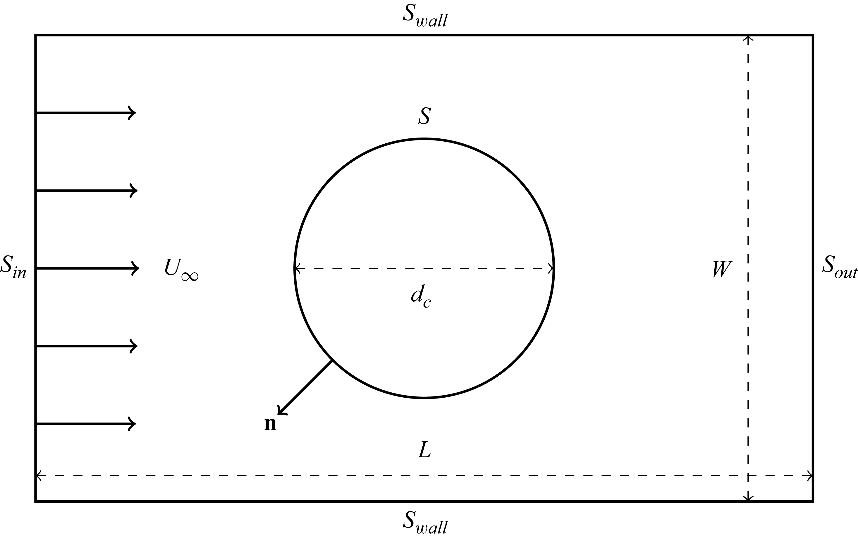
 Sin
 Sout
 Swall
 S
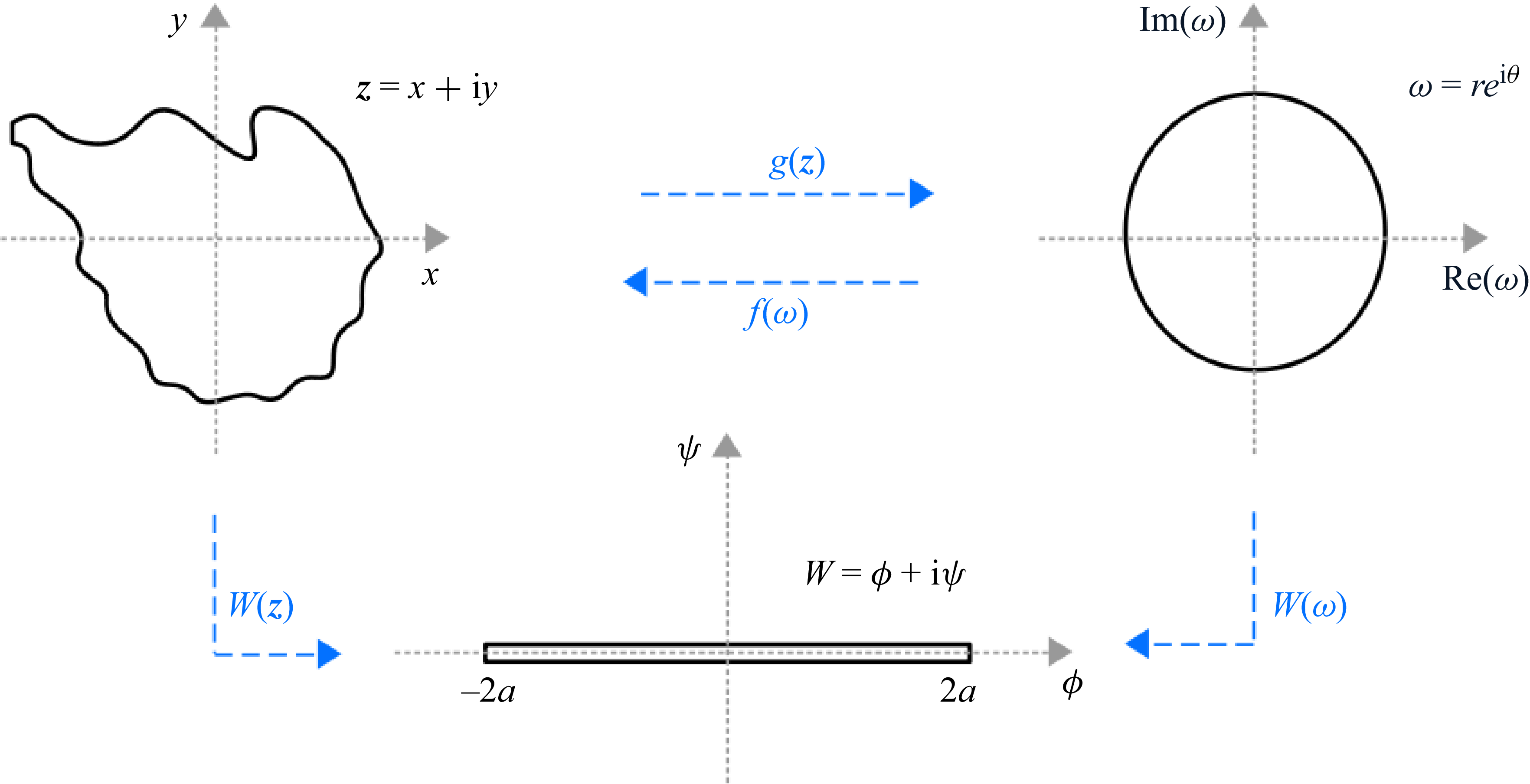
 z
 ω=g(z)
 ω
 z=f(ω)
 W=ϕ+iψ
 W=a(ω+ω−1)
 a
 Rc

 Δx
 a2
 t/tc
 Da→∞
 Da→∞
 Da=66.7
 Da=66.7
 38×33mm2
 Da=66.7
 38×33×0.5mm3
 a=1
 0%
 Da→∞
 Da=66.7

 tc0
 tcnum
 M=32

 tc1
 tc
 tcnum
 M=32

 A/A0

 a
 t/tc
 tc
 log(Da/Pe)
 b0
 tc
 Da/Pe
 log(Pe)
 Ar
 t/tc
 log(Da/Pe)
 Da/Pe
 log(Pe)

 Da=Pe
 Pe=1
 a=0.25
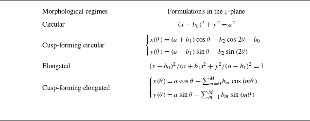
 z

 a¯
 b¯m≤3
 10−2

 ⟨Edef⟩
 Da
 Pe
 Edef¯
 t/tc

 t/tc
 Ar¯
 A/A0¯
 b0¯
 −dA/dt¯

 t/tc

 Da
 Da=Pe/200
 Da=Pe/2
 Pe=50
 Pe=0.8

 a=1
 Pe=0.55
 Da→∞
 q1=0.3+0.2i
 q2=0.35i
 q1=−0.28+0.2i
 q6=0.1
 b0
 c0
 t/tc
 tc
 ∗
 Δz
 ◼

 Open access

