1 Introduction
Exploring the dynamics of magnetized plasmas in the range of scales extending from the ion to the electron Larmor radii (hereafter denoted
 $\unicode[STIX]{x1D70C}_{i}$
and
 $\unicode[STIX]{x1D70C}_{e}$
respectively) is of great importance in various contexts, including magnetic reconnection (Daughton et al.
Reference Daughton, Roytershteyn, Karimabadi, Yin, Albright, Bergen and Bowers2011; Treumann & Baumjohann Reference Treumann and Baumjohann2013; Zweibel & Yamada Reference Zweibel and Yamada2017) and turbulence in space plasmas such as the solar wind (Sahraoui et al.
Reference Sahraoui, Goldstein, Belmont, Canu and Rezeau2010, Reference Sahraoui, Huang, Belmont, Goldstein, Rétino, Robert and De Patoul2013; Matteini et al.
Reference Matteini, Alexandrova, Chen and Lacombe2017) or the auroral regions (Chaston et al.
Reference Chaston, Salem, Bonnell, Carlson, Ergun, Strangeway and McFadden2008). At scales comparable to or smaller than the electron inertial length
 $d_{e}$
, electron inertia cannot be neglected, while electron finite Larmor radius (FLR) corrections play a role at scales approaching
 $\unicode[STIX]{x1D70C}_{e}$
. Although a fully kinetic approach is a priori required to describe plasma dynamics at these scales, ‘reduced fluid models’ can provide an interesting insight when considering relatively small fluctuations about a Maxwellian equilibrium state. Up to the assumptions needed to close the fluid hierarchy, such models can indeed be obtained using systematic asymptotic expansions in regimes where nonlinearities are small and characteristic length scales appropriately selected in order to permit a rigorous estimate of the non-gyrotropic components of the pressure tensor. At scales small compared to
 $\unicode[STIX]{x1D70C}_{i}$
, ions are mostly static, which leads to drastic simplifications. Concerning the electron fluid, two regimes are classically distinguished. Except in the relativistic regimes of large Alfvén velocities (Kuvshinov et al.
Reference Kuvshinov, Westerhof, Schep and Berning1998), this fluid can be viewed as incompressible in the case of whistler waves (WWs). This assumption is in particular usual in electron magnetohydrodynamics (EMHD), a limit of a multifluid description in which the motion of the ions is neglected and the Hall term dominates in the Ohm’s law (see e.g. Kingsep, Chukbar & Yan’kov (Reference Kingsep, Chukbar and Yan’kov1990) or Bulanov, Pegoraro & Sakharov (Reference Bulanov, Pegoraro and Sakharov1992)). If the equilibrium plasma density is uniform, quasi-neutrality then indeed implies incompressibility of the electron flow. Differently, kinetic Alfvén waves (KAWs) are compressible at the sub-ion scales, with pressure fluctuations governed by the perpendicular pressure balance, a description valid as long as their frequency
 $w$
satisfies
 $\unicode[STIX]{x1D714}\ll k_{\bot }v_{thi}$
where
 $v_{thi}$
is the ion thermal velocity and
 $k_{\bot }$
the perpendicular wavenumber, leading to the electron reduced magnetohydrodynamics (ERMHD) (see Schekochihin et al. (Reference Schekochihin, Cowley, Dorland, Hammett, Howes, Quataert and Tatsuno2009) for a review). The electron gyroviscous stress tensor is negligible at scales large compared to
 $\unicode[STIX]{x1D70C}_{e}$
but, except in the case of very large values of the ion to electron temperature ratio
 $\unicode[STIX]{x1D70F}$
, this condition strongly constrains the validity range when scales are also supposed to be small compared to
 $\unicode[STIX]{x1D70C}_{i}$
. This point is exemplified in Tassi, Sulem & Passot (Reference Tassi, Sulem and Passot2016), where comparison with the kinetic theory shows that, in the linear regime, the accuracy of the fluid model for KAWs with
 $\unicode[STIX]{x1D70F}$
and the electron beta parameter
 $\unicode[STIX]{x1D6FD}_{e}$
of order unity, is limited to scales such that
 $k_{\bot }\unicode[STIX]{x1D70C}_{s}\simeq 15$
(here,
 $\unicode[STIX]{x1D70C}_{s}=(m_{i}/2m_{e})^{1/2}\unicode[STIX]{x1D70C}_{e}$
is the sonic Larmor radius with
 $m_{i}$
and
 $m_{e}$
refering to the mass of the ion and of the electron respectively). At smaller scales, non-gyrotropic pressure contributions are to be retained. Their calculation is performed perturbatively in appendix A, when the coupling to the non-gyrotropic part of the heat flux is not retained.
In the sub-ion range, the electron inertial length
 $d_{e}=(2m_{e}/m_{i}\unicode[STIX]{x1D6FD}_{e})^{1/2}\unicode[STIX]{x1D70C}_{s}$
plays an important role as dispersive properties of KAWs and WWs display a qualitative change across this characteristic scale, thus potentially affecting turbulent cascades. In order to study scales smaller than
 $d_{e}$
, but still larger than
 $\unicode[STIX]{x1D70C}_{e}$
, the parameter
 $\unicode[STIX]{x1D6FD}_{e}$
should be taken small. When assuming
 $\unicode[STIX]{x1D6FD}_{e}=O(m_{e}/m_{i})$
as in Zocco & Schekochihin (Reference Zocco and Schekochihin2011), electron inertia should be retained, but electron FLR corrections can be neglected, except for
 $\unicode[STIX]{x1D6FD}_{e}$
-independent terms involved in gyroviscous cancellation. For values of
 $\unicode[STIX]{x1D6FD}_{e}$
that, although small compared to unity, exceed
 $m_{e}/m_{i}$
, the electron gyroviscous force becomes relevant, and it turns out that its computation to order
 $\unicode[STIX]{x1D6FD}_{e}$
at scales comparable to
 $d_{e}$
requires the expansion to be pushed to second order in the scale separation.
The resulting equations for the electrostatic and the parallel magnetic potentials must be supplemented by conditions concerning density and temperature fluctuations. As already mentioned, neglecting density fluctuations or prescribing perpendicular pressure balance leads to discriminate between WWs and KAWs. Concerning temperature fluctuations, we have considered two different regimes. The first one assumes isothermal electrons, which leads to two-field models. Beyond its simplicity, such an assumption appears realistic for turbulent applications when not addressing questions related to plasma heating, and preferable to an adiabatic assumption (Tassi et al. Reference Tassi, Sulem and Passot2016). Temperature indeed tends to be homogenized along the magnetic field lines which, in a turbulent regime, are expected to be stochastic (Schekochihin et al. Reference Schekochihin, Cowley, Dorland, Hammett, Howes, Quataert and Tatsuno2009). A more elaborate model retains dynamical equations for the temperatures and involves a Landau fluid closure to express the gyrotropic heat fluxes, in terms of lower-order moments, in a way consistent with the linear kinetic theory (Hammett & Perkins Reference Hammett and Perkins1990; Snyder, Hammett & Dorland Reference Snyder, Hammett and Dorland1997). As discussed by Hesse, Kuznetsova & Birn (Reference Hesse, Kuznetsova and Birn2004), retaining electron heat fluxes can be an important issue in guide-field magnetic reconnection. The models derived in this paper could indeed be most useful to address questions such as the role of electron pressure anisotropy, Landau damping and FLR corrections in collisionless reconnection, the prevalence of KAWs or WWs depending on the strength of the guiding field, as discussed by Rogers et al. (Reference Rogers, Denton, Drake and Shay2001) (see also Treumann & Baumjohann Reference Treumann and Baumjohann2013).
Being three-dimensional, the reduced fluid models are also well adapted to study turbulence dynamics at sub-ion scales. The regime at scales smaller than
 $d_{e}$
has been extensively studied mostly for WWs, in the framework of EMHD (Biskamp, Schwarz & Drake Reference Biskamp, Schwarz and Drake1996; Biskamp et al.
Reference Biskamp, Schwarz, Zeiler, Celani and Drake1999; Galtier & Bhattacharjee Reference Galtier and Bhattacharjee2003; Lyutikov Reference Lyutikov2013; Galtier & Meyrand Reference Galtier and Meyrand2015), of an incompressible bi-fluid model (Andrés et al.
Reference Andrés, Gonzalez, Martin, Dmitruk and Gómez2014; Andrés, Galtier & Sahraoui Reference Andrés, Galtier and Sahraoui2016a
; Andrés et al.
Reference Andrés, Mininni, Dmitruk and Gómez2016b
) and of extended magnetohydrodynamics (XMHD) (Miloshevich, Lingam & Morrison Reference Miloshevich, Lingam and Morrison2017). Full particle-in-cell simulations of this regime were performed by Gary, Chang & Wang (Reference Gary, Chang and Wang2012) and Chang, Gary & Wang (Reference Chang, Gary and Wang2013). A purpose of the present paper is to address the KAWs dynamics at scales smaller than the electron inertial length, where new regimes of strong and weak turbulence are phenomenologically studied. Due to the compressibility of these waves, magnetic spectra steeper than in the case of WWs are obtained for moderate values of
 $\unicode[STIX]{x1D70F}$
, a property that it could be of interest to compare to the fast-decaying spectra observed in the terrestrial magnetosheath (Huang et al.
Reference Huang, Sahraoui, Deng, He, Yuan, Zhou, Pang and Fu2014).
The paper is organized as follows. Sections 2–4 provide a derivation of reduced models for KAWs and WWs, including the non-gyrotropic electron pressure force, whose calculation is presented in appendix A. Comparisons with previous estimates are made in appendix B. In § 5, closed systems of equations resulting from the assumption of isothermal electrons or from a Landau fluid closure are presented, both in the KAWs and WWs regimes. In § 6, accuracy of these two closures is checked against kinetic theory in the linear regime. In § 7, the isothermal models are used as a basis for a phenomenological theory of KAWs and WWs turbulent cascades, at scales either large or small compared with the electron inertial length. The influence of the ion to electron temperature ratio
 $\unicode[STIX]{x1D70F}$
on the small-scale KAWs spectral exponent is in particular discussed. Section 8 is the conclusion.
2 Reduced form of the Faraday equation
We consider the Faraday equation for the magnetic field
 $\boldsymbol{B}$
 $$\begin{eqnarray}\unicode[STIX]{x2202}_{t}\boldsymbol{B}=-c\unicode[STIX]{x1D735}\times \boldsymbol{E},\end{eqnarray}$$
where the electric field
 $\boldsymbol{E}$
is given by the generalized Ohm’s law
 $$\begin{eqnarray}\boldsymbol{E}=-\frac{1}{c}\boldsymbol{u}_{e}\times \boldsymbol{B}-\frac{1}{en}\unicode[STIX]{x1D735}\boldsymbol{\cdot }\unicode[STIX]{x1D64B}_{e}-\frac{m_{e}}{e}\frac{\text{D}^{(e)}}{\text{D}t}\boldsymbol{u}_{e}.\end{eqnarray}$$
Here
 $c$
is the speed of light,
 $e$
the electron charge and
 $\text{D}^{(e)}/\text{D}t=\unicode[STIX]{x2202}_{t}+\boldsymbol{u}_{e}\boldsymbol{\cdot }\unicode[STIX]{x1D735}$
holds for the material derivative associated with the electron velocity field
 $\boldsymbol{u}_{e}$
. The electron pressure tensor
 $\unicode[STIX]{x1D64B}_{e}$
is given by
 $$\begin{eqnarray}\unicode[STIX]{x1D64B}_{e}=p_{\bot e}\unicode[STIX]{x1D644}+(p_{\Vert e}-p_{\bot e})\unicode[STIX]{x1D749}+\unicode[STIX]{x1D72B}_{e},\end{eqnarray}$$
where
 $\unicode[STIX]{x1D644}$
is the identity matrix,
 $\unicode[STIX]{x1D749}=\widehat{\boldsymbol{b}}\otimes \widehat{\boldsymbol{b}}$
(with
 $\widehat{\boldsymbol{b}}=\boldsymbol{B}/|\boldsymbol{B}|$
),
 $p_{\Vert e}$
and
 $p_{\bot e}$
are the gyrotropic parallel and perpendicular electron pressures and
 $\unicode[STIX]{x1D72B}_{e}$
refers to the FLR contribution to the electron pressure tensor. As usual,
 $n$
holds for the electron number density.
The equation for the parallel magnetic fluctuations
 $B_{z}$
thus reads
 $$\begin{eqnarray}\frac{\text{D}^{(e)}}{\text{D}t}B_{z}+(\unicode[STIX]{x1D735}\boldsymbol{\cdot }\boldsymbol{u}_{e})B_{z}-(\boldsymbol{B}\boldsymbol{\cdot }\unicode[STIX]{x1D735})u_{ze}-\widehat{\boldsymbol{z}}\boldsymbol{\cdot }\unicode[STIX]{x1D735}\times \left(\frac{c}{ne}\unicode[STIX]{x1D735}\boldsymbol{\cdot }\unicode[STIX]{x1D64B}_{e}\right)-\frac{m_{e}c}{e}\widehat{\boldsymbol{z}}\boldsymbol{\cdot }\unicode[STIX]{x1D735}\times \frac{\text{D}^{(e)}}{\text{D}t}\boldsymbol{u}_{e}=0,\end{eqnarray}$$
where
 $\widehat{\boldsymbol{z}}$
denotes the unit vector along the ambient magnetic field. The divergence of the electron velocity is given by the continuity equation
 $$\begin{eqnarray}\unicode[STIX]{x1D735}\boldsymbol{\cdot }\boldsymbol{u}_{e}=-\frac{1}{n}\frac{\text{D}^{(e)}}{\text{D}t}n.\end{eqnarray}$$
In terms of the electrostatic potential
 $\unicode[STIX]{x1D711}$
and of the magnetic potential
 $\boldsymbol{A}$
, defined by
 $\boldsymbol{B}=\unicode[STIX]{x1D735}\times \boldsymbol{A}$
, with the Coulomb gauge
 $\unicode[STIX]{x1D735}\boldsymbol{\cdot }\boldsymbol{A}=0$
, equation (2.1) rewrites
 $$\begin{eqnarray}\boldsymbol{E}=-\unicode[STIX]{x1D735}\unicode[STIX]{x1D711}-\frac{1}{c}\unicode[STIX]{x2202}_{t}\boldsymbol{A}.\end{eqnarray}$$
In addition, when concentrating on sub-ion scales where the electron velocity strongly exceeds that of the ions, the Ampère equation
 $$\begin{eqnarray}\unicode[STIX]{x1D735}\times \boldsymbol{B}=\frac{4\unicode[STIX]{x03C0}}{c}en(\boldsymbol{u}_{i}-\boldsymbol{u}_{e}),\end{eqnarray}$$
where the displacement current is neglected, reduces to
 $$\begin{eqnarray}\boldsymbol{u}_{e}=\frac{c}{4\unicode[STIX]{x03C0}en}\unicode[STIX]{x0394}\boldsymbol{A}.\end{eqnarray}$$
We consider in the following fluctuations about a homogeneous equilibrium state characterized by a number density
 $n_{0}$
, isotropic ion and electron temperatures
 $T_{i0}$
and
 $T_{e0}$
and a guide (or ambient) field of magnitude
 $B_{0}$
taken in the
 $z$
-direction. In order to deal with dimensionless quantities, we rescale time by the inverse ion gyrofrequency
 $\unicode[STIX]{x1D6FA}_{i}=eB_{0}/(m_{i}c)$
, velocities by the sound speed
 $c_{s}=(T_{e0}/m_{i})^{1/2}$
, space coordinates by the sonic Larmor radius
 $\unicode[STIX]{x1D70C}_{s}=c_{s}/\unicode[STIX]{x1D6FA}_{i}$
, density by the equilibrium density
 $n_{0}$
, magnetic field by the equilibrium field
 $B_{0}$
, electric potential by
 $T_{e0}/e$
, parallel magnetic potential by
 $B_{0}\unicode[STIX]{x1D70C}_{s}$
, ion pressures by
 $n_{0}T_{i0}$
, electron pressures by
 $n_{0}T_{e0}$
, parallel and perpendicular electron heat fluxes by
 $c_{s}n_{0}T_{e0}$
and fourth-rank moments by
 $n_{0}T_{e0}^{2}/m_{e}$
. For convenience, we keep the same notation for the rescaled fields. We also define the non-dimensional parameters
 $\unicode[STIX]{x1D70F}=T_{i0}/T_{e0}$
,
 $\unicode[STIX]{x1D6FF}=\sqrt{m_{e}/m_{i}}$
and
 $\unicode[STIX]{x1D6FD}_{e}=8\unicode[STIX]{x03C0}n_{0}T_{e0}/B_{0}^{2}$
.
For a given vector
 $\boldsymbol{V}$
, we denote by
 $V_{\Vert }$
and
 $\boldsymbol{V}_{\bot }$
the components parallel and perpendicular to the local magnetic field (except for the magnetic field, for which
 $\boldsymbol{B}_{\bot }$
refers to the component perpendicular to the ambient field). When the magnetic field distortions are small,
 $V_{\Vert }=V_{z}$
to leading order, except when
 $\boldsymbol{V}$
is quasi-perpendicular (as it is the case for the electric field and also for the gradient operator).
We assume a weakly nonlinear regime characterized by two small parameters
 $\unicode[STIX]{x1D700}$
and
 $\unicode[STIX]{x1D707}$
such that
 $u_{\bot e}=O(\unicode[STIX]{x1D700})$
and
 $\unicode[STIX]{x1D735}_{\bot }=O(1/\unicode[STIX]{x1D707})$
. We furthermore assume that the parallel (
 $\unicode[STIX]{x1D6FB}_{\Vert }=\widehat{\boldsymbol{b}}\boldsymbol{\cdot }\unicode[STIX]{x1D735}$
) and perpendicular (
 $\unicode[STIX]{x1D735}_{\bot }$
) gradients with respect to the local magnetic field satisfy
 $\unicode[STIX]{x1D6FB}_{\Vert }\ll \unicode[STIX]{x1D735}_{\bot }$
, with scalings depending on the type of wave, as specified below. In this asymptotics,
 $\unicode[STIX]{x1D6FB}_{\Vert }=\unicode[STIX]{x2202}_{z}-[A_{\Vert },\cdot ]$
, where the bracket of two scalar functions
 $f$
and
 $g$
is defined as
 $[f,g]=\widehat{\boldsymbol{z}}\boldsymbol{\cdot }(\unicode[STIX]{x1D735}f\times \unicode[STIX]{x1D735}g)$
. Concentrating on scales around
 $d_{e}$
leads us to assume
 $\unicode[STIX]{x1D6FF}^{2}/(\unicode[STIX]{x1D6FD}_{e}\unicode[STIX]{x1D707}^{2})=1$
. At these scales, the condition (in dimensional units)
 $k_{\bot }\unicode[STIX]{x1D70C}_{e}\ll 1$
reduces to
 $\unicode[STIX]{x1D6FD}_{e}\ll 1$
.
We here consider KAWs and WWs. Based on their dispersion relations, we are led to prescribe that for both kinds of waves,
 $\unicode[STIX]{x2202}_{t}=O(\unicode[STIX]{x1D700}/\unicode[STIX]{x1D707})$
,
 $\unicode[STIX]{x1D711}=O(\unicode[STIX]{x1D707}\unicode[STIX]{x1D700})$
,
 $B_{z}=O(\unicode[STIX]{x1D6FD}_{e}\unicode[STIX]{x1D707}\unicode[STIX]{x1D700})$
. Differently, we have
 $\unicode[STIX]{x1D6FB}_{\Vert }=O(\unicode[STIX]{x1D6FF}\unicode[STIX]{x1D700}/\unicode[STIX]{x1D707})=O(\unicode[STIX]{x1D6FD}_{e}^{1/2}\unicode[STIX]{x1D700})$
,
 $A_{\Vert }=O(\unicode[STIX]{x1D6FF}\unicode[STIX]{x1D707}\unicode[STIX]{x1D700})=O(\unicode[STIX]{x1D6FD}_{e}^{-1/2}\unicode[STIX]{x1D6FF}^{2}\unicode[STIX]{x1D700})$
and
 $u_{\Vert e}=O(\unicode[STIX]{x1D707}\unicode[STIX]{x1D700}/\unicode[STIX]{x1D6FF})=O(\unicode[STIX]{x1D6FD}_{e}^{-1/2}\unicode[STIX]{x1D700})$
for the KAWs, while for the WWs,
 $\unicode[STIX]{x1D6FB}_{\Vert }=O(\unicode[STIX]{x1D6FD}_{e}\unicode[STIX]{x1D700})$
,
 $A_{\Vert }=O(\unicode[STIX]{x1D6FD}_{e}\unicode[STIX]{x1D707}^{2}\unicode[STIX]{x1D700})=O(\unicode[STIX]{x1D6FF}^{2}\unicode[STIX]{x1D700})$
and
 $u_{\Vert e}=O(\unicode[STIX]{x1D700})$
. Furthermore,
 $B_{z}/|\boldsymbol{B}_{\bot }|=O(\unicode[STIX]{x1D6FD}_{e}^{1/2})$
for the KAWs, but is of order unity for the WWs (a condition which is not inconsistent with the Coulomb gauge, since
 $|\boldsymbol{A}_{\bot }|$
and
 $A_{\Vert }$
can be comparable when the angle between
 $\boldsymbol{A}_{\bot }$
and
 $\boldsymbol{k}_{\bot }$
is close to
 $\unicode[STIX]{x03C0}/2$
). Similarly, the density, pressure and temperature fluctuations are
 $O(\unicode[STIX]{x1D707}\unicode[STIX]{x1D700})$
for the KAWs, while for the WWs the density fluctuations are negligible and the temperature fluctuations are
 $O(\unicode[STIX]{x1D6FD}_{e}\unicode[STIX]{x1D700}\unicode[STIX]{x1D707})$
. For both types of waves, the gyrotropic heat fluxes
 $q_{\Vert e}$
and
 $q_{\bot e}$
scale like the parallel velocity
 $u_{\Vert e}$
and the fourth-rank cumulants like the temperature fluctuations.
Under the above assumptions, a drift expansion of the transverse electron velocity gives (in terms of the rescaled variables)
 $$\begin{eqnarray}\boldsymbol{u}_{\bot e}=\widehat{\boldsymbol{z}}\times (\unicode[STIX]{x1D735}_{\bot }(\unicode[STIX]{x1D711}-p_{\bot e})-\unicode[STIX]{x1D735}\boldsymbol{\cdot }\unicode[STIX]{x1D72B}_{e}),\end{eqnarray}$$
where, to leading order (see appendix A),
 $\unicode[STIX]{x1D735}\boldsymbol{\cdot }\unicode[STIX]{x1D72B}_{e}=(\unicode[STIX]{x1D6FF}^{2}/2)\unicode[STIX]{x1D735}\unicode[STIX]{x1D714}_{ze}$
, in terms of the parallel electron vorticity
 $\unicode[STIX]{x1D714}_{ze}$
. We write
 $$\begin{eqnarray}\boldsymbol{u}_{\bot e}=\widehat{\boldsymbol{z}}\times \unicode[STIX]{x1D735}_{\bot }\unicode[STIX]{x1D711}^{\ast },\end{eqnarray}$$
with
 $$\begin{eqnarray}\unicode[STIX]{x1D711}^{\ast }=\unicode[STIX]{x1D711}-p_{\bot e}-\frac{\unicode[STIX]{x1D6FF}^{2}}{2}\unicode[STIX]{x1D714}_{ze}.\end{eqnarray}$$
In (2.11) and hereafter, the various fields refer to fluctuations, except for the pressure in primitive equations.
Furthermore, using (2.8),
 $$\begin{eqnarray}\displaystyle & \displaystyle u_{\Vert e}=\frac{2}{\unicode[STIX]{x1D6FD}_{e}}\unicode[STIX]{x1D6E5}_{\bot }A_{\Vert } & \displaystyle\end{eqnarray}$$
 $$\begin{eqnarray}\displaystyle & \displaystyle \unicode[STIX]{x1D714}_{ze}=\unicode[STIX]{x1D6E5}_{\bot }\unicode[STIX]{x1D711}^{\ast } & \displaystyle\end{eqnarray}$$
 $$\begin{eqnarray}\displaystyle & \displaystyle \unicode[STIX]{x1D711}^{\ast }=\frac{2}{\unicode[STIX]{x1D6FD}_{e}}B_{z} & \displaystyle\end{eqnarray}$$
 $$\begin{eqnarray}\displaystyle & \displaystyle \left(1+\frac{\unicode[STIX]{x1D6FF}^{2}}{2}\unicode[STIX]{x1D6E5}_{\bot }\right)\unicode[STIX]{x1D711}^{\ast }=\unicode[STIX]{x1D711}-p_{\bot e}. & \displaystyle\end{eqnarray}$$
It follows that
 $$\begin{eqnarray}\frac{\text{D}^{(e)}}{\text{D}t}=\frac{\text{d}}{\text{d}t}-\left[p_{\bot e}+\frac{\unicode[STIX]{x1D6FF}^{2}}{\unicode[STIX]{x1D6FD}_{e}}\unicode[STIX]{x1D6E5}_{\bot }B_{z},\boldsymbol{\cdot }\right],\end{eqnarray}$$
where
 $\text{d}/\text{d}t=\unicode[STIX]{x2202}_{t}+[\unicode[STIX]{x1D711},\boldsymbol{\cdot }]$
.
The projection on the parallel direction of (2.6),
 $$\begin{eqnarray}\unicode[STIX]{x2202}_{t}A_{\Vert }+c\unicode[STIX]{x1D6FB}_{\Vert }\unicode[STIX]{x1D711}=-cE_{\Vert },\end{eqnarray}$$
rewrites
 $$\begin{eqnarray}\frac{\text{d}}{\text{d}t}\left(1-\frac{2\unicode[STIX]{x1D6FF}^{2}}{\unicode[STIX]{x1D6FD}_{e}}\unicode[STIX]{x1D6E5}_{\bot }\right)A_{\Vert }+\unicode[STIX]{x2202}_{z}\unicode[STIX]{x1D711}-\unicode[STIX]{x1D6FB}_{\Vert }p_{\Vert e}+\unicode[STIX]{x1D6FF}^{2}\left[p_{\bot e}+\frac{\unicode[STIX]{x1D6FF}^{2}}{2}\unicode[STIX]{x1D714}_{ze},u_{\Vert e}\right]-\widehat{\boldsymbol{b}}\boldsymbol{\cdot }(\unicode[STIX]{x1D735}\boldsymbol{\cdot }\unicode[STIX]{x1D72B}_{e})=0,\end{eqnarray}$$
where the FLR contributions
 $\widehat{\boldsymbol{b}}\boldsymbol{\cdot }(\unicode[STIX]{x1D735}\boldsymbol{\cdot }\unicode[STIX]{x1D72B}_{e})=\widehat{\boldsymbol{b}}\boldsymbol{\cdot }\unicode[STIX]{x1D735}\boldsymbol{\cdot }\unicode[STIX]{x1D72B}_{e}^{(1)}+\widehat{\boldsymbol{b}}\boldsymbol{\cdot }\unicode[STIX]{x1D735}\boldsymbol{\cdot }\unicode[STIX]{x1D72B}_{e}^{(2)}$
are given by (A 8), (A 9), (A 11) and (A 19). Equation (2.18) rewrites
 $$\begin{eqnarray}\displaystyle & & \displaystyle \frac{\text{d}}{\text{d}t}\left(1-\frac{2\unicode[STIX]{x1D6FF}^{2}}{\unicode[STIX]{x1D6FD}_{e}}\unicode[STIX]{x1D6E5}_{\bot }+\frac{2\unicode[STIX]{x1D6FF}^{4}}{\unicode[STIX]{x1D6FD}_{e}}\unicode[STIX]{x1D6E5}_{\bot }^{2}\right)A_{\Vert }+\unicode[STIX]{x2202}_{z}\unicode[STIX]{x1D711}-\unicode[STIX]{x1D6FB}_{\Vert }p_{\Vert e}-\left[p_{\bot e},\frac{2\unicode[STIX]{x1D6FF}^{4}}{\unicode[STIX]{x1D6FD}_{e}}\unicode[STIX]{x1D6E5}_{\bot }^{2}A_{\Vert }\right]\nonumber\\ \displaystyle & & \displaystyle \quad +\,\unicode[STIX]{x1D6FF}^{2}[B_{z},u_{\Vert e}+q_{\bot e}]-\unicode[STIX]{x1D6FF}^{2}\unicode[STIX]{x1D6FB}_{\Vert }\unicode[STIX]{x1D6E5}_{\bot }\unicode[STIX]{x1D711}^{\ast }-\unicode[STIX]{x1D6FF}^{2}\mathop{\sum }_{i=x,y}\left[\unicode[STIX]{x2202}_{i}\unicode[STIX]{x1D711}^{\ast },\left(1-\frac{2\unicode[STIX]{x1D6FF}^{2}}{\unicode[STIX]{x1D6FD}_{e}}\unicode[STIX]{x1D6E5}_{\bot }\right)\unicode[STIX]{x2202}_{i}A_{\Vert }\right]\nonumber\\ \displaystyle & & \displaystyle \quad +\,\unicode[STIX]{x1D6FF}^{4}\frac{\text{d}}{\text{d}t}\unicode[STIX]{x1D6E5}_{\bot }q_{\bot e}-\unicode[STIX]{x1D6FF}^{4}[p_{\bot e},\unicode[STIX]{x1D6E5}_{\bot }q_{\bot e}]-\unicode[STIX]{x1D6FF}^{4}[\unicode[STIX]{x1D6E5}_{\bot }\unicode[STIX]{x1D711}^{\ast },q_{\bot e}]=0,\end{eqnarray}$$
where the gyroviscous cancellation eliminates the
 $\unicode[STIX]{x1D6FF}^{2}[p_{\bot e}+(\unicode[STIX]{x1D6FF}^{2}/2)\unicode[STIX]{x1D714}_{ze},u_{\Vert e}]$
term.
We now turn to (2.4) where, assuming an isotropic equilibrium state, we write
 $$\begin{eqnarray}\unicode[STIX]{x1D735}\boldsymbol{\cdot }\unicode[STIX]{x1D64B}_{e}=\unicode[STIX]{x1D6FB}_{\bot }p_{\bot e}+\unicode[STIX]{x1D6FB}_{\Vert }p_{\Vert e}\widehat{\boldsymbol{b}}+\unicode[STIX]{x1D735}\boldsymbol{\cdot }\unicode[STIX]{x1D72B}_{e}.\end{eqnarray}$$
At the order of the present expansion, we have
 $$\begin{eqnarray}\widehat{\boldsymbol{z}}\boldsymbol{\cdot }\unicode[STIX]{x1D735}\times \frac{\text{D}^{(e)}}{\text{D}t}\boldsymbol{u}_{e}=\frac{\text{D}^{(e)}}{\text{D}t}\unicode[STIX]{x1D714}_{ze}=\frac{2}{\unicode[STIX]{x1D6FD}_{e}}\frac{\text{D}^{(e)}}{\text{D}t}\unicode[STIX]{x1D6E5}_{\bot }B_{z}\end{eqnarray}$$
and
 $$\begin{eqnarray}\displaystyle \widehat{\boldsymbol{z}}\boldsymbol{\cdot }\unicode[STIX]{x1D735}\times (\unicode[STIX]{x1D735}\boldsymbol{\cdot }\unicode[STIX]{x1D72B}_{e}) & = & \displaystyle \frac{2\unicode[STIX]{x1D6FF}^{2}}{\unicode[STIX]{x1D6FD}_{e}}[p_{\bot e}-B_{z},\unicode[STIX]{x1D6E5}_{\bot }B_{z}]+\unicode[STIX]{x1D6FF}^{2}\mathop{\sum }_{i=x,y}[\unicode[STIX]{x2202}_{i}(p_{\bot e}-B_{z}),\unicode[STIX]{x2202}_{i}\unicode[STIX]{x1D711}^{\ast }]\nonumber\\ \displaystyle & & \displaystyle -\,\frac{\unicode[STIX]{x1D6FF}^{2}}{2}\unicode[STIX]{x1D6E5}_{\bot }\unicode[STIX]{x1D735}\boldsymbol{\cdot }\boldsymbol{u}_{e}-\frac{\unicode[STIX]{x1D6FF}^{2}}{2}\unicode[STIX]{x1D6FB}_{\Vert }\unicode[STIX]{x1D6E5}_{\bot }u_{\Vert e}-\unicode[STIX]{x1D6FF}^{2}\unicode[STIX]{x1D6FB}_{\Vert }\unicode[STIX]{x1D6E5}_{\bot }q_{\bot e}+\unicode[STIX]{x1D6FF}^{2}\mathop{\sum }_{i=x,y}[\unicode[STIX]{x2202}_{i}A_{\Vert },\unicode[STIX]{x2202}_{i}q_{\bot e}].\nonumber\\ \displaystyle & & \displaystyle\end{eqnarray}$$
Using (A 22), we obtain
 $$\begin{eqnarray}\displaystyle & & \displaystyle \frac{\text{d}}{\text{d}t}\left(\left(1-\frac{2\unicode[STIX]{x1D6FF}^{2}}{\unicode[STIX]{x1D6FD}_{e}}\unicode[STIX]{x1D6E5}_{\bot }\right)B_{z}\right)-\left[p_{\bot e}+\frac{\unicode[STIX]{x1D6FF}^{2}}{\unicode[STIX]{x1D6FD}_{e}}\unicode[STIX]{x1D6E5}_{\bot }B_{z},B_{z}+n\right]+\left(1+\frac{\unicode[STIX]{x1D6FF}^{2}}{2}\unicode[STIX]{x1D6E5}_{\bot }\right)(\unicode[STIX]{x1D735}\boldsymbol{\cdot }\boldsymbol{u}_{e})\nonumber\\ \displaystyle & & \displaystyle \quad -\,\unicode[STIX]{x1D6FB}_{\Vert }\left(1-\frac{\unicode[STIX]{x1D6FF}^{2}}{2}\unicode[STIX]{x1D6E5}_{\bot }\right)u_{\Vert e}+\unicode[STIX]{x1D6FF}^{2}[B_{z},\unicode[STIX]{x1D6E5}_{\bot }\unicode[STIX]{x1D711}^{\ast }]-\unicode[STIX]{x1D6FF}^{2}\mathop{\sum }_{i=x,y}[\unicode[STIX]{x2202}_{i}p_{\bot e},\unicode[STIX]{x2202}_{i}\unicode[STIX]{x1D711}^{\ast }]\nonumber\\ \displaystyle & & \displaystyle \quad +\,\unicode[STIX]{x1D6FF}^{2}\unicode[STIX]{x1D6FB}_{\Vert }\unicode[STIX]{x1D6E5}_{\bot }q_{\bot e}-\unicode[STIX]{x1D6FF}^{2}\mathop{\sum }_{i=x,y}[\unicode[STIX]{x2202}_{i}A_{\Vert },\unicode[STIX]{x2202}_{i}q_{\bot e}]=0\end{eqnarray}$$
or, when using (2.5),
 $$\begin{eqnarray}\displaystyle & & \displaystyle \frac{\text{d}}{\text{d}t}\left(\left(1-\frac{2\unicode[STIX]{x1D6FF}^{2}}{\unicode[STIX]{x1D6FD}_{e}}\unicode[STIX]{x1D6E5}_{\bot }\right)B_{z}-\left(1+\frac{\unicode[STIX]{x1D6FF}^{2}}{2}\unicode[STIX]{x1D6E5}_{\bot }\right)n\right)-\left[p_{\bot e}+\frac{3\unicode[STIX]{x1D6FF}^{2}}{\unicode[STIX]{x1D6FD}_{e}}\unicode[STIX]{x1D6E5}_{\bot }B_{z},B_{z}\right]-\frac{\unicode[STIX]{x1D6FF}^{2}}{2}[\unicode[STIX]{x1D6E5}_{\bot }\unicode[STIX]{x1D711},n]\nonumber\\ \displaystyle & & \displaystyle \quad +\,\frac{\unicode[STIX]{x1D6FF}^{2}}{2}\unicode[STIX]{x1D6E5}_{\bot }\left[p_{\bot e}+\frac{\unicode[STIX]{x1D6FF}^{2}}{\unicode[STIX]{x1D6FD}_{e}}\unicode[STIX]{x1D6E5}_{\bot }B_{z},n\right]-\frac{2}{\unicode[STIX]{x1D6FD}_{e}}\unicode[STIX]{x1D6FB}_{\Vert }\left(1-\frac{\unicode[STIX]{x1D6FF}^{2}}{2}\unicode[STIX]{x1D6E5}_{\bot }\right)\unicode[STIX]{x1D6E5}_{\bot }A_{\Vert }+\unicode[STIX]{x1D6FF}^{2}\mathop{\sum }_{i=x,y}[\unicode[STIX]{x2202}_{i}n,\unicode[STIX]{x2202}_{i}\unicode[STIX]{x1D711}]\nonumber\\ \displaystyle & & \displaystyle \quad -\,\unicode[STIX]{x1D6FF}^{2}[\unicode[STIX]{x2202}_{i}p_{\bot e},\unicode[STIX]{x2202}_{i}\unicode[STIX]{x1D711}^{\ast }]+\unicode[STIX]{x1D6FF}^{2}\unicode[STIX]{x1D6FB}_{\Vert }\unicode[STIX]{x1D6E5}_{\bot }q_{\bot e}-\unicode[STIX]{x1D6FF}^{2}\mathop{\sum }_{i=x,y}[\unicode[STIX]{x2202}_{i}A_{\Vert },\unicode[STIX]{x2202}_{i}q_{\bot e}]=0.\end{eqnarray}$$
3 Pressure equations
The equations for the electron gyrotropic pressures read
 $$\begin{eqnarray}\displaystyle & \!\displaystyle \frac{\text{D}^{(e)}}{\text{D}t}p_{\Vert e}+p_{\Vert e}\unicode[STIX]{x1D735}\boldsymbol{\cdot }\boldsymbol{u}_{e}+2p_{\Vert e}\unicode[STIX]{x1D6FB}_{\Vert }\boldsymbol{u}_{e}\boldsymbol{\cdot }\widehat{\boldsymbol{b}}+\unicode[STIX]{x1D735}\boldsymbol{\cdot }\unicode[STIX]{x1D666}_{e}\boldsymbol{ : }\unicode[STIX]{x1D749}+\left[(\unicode[STIX]{x1D72B}_{e}\boldsymbol{\cdot }\unicode[STIX]{x1D735}\boldsymbol{u}_{e})^{S}\boldsymbol{ : }\unicode[STIX]{x1D749}-\unicode[STIX]{x1D72B}_{e}\boldsymbol{ : }\frac{\text{d}\unicode[STIX]{x1D749}}{\text{d}t}\right]=0 & \displaystyle \nonumber\\ \displaystyle & & \displaystyle\end{eqnarray}$$
 $$\begin{eqnarray}\displaystyle & \!\displaystyle \frac{\text{D}^{(e)}}{\text{D}t}p_{\bot e}+2p_{\bot e}\unicode[STIX]{x1D735}\boldsymbol{\cdot }\boldsymbol{u}_{e}-p_{\bot e}\unicode[STIX]{x1D6FB}_{\Vert }\boldsymbol{u}_{e}\boldsymbol{\cdot }\widehat{\boldsymbol{b}}+\frac{1}{2}\unicode[STIX]{x1D735}\boldsymbol{\cdot }\unicode[STIX]{x1D666}_{e}\boldsymbol{ : }\unicode[STIX]{x1D663}+\frac{1}{2}\left[(\unicode[STIX]{x1D72B}_{e}\boldsymbol{\cdot }\unicode[STIX]{x1D735}\boldsymbol{u}_{e})^{S}\boldsymbol{ : }\unicode[STIX]{x1D663}+\unicode[STIX]{x1D72B}_{e}\boldsymbol{ : }\frac{\text{d}\unicode[STIX]{x1D749}}{\text{d}t}\right]=0, & \displaystyle \nonumber\\ \displaystyle & & \displaystyle\end{eqnarray}$$
where
 $\boldsymbol{n}=\boldsymbol{I}-\unicode[STIX]{x1D749}$
and the electron heat flux tensor
 $\unicode[STIX]{x1D666}_{e}$
can be written
 $\unicode[STIX]{x1D666}_{e}=\unicode[STIX]{x1D64E}_{e}+\unicode[STIX]{x1D748}_{e}$
. Here the tensor
 $\unicode[STIX]{x1D748}_{e}$
obeys the conditions
 $\unicode[STIX]{x1D748}_{e}\boldsymbol{ : }\unicode[STIX]{x1D663}=0$
and
 $\unicode[STIX]{x1D748}_{e}\boldsymbol{ : }\unicode[STIX]{x1D749}=0$
. The elements of the tensor
 $\unicode[STIX]{x1D64E}_{e}$
are classically expressed (see e.g. Goswami, Passot & Sulem Reference Goswami, Passot and Sulem2005) in terms of the components of two vectors
 $\boldsymbol{S}_{e}^{\Vert }$
and
 $\boldsymbol{S}_{e}^{\bot }$
defined by
 $\boldsymbol{S}_{e}^{\Vert }=\unicode[STIX]{x1D666}_{e}\boldsymbol{ : }\unicode[STIX]{x1D749}$
and
 $\boldsymbol{S}_{e}^{\bot }=(1/2)\unicode[STIX]{x1D666}_{e}\boldsymbol{ : }\unicode[STIX]{x1D663}$
that measure the directional fluxes of the parallel and perpendicular heats respectively. The usual perpendicular and parallel gyrotropic heat fluxes are given by
 $q_{\bot e}=\boldsymbol{S}_{e}^{\bot }\boldsymbol{\cdot }\boldsymbol{b}$
and
 $q_{\Vert e}=\boldsymbol{S}_{e}^{\Vert }\boldsymbol{\cdot }\boldsymbol{b}$
, and thus correspond to the fluxes along the magnetic field. We write
 $\boldsymbol{S}_{e}^{\bot }=q_{\bot e}\boldsymbol{b}+\boldsymbol{S}_{\bot e}^{\bot }$
and
 $\boldsymbol{S}_{e}^{\Vert }=q_{\Vert e}\boldsymbol{b}+\boldsymbol{S}_{\bot e}^{\Vert }$
.
In the present asymptotics, the contribution to the pressure equations of the tensor
 $\unicode[STIX]{x1D748}_{e}$
, whose expression, given in Ramos (Reference Ramos2005a
) and also in Sulem & Passot (Reference Sulem and Passot2015), is negligible. To leading order, we are thus led to write
 $$\begin{eqnarray}\displaystyle & (\unicode[STIX]{x1D735}\boldsymbol{\cdot }\boldsymbol{q}_{e})\boldsymbol{ : }\unicode[STIX]{x1D749}=\unicode[STIX]{x1D6FB}_{\Vert }q_{\Vert e}+\unicode[STIX]{x1D735}\boldsymbol{\cdot }\boldsymbol{S}_{\bot e}^{\Vert } & \displaystyle\end{eqnarray}$$
 $$\begin{eqnarray}\displaystyle & \displaystyle {\textstyle \frac{1}{2}}(\unicode[STIX]{x1D735}\boldsymbol{\cdot }\boldsymbol{q}_{e})\boldsymbol{ : }\boldsymbol{n}=\unicode[STIX]{x1D6FB}_{\Vert }q_{\bot e}+\unicode[STIX]{x1D735}\boldsymbol{\cdot }\boldsymbol{S}_{\bot e}^{\bot }. & \displaystyle\end{eqnarray}$$
Here, the non-gyrotropic heat fluxes contributions, described by the vectors
 $\boldsymbol{S}_{\bot e}^{\Vert }$
and
 $\boldsymbol{S}_{\bot e}^{\bot }$
, are obtained by changing sign in the equations (3.6) and (3.7) of Sulem & Passot (Reference Sulem and Passot2015) for the ion heat flux vectors. We obtain, at the order of the asymptotics,
 $$\begin{eqnarray}\displaystyle & \displaystyle \boldsymbol{S}_{\bot e}^{\Vert }=-\frac{1}{B}\widehat{\boldsymbol{b}}\times (p_{\bot e}\unicode[STIX]{x1D735}T_{\Vert e}+2\unicode[STIX]{x1D6FF}^{2}q_{\bot e}\widehat{\boldsymbol{b}}\times \unicode[STIX]{x1D74E}_{e}+\unicode[STIX]{x1D735}\widetilde{r}_{\Vert \bot e}) & \displaystyle\end{eqnarray}$$
 $$\begin{eqnarray}\displaystyle & \displaystyle \boldsymbol{S}_{\bot e}^{\bot }=-\frac{2}{B}\widehat{\boldsymbol{b}}\times (p_{\bot _{e}}\unicode[STIX]{x1D735}T_{\bot e}+\unicode[STIX]{x1D735}\widetilde{r}_{\bot \bot e}), & \displaystyle\end{eqnarray}$$
where the
 $\widetilde{r}$
functions refer to the gyrotropic components of the fourth-rank cumulants.
Among the terms associated with the work of the non-gyrotropic pressure force in (3.1) and (3.2), the one involving the time derivative scales like
 $O(\unicode[STIX]{x1D700}^{3})$
and is thus negligible. In the other terms, only the linear part of
 $\unicode[STIX]{x1D72B}_{e}$
is possibly relevant at the prescribed order, but it is easily checked that the corresponding contribution in fact vanishes.
Using the electron continuity equation to eliminate the velocity divergence, we are led to write the equations for the temperature fluctuations
 $$\begin{eqnarray}\displaystyle & \displaystyle \frac{\text{d}}{\text{d}t}T_{\Vert e}-[B_{z},T_{\Vert e}+\widetilde{r}_{\Vert \bot e}]+\unicode[STIX]{x1D6FB}_{\Vert }(2u_{\Vert e}+q_{\Vert e})-\frac{\unicode[STIX]{x1D6FF}^{2}}{\unicode[STIX]{x1D6FD}_{e}}[\unicode[STIX]{x1D6E5}_{\bot }B_{z},T_{\Vert e}]+2\unicode[STIX]{x1D6FF}^{2}[q_{\bot e},u_{\Vert e}]=0\quad & \displaystyle\end{eqnarray}$$
 $$\begin{eqnarray}\displaystyle & \displaystyle \frac{\text{d}}{\text{d}t}(T_{\bot e}-n)-2[B_{z},T_{\bot e}+\widetilde{r}_{\bot \bot e}]+\unicode[STIX]{x1D6FB}_{\Vert }(q_{\bot e}-u_{\Vert e})-\frac{\unicode[STIX]{x1D6FF}^{2}}{\unicode[STIX]{x1D6FD}_{e}}[\unicode[STIX]{x1D6E5}_{\bot }B_{z},T_{\bot e}-n]=0,\quad & \displaystyle\end{eqnarray}$$
where
 $u_{\Vert e}$
and
 $B_{z}$
are given by (2.12) and (2.14) respectively.
4 KAWs or WWs, depending on the compressibility level
At this stage, it is important to note that, beyond the estimate of the gyrotropic electron pressure fluctuations which are prescribed by the closure assumption for the fluid hierarchy, the system given by (2.19) and (2.24) involves three unknown quantities
 $A_{\Vert }$
,
 $\unicode[STIX]{x1D711}$
and
 $n$
. An additional relation is obtained when specifying the type of waves the system is describing. KAWs and WWs are indeed characterized by different levels of compressibility.
In the case of KAWs, the plasma is in pressure balance in the transverse direction. This condition, which consists in neglecting the inertial term compared to the pressure gradient in the equation for the transverse total momentum reads (for typical ion transverse velocity
 $\unicode[STIX]{x1D6FF}v_{\bot i}$
and density fluctuations
 $\unicode[STIX]{x1D6FF}n$
),
 $$\begin{eqnarray}\frac{\unicode[STIX]{x1D714}}{k_{\bot }}\frac{\unicode[STIX]{x1D6FF}v_{\bot i}}{v_{thi}}\ll v_{thi}\frac{\unicode[STIX]{x1D6FF}n}{n}.\end{eqnarray}$$
In the above estimate, in spite of the fact that
 $|\boldsymbol{u}_{i}|\ll |\boldsymbol{u}_{e}|$
,
 $m_{i}\unicode[STIX]{x1D6FF}v_{\bot i}$
dominates
 $m_{e}\unicode[STIX]{x1D6FF}v_{\bot e}$
, at least close to the ion scale where
 $\unicode[STIX]{x1D6FF}v_{\bot i}/v_{thi}$
and
 $\unicode[STIX]{x1D6FF}n/n$
are comparable, and where one thus recovers the classical condition
 $\unicode[STIX]{x1D714}\ll k_{\bot }v_{thi}$
for the existence of KAWs. At smaller scales, where the ion velocity fluctuations decrease due to ion demagnetization, this condition becomes in fact less stringent. The pressure balance then reads
 $$\begin{eqnarray}(\unicode[STIX]{x1D735}\boldsymbol{\cdot }(\unicode[STIX]{x1D70F}\unicode[STIX]{x1D64B}_{i}+\unicode[STIX]{x1D64B}_{e}))_{\bot }-\frac{2}{\unicode[STIX]{x1D6FD}_{e}}(\unicode[STIX]{x1D735}\times \boldsymbol{B})\times \widehat{\boldsymbol{z}}=0,\end{eqnarray}$$
where the index
 $i$
refers to the ions. Applying the transverse divergence, we find
 $$\begin{eqnarray}\unicode[STIX]{x1D6E5}_{\bot }(\unicode[STIX]{x1D70F}p_{\bot i}+p_{\bot e})+\unicode[STIX]{x1D735}_{\bot }\boldsymbol{\cdot }(\unicode[STIX]{x1D735}\boldsymbol{\cdot }(\unicode[STIX]{x1D70F}\unicode[STIX]{x1D72B}_{i}+\unicode[STIX]{x1D72B}_{e}))+\frac{2}{\unicode[STIX]{x1D6FD}_{e}}\unicode[STIX]{x1D6E5}_{\bot }B_{z}=0.\end{eqnarray}$$
As shown in Tassi et al. (Reference Tassi, Sulem and Passot2016), at the sub-ion scales,
 $\unicode[STIX]{x1D72B}_{i}$
is negligible and the ions are isothermal (making, in the present units, electron pressure and density fluctuations equal). To leading order in
 $\unicode[STIX]{x1D700}$
, equation (4.3) rewrites
 $$\begin{eqnarray}\unicode[STIX]{x1D70F}n+p_{\bot e}+\frac{\unicode[STIX]{x1D6FF}^{2}}{2}\unicode[STIX]{x0394}\unicode[STIX]{x1D711}^{\ast }+\frac{2}{\unicode[STIX]{x1D6FD}_{e}}B_{z}=0.\end{eqnarray}$$
Using (2.14) and (2.15), it is then easily checked that
 $$\begin{eqnarray}n=-\frac{1}{\unicode[STIX]{x1D70F}}\unicode[STIX]{x1D711}.\end{eqnarray}$$
It results that
 $$\begin{eqnarray}\displaystyle & \displaystyle n=-\frac{1}{1+\unicode[STIX]{x1D70F}}\left(T_{\bot e}+\left(1+\frac{\unicode[STIX]{x1D6FF}^{2}}{2}\unicode[STIX]{x1D6E5}_{\bot }\right)\unicode[STIX]{x1D711}^{\ast }\right) & \displaystyle\end{eqnarray}$$
 $$\begin{eqnarray}\displaystyle & \displaystyle \unicode[STIX]{x1D711}=\frac{\unicode[STIX]{x1D70F}}{1+\unicode[STIX]{x1D70F}}\left(T_{\bot e}+\left(1+\frac{\unicode[STIX]{x1D6FF}^{2}}{2}\unicode[STIX]{x1D6E5}_{\bot }\right)\unicode[STIX]{x1D711}^{\ast }\right). & \displaystyle\end{eqnarray}$$
A different behaviour of the density holds in the case of the WWs. The linear kinetic theory (see e.g. Gary & Smith Reference Gary and Smith2009) shows that the electron compressibility of WWs is significantly smaller than that of the KAWs, at least for
 $\unicode[STIX]{x1D6FD}_{e}$
small enough compared to unity and scales small compared to
 $d_{i}$
. This suggests that we may assume
 $\unicode[STIX]{x1D735}\boldsymbol{\cdot }\boldsymbol{u}_{e}$
is smaller than
 $\unicode[STIX]{x1D700}^{2}$
, and thus may neglect the density fluctuations. This regime formally corresponds to taking the limit
 $\unicode[STIX]{x1D70F}\rightarrow \infty$
in (4.6) and (4.7). Note however than in auroral zones where the Alfvén velocity can exceed several thousands of
 $\text{km}~\text{s}^{-1}$
, quasi-neutrality no longer holds at large enough wavenumber, making electron density fluctuations relevant for WW dynamics (Kuvshinov et al.
Reference Kuvshinov, Westerhof, Schep and Berning1998).
In the next section, two different closures of the fluid hierarchy will be examined, namely the isothermal case, a regime often considered in turbulence studies, and a Landau fluid closure.
5 Closure assumptions
5.1 General form of the four-field model
Two asymptotics which are similar but not identical can be distinguished. When considering scales comparable to
 $d_{e}$
, we should take
 $\unicode[STIX]{x1D6FD}_{e}$
as the expansion parameter. We refer in the following to this regime as the small
 $\unicode[STIX]{x1D6FD}_{e}$
regime. Differently, when considering
 $\unicode[STIX]{x1D6FD}_{e}$
of order unity, a gradient expansion is performed in terms of
 $\unicode[STIX]{x1D6FF}^{2}\unicode[STIX]{x1D6E5}_{\bot }$
(hereafter referred to as large-scale regime). In fact both approaches can be captured simultaneously, but this leads us to retain subdominant terms of order
 $\unicode[STIX]{x1D6FD}_{e}\unicode[STIX]{x1D6FF}^{2}\unicode[STIX]{x1D6E5}_{\bot }=O(\unicode[STIX]{x1D6FD}_{e}^{2})$
in the former regime and of order
 $\unicode[STIX]{x1D6FF}^{4}\unicode[STIX]{x1D6E5}_{\bot }^{2}/\unicode[STIX]{x1D6FD}_{e}$
in the latter.
In the KAW regime, using (4.6)–(4.7), equations (2.19) and (2.24) rewrite,
 $$\begin{eqnarray}\displaystyle & & \displaystyle \unicode[STIX]{x2202}_{t}\left(\left(1-\frac{2\unicode[STIX]{x1D6FF}^{2}}{\unicode[STIX]{x1D6FD}_{e}}\unicode[STIX]{x1D6E5}_{\bot }+\frac{2\unicode[STIX]{x1D6FF}^{4}}{\unicode[STIX]{x1D6FD}_{e}}\unicode[STIX]{x1D6E5}_{\bot }^{2}\right)A_{\Vert }+\unicode[STIX]{x1D6FF}^{4}\unicode[STIX]{x1D6E5}_{\bot }q_{\bot e}\right)+\unicode[STIX]{x1D6FB}_{\Vert }(T_{\bot e}-T_{\Vert e})+\unicode[STIX]{x1D6FB}_{\Vert }\left(1-\frac{\unicode[STIX]{x1D6FF}^{2}}{2}\unicode[STIX]{x1D6E5}_{\bot }\right)\unicode[STIX]{x1D711}^{\ast }\nonumber\\ \displaystyle & & \displaystyle \quad +\left[\unicode[STIX]{x1D711}^{\ast },\unicode[STIX]{x1D6FF}^{2}\unicode[STIX]{x1D6E5}_{\bot }A_{\Vert }+\frac{2\unicode[STIX]{x1D6FF}^{4}}{\unicode[STIX]{x1D6FD}_{e}}\unicode[STIX]{x1D6E5}_{\bot }^{2}A_{\Vert }\right]-\frac{\unicode[STIX]{x1D70F}}{1+\unicode[STIX]{x1D70F}}\left[T_{\bot e}+\left(1+\frac{\unicode[STIX]{x1D6FF}^{2}}{2}\unicode[STIX]{x1D6E5}_{\bot }\right)\unicode[STIX]{x1D711}^{\ast },\frac{2\unicode[STIX]{x1D6FF}^{2}}{\unicode[STIX]{x1D6FD}_{e}}\unicode[STIX]{x1D6E5}_{\bot }A_{\Vert }\right]\nonumber\\ \displaystyle & & \displaystyle \quad -\,\unicode[STIX]{x1D6FF}^{2}\mathop{\sum }_{i=x,y}\left[\unicode[STIX]{x2202}_{i}\unicode[STIX]{x1D711}^{\ast },\left(1-\frac{2\unicode[STIX]{x1D6FF}^{2}}{\unicode[STIX]{x1D6FD}_{e}}\unicode[STIX]{x1D6E5}_{\bot }\right)\unicode[STIX]{x2202}_{i}A_{\Vert }\right]+\left[\unicode[STIX]{x1D711}^{\ast },\frac{\unicode[STIX]{x1D6FD}_{e}}{2}\unicode[STIX]{x1D6FF}^{2}q_{\bot e}+\unicode[STIX]{x1D6FF}^{4}\unicode[STIX]{x1D6E5}_{\bot }q_{\bot e}\right]\nonumber\\ \displaystyle & & \displaystyle \quad -\,\unicode[STIX]{x1D6FF}^{4}[\unicode[STIX]{x1D6E5}_{\bot }\unicode[STIX]{x1D711}^{\ast },q_{\bot e}]=0,\end{eqnarray}$$
and
 $$\begin{eqnarray}\displaystyle & & \displaystyle \unicode[STIX]{x2202}_{t}\left(\frac{\unicode[STIX]{x1D6FD}_{e}}{2}\left(1-\frac{2\unicode[STIX]{x1D6FF}^{2}}{\unicode[STIX]{x1D6FD}_{e}}\unicode[STIX]{x1D6E5}_{\bot }\right)\unicode[STIX]{x1D711}^{\ast }+\frac{1}{1+\unicode[STIX]{x1D70F}}(1+\unicode[STIX]{x1D6FF}^{2}\unicode[STIX]{x1D6E5}_{\bot })\unicode[STIX]{x1D711}^{\ast }+\frac{1}{1+\unicode[STIX]{x1D70F}}\left(1+\frac{\unicode[STIX]{x1D6FF}^{2}}{2}\unicode[STIX]{x1D6E5}_{\bot }\right)T_{\bot e}\right)\nonumber\\ \displaystyle & & \displaystyle \quad -\,\frac{2}{\unicode[STIX]{x1D6FD}_{e}}\unicode[STIX]{x1D6FB}_{\Vert }\left(1-\frac{\unicode[STIX]{x1D6FF}^{2}}{2}\unicode[STIX]{x1D6E5}_{\bot }\right)\unicode[STIX]{x1D6E5}_{\bot }A_{\Vert }+\unicode[STIX]{x1D6FF}^{2}\unicode[STIX]{x1D6FB}_{\Vert }\unicode[STIX]{x1D6E5}_{\bot }q_{\bot e}\nonumber\\ \displaystyle & & \displaystyle \quad +\,\frac{2\unicode[STIX]{x1D70F}+1}{2(\unicode[STIX]{x1D70F}+1)}[\unicode[STIX]{x1D6FF}^{2}\unicode[STIX]{x1D6E5}_{\bot }\unicode[STIX]{x1D711}^{\ast },T_{\bot e}]+\unicode[STIX]{x1D6FF}^{2}\mathop{\sum }_{i=x,y}[\unicode[STIX]{x2202}_{i}\unicode[STIX]{x1D711}^{\ast },\unicode[STIX]{x2202}_{i}T_{\bot e}]\nonumber\\ \displaystyle & & \displaystyle \quad -\left[\unicode[STIX]{x1D711}^{\ast },\left(\frac{\unicode[STIX]{x1D70F}}{1+\unicode[STIX]{x1D70F}}-\frac{\unicode[STIX]{x1D6FD}_{e}}{2}\right)\unicode[STIX]{x1D6FF}^{2}\unicode[STIX]{x1D6E5}_{\bot }\unicode[STIX]{x1D711}^{\ast }-\frac{1}{1+\unicode[STIX]{x1D70F}}\frac{\unicode[STIX]{x1D6FF}^{2}}{2}\unicode[STIX]{x1D6E5}_{\bot }T_{\bot e}\right]\nonumber\\ \displaystyle & & \displaystyle \quad -\,\unicode[STIX]{x1D6FF}^{2}\mathop{\sum }_{i=x,y}[\unicode[STIX]{x2202}_{i}A_{\Vert },\unicode[STIX]{x2202}_{i}q_{\bot e}]=0.\end{eqnarray}$$
Note that retaining
 $O(\unicode[STIX]{x1D6FD}_{e})$
contributions make temperature anisotropy relevant in (5.1) and (5.2), while neglecting these terms and using
 $\unicode[STIX]{x1D711}$
instead of
 $\unicode[STIX]{x1D711}^{\ast }$
eliminates
 $T_{\bot e}$
from these equations.
Equations (3.7) and (3.8) become
 $$\begin{eqnarray}\displaystyle & & \displaystyle \unicode[STIX]{x2202}_{t}T_{\Vert e}+\unicode[STIX]{x1D6FB}_{\Vert }\left(\frac{4}{\unicode[STIX]{x1D6FD}_{e}}\unicode[STIX]{x1D6E5}_{\bot }A_{\Vert }+q_{\Vert e}\right)+\frac{\unicode[STIX]{x1D70F}}{1+\unicode[STIX]{x1D70F}}\left[T_{\bot e}+\left(1+\frac{\unicode[STIX]{x1D6FF}^{2}}{2}\unicode[STIX]{x1D6E5}_{\bot }\right)\unicode[STIX]{x1D711}^{\ast },T_{\Vert e}\right]\nonumber\\ \displaystyle & & \displaystyle \quad -\,\frac{\unicode[STIX]{x1D6FD}_{e}}{2}[\unicode[STIX]{x1D711}^{\ast },T_{\Vert e}+\widetilde{r}_{\Vert \bot e}]-\left[\frac{\unicode[STIX]{x1D6FF}^{2}}{2}\unicode[STIX]{x1D6E5}_{\bot }\unicode[STIX]{x1D711}^{\ast },T_{\Vert e}\right]+\frac{4\unicode[STIX]{x1D6FF}^{2}}{\unicode[STIX]{x1D6FD}_{e}}[q_{\bot e},\unicode[STIX]{x1D6E5}_{\bot }A_{\Vert }]=0\end{eqnarray}$$
 $$\begin{eqnarray}\displaystyle & & \displaystyle \unicode[STIX]{x2202}_{t}\left(\frac{2+\unicode[STIX]{x1D70F}}{1+\unicode[STIX]{x1D70F}}T_{\bot e}+\frac{1}{1+\unicode[STIX]{x1D70F}}\left(1+\frac{\unicode[STIX]{x1D6FF}^{2}}{2}\unicode[STIX]{x1D6E5}_{\bot }\right)\unicode[STIX]{x1D711}^{\ast }\right)+\unicode[STIX]{x1D6FB}_{\Vert }\left(q_{\bot e}-\frac{2}{\unicode[STIX]{x1D6FD}_{e}}\unicode[STIX]{x1D6E5}_{\bot }A_{\Vert }\right)\nonumber\\ \displaystyle & & \displaystyle \quad -\,\frac{\unicode[STIX]{x1D70F}}{1+\unicode[STIX]{x1D70F}}\left[T_{\bot e},\left(1+\frac{\unicode[STIX]{x1D6FF}^{2}}{2}\unicode[STIX]{x1D6E5}_{\bot }\right)\unicode[STIX]{x1D711}^{\ast }\right]-\unicode[STIX]{x1D6FD}_{e}[\unicode[STIX]{x1D711}^{\ast },T_{\bot e}+\widetilde{r}_{\bot \bot e}]\nonumber\\ \displaystyle & & \displaystyle \quad -\,\frac{\unicode[STIX]{x1D6FF}^{2}}{2}\left[\unicode[STIX]{x1D6E5}_{\bot }\unicode[STIX]{x1D711}^{\ast },\frac{2+\unicode[STIX]{x1D70F}}{1+\unicode[STIX]{x1D70F}}T_{\bot e}+\frac{1}{1+\unicode[STIX]{x1D70F}}\unicode[STIX]{x1D711}^{\ast }\right]=0.\end{eqnarray}$$
In the limit
 $\unicode[STIX]{x1D6FF}=0$
, equations (5.1)–(5.4) reduce to (3.72)–(3.78) of Tassi et al. (Reference Tassi, Sulem and Passot2016). In the adiabatic limit (where
 $q_{\Vert e}$
,
 $q_{\bot e}$
,
 $\widetilde{r}_{\Vert \bot e}$
and
 $\widetilde{r}_{\bot \bot e}$
are taken equal to zero), this system possesses a conserved energy, a property easily established when noting that the brackets involving gradients are eliminated within the integrals by using equalities of the type
 $$\begin{eqnarray}\displaystyle & \displaystyle 2\int \unicode[STIX]{x1D6E5}_{\bot }A_{\Vert }\mathop{\sum }_{i=x,y}[\unicode[STIX]{x2202}_{i}\unicode[STIX]{x1D711}^{\ast },\unicode[STIX]{x2202}_{i}A_{\Vert }]\,\text{d}\boldsymbol{x}=\int (\unicode[STIX]{x1D6E5}_{\bot }^{2}A_{\Vert }[\unicode[STIX]{x1D711}^{\ast },A_{\Vert }]-\unicode[STIX]{x1D6E5}_{\bot }A_{\Vert }[\unicode[STIX]{x1D6E5}_{\bot }\unicode[STIX]{x1D711}^{\ast },A_{\Vert }])\,\text{d}\boldsymbol{x} & \displaystyle\end{eqnarray}$$
 $$\begin{eqnarray}\displaystyle & \displaystyle \int \unicode[STIX]{x1D6E5}_{\bot }A_{\Vert }\mathop{\sum }_{i=x,y}[\unicode[STIX]{x2202}_{i}\unicode[STIX]{x1D711}^{\ast },\unicode[STIX]{x2202}_{i}\unicode[STIX]{x1D6E5}_{\bot }A]\,\text{d}\boldsymbol{x}=\int \unicode[STIX]{x1D6E5}_{\bot }^{2}A[\unicode[STIX]{x1D711}^{\ast },\unicode[STIX]{x1D6E5}_{\bot }A_{\Vert }]\,\text{d}\boldsymbol{x}. & \displaystyle\end{eqnarray}$$
These identities are obtained by expanding
 $\unicode[STIX]{x1D6E5}_{\bot }[\unicode[STIX]{x1D711}^{\ast },f]$
within the equality
 $$\begin{eqnarray}\int \unicode[STIX]{x1D6E5}_{\bot }A_{\Vert }\unicode[STIX]{x1D6E5}_{\bot }[\unicode[STIX]{x1D711}^{\ast },f]\,\text{d}\boldsymbol{x}=\int \unicode[STIX]{x1D6E5}_{\bot }^{2}A_{\Vert }[\unicode[STIX]{x1D711}^{\ast },f]\,\text{d}\boldsymbol{x},\end{eqnarray}$$
where
 $f$
holds for
 $A_{\Vert }$
or
 $\unicode[STIX]{x1D6E5}_{\bot }A_{\Vert }$
, and using the identity
 $\int f[g,h]\,\text{d}\boldsymbol{x}=\int h[f,g]\,\text{d}\boldsymbol{x}$
. The energy reads
 $$\begin{eqnarray}\displaystyle {\mathcal{E}}_{KAW} & = & \displaystyle \frac{1}{2}\int \frac{2}{\unicode[STIX]{x1D6FD}_{e}}\left(|\unicode[STIX]{x1D735}A_{\Vert }|^{2}+\frac{2\unicode[STIX]{x1D6FF}^{2}}{\unicode[STIX]{x1D6FD}_{e}}(\unicode[STIX]{x1D6E5}_{\bot }A_{\Vert })^{2}+\frac{2\unicode[STIX]{x1D6FF}^{4}}{\unicode[STIX]{x1D6FD}_{e}}|\unicode[STIX]{x1D735}\unicode[STIX]{x1D6E5}_{\bot }A_{\Vert }|^{2}\right)+\left(\frac{1}{\unicode[STIX]{x1D70F}+1}+\frac{\unicode[STIX]{x1D6FD}_{e}}{2}\right)\unicode[STIX]{x1D711}^{\ast 2}\nonumber\\ \displaystyle & & \displaystyle +\,\frac{\unicode[STIX]{x1D70F}}{1+\unicode[STIX]{x1D70F}}\unicode[STIX]{x1D6FF}^{2}|\unicode[STIX]{x1D735}\unicode[STIX]{x1D711}^{\ast }|^{2}+\frac{T_{\Vert e}^{2}}{2}+\frac{2+\unicode[STIX]{x1D70F}}{1+\unicode[STIX]{x1D70F}}T_{\bot e}^{2}+\frac{2}{1+\unicode[STIX]{x1D70F}}T_{\bot e}\left(1+\frac{\unicode[STIX]{x1D6FF}^{2}}{2}\unicode[STIX]{x1D6E5}_{\bot }\right)\unicode[STIX]{x1D711}^{\ast }\,\text{d}\boldsymbol{x}.\end{eqnarray}$$
Writing that, to leading order,
 $\unicode[STIX]{x1D711}^{\ast }=-(T_{\bot e}+(1+\unicode[STIX]{x1D70F})n)$
, it can be shown that the internal energy contributions in (5.8) coincide with those of (3.39) of Tassi et al. (Reference Tassi, Sulem and Passot2016), once the various fields are transformed from the gyrofluid to the particle formulation.
The system of equations describing the WWs dynamics is conveniently obtained by taking the limit
 $\unicode[STIX]{x1D70F}\rightarrow \infty$
. In this regime, the temperature fluctuations are subdominant by a factor
 $\unicode[STIX]{x1D6FD}_{e}$
in the resulting system.
5.2 The isothermal case
Isothermal electrons is a good approximation when one does not focus on dissipative effects, as long as
 $k_{\Vert }\ll k_{\bot }$
and
 $k_{\bot }\unicode[STIX]{x1D70C}_{e}\ll 1$
, as discussed in Schekochihin et al. (Reference Schekochihin, Cowley, Dorland, Hammett, Howes, Quataert and Tatsuno2009).
5.2.1 KAWs reduced model
Taking temperature fluctuations and heat fluxes equal to zero, one obtains, in the small
 $\unicode[STIX]{x1D6FD}_{e}$
regime,
 $$\begin{eqnarray}\displaystyle & & \displaystyle \unicode[STIX]{x2202}_{t}\left(1-\frac{2\unicode[STIX]{x1D6FF}^{2}}{\unicode[STIX]{x1D6FD}_{e}}\unicode[STIX]{x1D6E5}_{\bot }+\frac{2\unicode[STIX]{x1D6FF}^{4}}{\unicode[STIX]{x1D6FD}_{e}}\unicode[STIX]{x1D6E5}_{\bot }^{2}\right)A_{\Vert }+\unicode[STIX]{x1D6FB}_{\Vert }\left(1-\frac{\unicode[STIX]{x1D6FF}^{2}}{2}\unicode[STIX]{x1D6E5}_{\bot }\right)\unicode[STIX]{x1D711}^{\ast }+\left[\unicode[STIX]{x1D711}^{\ast },\unicode[STIX]{x1D6FF}^{2}\unicode[STIX]{x1D6E5}_{\bot }A_{\Vert }+\frac{2\unicode[STIX]{x1D6FF}^{4}}{\unicode[STIX]{x1D6FD}_{e}}\unicode[STIX]{x1D6E5}_{\bot }^{2}A_{\Vert }\right]\nonumber\\ \displaystyle & & \displaystyle \quad -\,\frac{\unicode[STIX]{x1D70F}}{\unicode[STIX]{x1D70F}+1}\left[\left(1+\frac{\unicode[STIX]{x1D6FF}^{2}}{2}\unicode[STIX]{x1D6E5}_{\bot }\right)\unicode[STIX]{x1D711}^{\ast },\frac{2\unicode[STIX]{x1D6FF}^{2}}{\unicode[STIX]{x1D6FD}_{e}}\unicode[STIX]{x1D6E5}_{\bot }A_{\Vert }\right]-\unicode[STIX]{x1D6FF}^{2}\mathop{\sum }_{i=x,y}\left[\unicode[STIX]{x2202}_{i}\unicode[STIX]{x1D711}^{\ast },\left(1-\frac{2\unicode[STIX]{x1D6FF}^{2}}{\unicode[STIX]{x1D6FD}_{e}}\unicode[STIX]{x1D6E5}_{\bot }\right)\unicode[STIX]{x2202}_{i}A_{\Vert }\right]=0\nonumber\\ \displaystyle & & \displaystyle\end{eqnarray}$$
 $$\begin{eqnarray}\displaystyle & & \displaystyle \unicode[STIX]{x2202}_{t}\left(\frac{\unicode[STIX]{x1D6FD}_{e}}{2}\left(1-\frac{2\unicode[STIX]{x1D6FF}^{2}}{\unicode[STIX]{x1D6FD}_{e}}\unicode[STIX]{x1D6E5}_{\bot }\right)+\frac{1}{\unicode[STIX]{x1D70F}+1}(1+\unicode[STIX]{x1D6FF}^{2}\unicode[STIX]{x1D6E5}_{\bot })\right)\unicode[STIX]{x1D711}^{\ast }-\frac{2}{\unicode[STIX]{x1D6FD}_{e}}\unicode[STIX]{x1D6FB}_{\Vert }\left(1-\frac{\unicode[STIX]{x1D6FF}^{2}}{2}\unicode[STIX]{x1D6E5}_{\bot }\right)\unicode[STIX]{x1D6E5}_{\bot }A_{\Vert }\nonumber\\ \displaystyle & & \displaystyle \quad -\,\frac{\unicode[STIX]{x1D70F}}{1+\unicode[STIX]{x1D70F}}[\unicode[STIX]{x1D711}^{\ast },\unicode[STIX]{x1D6FF}^{2}\unicode[STIX]{x1D6E5}_{\bot }\unicode[STIX]{x1D711}^{\ast }]=0,\end{eqnarray}$$
while at finite
 $\unicode[STIX]{x1D6FD}_{e}$
and scales large compared to
 $\unicode[STIX]{x1D70C}_{e}$
, the system reduces to
 $$\begin{eqnarray}\displaystyle & & \displaystyle \unicode[STIX]{x2202}_{t}\left(1-\frac{2\unicode[STIX]{x1D6FF}^{2}}{\unicode[STIX]{x1D6FD}_{e}}\unicode[STIX]{x1D6E5}_{\bot }\right)A_{\Vert }+\unicode[STIX]{x1D6FB}_{\Vert }\left(1-\frac{\unicode[STIX]{x1D6FF}^{2}}{2}\unicode[STIX]{x1D6E5}_{\bot }\right)\unicode[STIX]{x1D711}^{\ast }+[\unicode[STIX]{x1D711}^{\ast },\unicode[STIX]{x1D6FF}^{2}\unicode[STIX]{x1D6E5}_{\bot }A_{\Vert }]\nonumber\\ \displaystyle & & \displaystyle \quad -\,\frac{\unicode[STIX]{x1D70F}}{\unicode[STIX]{x1D70F}+1}\left[\unicode[STIX]{x1D711}^{\ast },\frac{2\unicode[STIX]{x1D6FF}^{2}}{\unicode[STIX]{x1D6FD}_{e}}\unicode[STIX]{x1D6E5}_{\bot }A_{\Vert }\right]-\unicode[STIX]{x1D6FF}^{2}\mathop{\sum }_{i=x,y}[\unicode[STIX]{x2202}_{i}\unicode[STIX]{x1D711}^{\ast },\unicode[STIX]{x2202}_{i}A_{\Vert }]=0\end{eqnarray}$$
 $$\begin{eqnarray}\displaystyle & & \displaystyle \unicode[STIX]{x2202}_{t}\left(\frac{\unicode[STIX]{x1D6FD}_{e}}{2}\left(1-\frac{2\unicode[STIX]{x1D6FF}^{2}}{\unicode[STIX]{x1D6FD}_{e}}\unicode[STIX]{x1D6E5}_{\bot }\right)+\frac{1}{\unicode[STIX]{x1D70F}+1}(1+\unicode[STIX]{x1D6FF}^{2}\unicode[STIX]{x1D6E5}_{\bot })\right)\unicode[STIX]{x1D711}^{\ast }-\frac{2}{\unicode[STIX]{x1D6FD}_{e}}\unicode[STIX]{x1D6FB}_{\Vert }\left(1-\frac{\unicode[STIX]{x1D6FF}^{2}}{2}\unicode[STIX]{x1D6E5}_{\bot }\right)\unicode[STIX]{x1D6E5}_{\bot }A_{\Vert }\nonumber\\ \displaystyle & & \displaystyle \quad -\left(\frac{\unicode[STIX]{x1D70F}}{1+\unicode[STIX]{x1D70F}}-\frac{\unicode[STIX]{x1D6FD}_{e}}{2}\right)[\unicode[STIX]{x1D711}^{\ast },\unicode[STIX]{x1D6FF}^{2}\unicode[STIX]{x1D6E5}_{\bot }\unicode[STIX]{x1D711}^{\ast }]=0.\end{eqnarray}$$
In the small
 $\unicode[STIX]{x1D6FD}_{e}$
regime, the energy, which reduces to
 $$\begin{eqnarray}\displaystyle {\mathcal{E}}_{KAW} & = & \displaystyle \frac{1}{2}\int \left\{\left(\frac{1}{\unicode[STIX]{x1D70F}+1}+\frac{\unicode[STIX]{x1D6FD}_{e}}{2}\right)\unicode[STIX]{x1D711}^{\ast 2}+\frac{\unicode[STIX]{x1D70F}}{1+\unicode[STIX]{x1D70F}}\unicode[STIX]{x1D6FF}^{2}|\unicode[STIX]{x1D735}\unicode[STIX]{x1D711}^{\ast }|^{2}\right.\nonumber\\ \displaystyle & & \displaystyle +\left.\frac{2}{\unicode[STIX]{x1D6FD}_{e}}\left(|\unicode[STIX]{x1D735}A_{\Vert }|^{2}+\frac{2\unicode[STIX]{x1D6FF}^{2}}{\unicode[STIX]{x1D6FD}_{e}}(\unicode[STIX]{x1D6E5}_{\bot }A_{\Vert })^{2}+\frac{2\unicode[STIX]{x1D6FF}^{4}}{\unicode[STIX]{x1D6FD}_{e}}|\unicode[STIX]{x1D735}\unicode[STIX]{x1D6E5}_{\bot }A|^{2}\right)\right\}\text{d}\boldsymbol{x},\end{eqnarray}$$
is conserved during the time evolution. In the case of finite
 $\unicode[STIX]{x1D6FD}_{e}$
, the term proportional to
 $\unicode[STIX]{x1D6FF}^{4}$
is absent in the definition of the energy.
In the limit
 $\unicode[STIX]{x1D6FD}_{e}\rightarrow 0$
,
 $\unicode[STIX]{x1D70F}\rightarrow \infty$
with
 $\unicode[STIX]{x1D70F}=O(\unicode[STIX]{x1D6FD}_{e}^{-1})$
, the system considered to leading order at scales comparable to the electron inertial length reduces to (19) and (20) of Chen & Boldyrev (Reference Chen and Boldyrev2017).
5.2.2 WWs reduced model
Proceeding as above, we get in the case of small
 $\unicode[STIX]{x1D6FD}_{e}$
 $$\begin{eqnarray}\displaystyle & & \displaystyle \unicode[STIX]{x2202}_{t}\left(1-\frac{2\unicode[STIX]{x1D6FF}^{2}}{\unicode[STIX]{x1D6FD}_{e}}\unicode[STIX]{x1D6E5}_{\bot }+\frac{2\unicode[STIX]{x1D6FF}^{4}}{\unicode[STIX]{x1D6FD}_{e}}\unicode[STIX]{x1D6E5}_{\bot }^{2}\right)A_{\Vert }+\unicode[STIX]{x1D6FB}_{\Vert }\left(1-\frac{\unicode[STIX]{x1D6FF}^{2}}{2}\unicode[STIX]{x1D6E5}_{\bot }\right)\unicode[STIX]{x1D711}^{\ast }+\left[\unicode[STIX]{x1D711}^{\ast },\unicode[STIX]{x1D6FF}^{2}\unicode[STIX]{x1D6E5}_{\bot }A_{\Vert }+\frac{2\unicode[STIX]{x1D6FF}^{4}}{\unicode[STIX]{x1D6FD}_{e}}\unicode[STIX]{x1D6E5}_{\bot }^{2}A_{\Vert }\right]\quad \nonumber\\ \displaystyle & & \displaystyle \quad -\left[\left(1+\frac{\unicode[STIX]{x1D6FF}^{2}}{2}\unicode[STIX]{x1D6E5}_{\bot }\right)\unicode[STIX]{x1D711}^{\ast },\frac{2\unicode[STIX]{x1D6FF}^{2}}{\unicode[STIX]{x1D6FD}_{e}}\unicode[STIX]{x1D6E5}_{\bot }A_{\Vert }\right]-\unicode[STIX]{x1D6FF}^{2}\mathop{\sum }_{i=x,y}\left[\unicode[STIX]{x2202}_{i}\unicode[STIX]{x1D711}^{\ast },\left(1-\frac{2\unicode[STIX]{x1D6FF}^{2}}{\unicode[STIX]{x1D6FD}_{e}}\unicode[STIX]{x1D6E5}_{\bot }\right)\unicode[STIX]{x2202}_{i}A_{\Vert }\right]=0\end{eqnarray}$$
 $$\begin{eqnarray}\displaystyle \unicode[STIX]{x2202}_{t}\left(1-\frac{2\unicode[STIX]{x1D6FF}^{2}}{\unicode[STIX]{x1D6FD}_{e}}\unicode[STIX]{x1D6E5}_{\bot }\right)\unicode[STIX]{x1D711}^{\ast }-\frac{4}{\unicode[STIX]{x1D6FD}_{e}^{2}}\unicode[STIX]{x1D6FB}_{\Vert }\left(1-\frac{\unicode[STIX]{x1D6FF}^{2}}{2}\unicode[STIX]{x1D6E5}_{\bot }\right)\unicode[STIX]{x1D6E5}_{\bot }A_{\Vert }+\left(1-\frac{2}{\unicode[STIX]{x1D6FD}_{e}}\right)[\unicode[STIX]{x1D711}^{\ast },\unicode[STIX]{x1D6FF}^{2}\unicode[STIX]{x1D6E5}_{\bot }\unicode[STIX]{x1D711}^{\ast }]=0.\end{eqnarray}$$
The corresponding energy reads
 $$\begin{eqnarray}{\mathcal{E}}_{WW}=\frac{1}{2}\int \left\{\unicode[STIX]{x1D711}^{\ast 2}+\frac{2\unicode[STIX]{x1D6FF}^{2}}{\unicode[STIX]{x1D6FD}_{e}}|\unicode[STIX]{x1D735}\unicode[STIX]{x1D711}^{\ast }|^{2}+\frac{4}{\unicode[STIX]{x1D6FD}_{e}^{2}}\left(|\unicode[STIX]{x1D735}A_{\Vert }|^{2}+\frac{2\unicode[STIX]{x1D6FF}^{2}}{\unicode[STIX]{x1D6FD}_{e}}(\unicode[STIX]{x1D6E5}_{\bot }A_{\Vert })^{2}+\frac{2\unicode[STIX]{x1D6FF}^{4}}{\unicode[STIX]{x1D6FD}_{e}}|\unicode[STIX]{x1D735}\unicode[STIX]{x1D6E5}_{\bot }A|^{2}\right)\right\}\text{d}\boldsymbol{x}.\end{eqnarray}$$
In the finite
 $\unicode[STIX]{x1D6FD}_{e}$
regime, the only change in the system of equations and in the corresponding energy consists in the absence of the
 $\unicode[STIX]{x1D6FF}^{4}$
contributions.
Note that in the range
 $\unicode[STIX]{x1D70C}_{i}^{-1}\ll k_{\bot }\ll d_{e}^{-1}$
, where both electron inertia and FLR corrections are negligible, the equations for KAWs and for WWs formally identify, although
 $\unicode[STIX]{x1D711}^{\ast }$
refers in fact to different quantities, being proportional to the electron density in the former case and to the parallel magnetic field in the latter (Boldyrev et al.
Reference Boldyrev, Horaites, Xia and Perez2013). The resulting model is usually referred to as ERMHD (see e.g. Schekochihin et al.
Reference Schekochihin, Cowley, Dorland, Hammett, Howes, Quataert and Tatsuno2009) and can be viewed as the generalization of EMHD for low-frequency anisotropic fluctuations without the assumption of incompressibility. When electron inertia is retained, but not the FLR corrections, the equations for the WWs appear as an extension to the anisotropic three-dimensional (3-D) regime of the 2.5-D equations given in Biskamp et al. (Reference Biskamp, Schwarz and Drake1996, Reference Biskamp, Schwarz, Zeiler, Celani and Drake1999).
5.3 Landau fluid closure
In (5.1)–(5.4) for KAWs, which are valid both in the small
 $\unicode[STIX]{x1D6FD}_{e}$
and the large-scale regimes (or in the equations for WWs which, as previously mentioned, are obtained by taking the limit
 $\unicode[STIX]{x1D70F}\rightarrow \infty$
), the heat fluxes and fourth-rank cumulants are still to be specified. A simple closure, aimed at capturing Landau damping, in a way consistent with linear kinetic theory, is provided by directly expressing the heat fluxes in terms of lower-order fluctuations, as done in equations (3.17)–(3.19) of Sulem & Passot (Reference Sulem and Passot2015), which here reduce to
 $$\begin{eqnarray}\displaystyle & q_{\Vert e}=-2\unicode[STIX]{x1D6FC}HT_{\Vert e} & \displaystyle\end{eqnarray}$$
 $$\begin{eqnarray}\displaystyle & q_{\bot e}=-\unicode[STIX]{x1D6FC}HT_{\bot e}-\unicode[STIX]{x1D6FC}\unicode[STIX]{x1D6FF}^{2}H\unicode[STIX]{x1D714}_{ze}, & \displaystyle\end{eqnarray}$$
where, at the considered scales, the vorticity term arising in (3.18) of the above reference has, in fact, also to be retained. Here,
 $\unicode[STIX]{x1D6FC}=(2/\unicode[STIX]{x03C0})^{1/2}\unicode[STIX]{x1D6FF}^{-1}$
and the operator
 $H$
denotes the negative Hilbert transform along the magnetic field lines (see Sulem & Passot (Reference Sulem and Passot2015) for a discussion on its modelling). The fourth-order cumulants are given by equations (3.21) and (3.27) of Sulem & Passot (Reference Sulem and Passot2015), which here take the form
 $$\begin{eqnarray}\displaystyle & \widetilde{r}_{\Vert \bot e}=-T_{\bot e}-\unicode[STIX]{x1D6FC}\unicode[STIX]{x1D6FF}^{2}H\unicode[STIX]{x1D714}_{ze} & \displaystyle\end{eqnarray}$$
 $$\begin{eqnarray}\displaystyle & \widetilde{r}_{\bot \bot e}=0. & \displaystyle\end{eqnarray}$$
In contrast with the small-scale model discussed in Tassi et al. (Reference Tassi, Sulem and Passot2016), the reduced Landau fluid (RLF) model discussed here includes an explicit closure of the fluid hierarchy and retains electron inertia together with FLR corrections.
Remark.
The present RLF model can be extended to larger scales by relating
 $\unicode[STIX]{x1D711}$
and
 $n$
, as in Zocco & Schekochihin (Reference Zocco and Schekochihin2011), by means of the more general relation provided by the gyrokinetic Poisson equation (Krommes Reference Krommes2002)
 $$\begin{eqnarray}n=-\left(\frac{1-\unicode[STIX]{x1D6E4}_{0}(\unicode[STIX]{x1D70F}k_{\bot }^{2})}{\unicode[STIX]{x1D70F}}\right)\unicode[STIX]{x1D711}.\end{eqnarray}$$
Here
 $\unicode[STIX]{x1D6E4}_{0}(x)=\text{e}^{-x}\text{I}_{0}(x)$
, where
 $\text{I}_{0}$
denotes the modified Bessel function of order
 $0$
. In this approach, the ion response is taken into account and the agreement with kinetic theory improved at values of
 $k_{\bot }$
close to unity, as discussed in § 6. The model then appears as a Landau fluid version of the kinetic model of Zocco & Schekochihin (Reference Zocco and Schekochihin2011), where FLR corrections have been supplemented.
6 Linear theory
6.1 Isothermal regime
Linearizing (5.9)–(5.10) and (5.14)–(5.15), which correspond to the small
 $\unicode[STIX]{x1D6FD}_{e}$
regime, we obtain the dispersion relation for the KAWs
 $$\begin{eqnarray}\frac{\unicode[STIX]{x1D714}}{k_{z}}=\sqrt{\frac{2}{\unicode[STIX]{x1D6FD}_{e}}}\frac{\left(1+{\displaystyle \frac{\unicode[STIX]{x1D6FF}^{2}k_{\bot }^{2}}{2}}\right)k_{\bot }}{\left(1+{\displaystyle \frac{2\unicode[STIX]{x1D6FF}^{2}k_{\bot }^{2}}{\unicode[STIX]{x1D6FD}_{e}}}+{\displaystyle \frac{2\unicode[STIX]{x1D6FF}^{4}k_{\bot }^{4}}{\unicode[STIX]{x1D6FD}_{e}}}\right)^{1/2}\left({\displaystyle \frac{\unicode[STIX]{x1D6FD}_{e}}{2}}\left(1+{\displaystyle \frac{2\unicode[STIX]{x1D6FF}^{2}k_{\bot }^{2}}{\unicode[STIX]{x1D6FD}_{e}}}\right)+{\displaystyle \frac{1}{1+\unicode[STIX]{x1D70F}}}(1-\unicode[STIX]{x1D6FF}^{2}k_{\bot }^{2})\right)^{1/2}},\end{eqnarray}$$
and for the WWs
 $$\begin{eqnarray}\frac{\unicode[STIX]{x1D714}}{k_{z}}=\frac{2}{\unicode[STIX]{x1D6FD}_{e}}\frac{\left(1+{\displaystyle \frac{\unicode[STIX]{x1D6FF}^{2}k_{\bot }^{2}}{2}}\right)k_{\bot }}{\left(1+{\displaystyle \frac{2\unicode[STIX]{x1D6FF}^{2}k_{\bot }^{2}}{\unicode[STIX]{x1D6FD}_{e}}}+{\displaystyle \frac{2\unicode[STIX]{x1D6FF}^{4}k_{\bot }^{4}}{\unicode[STIX]{x1D6FD}_{e}}}\right)^{1/2}\left(1+{\displaystyle \frac{2\unicode[STIX]{x1D6FF}^{2}k_{\bot }^{2}}{\unicode[STIX]{x1D6FD}_{e}}}\right)^{1/2}},\end{eqnarray}$$
respectively, where
 $k_{z}$
denotes the parallel wavenumber. Note that, when
 $(1+\unicode[STIX]{x1D70F})\unicode[STIX]{x1D6FD}_{e}\gg 1$
, the dispersion relation of KAWs and WWs coincide. In that case, when neglecting FLR corrections, the frequency of the waves saturates at a value
 $\unicode[STIX]{x1D714}_{s}=(k_{z}/k_{\bot })(1/\unicode[STIX]{x1D6FF}^{2})$
, which, at large enough propagation angle
 $\unicode[STIX]{x1D703}_{\boldsymbol{k}\boldsymbol{B}}$
, identifies (in dimensional units) with
 $\unicode[STIX]{x1D6FA}_{e}\cos \unicode[STIX]{x1D703}_{\boldsymbol{k}\boldsymbol{B}}$
. On the other hand, when
 $(1+\unicode[STIX]{x1D70F})\unicode[STIX]{x1D6FD}_{e}\ll 1$
, KAWs obey, in the high-frequency domain (still neglecting FLR effects),
 $\unicode[STIX]{x1D714}/k_{z}\simeq (1+\unicode[STIX]{x1D70F})^{1/2}/\unicode[STIX]{x1D6FF}$
.
For both types of waves, the eigenvector is associated with the relation
 $$\begin{eqnarray}\widehat{\unicode[STIX]{x1D711}}^{\ast }=\frac{\unicode[STIX]{x1D714}}{k_{z}}\left(\frac{1+{\displaystyle \frac{2\unicode[STIX]{x1D6FF}^{2}k_{\bot }^{2}}{\unicode[STIX]{x1D6FD}_{e}}}+{\displaystyle \frac{2\unicode[STIX]{x1D6FF}^{4}k_{\bot }^{4}}{\unicode[STIX]{x1D6FD}_{e}}}}{1+{\displaystyle \frac{\unicode[STIX]{x1D6FF}^{2}}{2}}k_{\bot }^{2}}\right)\widehat{A_{\Vert }},\end{eqnarray}$$
where the hat symbol refers to Fourier modes. From this formula, the magnetic compressibility
 $$\begin{eqnarray}C=\frac{\widehat{B}_{z}^{2}}{|\widehat{\boldsymbol{B}}_{\bot }|^{2}}=\frac{\unicode[STIX]{x1D6FD}_{e}^{2}}{4}\frac{\widehat{\unicode[STIX]{x1D711}\ast }^{2}}{k_{\bot }^{2}\widehat{A}_{\Vert }^{2}}\end{eqnarray}$$
is easily obtained for each type of wave in the form
 $$\begin{eqnarray}\displaystyle & \displaystyle C_{KAW}=\frac{1+{\displaystyle \frac{2\unicode[STIX]{x1D6FF}^{2}k_{\bot }^{2}}{\unicode[STIX]{x1D6FD}_{e}}}+{\displaystyle \frac{2\unicode[STIX]{x1D6FF}^{4}k_{\bot }^{4}}{\unicode[STIX]{x1D6FD}_{e}}}}{1+{\displaystyle \frac{2}{(1+\unicode[STIX]{x1D70F})\unicode[STIX]{x1D6FD}_{e}}}+{\displaystyle \frac{\unicode[STIX]{x1D70F}}{1+\unicode[STIX]{x1D70F}}}{\displaystyle \frac{2\unicode[STIX]{x1D6FF}^{2}k_{\bot }^{2}}{\unicode[STIX]{x1D6FD}_{e}}}}, & \displaystyle\end{eqnarray}$$
 $$\begin{eqnarray}\displaystyle & \displaystyle C_{WW}=\frac{1+{\displaystyle \frac{2\unicode[STIX]{x1D6FF}^{2}k_{\bot }^{2}}{\unicode[STIX]{x1D6FD}_{e}}}+{\displaystyle \frac{2\unicode[STIX]{x1D6FF}^{4}k_{\bot }^{4}}{\unicode[STIX]{x1D6FD}_{e}}}}{1+{\displaystyle \frac{2\unicode[STIX]{x1D6FF}^{2}k_{\bot }^{2}}{\unicode[STIX]{x1D6FD}_{e}}}}. & \displaystyle\end{eqnarray}$$
While the magnetic compressibility is of order one for WWs, it displays a sharp increase for the KAWs at scales comparable to
 $d_{e}$
. Capturing the saturation observed in data from the Magnetospheric Multiscale (MMS) mission, near the electron Larmor radius (Chen & Boldyrev Reference Chen and Boldyrev2017) nevertheless requires a suitable descriptions of the FLR effects at this scale, which is beyond the scope of the present model.
It is of interest to compare the predictions of the present reduced fluid models with those of the kinetic theory obtained using the WHAMP software (Rönnmark Reference Rönnmark1982). The first question concerns the domain of existence of the two types of wave. For the KAWs, a propagation angle
 $\unicode[STIX]{x1D703}_{\boldsymbol{k}\boldsymbol{B}}$
close to
 $90^{\circ }$
is required in order to prevent the occurrence of cyclotron resonance within the considered range of wavenumbers. Note that this condition is relaxed when
 $\unicode[STIX]{x1D6FD}_{i}=\unicode[STIX]{x1D70F}\unicode[STIX]{x1D6FD}_{e}$
is large (typically a few units) (Sahraoui, Belmont & Goldstein Reference Sahraoui, Belmont and Goldstein2012; Passot, Sulem & Hunana Reference Passot, Sulem and Hunana2012). For these large values of
 $\unicode[STIX]{x1D6FD}_{i}$
, and at large propagation angles, there is only one electromagnetic mode at scales smaller than the ion Larmor radius. It is a continuation of the shear Alfvén branch, and is named Alfvén–whistler mode because its frequency can greatly exceed the ion gyrofrequency (Sahraoui et al.
Reference Sahraoui, Belmont and Goldstein2012). For smaller
 $\unicode[STIX]{x1D6FD}_{i}$
, KAWs and WWs are clearly distinct modes which appear to be the continuation of shear Alfvén and fast waves respectively. They furthermore exist in different domains of
 $\unicode[STIX]{x1D703}_{\boldsymbol{k}\boldsymbol{B}}$
and
 $\unicode[STIX]{x1D6FD}_{e}$
, whistler modes requiring a smaller angle of propagation (see also Boldyrev et al.
Reference Boldyrev, Horaites, Xia and Perez2013). If one assumes that the frequency
 $\unicode[STIX]{x1D714}_{W}$
of WWs obeys
 $\unicode[STIX]{x1D714}_{WW}>k_{\bot }v_{th\,i}>\unicode[STIX]{x1D6FA}_{i}$
, inserting the approximate (dimensional) formula
 $\unicode[STIX]{x1D714}_{WW}\simeq (\unicode[STIX]{x1D6FA}_{i}/\unicode[STIX]{x1D6FD}_{e})k_{z}k_{\bot }\unicode[STIX]{x1D70C}_{s}^{2}$
, (valid in the range
 $kd_{e}<1$
), one finds that, for
 $k_{\bot }\unicode[STIX]{x1D70C}_{s}\simeq 1$
, one should have
 $k_{z}\unicode[STIX]{x1D70C}_{i}\gtrsim \unicode[STIX]{x1D6FD}_{i}$
, while for
 $k_{\bot }\unicode[STIX]{x1D70C}_{s}=O(1/\unicode[STIX]{x1D707})=\unicode[STIX]{x1D6FD}^{1/2}/\unicode[STIX]{x1D6FF}$
, the condition is
 $k_{z}/k_{\bot }\gtrsim (\unicode[STIX]{x1D70F}\unicode[STIX]{x1D6FD}_{e})^{1/2}\unicode[STIX]{x1D6FF}$
. On the other hand, taking for the KAWs,
 $\unicode[STIX]{x1D714}_{KAW}\simeq \unicode[STIX]{x1D6FA}_{i}\unicode[STIX]{x1D6FD}_{e}^{-1/2}k_{z}k_{\bot }\unicode[STIX]{x1D70C}_{s}^{2}$
, the condition
 $\unicode[STIX]{x1D714}_{KAW}<\unicode[STIX]{x1D6FA}_{i}$
taken for
 $k_{\bot }\unicode[STIX]{x1D70C}_{s}\simeq \unicode[STIX]{x1D6FD}^{1/2}/\unicode[STIX]{x1D6FF}$
gives the condition
 $k_{z}/k_{\bot }\lesssim \unicode[STIX]{x1D6FF}^{2}\unicode[STIX]{x1D6FD}_{e}^{-1/2}$
. In the following, we choose
 $\unicode[STIX]{x1D703}_{\boldsymbol{k}\boldsymbol{B}}=82^{\circ }$
for the WWs and
 $\unicode[STIX]{x1D703}_{\boldsymbol{k}\boldsymbol{B}}=89.99^{\circ }$
for the KAWs.
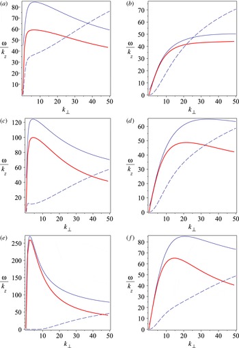
 $\text{Re}(\unicode[STIX]{x1D714})/k_{z}$
(solid line) and
 $-\text{Im}(\unicode[STIX]{x1D714})/k_{z}$
(dashed line) from kinetic theory (in dark blue) and
 $\unicode[STIX]{x1D714}/k_{z}$
from the two-field model (thick red line) for KAWs at
 $\unicode[STIX]{x1D6FD}_{e}=0.001$
(a,c,e) for
 $\unicode[STIX]{x1D70F}=1$
(a),
 $\unicode[STIX]{x1D70F}=5$
(c) and
 $\unicode[STIX]{x1D70F}=50$
(e), and at
 $\unicode[STIX]{x1D6FD}_{e}=0.1$
(b,d,f) for
 $\unicode[STIX]{x1D70F}=0.2$
(b),
 $\unicode[STIX]{x1D70F}=1$
(d) and
 $\unicode[STIX]{x1D70F}=5$
(f).

Figure 1 displays the ratios
 $\text{Re}(\unicode[STIX]{x1D714})/k_{z}$
(in dark blue solid lines) and
 $-\text{Im}(\unicode[STIX]{x1D714})/k_{z}$
(in dark blue dashed lines) obtained from the linear kinetic theory for KAWs at
 $\unicode[STIX]{x1D6FD}_{e}=0.001$
for
 $\unicode[STIX]{x1D70F}=1$
,
 $\unicode[STIX]{x1D70F}=5$
and
 $\unicode[STIX]{x1D70F}=50$
(a,c,e) and at
 $\unicode[STIX]{x1D6FD}_{e}=0.1$
for
 $\unicode[STIX]{x1D70F}=0.2$
,
 $\unicode[STIX]{x1D70F}=1$
and
 $\unicode[STIX]{x1D70F}=5$
(b,d,f). Superimposed in thick red solid lines are the corresponding ratios
 $\unicode[STIX]{x1D714}/k_{z}$
of the isothermal dispersion relation given by (6.1). At small
 $\unicode[STIX]{x1D6FD}_{e}$
, the agreement between kinetic theory and the isothermal model is better for large values of
 $\unicode[STIX]{x1D70F}$
, in part due to a smaller damping rate. A much faster decrease of the ratio
 $\text{Re}(\unicode[STIX]{x1D714})/k_{z}$
is observed for
 $\unicode[STIX]{x1D70F}=50$
and the behaviour is indeed close to that of WWs (see figure 2
b), as predicted by inspection of the dispersion relations. For smaller values of
 $\unicode[STIX]{x1D70F}$
and/or larger values of
 $\unicode[STIX]{x1D6FD}_{e}$
, the damping becomes quite strong when
 $k_{\bot }$
reaches a few units.
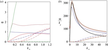
(a) Frequencies (solid) and damping rates (dashed) at
 $\unicode[STIX]{x1D6FD}_{e}=0.01$
,
 $\unicode[STIX]{x1D70F}=8$
and
 $\unicode[STIX]{x1D703}_{\boldsymbol{k}\boldsymbol{B}}=82^{\circ }$
for an Alfvén wave (red), a fast wave ending in the first Bernstein mode (blue) and in the second one (brown) and for the whistler wave (green) continuing to small scale (see right in red dotted line). (b)
 $\text{Re}(\unicode[STIX]{x1D714})/k_{z}$
(solid lines) and
 $-\text{Im}(\unicode[STIX]{x1D714})/k_{z}$
(dashed lines) from kinetic theory for whistlers at
 $\unicode[STIX]{x1D6FD}_{e}=0.01$
for
 $\unicode[STIX]{x1D70F}=0.2$
(dark blue),
 $\unicode[STIX]{x1D70F}=1$
(brown),
 $\unicode[STIX]{x1D70F}=5$
(green) and
 $\unicode[STIX]{x1D70F}=8$
(red dotted) and ratio
 $\unicode[STIX]{x1D714}/k_{z}$
from the two-field model (thick black line).

Turning to the WWs, it is of interest to first briefly discuss their properties when varying angles and
 $\unicode[STIX]{x1D6FD}_{e}$
. As mentioned previously, for small enough
 $\unicode[STIX]{x1D6FD}_{i}$
, WWs can be found as a continuation to small scales of the fast mode. At a sufficiently small angle of propagation, e.g.
 $60^{\circ }$
, they do not encounter any resonance, even at
 $\unicode[STIX]{x1D6FD}_{i}$
of order unity, but as the angle and/or
 $\unicode[STIX]{x1D6FD}_{i}$
increases, branches of Bernstein modes cross the whistler branch, that nevertheless remains continuous throughout the considered range of wavenumbers, if
 $\unicode[STIX]{x1D703}_{\boldsymbol{k}\boldsymbol{B}}$
and
 $\unicode[STIX]{x1D6FD}_{i}$
remain below certain thresholds. This is illustrated in figure 2(a), which displays the frequencies (solid) and damping rates (dashed) at
 $\unicode[STIX]{x1D6FD}_{e}=0.01$
,
 $\unicode[STIX]{x1D70F}=8$
and
 $\unicode[STIX]{x1D703}_{\boldsymbol{k}\boldsymbol{B}}=82^{\circ }$
for an Alfvén wave (red), a fast wave ending in the first Bernstein mode (blue) and in the second one (brown) and for the whistler wave (green) continuing to small scale (as a red dotted line in (b)). Choosing
 $\unicode[STIX]{x1D703}_{\boldsymbol{k}\boldsymbol{B}}=82^{\circ }$
and
 $\unicode[STIX]{x1D6FD}_{e}=0.01$
, we display in figure 2(b),
 $\text{Re}(\unicode[STIX]{x1D714})/k_{z}$
(solid lines) and
 $-\text{Im}(\unicode[STIX]{x1D714})/k_{z}$
(dashed lines) for WWs at
 $\unicode[STIX]{x1D70F}=0.2$
(dark blue),
 $\unicode[STIX]{x1D70F}=1$
(brown),
 $\unicode[STIX]{x1D70F}=5$
(green) and
 $\unicode[STIX]{x1D70F}=8$
(red dots), superimposed with the prediction of linear theory (6.2) (thick black line). As
 $\unicode[STIX]{x1D70F}$
increases, the kinetic results converge to the same curve which is very close to the prediction of the model, as long as dissipation remains small (i.e. for
 $k_{\bot }\leqslant 10$
). A very similar behaviour is observed for a
 $75^{\circ }$
propagation angle.
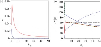
Figure 3(a) displays the electron density fluctuation of the eigenmode, obtained from the kinetic theory for KAWs (red line) at
 $\unicode[STIX]{x1D703}_{\boldsymbol{k}\boldsymbol{B}}=89.99^{\circ }$
and WWs (dark blue line) at
 $\unicode[STIX]{x1D703}_{\boldsymbol{k}\boldsymbol{B}}=82^{\circ }$
for
 $\unicode[STIX]{x1D6FD}=0.01$
and
 $\unicode[STIX]{x1D70F}=5$
. This result, which remains true at larger values of
 $\unicode[STIX]{x1D6FD}_{e}$
, confirms the assumption that was used to distinguish the two waves, namely that the WWs are associated with almost incompressible motions.
(a) Electron density fluctuations for whistlers at
 $\unicode[STIX]{x1D703}_{\boldsymbol{k}\boldsymbol{B}}=82^{\circ }$
(dark blue) and KAWs at
 $\unicode[STIX]{x1D703}_{\boldsymbol{k}\boldsymbol{B}}=89.99^{\circ }$
(red) for
 $\unicode[STIX]{x1D6FD}_{e}=0.01$
and
 $\unicode[STIX]{x1D70F}=5$
. (b)
 $\text{Re}(\unicode[STIX]{x1D714})/k_{z}$
for a KAW at
 $\unicode[STIX]{x1D6FD}_{e}=0.0001$
and
 $\unicode[STIX]{x1D70F}=1$
, from kinetic theory (in dark blue) and frequency from various two-field models: from (6.1) (thick red line), from the model of Zocco & Schekochihin (Reference Zocco and Schekochihin2011) taken in the isothermal limit (dashed black line), and from an extension of the current model using the improved relation between
 $n$
and
 $\unicode[STIX]{x1D711}$
given by (5.21) (green dotted line). The dark blue dashed line displays
 $-\text{Im}(\unicode[STIX]{x1D714})/k_{z}$
.

Finally, figure 3(b) displays the case of a smaller
 $\unicode[STIX]{x1D6FD}_{e}$
for KAWs, a situation where the behaviour at small
 $k_{\bot }$
is now quite sensitive to the ion response. We display
 $\text{Re}(\unicode[STIX]{x1D714})/k_{z}$
for
 $\unicode[STIX]{x1D6FD}_{e}=10^{-4}$
and
 $\unicode[STIX]{x1D70F}=1$
for the kinetic theory (dark blue solid line) and different models. The prediction of (6.1), which is displayed with a thick red solid line, shows a strong disagreement for
 $k_{\bot }<5$
. The agreement with kinetic theory is however much better at these large scales when using the dispersion relation of the model of Zocco & Schekochihin (Reference Zocco and Schekochihin2011) taken in the isothermal limit (black dashed line). Note that the different curvature of the dispersion relation, observed at small
 $k_{\bot }$
when
 $\unicode[STIX]{x1D6FD}_{e}$
crosses
 $m_{e}/m_{i}$
, is associated with the well-known transition from KAWs to inertial Alfvén waves. Interestingly, when modified by using the gyrokinetic Poisson equation (5.21) (green dots), our model reproduces for
 $\unicode[STIX]{x1D714}/k_{z}$
both the qualitative behaviour at large scales and the decrease at small scales, in agreement with kinetic theory, in spite of a different absolute level in a spectral range where the Landau damping is nevertheless so strong that the corresponding waves are rapidly dissipated.
6.2 Reduced Landau fluid model
We shall here restrict the discussion to the impact of Landau damping on the dispersion relation for KAWs. Equations (5.1)–(5.4) supplemented by (5.17)–(5.20), are linearized, and the dispersion relation computed using the MAPLE software. Figure 4 displays
 $\text{Re}(\unicode[STIX]{x1D714})/k_{z}$
(solid lines) and
 $-\text{Im}(\unicode[STIX]{x1D714})/k_{z}$
(dashed lines) for KAWs at
 $\unicode[STIX]{x1D70F}=1$
, in both cases
 $\unicode[STIX]{x1D6FD}_{e}=1$
(a) and
 $\unicode[STIX]{x1D6FD}_{e}=0.01$
(b), for different reduced models, with the kinetic theory prediction superimposed in dark blue. The green and thick red lines correspond to the isothermal and RLF models respectively. A clear extension of the spectral validity range is obtained when Landau damping is retained. The damping rate is however globally weaker than predicted by the kinetic theory, except at the largest scales, possibly pointing out the limitation of the closure assumption at small scales. It turns out that this discrepancy is not significantly reduced by retaining dynamical equations for the gyrotropic fluxes and closing the fluid hierarchy at the next order. The agreement is also not improved when instead of a closure assumption we use the low-frequency kinetic formulas given in appendix B of Passot & Sulem (Reference Passot and Sulem2007) and take for the plasma response functions Padé approximants of various orders. This observation raises the question whether Landau damping is the only dissipation mechanism acting at these scales.
 $\text{Re}(\unicode[STIX]{x1D714})/k_{z}$
(solid lines) and
 $-\text{Im}(\unicode[STIX]{x1D714})/k_{z}$
(dashed lines) for KAWs with propagation angle
 $\unicode[STIX]{x1D703}_{\boldsymbol{k}\boldsymbol{B}}=89.99^{\circ }$
, at
 $\unicode[STIX]{x1D70F}=1$
and
 $\unicode[STIX]{x1D6FD}_{e}=1$
(a) or
 $\unicode[STIX]{x1D6FD}_{e}=0.01$
(b) from kinetic theory (dark blue), the RLF model (thick red lines), the isothermal two-field model (green) and the RLF model with
 $\unicode[STIX]{x1D6FF}=0$
(violet).

Noticeably for
 $\unicode[STIX]{x1D6FD}_{e}=1$
, the comparison with kinetic theory for the real part is satisfactory up to
 $k=25$
(very close to the inverse electron Larmor radius). In the case where electron inertia and FLRs are not included (violet line), a regime where no saturation is expected, the disagreement starts around
 $k=10$
. This latter model, which can be viewed as an extension of the model of Boldyrev et al. (Reference Boldyrev, Horaites, Xia and Perez2013) including Landau damping, was originally derived in Tassi et al. (Reference Tassi, Sulem and Passot2016) (where the heat fluxes were estimated directly from the linear kinetic theory, instead of using the above approximate closure). For
 $\unicode[STIX]{x1D6FD}_{e}=0.01$
, globally similar graphs are obtained except that, saturation occurring at smaller wavenumbers, the domain where the kinetic theory is accurately reproduced is more limited.
7 Turbulent regimes
In this section, we concentrate on the isothermal models, considered in the spectral ranges
 ${\mathcal{D}}_{e}^{{<}}=\{1/\unicode[STIX]{x1D70C}_{s}\ll k_{\bot }\ll 1/d_{e}\}$
and
 ${\mathcal{D}}_{e}^{{>}}=\{1/d_{e}\ll k_{\bot }\ll 1/\unicode[STIX]{x1D70C}_{e}\}$
separately. While in the former domain, where
 $\unicode[STIX]{x1D6FF}^{2}k_{\bot }^{2}/\unicode[STIX]{x1D6FD}_{e}\ll 1$
, electron inertia is negligible, this effect is dominant in the latter, where
 $\unicode[STIX]{x1D6FF}^{2}k_{\bot }^{2}/\unicode[STIX]{x1D6FD}_{e}\gg 1$
. In both ranges, FLR effects are subdominant corrections that we will thus neglect. The energy becomes
 $$\begin{eqnarray}{\mathcal{E}}_{KAW}\propto \frac{1}{2}\int \left(\frac{1}{1+\unicode[STIX]{x1D70F}}\unicode[STIX]{x1D711}^{\ast 2}+\frac{2}{\unicode[STIX]{x1D6FD}_{e}}|\unicode[STIX]{x1D735}_{\bot }A_{\Vert }|^{2}+\frac{4\unicode[STIX]{x1D6FF}^{2}}{\unicode[STIX]{x1D6FD}_{e}^{2}}(\unicode[STIX]{x1D6E5}_{\bot }A_{\Vert })^{2}\right)\text{d}\boldsymbol{x},\end{eqnarray}$$
for the KAWs, and
 $$\begin{eqnarray}{\mathcal{E}}_{WW}\propto \frac{1}{2}\int \left(\unicode[STIX]{x1D711}^{\ast 2}+\frac{2\unicode[STIX]{x1D6FF}^{2}}{\unicode[STIX]{x1D6FD}_{e}}|\unicode[STIX]{x1D735}_{\bot }\unicode[STIX]{x1D711}^{\ast }|^{2}+\frac{4}{\unicode[STIX]{x1D6FD}_{e}^{2}}|\unicode[STIX]{x1D735}_{\bot }A_{\Vert }|^{2}+\frac{8\unicode[STIX]{x1D6FF}^{2}}{\unicode[STIX]{x1D6FD}_{e}^{3}}(\unicode[STIX]{x1D6E5}_{\bot }A_{\Vert })^{2}\right)\text{d}\boldsymbol{x},\end{eqnarray}$$
for the WWs. In more physically explicit terms, we can write
 $$\begin{eqnarray}{\mathcal{E}}_{KAW}\propto \frac{1}{2}\int \left(\frac{2}{\unicode[STIX]{x1D6FD}_{e}}|\boldsymbol{B}_{\bot }|^{2}+(\unicode[STIX]{x1D70F}+1)n^{2}+\unicode[STIX]{x1D6FF}^{2}u_{\Vert e}^{2}\right)\text{d}\boldsymbol{x}\end{eqnarray}$$
and
 $$\begin{eqnarray}{\mathcal{E}}_{WW}\propto \frac{1}{2}\int \left(\frac{2}{\unicode[STIX]{x1D6FD}_{e}}|\boldsymbol{B}|^{2}+\unicode[STIX]{x1D6FF}^{2}|\boldsymbol{u}_{e}|^{2}\right)\text{d}\boldsymbol{x}.\end{eqnarray}$$
Note that these energies are dominated by the transverse magnetic energy at the largest scales and by the parallel kinetic energy at the smallest ones. In a turbulent regime, the energy is expected to cascade to small transverse scales, resulting in an inertial range characterized by a scale-independent energy flux
 $\unicode[STIX]{x1D716}$
. The aim of this section is to phenomenologically evaluate the scaling properties of the transverse magnetic energy spectrum
 $E_{B_{\bot }}(k_{\bot })$
in such a cascade, in both regimes of strong and weak turbulence, assumed to exist and to result from three-wave interactions.
When assuming transverse isotropy, the energy flux
 $\unicode[STIX]{x1D716}$
can be estimated as
 $k_{\bot }$
times the one-dimensional spectral density, divided by the characteristic transfer time
 $\unicode[STIX]{x1D70F}_{tr}$
at this wavenumber. The regimes of strong and weak turbulence differ in the estimate of this time that, in both cases, can nevertheless be written
 $\unicode[STIX]{x1D70F}_{tr}=\unicode[STIX]{x1D70F}_{NL}^{2}/\unicode[STIX]{x1D70F}_{L}$
, where
 $\unicode[STIX]{x1D70F}_{NL}$
refers to the characteristic time of the nonlinear interactions at the corresponding scale, and
 $\unicode[STIX]{x1D70F}_{L}\sim 1/\unicode[STIX]{x1D714}$
to the inverse frequency of the considered wave at this scale.
In the strong turbulence regime, where a so-called critical balance holds, the rate of the nonlinear interactions at a given scale is comparable to the frequency of the linear wave at this scale (
 $\unicode[STIX]{x1D70F}_{NL}\sim \unicode[STIX]{x1D70F}_{L}$
), leading us to identify
 $\unicode[STIX]{x1D70F}_{tr}$
with
 $\unicode[STIX]{x1D70F}_{NL}$
. In this approach,
 $\unicode[STIX]{x1D70F}_{NL}$
is defined as the shortest of the characteristic times associated with the various nonlinear couplings, which turns out to be given by
 $\unicode[STIX]{x1D70F}_{NL}^{-1}\sim [\widehat{\unicode[STIX]{x1D711}}^{\ast },\cdot ]$
associated with the transverse strain. Note that the same estimate of the transfer time holds in the absence of waves. We are thus led to write
 $1/\unicode[STIX]{x1D70F}_{NL}\sim k_{\bot }^{2}\widehat{\unicode[STIX]{x1D711}}^{\ast }$
. An additional element used to relate the magnitude of the various fields is provided by the condition that the considered solution is an eigenmode of the linear problem, thus obeying equation (6.3). In both spectral ranges defined above, one can write the phase velocity in the asymptotic form
 $\unicode[STIX]{x1D714}/k_{\Vert }\sim k_{\bot }^{\unicode[STIX]{x1D6FC}}$
. In
 ${\mathcal{D}}_{e}^{{<}}$
, one thus has
 $\widehat{\unicode[STIX]{x1D711}}^{\ast }\sim (\unicode[STIX]{x1D714}/k_{\Vert })\widehat{A}_{\Vert }$
, leading to
 $\unicode[STIX]{x1D70F}_{NL}^{-1}\sim k_{\bot }^{1+\unicode[STIX]{x1D6FC}}\widehat{B}_{\bot }$
, while in
 ${\mathcal{D}}_{e}^{{>}}$
,
 $\widehat{\unicode[STIX]{x1D711}}^{\ast }\sim (\unicode[STIX]{x1D714}/k_{\Vert })k_{\bot }^{2}\widehat{A}_{\Vert }$
, leading to
 $\unicode[STIX]{x1D70F}_{NL}^{-1}\sim k_{\bot }^{3+\unicode[STIX]{x1D6FC}}\widehat{B}_{\bot }$
.
In the strong turbulent regime, it follows that in
 ${\mathcal{D}}_{e}^{{<}}$
, where
 $\unicode[STIX]{x1D716}\sim k_{\bot }^{1+\unicode[STIX]{x1D6FC}}\widehat{B}_{\bot }^{3}$
, one gets
 $E_{B_{\bot }}(k)\sim \unicode[STIX]{x1D716}^{2/3}k_{\bot }^{-(5+2\unicode[STIX]{x1D6FC})/3}$
, while in
 ${\mathcal{D}}_{e}^{{>}}$
, where
 $\unicode[STIX]{x1D716}\sim k_{\bot }^{5+\unicode[STIX]{x1D6FC}}\widehat{B}_{\bot }^{3}$
, one has
 $E_{B_{\bot }}(k)\sim \unicode[STIX]{x1D716}^{2/3}k_{\bot }^{-(13+2\unicode[STIX]{x1D6FC})/3}$
.
In the weak turbulent regime, one easily obtains that in
 ${\mathcal{D}}_{e}^{{<}}$
,
 $\unicode[STIX]{x1D70F}_{tr}^{-1}\sim k_{\bot }^{(2+\unicode[STIX]{x1D6FC})}B_{\bot }^{2}$
, while in
 ${\mathcal{D}}_{e}^{{>}}$
,
 $\unicode[STIX]{x1D70F}_{tr}^{-1}\sim k_{\bot }^{(6+\unicode[STIX]{x1D6FC})}B_{\bot }^{2}$
. It follows that in
 ${\mathcal{D}}_{e}^{{<}}$
,
 $E_{B_{\bot }}(k)\sim \unicode[STIX]{x1D716}^{1/2}k_{\bot }^{-(2+\unicode[STIX]{x1D6FC}/2)}$
, while in
 ${\mathcal{D}}_{e}^{{>}}$
,
 $E_{B_{\bot }}(k)\sim \unicode[STIX]{x1D716}^{1/2}k_{\bot }^{-(5+\unicode[STIX]{x1D6FC}/2)}$
. Let us now consider more specifically the cases of KAWs and WWs.
In
 ${\mathcal{D}}_{e}^{{<}}$
, the dispersion relation is the same for KAWs and WWs, with
 $\unicode[STIX]{x1D6FC}=1$
. As a consequence, for both types of waves,
 $E_{B_{\bot }}(k_{\bot })\sim \unicode[STIX]{x1D716}^{2/3}k_{\bot }^{-7/3}$
in the strong turbulent regime and
 $E_{B_{\bot }}(k_{\bot })\sim \unicode[STIX]{x1D716}^{1/2}k_{\bot }^{-5/2}$
in the weak turbulent regime, a result obtained as the finite flux solution of the weak turbulence spectral equations in Galtier & Bhattacharjee (Reference Galtier and Bhattacharjee2003).
In
 ${\mathcal{D}}_{e}^{{>}}$
, various cases are to be distinguished. For the KAWs, when the ion-to-electron temperature ratio
 $\unicode[STIX]{x1D70F}$
is moderate,
 $\unicode[STIX]{x1D6FC}=0$
. One thus obtains
 $E_{B_{\bot }}(k_{\bot })\sim \unicode[STIX]{x1D716}^{2/3}k_{\bot }^{-13/3}$
in the strong turbulent regime and
 $E_{B_{\bot }}(k_{\bot })\sim \unicode[STIX]{x1D716}^{1/2}k_{\bot }^{-5}$
in the weak turbulent regime. Note that a
 $-13/3$
exponent for the magnetic field spectra has also been reported in the different context of a generalized helicity cascade in incompressible so-called extended MHD (Krishan & Mahajan Reference Krishan and Mahajan2004; Abdelhamid, Lingam & Mahajan Reference Abdelhamid, Lingam and Mahajan2016). In contrast, for the WWs, but also for the KAWs when the ion-to–electron temperature ratio is large (
 $\unicode[STIX]{x1D70F}\gg 1$
),
 $\unicode[STIX]{x1D6FC}=-1$
. It follows that in this case
 $E_{B_{\bot }}(k_{\bot })\sim \unicode[STIX]{x1D716}^{2/3}k_{\bot }^{-11/3}$
in the strong turbulence regime and
 $E_{B_{\bot }}(k_{\bot })\sim \unicode[STIX]{x1D716}^{1/2}k_{\bot }^{-9/2}$
in the weak turbulence regime. A similar
 $k_{\bot }^{-11/3}$
spectrum for KAWs at large
 $\unicode[STIX]{x1D70F}$
is also obtained by Chen & Boldyrev (Reference Chen and Boldyrev2017).
Furthermore, in the case of strong turbulence, the spectral anisotropy can be estimated from the above relations. While at large scale, the balance between the linear term
 $\unicode[STIX]{x2202}_{z}\unicode[STIX]{x1D711}^{\ast }$
in (5.9) with the bracket
 $[\unicode[STIX]{x1D711}^{\ast },A_{\Vert }]$
leads to
 $k_{\Vert }\sim k_{\bot }^{2}\widehat{A}_{\Vert }$
and thus to the usual scaling
 $k_{\Vert }\sim k_{\bot }^{1/3}$
, at small scales the relevant nonlinear term is
 $[\unicode[STIX]{x1D711}^{\ast },(2\unicode[STIX]{x1D6FF}^{2}/\unicode[STIX]{x1D6FD}_{e})\unicode[STIX]{x1D6E5}_{\bot }A_{\Vert }]$
. In this regime,
 $k_{\Vert }\sim k_{\bot }^{4}\widehat{A}_{\Vert }$
where
 $\widehat{A}_{\Vert }\sim k_{\bot }^{-8/3-\unicode[STIX]{x1D6FC}/3}$
. For KAWs with
 $\unicode[STIX]{x1D70F}\sim 1$
,
 $\unicode[STIX]{x1D6FC}=0$
, this implies
 $k_{\Vert }\sim k_{\bot }^{4/3}$
, while for WWs or KAWs at
 $\unicode[STIX]{x1D70F}\gg 1$
, one has
 $k_{\Vert }\sim k_{\bot }^{5/3}$
, consistent with the finding of Chen & Boldyrev (Reference Chen and Boldyrev2017). In both cases, the longitudinal transfer becomes increasingly important at smaller scales.
It is also of interest to consider the effect of a small but finite value of
 $\unicode[STIX]{x1D6FD}_{e}$
on the energy spectrum. Considering the case of KAWs, figure 3(b) shows that taking
 $\unicode[STIX]{x1D6FD}_{e}=10^{-4}$
causes
 $\unicode[STIX]{x1D714}/k_{\Vert }$
to decrease with
 $k_{\bot }$
(red solid and green dotted lines), while it tends to a constant when
 $\unicode[STIX]{x1D6FD}_{e}=0$
(black dashed line). As the spectrum can be written in the form
 $k_{\bot }^{-13/3}(\unicode[STIX]{x1D714}/k_{\Vert })^{-2/3}$
, this suggests that a finite
 $\unicode[STIX]{x1D6FD}_{e}$
will tend to make the spectrum shallower.
At the numerical level, simulations of whistler turbulence were performed using incompressible bi-fluid equations in 2.5-D (i.e. three-dimensional velocities and magnetic fields but two-dimensional space coordinates), showing a transition from a
 $-7/3$
spectrum at the ion scales to a steeper slope (close to
 $-11/3$
) at scales smaller than
 $d_{e}$
(Andrés et al.
Reference Andrés, Gonzalez, Martin, Dmitruk and Gómez2014). Three-dimensional particle-in-cell simulations of WW turbulence also clearly indicate the development of two sub-ion spectral ranges, but the exponents are steeper than those predicted by the above phenomenology, and non-universal (Chang, Gary & Wang Reference Chang, Gary and Wang2011; Gary et al.
Reference Gary, Chang and Wang2012). Kinetic effects, such as electron Landau damping could be at the origin of this discrepancy. This issue could be addressed with the RLF model (discussed in § 5.3), both numerically and using a phenomenological approach as in Passot & Sulem (Reference Passot and Sulem2015). Concerning the kinetic Alfvén wave cascade, the phenomenology discussed above assumes a transformation of Alfvén waves to KAWs near the ion gyroscale. Recent numerical simulations (Cerri & Califano Reference Cerri and Califano2017) however indicate that fast magnetic reconnection processes can inject energy on a time scale shorter than the nonlinear cascade time at the reconnection scales, leading to the formation of
 $d_{i}$
-scale structures and to a nonlinear cascade that fills the spectrum at small scales. The effect of such phenomena on the sub-ion turbulence remains to be analysed quantitatively, possibly using reduced fluid models.
8 Conclusion
Reduced fluid models have been derived for the sub-ion-scale dynamics of collisionless plasmas, retaining electron inertia and leading-order electron FLR corrections. Neglecting the ion dynamics, we are led to discriminate between two limiting cases: a low-frequency regime involving perpendicular pressure balance and a high-frequency one, where the electron fluid is essentially incompressible. The two resulting models capture KAWs and WWs respectively, in the context of isothermal or Landau fluid closures. They extend the validity range of previously existing models. At small
 $\unicode[STIX]{x1D6FD}_{e}$
and scales large compared to
 $d_{e}$
, they both reduce to ERMHD (Schekochihin et al.
Reference Schekochihin, Cowley, Dorland, Hammett, Howes, Quataert and Tatsuno2009; Boldyrev et al.
Reference Boldyrev, Horaites, Xia and Perez2013) where the same equations govern different fields depending on the kind of waves. Furthermore, at scales comparable to
 $d_{e}$
, in 2.5-D dimensions and for
 $\unicode[STIX]{x1D6FD}_{e}$
small enough for electron FLR corrections to be negligible (i.e.
 $\unicode[STIX]{x1D6FD}_{e}=O(m_{e}/m_{i})$
), the system for WWs reproduces EMHD (see e.g. (10)–(11) of Biskamp et al.
Reference Biskamp, Schwarz, Zeiler, Celani and Drake1999). Differently, in the same
 $\unicode[STIX]{x1D6FD}_{e}$
-range, the equations for KAWs with the Landau fluid closure appear as a fluid reduction of those of Zocco & Schekochihin (Reference Zocco and Schekochihin2011) (see Loureiro, Schekochihin & Zocco (Reference Loureiro, Schekochihin and Zocco2013) for their numerical simulations in the case of fast collisionless reconnection). While the latter model is based on a drift kinetic description of the electrons, the present RLF model includes first-order FLR corrections. Such terms, together with the contribution of parallel magnetic fluctuations, which are both
 $O(\unicode[STIX]{x1D6FD}_{e})$
, induce a sensitivity of the system to pressure anisotropy, an effect potentially important in a reconnection context (Lee et al.
Reference Lee, Daughton, Karimabadi and Egedal2016).
Computation of the electron gyroviscous force
 $\unicode[STIX]{x1D735}\boldsymbol{\cdot }\unicode[STIX]{x1D72B}_{e}$
is performed within an asymptotic expansion based on temporal and spatial scale separation between the electron gyroradius and the considered quasi-transverse scales, a procedure which, at scales comparable to
 $d_{e}$
, results in an expansion in terms of
 $\unicode[STIX]{x1D6FD}_{e}$
. The computation involves a recursive process involving both the non-gyrotropic pressure and heat flux tensors, two iterations being needed in order to obtain the leading order in
 $\unicode[STIX]{x1D6FD}_{e}$
. Because of the algebraic complexity in the general framework (see e.g. Ramos Reference Ramos2005a
), we resorted in the present paper to assume a gyrotropic heat flux in the expression of the gyroviscous force. Relations with previous FLR estimates is discussed in appendix B. Note that including the gyroviscous force in a generalized Ohm’s law may in particular be useful for enriching hybrid models in the context of collisionless reconnection.
Both isothermal and Landau fluid closures are considered for KAWs and WWs. The linear regime is examined in comparison with the fully kinetic theory to evaluate the validity of these closures. In the isothermal case, a qualitative agreement is found, which turns out to be more accurate when Landau damping is weak. For the propagation angles exceeding
 $80^{\circ }$
that we have considered, WWs are more weakly damped than KAWs, at least at scales larger than
 $\unicode[STIX]{x1D70C}_{e}$
. As expected, for the values of
 $\unicode[STIX]{x1D6FD}_{e}\lesssim 0.1$
and moderate values of
 $\unicode[STIX]{x1D70F}$
, the range of angles where KAWs can propagate without resonance turns out to be restricted to quasi-perpendicular angles. The Landau fluid closure improves the model accuracy. In particular, when
 $\unicode[STIX]{x1D6FD}_{e}$
is pushed to values of order unity, the range of wavenumbers where the dispersion relation is accurately described is significantly enlarged.
Observations in the solar wind and the magnetosheath provide evidence of power-law magnetic energy spectra at scales smaller than
 $d_{e}$
, possibly associated with turbulent cascades. Assuming that KAWs and WWs are still present at such scales, we explored the spectrum of the transverse magnetic fluctuations in both strong and weak turbulence energy cascades. As a first step, a phenomenological approach where FLR corrections are neglected is presented. In addition to the well-known WWs magnetic spectra both above and below
 $d_{e}^{-1}$
, and to the
 $-7/3$
sub-ion KAWs spectrum, a new regime of KAW turbulence is obtained at scales smaller than
 $d_{e}$
, characterized by a
 $-13/3$
exponent for strong turbulence and by a
 $-5$
exponent in the weak regime. These exponents are to be compared with satellite observational data that display slopes steeper than the WWs
 $-11/3$
spectrum. Note that other physical effects such as Landau damping (Passot & Sulem Reference Passot and Sulem2015; Sulem et al.
Reference Sulem, Passot, Laveder and Borgogno2016) and intermittency corrections associated with coherent structures, such as current sheets (Boldyrev et al.
Reference Boldyrev, Horaites, Xia and Perez2013), can also lead to steeper spectra. It should be stressed that both phenomenological arguments and numerical simulations predict a transition at
 $d_{e}$
, while observational spectra in the terrestrial magnetosheath only display a transition at
 $\unicode[STIX]{x1D70C}_{e}$
(Huang et al.
Reference Huang, Sahraoui, Deng, He, Yuan, Zhou, Pang and Fu2014), associated with electron demagnetization. In fact, a transition at
 $d_{e}$
is more clearly observed at the level of the magnetic compressibility (Chen & Boldyrev Reference Chen and Boldyrev2017). This does exclude that additional effects such as other kind of waves or structures could play a role.
As shown in § 5, our four-field model, as well as its two-field isothermal reductions, conserve energy. To the best of our knowledge, this is the first example of reduced fluid model for inertial reconnection conserving energy and accounting for electron FLR effects. A question we intend to address in the future concerns the Hamiltonian structure of this model. Previous results concerning the inclusion of (ion) FLR effects in Hamiltonian reduced fluid models were presented in Morrison, Caldas & Tasso (Reference Morrison, Caldas and Tasso1984), Hazeltine, Hsu & Morrison (Reference Hazeltine, Hsu and Morrison1987), Dagnelund & Pavlenko (Reference Dagnelund and Pavlenko2005), Izacard et al. (Reference Izacard, Chandre, Tassi and Ciraolo2011), Morrison, Lingam & Acevedo (Reference Morrison, Lingam and Acevedo2014). It could in particular be of interest to investigate whether the idea of the gyromap transformation, adopted in Morrison et al. (Reference Morrison, Caldas and Tasso1984), Hazeltine et al. (Reference Hazeltine, Hsu and Morrison1987), Izacard et al. (Reference Izacard, Chandre, Tassi and Ciraolo2011), Morrison et al. (Reference Morrison, Lingam and Acevedo2014) together with the Hamiltonian structure of the model in the absence of FLR contributions, can help in building a Hamiltonian model including electron FLR effects. Further developments should also include numerical simulations to test the predictions for the turbulent energy spectra, and in particular to evaluate the role of coherent structures and analyse the difference between two- and three-dimensional geometries. Existence and stability of Alfvén or electron vortices (Mikhalovskii et al.
Reference Mikhalovskii, Lakhin, Aburdzhaniya, Mikhailovskaya, Onishchenko and Smolyakov1987; Schep, Pegoraro & Kuvshinov Reference Schep, Pegoraro and Kuvshinov1994) are also open questions. Other open issues concern the relative importance of KAWs and WWs in space plasmas. Such questions cannot be addressed using gyrokinetic simulations or gyrofluid models which, involving a perpendicular pressure balance, concentrate on low-frequency waves. Furthermore, the models for the WWs and the KAWs considered in this paper differentiate at the level of the determination of the magnitude of the density fluctuations. When the latter are neglected, the system can be viewed as an extension of EMHD for WWs to smaller scales, while when pressure balance is prescribed, it describes KAWs dynamics. It would be of great interest to derive a reduced fluid model able to simultaneously capture the two types of wave. Noticibly, recent hybrid kinetic simulations indicate that the relative importance of KAWs and WWs is sensitive to the plasma
 $\unicode[STIX]{x1D6FD}$
, KAWs being dominant at
 $\unicode[STIX]{x1D6FD}\gtrsim 1$
and WWs at lower
 $\unicode[STIX]{x1D6FD}$
(Cerri et al.
Reference Cerri, Califano, Jenko, Told and Rincon2016).
In addition to turbulent cascades discussed in this paper, an important issue that the present models can address concerns collisionless magnetic reconnection, in particular in three dimensions where fully kinetic simulations require huge computational resources. In the turbulent regime, RLF models could in particular provide an efficient tool to study the relative contributions of coherent structure disruptions and incoherent fluctuation cascades in the processes of dissipation and plasma heating (Parashar et al. Reference Parashar, Salem, Wicks, Karimabadi, Gary and Matthaeus2015), an important issue aimed at being addressed by the THOR satellite mission (Vaivads et al. Reference Vaivads, Retinò, Soucek, Khotyaintsev, Valentini, Escoubet, Alexandrova, André, Bale and Balikhin2016).
Appendix A. Nongyrotropic electron pressure tensor
As derived in Schekochihin et al. (Reference Schekochihin, Cowley, Rincon and Rosin2010), an exact equation for the electron pressure tensor
 $\unicode[STIX]{x1D64B}_{e}$
reads, when neglecting collisions,
 $$\begin{eqnarray}\displaystyle \unicode[STIX]{x1D617}_{e,ij} & = & \displaystyle p_{\bot e}\unicode[STIX]{x1D6FF}_{ij}+(p_{\bot e}-p_{\Vert e})\widehat{b}_{i}\widehat{b}_{j}\nonumber\\ \displaystyle & & \displaystyle +\,\unicode[STIX]{x1D6FF}^{2}\frac{\unicode[STIX]{x1D614}_{ijkl}}{4B}\left[\frac{\text{D}^{(e)}}{\text{D}t}\unicode[STIX]{x1D617}_{e,kl}+\unicode[STIX]{x2202}_{m}\unicode[STIX]{x1D618}_{e,mkl}+(\unicode[STIX]{x1D6FF}_{mn}\unicode[STIX]{x1D617}_{e,kl}+\unicode[STIX]{x1D6FF}_{kn}\unicode[STIX]{x1D617}_{e,ml}+\unicode[STIX]{x1D6FF}_{ln}\unicode[STIX]{x1D617}_{e,mk})\unicode[STIX]{x2202}_{m}u_{e,n}\right]\!.\qquad\end{eqnarray}$$
In this equation,
 $\unicode[STIX]{x1D64C}_{e}$
denotes the heat flux tensor and
 $$\begin{eqnarray}\unicode[STIX]{x1D614}_{ijkl}=(\unicode[STIX]{x1D6FF}_{ik}+3\widehat{b}_{i}\widehat{b}_{k})\unicode[STIX]{x1D716}_{jln}\widehat{b}_{n}+\unicode[STIX]{x1D716}_{iln}\widehat{b}_{n}(\unicode[STIX]{x1D6FF}_{jk}+3\widehat{b}_{j}\widehat{b}_{k}).\end{eqnarray}$$
Equation (A 1) can be solved recursively, using as small parameters
 $\unicode[STIX]{x1D6FF}^{2}\unicode[STIX]{x1D714}$
and
 $\unicode[STIX]{x1D6FF}^{2}k^{2}$
, corresponding in the dimensional variables to the conditions that the considered scales
 $k^{-1}$
be large and the frequencies
 $\unicode[STIX]{x1D714}$
small compared to the electron Larmor radius and cyclotron frequency respectively. For
 $\unicode[STIX]{x1D6FD}_{e}$
of order unity, this also prescribes that scales must be large compared to
 $d_{e}$
. In this regime, the appropriate scaling is that given by (3.13) of Tassi et al. (Reference Tassi, Sulem and Passot2016). Differently, for small values of
 $\unicode[STIX]{x1D6FD}_{e}$
, scales comparable to
 $d_{e}$
can be considered, the appropriate scaling being that given in § 2. Keeping the leading-order corrections in
 $\unicode[STIX]{x1D6FD}_{e}$
nevertheless requires in this case to also retain the second order relatively to the scale expansion, as shown below. In the following, we shall concentrate on the small
 $\unicode[STIX]{x1D6FD}_{e}$
regime, but the resulting gyroviscous force remains valid at
 $\unicode[STIX]{x1D6FD}_{e}=O(1)$
(recalling that, in the present units,
 $k$
must remain small compared to
 $(m_{i}/2m_{e})^{1/2}\approx 30$
), although it then includes subdominant contributions.
The iteration mentioned above involves in fact the coupling with another equation for the heat flux tensor (not written here). Solving the coupled system proves to be quite involved and falls outside the scope of the present paper. A linear version can be found in Goswami et al. (Reference Goswami, Passot and Sulem2005). Here, for the sake of simplicity, we resorted to only retain the contribution of the gyrotropic part of
 $\unicode[STIX]{x1D64C}_{e}$
in the evaluation of the gyroviscous stress.
A.1 First-order contributions
At zeroth order, the pressure tensor is simply given by its gyrotropic expression
 $\unicode[STIX]{x1D64B}_{e}^{G}=p_{\bot e}\unicode[STIX]{x1D644}+(p_{\bot e}-p_{\Vert e})\unicode[STIX]{x1D749}$
. At first order, replacing
 $\unicode[STIX]{x1D64B}_{e}$
by
 $\unicode[STIX]{x1D64B}_{e}^{G}$
in the right-hand side of (A 1), we easily get for the gyroviscous tensor
 $$\begin{eqnarray}\unicode[STIX]{x1D72B}_{e}^{(1)}=-\frac{\unicode[STIX]{x1D6FF}^{2}}{4B}[\widehat{\boldsymbol{b}}\times \unicode[STIX]{x1D652}\boldsymbol{\cdot }(\unicode[STIX]{x1D644}+3\,\unicode[STIX]{x1D749})-(\unicode[STIX]{x1D644}+3\,\unicode[STIX]{x1D749})\boldsymbol{\cdot }\unicode[STIX]{x1D652}\times \widehat{\boldsymbol{b}}]-\frac{\unicode[STIX]{x1D6FF}^{2}}{B}[\widehat{\boldsymbol{b}}\otimes (\boldsymbol{w}\times \widehat{\boldsymbol{b}})+(\boldsymbol{w}\times \widehat{\boldsymbol{b}})\otimes \widehat{\boldsymbol{b}}].\end{eqnarray}$$
Here,
 $$\begin{eqnarray}\unicode[STIX]{x1D652}=[p_{\bot e}\unicode[STIX]{x1D735}\boldsymbol{u}_{e}+\unicode[STIX]{x1D735}(q_{\bot e}\,\widehat{\boldsymbol{b}})]^{S}\end{eqnarray}$$
and
 $$\begin{eqnarray}\boldsymbol{w}=(p_{\bot e}-p_{\Vert e})\left(\frac{\text{d}\widehat{\boldsymbol{b}}}{\text{d}t}+\unicode[STIX]{x1D6FB}_{\Vert }\boldsymbol{u}_{e}\right)+(3q_{\bot e}-q_{\Vert e})\unicode[STIX]{x1D6FB}_{\Vert }\widehat{\boldsymbol{b}},\end{eqnarray}$$
where, for a given tensor
 $\unicode[STIX]{x1D64F}$
, the notation
 $\unicode[STIX]{x1D64F}^{S}$
denotes the sum of the tensor with the ones obtained by circular permutation of the indices. Assuming an equilibrium state with isotropic temperatures, the term
 $w$
is of order
 $O(\unicode[STIX]{x1D700}^{3})$
in the present asymptotics and can thus be neglected. We thus write
 $\unicode[STIX]{x1D72B}_{e}^{(1)}=\unicode[STIX]{x1D72B}_{e}^{(1,u)}+\unicode[STIX]{x1D72B}_{e}^{(1,q)}$
where
 $$\begin{eqnarray}\unicode[STIX]{x1D72B}_{e}^{(1,u)}=-\frac{\unicode[STIX]{x1D6FF}^{2}}{4B}[\widehat{\boldsymbol{b}}\times [p_{\bot e}\unicode[STIX]{x1D735}\boldsymbol{u}_{e}]^{S}\boldsymbol{\cdot }(\unicode[STIX]{x1D644}+3\,\unicode[STIX]{x1D749})-(\unicode[STIX]{x1D644}+3\,\unicode[STIX]{x1D749})\boldsymbol{\cdot }[p_{\bot e}\unicode[STIX]{x1D735}\boldsymbol{u}_{e}]^{S}\times \widehat{\boldsymbol{b}}],\end{eqnarray}$$
and where
 $\unicode[STIX]{x1D72B}_{e}^{(1,q)}$
and all the quantities derived from it can be obtained from the formula involving
 $\unicode[STIX]{x1D72B}_{e}^{(1,u)}$
after the replacements
 $p_{\bot e}$
by 1 and
 $\boldsymbol{u}_{e}$
by
 $q_{\bot e}\widehat{\boldsymbol{b}}$
. Equation (A 6) identifies with (C 1) of Ramos (Reference Ramos2005b
), up to the minus sign due to the electron charge.
A.1.1 Velocity contributions
Carrying out calculations similar to those performed in Ramos (Reference Ramos2005b ), we obtain, without neglecting any possibly subdominant contribution,
 $$\begin{eqnarray}\displaystyle \unicode[STIX]{x1D735}\boldsymbol{\cdot }\unicode[STIX]{x1D72B}_{e}^{(1,u)} & = & \displaystyle \overbrace{-\unicode[STIX]{x1D6FF}^{2}\left[\unicode[STIX]{x1D735}\times \left(\frac{p_{\bot e}}{B}\widehat{\boldsymbol{b}}\right)\boldsymbol{\cdot }\unicode[STIX]{x1D735}\right]\boldsymbol{u}_{e}}^{\unicode[STIX]{x2460}}+\overbrace{\frac{\unicode[STIX]{x1D6FF}^{2}}{2}\unicode[STIX]{x1D735}\left(\frac{p_{\bot e}\unicode[STIX]{x1D714}_{\Vert e}}{B}\right)}^{\unicode[STIX]{x2461}}\nonumber\\ \displaystyle & & \displaystyle \overbrace{+\,\unicode[STIX]{x1D6FF}^{2}\unicode[STIX]{x1D735}\times \left(\frac{p_{\bot e}}{B}\unicode[STIX]{x1D6FB}_{\Vert }\boldsymbol{u}_{e}\right)}^{\unicode[STIX]{x2462}}\overbrace{+\,\frac{\unicode[STIX]{x1D6FF}^{2}}{2}\unicode[STIX]{x1D735}\times ((\unicode[STIX]{x1D735}\boldsymbol{\cdot }\boldsymbol{u}_{e})\widehat{\boldsymbol{b}})}^{\unicode[STIX]{x2463}}\overbrace{-\,\frac{3\unicode[STIX]{x1D6FF}^{2}}{2}\unicode[STIX]{x1D735}\times (\widehat{\boldsymbol{b}}\boldsymbol{\cdot }(\unicode[STIX]{x1D6FB}_{\Vert }\boldsymbol{u}_{e})\widehat{\boldsymbol{b}})}^{\unicode[STIX]{x2464}}\nonumber\\ \displaystyle & & \displaystyle \overbrace{-\,3\unicode[STIX]{x1D6FF}^{2}B\unicode[STIX]{x1D6FB}_{\Vert }\left(\frac{p_{\bot e}}{B^{2}}\widehat{\boldsymbol{b}}\times \unicode[STIX]{x1D6FB}_{\Vert }\boldsymbol{u}_{e}\right)}^{\unicode[STIX]{x2465}}\overbrace{-\,\frac{3\unicode[STIX]{x1D6FF}^{2}}{2}B\unicode[STIX]{x1D6FB}_{\Vert }\left(\frac{p_{\bot e}}{B^{2}}\unicode[STIX]{x1D714}_{\Vert e}\widehat{\boldsymbol{b}}\right)}^{\unicode[STIX]{x2466}}\overbrace{+\,\unicode[STIX]{x1D6FF}^{2}B\unicode[STIX]{x1D6FB}_{\Vert }\left(\frac{p_{\bot e}}{B^{2}}\unicode[STIX]{x1D74E}_{e}\right)}^{\unicode[STIX]{x2467}},\qquad\end{eqnarray}$$
where
 $\unicode[STIX]{x1D74E}_{e}=\unicode[STIX]{x1D735}\times \boldsymbol{u}_{e}$
.
Let us first calculate
 $\widehat{\boldsymbol{b}}\boldsymbol{\cdot }\unicode[STIX]{x1D735}\boldsymbol{\cdot }\unicode[STIX]{x1D72B}_{e}^{(1,u)}$
, which enters (2.18) where all the terms scale as
 $\unicode[STIX]{x1D6FF}\unicode[STIX]{x1D700}^{2}$
for the KAWs or
 $\unicode[STIX]{x1D6FD}_{e}^{1/2}\unicode[STIX]{x1D6FF}\unicode[STIX]{x1D700}^{2}$
for the WWs (when the scaling parameter
 $\unicode[STIX]{x1D707}$
is replaced by
 $\unicode[STIX]{x1D6FF}/\unicode[STIX]{x1D6FD}_{e}^{1/2}$
). Thus, in (A 7), only contributions of these orders, possibly up to factors of order
 $O(\unicode[STIX]{x1D6FD}_{e})$
(which is assumed to be only ‘moderately’ small) are to be kept. It follows that the contributions of the terms
 $\unicode[STIX]{x2463}$
–
 $\unicode[STIX]{x2465}$
, which scale like
 $\unicode[STIX]{x1D700}^{3}$
(since in particular
 $\unicode[STIX]{x1D735}\boldsymbol{\cdot }\boldsymbol{u}_{e}$
is of second order in
 $\unicode[STIX]{x1D700}$
for the KAWs and even smaller for the WWs), are negligible. The relevant contributions are: from term
 $\unicode[STIX]{x2460}$
,
 $\unicode[STIX]{x1D6FF}^{2}[p_{\bot e}-B_{z},u_{\Vert e}]$
; from term
 $\unicode[STIX]{x2461}$
,
 $(\unicode[STIX]{x1D6FF}^{2}/2)\unicode[STIX]{x1D6FB}_{\Vert }\unicode[STIX]{x1D714}_{ze}$
; from term
 $\unicode[STIX]{x2462}$
,
 $\unicode[STIX]{x1D6FF}^{2}\widehat{\boldsymbol{z}}\boldsymbol{\cdot }\unicode[STIX]{x1D735}\times \unicode[STIX]{x1D6FB}_{\Vert }\boldsymbol{u}_{\bot e}$
; from term
 $\unicode[STIX]{x2466}$
,
 $-(3\unicode[STIX]{x1D6FF}^{2}/2)\unicode[STIX]{x1D6FB}_{\Vert }\unicode[STIX]{x1D714}_{ze}$
; from term
 $\unicode[STIX]{x2467}$
,
 $\unicode[STIX]{x1D6FF}^{2}\unicode[STIX]{x1D6FB}_{\Vert }\unicode[STIX]{x1D714}_{ze}$
. We thus obtain
 $$\begin{eqnarray}\widehat{\boldsymbol{b}}\boldsymbol{\cdot }\unicode[STIX]{x1D735}\boldsymbol{\cdot }\unicode[STIX]{x1D72B}_{e}^{(1,u)}=\unicode[STIX]{x1D6FF}^{2}\{[p_{\bot e}-B_{z},u_{\Vert e}]+\widehat{\boldsymbol{z}}\boldsymbol{\cdot }\unicode[STIX]{x1D735}\times \unicode[STIX]{x1D6FB}_{\Vert }\boldsymbol{u}_{\bot e}\}.\end{eqnarray}$$
Note that, in terms of
 $\unicode[STIX]{x1D711}^{\ast }$
, we can write
 $$\begin{eqnarray}\widehat{\boldsymbol{z}}\boldsymbol{\cdot }\unicode[STIX]{x1D735}\times \unicode[STIX]{x1D6FB}_{\Vert }\boldsymbol{u}_{\bot e}=\unicode[STIX]{x1D6FB}_{\Vert }\unicode[STIX]{x1D6E5}_{\bot }\unicode[STIX]{x1D711}^{\ast }+\mathop{\sum }_{i=x,y}[\unicode[STIX]{x2202}_{i}\unicode[STIX]{x1D711}^{\ast },\unicode[STIX]{x2202}_{i}A_{\Vert }].\end{eqnarray}$$
Furthermore, the term
 $\unicode[STIX]{x1D6FF}^{2}[p_{\bot e}-B_{z},u_{\Vert e}]$
, which participates to the so-called gyroviscous cancellation, is
 $O(\unicode[STIX]{x1D6FF}\unicode[STIX]{x1D700}^{2})$
for the KAWs, thus larger than all the other contributions, which are
 $O(\unicode[STIX]{x1D6FD}_{e}\unicode[STIX]{x1D6FF}\unicode[STIX]{x1D700}^{2})$
. Differently, for the WWs, all the terms are
 $O(\unicode[STIX]{x1D6FD}^{3/2}\unicode[STIX]{x1D6FF}\unicode[STIX]{x1D700}^{2})$
.
It is also easy to obtain the transverse component of
 $\unicode[STIX]{x1D735}\boldsymbol{\cdot }\unicode[STIX]{x1D72B}_{e}^{(1,u)}$
, which reads
 $$\begin{eqnarray}\displaystyle (\unicode[STIX]{x1D735}\boldsymbol{\cdot }\unicode[STIX]{x1D72B}_{e}^{(1,u)})_{\bot } & = & \displaystyle \unicode[STIX]{x1D6FF}^{2}\left\{[p_{\bot e}-B_{z},\boldsymbol{u}_{\bot e}]+\frac{1}{2}\unicode[STIX]{x1D735}_{\bot }\left(\frac{p_{\bot e}}{B}\unicode[STIX]{x1D714}_{\Vert e}\right)\right.\nonumber\\ \displaystyle & & \displaystyle +\left.\frac{1}{2}\unicode[STIX]{x1D735}_{\bot }\times [(\unicode[STIX]{x1D735}\boldsymbol{\cdot }\boldsymbol{u}_{e}-\unicode[STIX]{x1D6FB}_{\Vert }u_{\Vert e})\widehat{\boldsymbol{z}}]+\unicode[STIX]{x1D6FB}_{\Vert }\unicode[STIX]{x1D735}\times (u_{\Vert e}\widehat{\boldsymbol{z}})\vphantom{\left(\frac{p_{\bot e}}{B}\unicode[STIX]{x1D714}_{\Vert e}\right)}\right\},\end{eqnarray}$$
where an expression involving a bracket with a scalar as one argument and a vector as the other one stands for the vector whose components are obtained as the brackets of the scalar with each components of the vector.
The dominant contribution to
 $(\unicode[STIX]{x1D735}\boldsymbol{\cdot }\unicode[STIX]{x1D72B}_{e}^{(1,u)})_{\bot }$
, which enters (2.9), originates from the second term on the right-hand side and writes
 $(\unicode[STIX]{x1D6FF}^{2}/2)\unicode[STIX]{x1D735}\unicode[STIX]{x1D714}_{ze}$
. It is
 $O(\unicode[STIX]{x1D6FD}_{e}\unicode[STIX]{x1D700})$
for both types of wave. For the KAWs, the other terms are
 $O(\unicode[STIX]{x1D6FD}_{e}^{1/2}\unicode[STIX]{x1D6FF}\unicode[STIX]{x1D700}^{2})$
, or
 $O(\unicode[STIX]{x1D6FD}_{e}^{3/2}\unicode[STIX]{x1D6FF}\unicode[STIX]{x1D700}^{2})$
for the term involving
 $B_{z}$
, while for the WWs, they are all
 $O(\unicode[STIX]{x1D6FD}^{3/2}\unicode[STIX]{x1D6FF}\unicode[STIX]{x1D700}^{2})$
.
A.1.2 Heat flux contributions
Let us now consider the contributions involving
 $\unicode[STIX]{x1D72B}_{e}^{(1,q)}$
. It is easy to find that
 $$\begin{eqnarray}\widehat{\boldsymbol{b}}\boldsymbol{\cdot }\unicode[STIX]{x1D735}\boldsymbol{\cdot }\unicode[STIX]{x1D72B}_{e}^{(1,q)}=-\unicode[STIX]{x1D6FF}^{2}[B_{z},q_{\bot e}]\end{eqnarray}$$
and
 $$\begin{eqnarray}(\unicode[STIX]{x1D735}\boldsymbol{\cdot }\unicode[STIX]{x1D72B}_{e}^{(1,q)})_{\bot }=\unicode[STIX]{x1D6FF}^{2}\left\{-\frac{1}{2}\unicode[STIX]{x1D735}_{\bot }\left(\frac{\unicode[STIX]{x1D6FD}_{e}}{2}q_{\bot e}u_{\Vert e}+\widehat{\boldsymbol{z}}\boldsymbol{\cdot }(\widehat{\boldsymbol{b}}_{\bot }\times \unicode[STIX]{x1D735}_{\bot }q_{\bot e})\right)+\unicode[STIX]{x1D6FB}_{\Vert }\unicode[STIX]{x1D735}\times (q_{\bot e}\widehat{\boldsymbol{z}})\right\},\end{eqnarray}$$
where we have used that, to the required order,
 $\widehat{\boldsymbol{z}}\times (\unicode[STIX]{x1D735}_{\bot }\times \widehat{\boldsymbol{b}}_{\bot })=-\unicode[STIX]{x1D6E5}_{\bot }A_{\Vert }=-(\unicode[STIX]{x1D6FD}_{e}/2)u_{\Vert e}$
.
A.2 Second-order contributions
At second order, since terms of order
 $O(\unicode[STIX]{x1D700}^{3})$
or smaller are discarded, we can write
 $$\begin{eqnarray}\unicode[STIX]{x1D6F1}_{e,ij}^{(2)}=\frac{\unicode[STIX]{x1D6FF}^{2}}{4}\unicode[STIX]{x1D614}_{ijkl}\left[\frac{\text{D}^{(e)}\unicode[STIX]{x1D6F1}_{e,kl}^{(1)}}{\text{D}t}+(\unicode[STIX]{x1D6FF}_{kn}\unicode[STIX]{x1D6F1}_{e,ml}^{(1)}+\unicode[STIX]{x1D6FF}_{ln}\unicode[STIX]{x1D6F1}_{e,mk}^{(1)})\unicode[STIX]{x2202}_{m}u_{e,n}\right].\end{eqnarray}$$
In this formula, it is also sufficient to use for
 $\unicode[STIX]{x1D72B}^{(1)}$
(keeping only terms of order
 $O(\unicode[STIX]{x1D700})$
)
 $$\begin{eqnarray}\unicode[STIX]{x1D6F1}_{e,ij}^{(1,1)}=-\frac{\unicode[STIX]{x1D6FF}^{2}}{4}[\unicode[STIX]{x1D716}_{i3q}(\unicode[STIX]{x2202}_{q}{u^{\ast }}_{e,j}+\unicode[STIX]{x2202}_{j}{u^{\ast }}_{e,q})+3\unicode[STIX]{x1D716}_{i3q}\unicode[STIX]{x2202}_{q}{u^{\ast }}_{\Vert e}\unicode[STIX]{x1D6FF}_{j3}]^{S},\end{eqnarray}$$
where
 $\boldsymbol{u}_{e}^{\ast }=\boldsymbol{u}_{e}+q_{\bot e}\widehat{\boldsymbol{z}}$
, while
 $\unicode[STIX]{x1D648}$
reduces to
 $\unicode[STIX]{x1D614}_{ijkl}=(\unicode[STIX]{x1D6FF}_{ik}+3\unicode[STIX]{x1D6FF}_{i3}\unicode[STIX]{x1D6FF}_{k3})\unicode[STIX]{x1D716}_{jl3}+(\unicode[STIX]{x1D6FF}_{jk}+3\unicode[STIX]{x1D6FF}_{j3}\unicode[STIX]{x1D6FF}_{k3})\unicode[STIX]{x1D716}_{il3}$
.
We shall now calculate the second-order contribution for the perpendicular components of the gyroviscous force
 $(\unicode[STIX]{x1D6FB}_{j}\unicode[STIX]{x1D6F1}_{e,ij}^{(2)})_{\bot }$
by considering all terms separately.
In the second term on the right-hand side of (A 13), we find by inspection that
 $m\neq 3$
,
 $j\neq 3$
(the terms involving parallel derivatives would be too small),
 $l\neq 3$
(as implied by the symmetries of
 $\unicode[STIX]{x1D614}_{ijkl}$
) and
 $k\neq 3$
(because
 $k=3$
only contributes to the parallel gyroviscous force). It is then easy to see that
 $\unicode[STIX]{x1D6F1}_{e,i\neq 3,j\neq 3}^{(1,1)}$
only involves perpendicular components of the velocity. As a result, the order of magnitude of the considered term is
 $\unicode[STIX]{x1D6FF}^{4}\unicode[STIX]{x1D700}^{2}/\unicode[STIX]{x1D707}^{3}=\unicode[STIX]{x1D6FD}_{e}^{3/2}\unicode[STIX]{x1D6FF}\unicode[STIX]{x1D700}^{2}$
for both types of wave, which is too small to be retained. Similar arguments apply to the third and the first terms which also contribute, at most, at order
 $\unicode[STIX]{x1D6FD}_{e}^{3/2}\unicode[STIX]{x1D6FF}\unicode[STIX]{x1D700}^{2}$
. We thus conclude that
 $(\unicode[STIX]{x1D735}\boldsymbol{\cdot }\unicode[STIX]{x1D72B}_{e}^{(2)})_{\bot }=0$
.
Let us then turn to the parallel component
 $\widehat{\boldsymbol{b}}\boldsymbol{\cdot }\unicode[STIX]{x1D735}\boldsymbol{\cdot }\unicode[STIX]{x1D72B}_{e}^{(2)}$
which reduces to
 $\unicode[STIX]{x2202}_{j}\unicode[STIX]{x1D6F1}_{e,3j}^{(2)}$
. We have
 $\unicode[STIX]{x1D614}_{3jkl}=4\unicode[STIX]{x1D6FF}_{k3}\unicode[STIX]{x1D716}_{jl3}$
and
 $\unicode[STIX]{x1D6F1}_{e,3j}^{(1,1)}=\unicode[STIX]{x1D6FF}^{2}\unicode[STIX]{x1D716}_{jq3}\unicode[STIX]{x2202}_{q}u_{\Vert e}^{\ast }=\unicode[STIX]{x1D6FF}^{2}\unicode[STIX]{x1D735}\times (u_{\Vert e}^{\ast }\widehat{\boldsymbol{z}})$
. Up to terms of order
 $O(\unicode[STIX]{x1D716}^{3})$
, the first term of the right-hand side of (A 13) writes
 $$\begin{eqnarray}R_{1}=\unicode[STIX]{x1D6FF}^{4}\unicode[STIX]{x1D716}_{jl3}\unicode[STIX]{x2202}_{j}\frac{\text{D}^{(e)}}{\text{D}t}(\unicode[STIX]{x1D716}_{lq3}\unicode[STIX]{x2202}_{q}u_{\Vert e}^{\ast })=-\unicode[STIX]{x1D6FF}^{4}\left(\frac{\text{D}^{(e)}}{\text{D}t}\unicode[STIX]{x1D6E5}_{\bot }(u_{\Vert e}+q_{\bot e})+\unicode[STIX]{x2202}_{j}\boldsymbol{u}_{e\bot }\boldsymbol{\cdot }\unicode[STIX]{x1D735}_{\bot }\unicode[STIX]{x2202}_{j}(u_{\Vert e}+q_{\bot e})\right),\end{eqnarray}$$
the second one writes
 $$\begin{eqnarray}\displaystyle R_{2} & = & \displaystyle -\frac{\unicode[STIX]{x1D6FF}^{4}}{4}\unicode[STIX]{x1D716}_{jl3}\unicode[STIX]{x2202}_{j}\{\unicode[STIX]{x1D716}_{m3q}(\unicode[STIX]{x2202}_{q}u_{e,l}^{\ast }+\unicode[STIX]{x2202}_{l}u_{e,q}^{\ast })\unicode[STIX]{x2202}_{m}u_{\Vert e}+\unicode[STIX]{x1D716}_{l3q}(\unicode[STIX]{x2202}_{q}u_{e,m}^{\ast }+\unicode[STIX]{x2202}_{m}u_{e,q}^{\ast })\unicode[STIX]{x2202}_{m}u_{\Vert e}\}\nonumber\\ \displaystyle & = & \displaystyle -\frac{\unicode[STIX]{x1D6FF}^{4}}{4}([\unicode[STIX]{x1D714}_{ze},u_{\Vert e}]+2\unicode[STIX]{x1D716}_{jl3}[u_{e,l},\unicode[STIX]{x2202}_{j}u_{\Vert e}]+\unicode[STIX]{x1D6E5}_{\bot }\boldsymbol{u}_{e\bot }\boldsymbol{\cdot }\unicode[STIX]{x1D735}_{\bot }u_{\Vert e}+2\unicode[STIX]{x2202}_{j}\boldsymbol{u}_{e\bot }\boldsymbol{\cdot }\unicode[STIX]{x1D735}_{\bot }\unicode[STIX]{x2202}_{j}u_{\Vert e}),\qquad\end{eqnarray}$$
and the third one
 $$\begin{eqnarray}R_{3}=\unicode[STIX]{x1D6FF}^{4}([\unicode[STIX]{x1D714}_{ze},u_{\Vert e}^{\ast }]+\unicode[STIX]{x1D716}_{jl3}[u_{e,l},\unicode[STIX]{x2202}_{j}u_{e\Vert }^{\ast }]).\end{eqnarray}$$
We thus have
 $$\begin{eqnarray}\displaystyle \widehat{\boldsymbol{b}}\boldsymbol{\cdot }\unicode[STIX]{x1D735}\boldsymbol{\cdot }\unicode[STIX]{x1D72B}_{e}^{(2)} & = & \displaystyle -\unicode[STIX]{x1D6FF}^{4}\frac{\text{D}^{(e)}}{\text{D}t}\unicode[STIX]{x1D6E5}_{\bot }u_{\Vert e}-\frac{3\unicode[STIX]{x1D6FF}^{4}}{2}\unicode[STIX]{x2202}_{j}\boldsymbol{u}_{e\bot }\boldsymbol{\cdot }\unicode[STIX]{x1D735}_{\bot }\unicode[STIX]{x2202}_{j}u_{\Vert e}-\frac{\unicode[STIX]{x1D6FF}^{4}}{4}\unicode[STIX]{x1D6E5}_{\bot }\boldsymbol{u}_{e\bot }\boldsymbol{\cdot }\unicode[STIX]{x1D735}_{\bot }u_{\Vert e}\nonumber\\ \displaystyle & & \displaystyle +\,\frac{3\unicode[STIX]{x1D6FF}^{4}}{4}[\unicode[STIX]{x1D714}_{ze},u_{\Vert e}]+\frac{\unicode[STIX]{x1D6FF}^{4}}{2}\unicode[STIX]{x1D716}_{jl3}[u_{e,l},\unicode[STIX]{x2202}_{j}u_{\Vert e}]\nonumber\\ \displaystyle & & \displaystyle -\,\unicode[STIX]{x1D6FF}^{4}\frac{\text{D}^{(e)}}{\text{D}t}\unicode[STIX]{x1D6E5}_{\bot }q_{\bot e}-\unicode[STIX]{x1D6FF}^{4}\unicode[STIX]{x2202}_{j}\boldsymbol{u}_{e\bot }\boldsymbol{\cdot }\unicode[STIX]{x1D735}_{\bot }\unicode[STIX]{x2202}_{j}q_{\bot e}+\unicode[STIX]{x1D6FF}^{4}[\unicode[STIX]{x1D714}_{ze},q_{\bot e}]+\unicode[STIX]{x1D6FF}^{4}\unicode[STIX]{x1D716}_{jl3}[u_{e,l},\unicode[STIX]{x2202}_{j}q_{\bot e}]\nonumber\\ \displaystyle & & \displaystyle\end{eqnarray}$$
or, when expressing
 $\boldsymbol{u}_{\bot e}$
in terms of
 $\unicode[STIX]{x1D711}^{\ast }$
,
 $$\begin{eqnarray}\displaystyle \widehat{\boldsymbol{b}}\boldsymbol{\cdot }\unicode[STIX]{x1D735}\boldsymbol{\cdot }\unicode[STIX]{x1D72B}_{e}^{(2)} & = & \displaystyle -\unicode[STIX]{x1D6FF}^{4}\frac{\text{D}^{(e)}}{\text{D}t}\unicode[STIX]{x1D6E5}_{\bot }u_{\Vert e}+\frac{\unicode[STIX]{x1D6FF}^{4}}{2}[\unicode[STIX]{x1D6E5}_{\bot }\unicode[STIX]{x1D711}^{\ast },u_{\Vert e}]-\unicode[STIX]{x1D6FF}^{4}\mathop{\sum }_{j=x,y}[\unicode[STIX]{x2202}_{j}\unicode[STIX]{x1D711}^{\ast },\unicode[STIX]{x2202}_{j}u_{\Vert e}]\nonumber\\ \displaystyle & & \displaystyle -\,\unicode[STIX]{x1D6FF}^{4}\frac{\text{D}^{(e)}}{\text{D}t}\unicode[STIX]{x1D6E5}_{\bot }q_{\bot e}+\unicode[STIX]{x1D6FF}^{4}[\unicode[STIX]{x1D6E5}_{\bot }\unicode[STIX]{x1D711}^{\ast },q_{\bot e}].\end{eqnarray}$$
Since all the terms at this order in the expansion of (A 1) are
 $O(\unicode[STIX]{x1D716}^{2})$
, the higher orders cannot contribute to the gyroviscous force at order
 $O(\unicode[STIX]{x1D716}^{2})$
.
A.3 Curl of the gyroviscous force
We shall now turn to the expressions entering (2.4). Since only first-order terms contribute to the perpendicular gyroviscous force, one gets from (A 10) and (A 12)
 $$\begin{eqnarray}\displaystyle \widehat{\boldsymbol{z}}\boldsymbol{\cdot }\unicode[STIX]{x1D735}\times (\unicode[STIX]{x1D735}\boldsymbol{\cdot }\unicode[STIX]{x1D72B}_{e}) & = & \displaystyle \unicode[STIX]{x1D6FF}^{2}\left\{[p_{\bot e}-B_{z},\unicode[STIX]{x1D714}_{ze}]+\mathop{\sum }_{i=x,y}[\unicode[STIX]{x2202}_{i}(p_{\bot e}-B_{z}),\unicode[STIX]{x2202}_{i}\unicode[STIX]{x1D711}^{\ast }]\right.\nonumber\\ \displaystyle & & \displaystyle +\,\frac{1}{2}\unicode[STIX]{x1D6E5}_{\bot }(\unicode[STIX]{x1D6FB}_{\Vert }u_{\Vert e}-\unicode[STIX]{x1D735}\boldsymbol{\cdot }\boldsymbol{u}_{e})-\unicode[STIX]{x1D6FB}_{\Vert }\unicode[STIX]{x1D6E5}_{\bot }u_{\Vert e}+\mathop{\sum }_{i=x,y}[\unicode[STIX]{x2202}_{i}A_{\Vert },\unicode[STIX]{x2202}_{i}u_{\Vert e}]\nonumber\\ \displaystyle & & \displaystyle -\left.\unicode[STIX]{x1D6FB}_{\Vert }\unicode[STIX]{x1D6E5}_{\bot }q_{\bot e}+\mathop{\sum }_{i=x,y}[\unicode[STIX]{x2202}_{i}A_{\Vert },\unicode[STIX]{x2202}_{i}q_{\bot e}]\right\}\end{eqnarray}$$
which, after some algebra, rewrites
 $$\begin{eqnarray}\displaystyle \widehat{\boldsymbol{z}}\boldsymbol{\cdot }\unicode[STIX]{x1D735}\times (\unicode[STIX]{x1D735}\boldsymbol{\cdot }\unicode[STIX]{x1D72B}_{e}) & = & \displaystyle \unicode[STIX]{x1D6FF}^{2}\left\{[p_{\bot e}-B_{z},\unicode[STIX]{x1D6E5}_{\bot }\unicode[STIX]{x1D711}^{\ast }]+\mathop{\sum }_{i=x,y}[\unicode[STIX]{x2202}_{i}(p_{\bot e}-B_{z}),\unicode[STIX]{x2202}_{i}\unicode[STIX]{x1D711}^{\ast }]\right.\nonumber\\ \displaystyle & & \displaystyle -\,\frac{1}{2}[\unicode[STIX]{x1D6E5}_{\bot }A_{\Vert },u_{\Vert e}]-\frac{1}{2}\unicode[STIX]{x1D6E5}_{\bot }\unicode[STIX]{x1D735}\boldsymbol{\cdot }\boldsymbol{u}_{e}-\frac{1}{2}\unicode[STIX]{x1D6FB}_{\Vert }\unicode[STIX]{x1D6E5}_{\bot }u_{\Vert e}\nonumber\\ \displaystyle & & \displaystyle -\left.\unicode[STIX]{x1D6FB}_{\Vert }\unicode[STIX]{x1D6E5}_{\bot }q_{\bot e}+\mathop{\sum }_{i=x,y}[\unicode[STIX]{x2202}_{i}A_{\Vert },\unicode[STIX]{x2202}_{i}q_{\bot e}]\right\}.\end{eqnarray}$$
For the KAWs, all the terms in this equation (except that involving
 $B_{z}$
) are
 $O(\unicode[STIX]{x1D6FD}_{e}\unicode[STIX]{x1D716}^{2})$
, while those of (2.4) are
 $O(\unicode[STIX]{x1D716}^{2})$
. In this formula, the term
 $\unicode[STIX]{x1D735}\boldsymbol{\cdot }\boldsymbol{u}_{e}$
can be replaced by
 $-(\text{D}^{(e)}/\text{D}t)n$
. Differently, for the WWs,
 $\unicode[STIX]{x1D735}\boldsymbol{\cdot }\boldsymbol{u}_{e}$
is negligible and the other terms are all
 $O(\unicode[STIX]{x1D6FD}_{e}^{2}\unicode[STIX]{x1D700}^{2})$
, while those of (2.4) are
 $O(\unicode[STIX]{x1D6FD}_{e}\unicode[STIX]{x1D716}^{2})$
.
Finally, the term
 $\widehat{\boldsymbol{z}}\boldsymbol{\cdot }(\unicode[STIX]{x1D735}n\times (\unicode[STIX]{x1D735}\boldsymbol{\cdot }\unicode[STIX]{x1D72B}_{e}))$
simply writes at order
 $O(\unicode[STIX]{x1D716}^{2})$
 $$\begin{eqnarray}\widehat{\boldsymbol{z}}\boldsymbol{\cdot }(\unicode[STIX]{x1D735}n\times (\unicode[STIX]{x1D735}\boldsymbol{\cdot }\unicode[STIX]{x1D72B}_{e}))=\frac{\unicode[STIX]{x1D6FF}^{2}}{2}[n,\unicode[STIX]{x1D6E5}_{\bot }\unicode[STIX]{x1D711}^{\ast }],\end{eqnarray}$$
which is
 $O(\unicode[STIX]{x1D6FD}\unicode[STIX]{x1D700}^{2})$
for the KAWs where
 $n=-(1/\unicode[STIX]{x1D70F})\unicode[STIX]{x1D711}$
and negligible for the WWs.
Appendix B. Relation with classical FLR formulations
It is of interest to relate the FLR pressure tensor formulas derived using a systematic asymptotics in appendix A, to the classical formulations given in Hazeltine & Meiss (Reference Hazeltine and Meiss1985) and Hsu, Hazeltine & Morrison (Reference Hsu, Hazeltine and Morrison1986).
Neglecting the heat flux contribution and using the identity
 $$\begin{eqnarray}[p_{\bot e},\boldsymbol{u}_{\bot e}]=(\unicode[STIX]{x1D735}_{\bot }p_{\bot e}\boldsymbol{\cdot }\unicode[STIX]{x1D735}_{\bot })\unicode[STIX]{x1D735}_{\bot }\unicode[STIX]{x1D711}^{\ast }-\unicode[STIX]{x1D6E5}_{\bot }\unicode[STIX]{x1D711}^{\ast }\unicode[STIX]{x1D735}_{\bot }p_{\bot e},\end{eqnarray}$$
it is easily checked that, up to the sign coming from the electron charge, equations (A 8) and (A 10) (which provide the leading-order contribution) identify with (4.133) of Hazeltine & Meiss (Reference Hazeltine and Meiss1985) once we perform the assumptions made in this paper, namely isothermal electrons (
 $p_{\bot e}=n$
), no longitudinal magnetic fluctuations (
 $B_{z}=0$
) nor longitudinal variations (
 $\unicode[STIX]{x1D6FB}_{\Vert }=0$
), negligible compressibility of the transverse electron flow (
 $\unicode[STIX]{x1D735}_{\bot }\boldsymbol{\cdot }\boldsymbol{u}_{\bot e}=0$
).
We now turn to (24) of Hsu et al. (Reference Hsu, Hazeltine and Morrison1986) which, in comparison with that of Hazeltine & Meiss (Reference Hazeltine and Meiss1985), takes into account parallel gradients, parallel flow and compressibility. Defining the electron diamagnetic drift
 $\boldsymbol{V}_{De}=-\widehat{\boldsymbol{b}}\times \unicode[STIX]{x1D735}p_{\bot e}$
, and using (B 1), we note that, at order
 $O(\unicode[STIX]{x1D716}^{2}/\unicode[STIX]{x1D707})$
,
 $$\begin{eqnarray}\frac{\text{D}^{(e)}}{\text{D}t}\boldsymbol{V}_{De}=\unicode[STIX]{x1D6E5}_{\bot }\unicode[STIX]{x1D711}^{\ast }\unicode[STIX]{x1D735}_{\bot }p_{\bot e}-(\unicode[STIX]{x1D735}_{\bot }p_{\bot e}\boldsymbol{\cdot }\unicode[STIX]{x1D735}_{\bot })\unicode[STIX]{x1D735}_{\bot }\unicode[STIX]{x1D711}^{\ast }-(\widehat{\boldsymbol{z}}\times \unicode[STIX]{x1D735}_{\bot })\frac{\text{D}^{(e)}}{\text{D}t}p_{\bot e}.\end{eqnarray}$$
Under the assumption of isothermal electrons, the last term is evaluated using the continuity equation. Putting together (A 8), (A 10), (B 1) and neglecting
 $B_{z}$
, we obtain to leading order
 $$\begin{eqnarray}\displaystyle \unicode[STIX]{x1D735}\boldsymbol{\cdot }\unicode[STIX]{x1D72B}_{e} & = & \displaystyle \unicode[STIX]{x1D6FF}^{2}\left\{(\unicode[STIX]{x1D735}_{\bot }p_{\bot e}\boldsymbol{\cdot }\unicode[STIX]{x1D735}_{\bot })\unicode[STIX]{x1D735}_{\bot }\unicode[STIX]{x1D711}^{\ast }-\unicode[STIX]{x1D6E5}_{\bot }\unicode[STIX]{x1D711}^{\ast }\unicode[STIX]{x1D735}_{\bot }p_{\bot e}+\frac{1}{2}\unicode[STIX]{x1D735}_{\bot }(p_{\bot e}\unicode[STIX]{x1D6E5}_{\bot }\unicode[STIX]{x1D711}^{\ast })\vphantom{\mathop{\sum }_{i=x,y}}\right.\nonumber\\ \displaystyle & & \displaystyle +\,\unicode[STIX]{x1D6FB}_{\Vert }\unicode[STIX]{x1D6E5}_{\bot }\unicode[STIX]{x1D711}^{\ast }\widehat{\boldsymbol{z}}+\widehat{\boldsymbol{z}}\boldsymbol{\cdot }(\unicode[STIX]{x1D735}_{\bot }p_{\bot e}\times \unicode[STIX]{x1D735}_{\bot }u_{\Vert e})\widehat{\boldsymbol{z}}-\frac{1}{2}\widehat{\boldsymbol{z}}\times \unicode[STIX]{x1D735}_{\bot }(\unicode[STIX]{x1D735}\boldsymbol{\cdot }\boldsymbol{u}_{e})\nonumber\\ \displaystyle & & \displaystyle +\left.\frac{1}{2}\widehat{\boldsymbol{z}}\times \unicode[STIX]{x1D735}_{\bot }(\unicode[STIX]{x1D6FB}_{\Vert }u_{\Vert e})-\unicode[STIX]{x1D6FB}_{\Vert }(\widehat{\boldsymbol{z}}\times \unicode[STIX]{x1D735}_{\bot }u_{\Vert e})+\mathop{\sum }_{i=x,y}[\unicode[STIX]{x2202}_{i}\unicode[STIX]{x1D711}^{\ast },\unicode[STIX]{x2202}_{i}A_{\Vert }]\widehat{\boldsymbol{z}}\right\}.\end{eqnarray}$$
Using (B 2) and the further approximation of a constant magnetic field (
 $A_{\Vert }=0$
), this expression rewrites,
 $$\begin{eqnarray}\displaystyle \unicode[STIX]{x1D735}\boldsymbol{\cdot }\unicode[STIX]{x1D72B}_{e} & = & \displaystyle \unicode[STIX]{x1D6FF}^{2}\left\{-\frac{\text{D}^{(e)}}{\text{D}t}\boldsymbol{V}_{De}+\frac{1}{2}\unicode[STIX]{x1D735}_{\bot }(p_{\bot e}\unicode[STIX]{x1D6E5}_{\bot }\unicode[STIX]{x1D711}^{\ast })\right.\nonumber\\ \displaystyle & & \displaystyle +\left.\unicode[STIX]{x1D6FB}_{\Vert }\unicode[STIX]{x1D6E5}_{\bot }\unicode[STIX]{x1D711}^{\ast }\widehat{\boldsymbol{z}}-\widehat{\boldsymbol{z}}\boldsymbol{\cdot }(\unicode[STIX]{x1D735}_{\bot }u_{\Vert e}\times \unicode[STIX]{x1D735}_{\bot }p_{\bot e})\widehat{\boldsymbol{z}}+\frac{1}{2}\widehat{\boldsymbol{z}}\times \unicode[STIX]{x1D735}_{\bot }(\unicode[STIX]{x1D735}_{\bot }\boldsymbol{\cdot }\boldsymbol{u}_{\bot e})\right\},\end{eqnarray}$$
which identifies with (24) of Hsu et al. (Reference Hsu, Hazeltine and Morrison1986) (which refers to ions and which makes the same assumptions), once we make the appropriate sign change for the electron charge (remembering that the diamagnetic drift is here defined with the opposite sign). Note that (22) and (23a) of Hsu et al. (Reference Hsu, Hazeltine and Morrison1986) are recovered when using the formulas of appendix A adapted to the ions and pushed to second order. Note that the term
 $(\unicode[STIX]{x1D735}\boldsymbol{\cdot }\unicode[STIX]{x1D72B}_{e}^{(2)})_{\bot }$
, which in the present paper is negligible, has to be kept in the analysis of Hsu et al. (Reference Hsu, Hazeltine and Morrison1986).