

Introduction
The Arctic is one of the regions of special interest for exploration of natural resources and possible large-scale extraction of oil and gas in view of the rapid climatic changes that are taking place in high latitudes. The recent assessment by the US Geological Survey (2008) predicts vast deposits of the oil and gas beneath Arctic Ocean.
Some amplification mechanisms explain why the Arctic is particularly vulnerable to climate change and is currently warming at about twice the global rate. It is estimated that the average air temperature of the area north of 65°N increased by 1.1°C in the past 50 years, in contrast to the global average of 0.6°C (IPCC 2007). Associated with this rapid warming is the accelerated depletion of the Arctic Ocean summer sea ice and the transformation of its ice cover, until a few years ago dominated by thick multi-year ice, into one where thin first-year ice is the predominant ice type.
While the Arctic has been a hydrocarbon producing region for over 30 years, the region is still largely undeveloped. Oil production began in Prudhoe Bay, Alaska, in the late 1970s, while Norway is so far the sole producer of offshore gas to the north of the Arctic Circle. Norway is also expected to become an Arctic offshore oil producer with operations at the Goliat field planned to start in 2013. However, the amount of offshore oil production which is taking place in the north is marginal compared to total world production.
The potential for a significant increase in offshore Arctic hydrocarbon production is, on the other hand, believed to be quite significant. According to USGS (2008), the Arctic could be the last frontier with respect to hydrocarbon production, with most of the undiscovered resources located offshore. However, as the Arctic Ocean and many of the other high latitude seas are covered by sea ice most of the year, the questions are whether or not potential resources will be attainable and whether it is economically viable to mount full scale exploration of the Arctic hydrocarbon resources.
At present there is considerable oil and gas activity in the Arctic carried out in Canada, USA, Norway and Russia with most production located onshore. The largest oil and gas reserves in the Arctic are found in Russia, where 43 large oil and gas fields have been identified. In Alaska there are six, in Canada 11, and in Norway there is one large discovered field (Budzik Reference Budzik2009). Although many of the fields were discovered more than 30 years ago, the significant development costs have hampered production. Harsh winters with extreme temperatures and year-round ice, combined with long and limited supply lines to energy consumers and a lack of adequate infrastructure, do not lead to ideal conditions for the private oil industry (Budzik Reference Budzik2009). As a result, only three fields in North America have been developed (Budzik Reference Budzik2009). By contrast, oil and gas activity in Russia is much higher, which is mainly due to the fact that it was the Soviet Union, with a nationalized energy sector, that developed much of the existing Russian oil fields.
While the four Arctic countries mentioned are planning to expand their activities, Iceland and Greenland are seeking to become oil and gas producers. Initially Iceland granted exploration licenses in 2008 to various companies which, however, withdrew their applications (National Energy Authority 2009). The country has then decided to launch a second licensing round for hydrocarbon exploration in 2021. Even though exploratory drilling has taken place in Greenland since 2008, full-scale plans for production have yet to become a reality.
The Arctic is estimated to possess some of the world's largest undiscovered oil and gas reserves. According to the USGS, 22% of the world's undiscovered resources are located in the Arctic and the region could potentially contain 90 billion barrels of oil (USGS 2008). Approximately 84% of the undiscovered resources are expected to be located offshore. As several of the provinces considered in the study had no or very few known discoveries, the analysis relied upon probabilistic methods of geological and analogue modeling (Gautier Reference Gautier, Bird, Charpentier, Grantz, Houseknecht, Klett, Moore, Pitman, Schenk, Schuenemeyer, Sørensen, Tennyson, Valin and Wandrey2009). There are in other words large uncertainties with regards to the estimations made by the USGS (2008). Moreover, the probability of locating the undiscovered resources is about 40% less than global averages (USGS 2008). Despite the uncertainties in its estimates, the USGS appraisal is the only one available to the public and, as such, it provides an adequate starting point for assessing the potential for Arctic oil production in the coming 30 years. Further, as Arctic provinces differ in size, hydrocarbon potential, amount of sea ice and proximity to existing infrastructure, we analyse the Arctic by provinces one by one. Arctic Alaska is the province which is expected to contain the largest oil reserves. The remaining provinces that are likely to have large oil reserves are the Kara and Pechora Seas, the Barents Sea, the west Greenland coast, and around the Siberian and Laptev seas.
The aim of this paper is to analyse and identify potential hotspots for oil exploration in various Arctic provinces for the next 30 years. We will focus on how the future evolution of the sea ice cover, in combination with other relevant indicators, will affect the cost of offshore oil activity in the high north.
Methodology
Thus, in order to provide a detailed, yet comprehensive description of the cost of oil exploration in the Arctic, we divide the region into 21 provinces, as shown Fig. 1. The division is inspired by USGS (2008) but is mostly based on different regional ice conditions (Rodrigues Reference Rodrigues2009). One of the factors that makes Arctic offshore oil production both costly and difficult, and consequently contributes to the regional status as a high cost region, is the presence of sea ice.
Division of the Arctic into 21 provinces.

This study will only focus on the potential for increased oil production in the Arctic. In short, gas production and transportation is more complicated as it is conditioned by pipelines or LNG land terminals and facilities. Oil production and transportation is not dependent on pipelines or land refinement. Natural gas must therefore be first transported to land, before one is able to convert gas to a liquefiable product that may be transported by ships. Oil production and transportation is not dependent on pipelines or land refinement. Also, because oil production is expected to be more profitable, it is safe to assume that it will attract more interest from the industry, as the Arctic is considered a high cost region (IEA 2008, Lindholt and Glomsrød Reference Lindholt, Glomsrød, Glomsrød and Aslaksen2008).
However, in line with the expected increase in air and sea temperatures throughout the 21st century, the projections of most global climate models are for a continued decline of the Arctic sea ice cover and an ice-free Arctic Ocean (defined, by convention, as one with an ice cover of less than 1 million square km) at the end of the melt season sometime in the first half of the 21st century (Wang and Overland, Reference Wang and Overland2009). The possibility of an ice-free Arctic Ocean as early as 2040 was first suggested by Holland and others (Reference Holland, Bitz and Tremblay2006), after identifying several periods of abrupt ice loss in simulations of the NCAR CCSM model (Collins and others Reference Collins, Bitz, Blackmon, Bonan, Bretherton, Carton, Chang, Doney, Hack, Henderson, Kiehl, Large, McKenna, Santer and Smith2006) for the 21st century. Since then, simulations of several other continuously improving climate models have also pointed out to an almost complete disappearance of the summer sea ice in the first half of this century. Recent evaluations, namely with the PIOMAS (Pan-Arctic Ice-Ocean Modeling and Assimilation System) Model (Zhang and Rothrock Reference Zhang and Rothrock2003), and very precise satellite observations by ESA's CryoSat open the possibility of an ice-free Arctic at the end of the summer in less than 10 years.
Thus, with the future loss of Arctic sea ice in view, we seek in the remainder of this paper to investigate the relationship between Arctic sea ice loss and the potential for increased Arctic oil production.
We apply a multidisciplinary approach in identifying potential hotspots for oil exploration in the Arctic drawing on location theory and sea ice projections from climate models. Location theory is a part of regional science that studies and separates the forces that determine the spatial distribution of economic activity. In general, best location leads to the greatest profit. In most cases the market price is independent of the location and therefore the focus is on the cost of production and transportation costs. The best location of a given industry is where the lowest total costs of production and delivering its product to the market could be achieved. Two or more locations each with different contributions of advantages and disadvantages could be equally suitable. For further reading in location theory see Estall and Buchanan (Reference Estall and Buchanan1968), McCann (Reference McCann and Rowe2009), or Thisse and others (Reference Thisse, Button and Nijkamp1996).
The location analysis approach used in this study is the comparative cost technique (Isard Reference Isard1998). Ideally, a comparative cost study would consist of obtaining enough information to calculate the total costs for each of the oil provinces. Some attempts have been made to calculate the costs of production and transportation in the Arctic (IEA 2008; Lindholt and Glomsrud Reference Lindholt, Glomsrød, Glomsrød and Aslaksen2008). However, these calculations are made for the Arctic as a whole and not by provinces. Secondly, the uncertainty in the calculation of the absolute costs of production and transportation is very high and the consequent results speculative and unreliable. Therefore, the costs will not be evaluated in absolute terms, but as relative costs. The difference in costs between oil provinces is the important criterion for identifying hotspots. Only the costs elements that vary give regional advantages and disadvantages. The analysis will reveal whether or not certain oil provinces may become more attractive as sea ice decreases.
It is therefore important to quantify the main cost drivers specific to each province. In this study the cost differentials by oil province will be determined by the following indicators: distance to existing settlement, level and quality of infrastructure and, amount of sea ice.
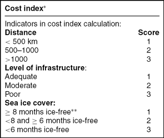
We introduce a cost index based on these indicators in order to evaluate the possible effects that changes in sea ice cover may have on the relative cost of oil development and to compare the oil provinces in 2010 to 2040. The construction of the index is given in Table 1. Sensitivity analysis will be applied to the weights used when aggregating scores to a cost index. Formally we will let a weight restricted Data Envelopment Analysis (DEA) model find optimal weights for the aggregating procedure. A survey of alternative DEA models and applications and weight restrictions of DEA is described in Cooper and others (Reference Cooper, Ruiz, Sirvent, Cooper, Seiford and Zhu2011).
Calculation of cost index
* Scores for all three indicators are given equal weight. In this table the total cost index is the weighted sum of the three indicators when weights are all 1. The effect of other weights are discussed in the paper.
** ‘ice-free’ includes months with less than 10% monthly averaged sea ice covered areas
There are naturally other factors that will affect the speed of oil development in the Arctic such as oil prices, weather conditions and ocean depths. Predicting oil price scenarios for the coming three decades is almost impossible, even though the IEA (2010) expects relative high prices in the future. As such, these variables are excluded from our cost evaluation.
Distances to existing settlements below 500km are assigned the value of one, distances between 500 and 1000km are assigned the value of two, and distances which exceed 1000km are given the value of three. With respect to the level of infrastructure, we evaluate the closest settlement for each province. Provinces with adequate infrastructure are assigned the value 1. The value 2 is assigned to provinces with moderate infrastructure, while those with poor infrastructure capabilities are given the value of 3. Finally, with respect to sea ice cover we proceed as follows. Provinces with less than 10% average sea ice covered areas in eight months or more in one year are given the value 1. Provinces that are ice-free in 6–7 months are assigned the value 2. Provinces that are ice-free less than six months are given the value 3. The values of the three indicators are then added to assign a cost index for each province. In order to show the relative effect of changes in sea ice cover we calculate the cost indices for the given 21 provinces for 2010 and 2040. As infrastructure capabilities are not subject to change in our future projections, the changes which occur are therefore a result of the decline in the sea ice cover. We combine the overall scores into cost level index expressed as a relative percentage score where 1 (100 %) is best cost score, in order to see which provinces will change as a result of the sea ice change.
With respect to sea ice models, in view of the impossibility of including in this paper the projections of the plethora of available models, simulations and emission scenarios for each of the provinces under consideration, our choice went to the NCAR CCSM3 model (Collins and others Reference Collins, Bitz, Blackmon, Bonan, Bretherton, Carton, Chang, Doney, Hack, Henderson, Kiehl, Large, McKenna, Santer and Smith2006), used with success by many research groups, and for which there are accessible and ready to use results from several runs for a large number of climate variables. It also has the advantage of being ‘the median’ of the six global climate models considered in the classic paper by Wang and Overland (Reference Wang and Overland2009).
It should be understood that the simulations from these (and other) respected climate models lead to a wide range of projections for the future of the Arctic sea ice. Some models, such as those developed by the Centre National de Recherches Meteorologiques (CNRM-CM3), the Naval Postgraduate School (NAME) and the Canadian Centre for Climate Model and Analysis (CanESM2), indicate that the Arctic Ocean may be ice-free in the summer before the end of the decade. On the contrary, others, such as the UK Met-Office HadGEM1 or Echo-G, developed in Hamburg, do not rule out the possibility of summer sea ice in the next 40–50 years. As such, the projections that we are about to present about the evolution of the ice cover in each of the provinces must be taken as a rough median of the ensemble of predictions that could be made using all climate models of the literature. The actual future ice conditions may occur up to one or two decades earlier or later than those predicted by the model.
Fig. 2 depicts the projected Arctic sea ice distribution for September based on simulations of the CCSM3 model for the next three decades under the A1B emission scenario and, for comparison, the actual (monthly averaged) situation in September 2010 derived from passive microwave satellite imagery processed with the NASA team algorithm (Markus and Cavalieri Reference Markus and Cavalieri2000; Cavalieri and others Reference Cavalieri, Markus and Comiso2004). Fig. 3 shows analogous projections for the month of March, when the ice cover reaches its annual maximum, and clearly indicates that the changes in the winter ice cover are expected to be much less dramatic than those of the summer.
Sea ice concentrations in September 2010 from satellite observations (top left), and projections by the CCSM3 model for September 2020 (top right), 2030 (bottom left) and 2040 (bottom right) under the A1B emission scenario. Areas of different colours are separated by the 15, 50, 75 and 95% ice concentration contours.
Sea ice concentrations in March 2010 from satellite observations (top left), and projections by the CCSM3 model for March 2020 (top right), 2030 (bottom left) and 2040 (bottom right) under the A1B emission scenario. Areas of different colours are separated by the 15, 50, 75 and 95% ice concentration contours.
While it is important to have an idea of how the global summer sea ice cover will look in the future, our study requires a detailed regional analysis of the future ice conditions in each month of the year. Hence, our objective is to derive the evolution of the ice cover in each of the 21 provinces for the 2010–2040 period under the A1B and A2 scenarios based on the projections of this model for sea ice concentrations. For this purpose, we proceed in the following way. Files with projections from several simulations of the NCAR CCSM3 model for each month between January 2000 and December 2099 are available at the website of the Coupled Model Intercomparison Project (http://esg.llnl.gov. See also Meehl Reference Meehl, Covey, Delworth, Latif, McAvaney, Mitchell, Stouffer and Taylor2007). These files contain the values of several sea ice indicators such as sea ice concentration and mean sea ice thickness for each of the 320×395 cells into which the surface of the Earth is divided. Each cell has dimensions 1.125° in longitude and (at high latitudes) approximately 0.534° in latitude. We start by taking the average of the results of six runs for the A1B scenario and four runs for the A2 scenario. From the sea ice concentrations we can calculate the total sea ice area A of a province P by adding up the sea ice covered areas of each cell (given by the concentration times the area of the cell). In this way we construct a set of 12 time-series, one for each month m, representing the projected evolution of the sea ice covered area of P from 2010 to 2040. We shall denote this time series by Am(y), where y = 2010, 2011, . . ., 2040. These 31 point sequences are, in general, non-monotonic, due not only to decadal and multi-decadal oscillations in the Arctic climate system but also to the interannual variability of the Arctic sea ice, a reflection of short term weather conditions. The latter are the reason for the irregular, sometimes chaotic, appearance of the sequence. The identification of trends in such an irregular time-series is done by calculating A’m(y), the best linear fit of Am(y), using the least squares method. The (almost always negative) gradient of this new linear time-series is what we shall call the rate of decline of the sea ice area in P. This quantity, which we denote by dA’/dt, is indicative of how fast the ice is disappearing in that area. We also assume that the quantities A’m(2010) and A’m(2040) provide realistic quantitative estimates of the amount of ice in each province around 2010 and 2040, respectively.
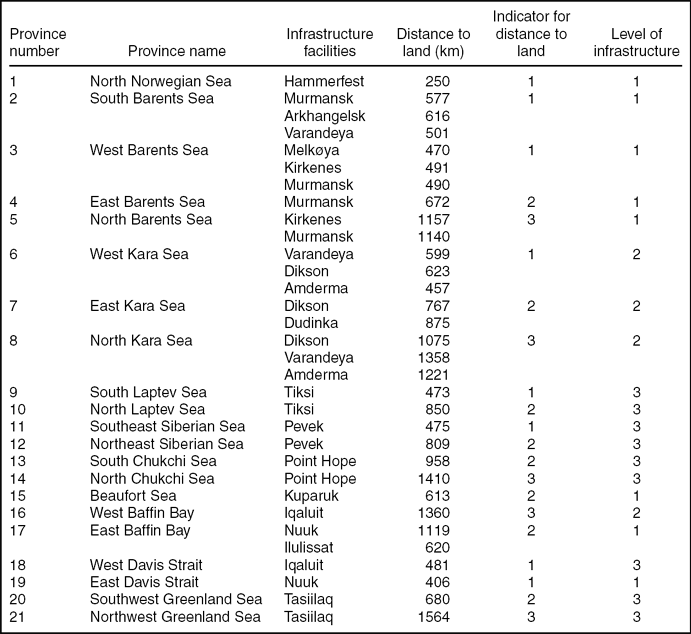
Mean distance and level of infrastructure by provinces
Data and assessments
Sea ice and infrastructure
The levels of costs in the Arctic are relative. They are only comparable within the Arctic, as the general costs of operating in the Arctic far exceed those of other regions of the globe. Even though available data on absolute costs are sparse, and not necessarily accurate, IEA estimates that offshore Arctic production costs including drilling, production facilities and operating and decommissioning components, range from 35 US$ per barrel (IEA 2008) to 100 US$ for the most remote and difficult resources. Production in the Middle East have costs starting at 5 US$ per barrel (The Economist 2012), which highlights the tremendous challenges facing the oil industry in the Arctic. We consider distance to existing infrastructure and sea ice cover as crucial factors in the determination of the relative cost of operating in the Arctic. That does not mean that those are the only factors that will influence future oil activity in the area. Political issues, such as environmental regulations and taxes, will undoubtedly affect the oil industry's willingness to invest. However, it is difficult to predict the political landscape in different countries within the next few decades. For example, Moe and Rowe (Reference Moe, Rowe and Rowe2009) show that Russia, in order to attract offshore investment, is willing to give the ‘finders’ rights to production and development. Nevertheless while Russia has in general the most developed Arctic strategy with adequate infrastructure which includes pipelines and roads, the country is considered high risk with regards to doing business. Russia is not among the top 100 countries for doing business (World Bank 2012). The Russian government is thus on the one side encouraging increased Arctic oil and gas activity, and on the other indirectly constraining development by pursuing policies that are hostile to foreign direct investment.
The remaining Arctic states are among the top 20 for doing business (World Bank 2012). However, changing governments among the western Arctic states pursue different Arctic strategies that make predictions about future policies difficult. The political field in the oil and gas industry is complex, in which the oil companies, government and environmental organizations all are seeking to influence decisions. In some areas environmental concerns have so far triumphed (for example Lofoten and Vesterålen in the north Norwegian Sea), while in others only economic factors are taken into consideration (Arbo and Hersoug Reference Arbo, Hersoug, Arbo and Hersoug2010). It is therefore safe to assume that the increase of activity in the Arctic will vary from region to region due to other factors not included in our cost index.
Thus, in an effort to keep this study realistic, we will not take into account political variables. Tax issues are relevant for a private company making investment decisions. For the general economy, taxing normal profit and resource rent extraction may be considered a redistribution of the wealth generated by exploration of oil and gas resources. Our aim is to study/evaluate the relative cost for 21 Arctic regions, not the distribution of eventual profit among stakeholders. Proximity to existing infrastructure determines a) how easy it becomes to perform exploratory drilling, as it is conditioned by the ability to easily transport material and manpower, and b) field developments and maintenance. Sea ice, on the other hand, determines how difficult it is to operate in an already challenging environment. The amount of sea ice at a given time and the length of the ice season influence both the exploratory drilling and production phase. When ice is present, whether it is permanent, seasonal, or in form of occasional icebergs, the oil industry needs installations that are able to handle those conditions.
With respect to exploratory drilling, seasonal sea ice is a serious obstacle, as the oil companies need two to three months in order to fully be able to complete drilling of the seabed. With regards to the production phase, the amount of sea ice determines what kind of production facilities is needed (Hibernia 2008). While current technology is able to tackle various problems related to sea ice, it is safe to assume that its presence significantly increases the cost of production.
Evaluation of infrastructure, distances, and sea ice conditions
As the distance between settlements and potential oil provinces varies substantially in the Arctic, we have calculated the distances between the oil provinces and the nearest and most developed settlement. We define the distance between a province and a given point on the coast (usually a settlement) as the average distance between the centre of the cells that form that province (described earlier) and the point on the coast.
We define infrastructure of a given province as the fulfillment of one of two conditions. The first is the requirement of at least one settlement with adequate housing, hospital, airport, harbour, and roads in order for the oil industry to easily move exploration and production facilities to that given region. The second condition concerns the existence of facilities directed towards the oil industry, that is, uploading and unloading facilities and/or pipelines. Thus, provinces with adequate infrastructure are given the value 1. Provinces are given the value 2 if the infrastructure capabilities are considered to be medium, while provinces that lack infrastructure are assigned the value 3. The infrastructure measurement remains constant for the period ranging from 2010 to 2040. There are several reasons why future investment in infrastructure is held constant throughout this period. First, predicting investment from various actors is extremely difficult as it is conditioned by variables such as the general state of the global economy. Second, global climate changes may negatively impact current and future infrastructure installations, and could potentially increase the cost of maintenance and construction. It is very difficult to predict how severe the impact may be on infrastructure facilities such as roads and buildings (ACIA 2005). However, some findings suggest that oil and gas related infrastructure may be severely impacted by climate change. Most importantly, the temperature increase affects the Arctic tundra and is likely to have damaging effects on roads and pipelines which are crucial for the hydrocarbon industry. In short, as predicting future investments and the effects of climate change on infrastructure is difficult, we hold, for the purpose of our study, the measurement for infrastructure capabilities for each province constant in 2010 and 2040.
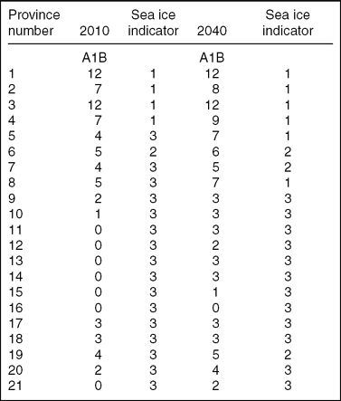
For sea ice we calculate the number of ice-free months per year as shown in Table 3. We define ice-free regions as those with an area with less than 10% ice per month. Provinces with less than 10% ice cover for equal to, or more than 8 months are given the value 1. Provinces that are ice-free in 6–7 months are assigned the value 2. Provinces that are ice-free less than 6 months are given the value 3.
Number of ice-free months per year
Results
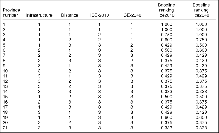
Table 4 gives the results of the calculations of the cost indices. The three indicators of the model are given equals weights and are expressed in a ranking which enables us to study the effects of sea ice change. We recalculate the final cost level index as a relative percentage score where 1 (100%) is best cost score, and the other scores are equally good or less good. The rescaling is done by applying the following formula for each province: New Score Province j = best score in sample/Actual score for province j. The 21 provinces are numbered from 1 to 21 as in Table 4. For region 1(NNS) with cost index score of 3, the relative ranking will be 3/3 = 1, and for 21-NGS the relative ranking will be 3/9 = 0.33.
Inputs and baseline rankings for 2010 and 2040
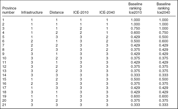
The overall conclusion is that the northern part of Norwegian Sea and the Barents Sea and parts of the Kara Sea will remain the most attractive areas for oil exploration in the coming 30 years. According to the USGS (2008) the probability of finding oil is equally distributed among the oil provinces with the exception of Beaufort Sea. The latter has a higher probability for discovering oil and as this oil province has a cost index of 6 in both 2010 and 2040; the region is interesting in spite of high sea ice coverage. Most of the other provinces do not change relative ranking in the coming 30 years. This implies that the significant part of the region will still pose enormous challenges for the industry. Sea ice will not disappear during the winter, and there is a general lack of well-established settlements. Despite of the presence of sea ice cover, oil companies will most likely continue to search for new potential large scale oil fields. However, sea ice cover will be a significant obstacle to new large scale investments.
In interpreting the results one should bear in mind that the evaluation of the indicators of the cost index in the categories 1, 2 and 3 has been done by the research group based on literature studies and relevant reports. Both changes in the parameter values and relaxing the assignment of equal weighting between indicators in the cost index could change the value of the cost indices and cost levels.
In interpreting the results one should bear in mind that that the indicators of the cost index can take to score values of 1, 2 and 3. The categorization of three levels of scores has been done by the research group based on literature studies and relevant reports. Both changes in the score values and relaxing the assignment of equal weighting between indicators in the cost index could change the value of the cost indices and cost levels.
In this paper we have studied three indicators most relevant to the cost of oil exploration in the Arctic region. Each indicator was assigned a score of three levels, with 1 as the best, 2 as intermediate and 3 as to worst with respect to costs. The cost level of oil producing provinces is then calculated as an equally weighted sum of the scores. Implicitly, the weights are 1 for each indicator when aggregating. The aggregated costs score is a relative score. For 2010 two provinces, North Norwegian Sea and West Barents Sea have achieved the minimum cost score that is the best cost index and two provinces. North Chukchi Sea and North Greenland Sea, have the maximum cost score. For 2040 three provinces have the best cost score. In addition to North Norwegian Sea and West Barents Sea also South Barents Sea has achieved the minimum cost score, which is the best cost index. North Chukchi Sea and North Greenland Sea have achieved the maximum cost score in 2040 and remain the high cost provinces. Five provinces have improved their scores from 2010 to 2040, due to expected changes in in sea ice cover. These provinces are part of the Barents Sea and Kara Sea.
The individual rankings for provinces and variables are our best estimates given available information. We will approach the issue of sensitivity analysis by questioning the weights used to aggregate the scores to a cost index. The cost indices, are admittedly, reasonable but somewhat arbitrary. Therefore the assumption of equal weights is relaxed below.
First, the relevant cost may be the cost difference for the disadvantage of operating in the Arctic, compared to some other place. We find it difficult to construct such a hypothetical cost disadvantage, as we already have made the simplification of using rankings for the disadvantage of distance, and not the actual distance. We do not use actual inputs in the form of cardinal numbers, like distance in kilometers, but have used an ordinal ranking for each input. Notwithstanding, we use relative weights, that may with some discretion be interpreted as relative costs where one cost item is used as a numéraire. Alternative relative weights will be used for the purpose of sensitivity analysis.
The input-oriented multiplier DEA model has been used in many studies when the problem involves restrictions on weights to aggregate input or output, when market prices cannot be used as weights, or prices do not exist. The constant returns to scale input oriented multiplier model is presented as below, for more details see Zhu (Reference Zhu2009).
 \begin{equation*}
Max\sum\limits_{r = 1}^s {u_r y_{ro} }\end{equation*}
Subject to:
 \begin{equation*}
\sum\limits_{i = 1}^m {v_i x_{io} }= 1
\end{equation*}
 \begin{equation*}
\sum\limits_{r = 1}^s {u_r y_{rj} } - \sum\limits_{i = 1}^m {v_i x_{ij} } \le 0\qquad j = 1,\ldots,n\end{equation*}
 \begin{equation*}
u_r, v_i \ge 0\qquad \forall i,r\end{equation*}
Variables to be optimised are ur and vj. In our case s = 1, m = 3, n = 21, and y = 1 for all units. Thus u1 will express the cost efficiency of site ‘o’, and vi (i = 1, 2, 3) are the three weights optimal for maximising cost efficiency for each unit we study.
The model above can be expanded by introducing boundaries for the relative weights v1, v2 and v3. The model with boundaries on relative weights is in the DEA literature called the DEA assurance region model (DEA/AR model for short) and applied in a similar setting as in this paper by Thompson and others (Reference Thompson, Singelton, Thrall and Smith1986), Thompson and others (Reference Thompson, Dharmapala, Thrall, Charnes, Cooper, Lewin and Seiford1994) and Takamura and Tone (Reference Takamura and Tone2003). The baseline results of this paper, as presented in Table 4 as cost level of oil provinces 2010 and 2040 respectively, assume equal relative weights. Formally, equal relative weights for v1, v2 and v3 are formulated as:
1 ≤ v1/v2 ≤ 1
1 ≤ v2/v3 ≤ 1
1 ≤ v3/v1 ≤ 1
For the purpose of sensitivity analyses, we will use two different weight schemes. Weight Scheme 1 is:
0.5 ≤ v1/v2 ≤ 2
0.5 ≤ v2/v3 ≤ 2
0.5 ≤ v3/v1 ≤ 2
Weight scheme 2 builds on Scheme 1, but is less restrictive. We remove the last weight restriction of scheme 1, and keep unchanged the two first restrictions, that is restrictions in Weight Scheme 2 are:
0.5 ≤ v1/v2 ≤ 2
0.5 ≤ v2/v3 ≤ 2
Weight scheme 1 is more restrictive than scheme 2. The calculations are done with infrastructure, distance and ICE-2010 (alternatively ICE-2040) as inputs, first using Weight scheme 1, and then using Weight scheme 2. All together we have tested four combinations of inputs and weight schemes. The results are presented in Table 5 below.
Relative cost rankings for 2010 data based on sequential relaxation of weights
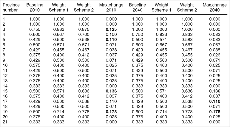
Restricting input weights to be equal will produce the same result as Baseline result 2010 and Baseline result 2040. But equal weights are an extremely restrictive set of weights. When weight restrictions are relaxed, we may experience changes in cost ranking score. The extent of change in cost ranking score is the core of our sensitivity analysis. As weight restrictions are relaxed, relative cost ranking will be either unchanged or better. The improvement from weight Scheme 1 to Scheme 2 is rather minor for the provinces being better ranked.
We use assumptions on ice conditions as given in variable ICE-2010 and ICE-2040, while keeping variables Infrastructure and Distance unchanged. Results are given in Table 5.
The four provinces that are most sensitive to weight relaxation under ICE-2010 are 19-EDS, 15-BEA, 5-NBS, and 3-SBS. Four provinces have unchanged cost score. Under ICE-2040 19-EDS, 17-EBB, and 15-BEA - are most sensitive to relaxation of weights. Five provinces have unchanged cost score from Baseline 2040 when weights are relaxed.
The overall pattern with these experiments with changing weights, as part of a sensitivity analysis, is that there is an overall stability in rankings within the changes in assumptions we have performed. We correlate rankings with increased relaxation of weights, and find that the ranking according to a cost index is generally stable when we allow for relaxation of relative weights.
Relaxation on weights within the limits we have allowed have minimal impact on cost rankings. This gives us confidence in our original ranking of potential oil and gas exploration provinces in the Arctic. The result is also illustrated for ICE-2010 in Fig. 4.
Relative cost ranking for equal weights (Baseline 2010) when compared to Weight Scheme 1 and Weight Scheme 2. Observations are ranked by decreasing Baseline 2010 cost ranking.
Summary and conclusions
The Arctic oil rush has attracted much attention in the last few years. The expectation of increasing development and production in the coming years is shared by a significant number of researchers and commentators (Howard Reference Howard2009; Barents Observer 2010). However, the challenges for the oil industry are formidable. Because of its environment, where it is extremely difficult to operate, the Arctic remains very much a high cost region (IEA 2008).
Our study concluded that, overall, the Arctic sea ice is likely to have a sharp decay (especially in the summer) during the next few decades and that there will be strong regional differences in the pace of the decline. The provinces that exhibit the fastest rate of sea ice decline, evaluated as the change in the numbers of ice-free months per year between 2010 and 2040, are the north Barents Sea, the north Kara Sea, the southeast Siberian Sea, the south Chukchi Sea and the north Chukchi Sea. In all these provinces the number of ice-free months increases by 3, as it can be seen in Table 3 (we have included the north Kara Sea because in the A2 scenario there is also an increase in 3 months from 2010 to 2040). In four of these five regions the biggest jump (two months) will occur between 2030 and 2040. The exception is the south Chukchi Sea, which will increase from 0 to 3 ice-free months between now and 2030. Regions where the number of ice-free months will increase by 2 are the east Barents Sea, the south Laptev Sea (only under the A2 scenario), the north Laptev Sea, the northeast Siberian Sea, and the southwest and northwest Greenland Sea.
In this study we have analysed how three indicators (sea ice, distance to existing settlement, and level of infrastructure) may impact the cost of oil exploration and production. Our results indicate that while certain Arctic provinces may become more attractive during the next 30 years, most provinces will still imply very high costs.
Even though the Arctic is expected to lose a significant portion of its sea ice cover, this does not automatically imply that it will become a substantial oil region. The Arctic may still be a remote region that suffers from the lack of developed settlements; however, this may change depending on state policy and incentives for people to move further north.
Thus, while more attention may be paid to the Arctic as a hydrocarbon producing region in the coming decades, our findings suggest that oil development may not necessarily be substantial in all Arctic provinces. Certain parts of the Arctic may witness a significant increase in activity (Kara Sea, Barents Sea), but these are most likely to be the ones that already have hydrocarbon production today, or where exploration activity is continuing. The sensitivity analysis performed shows that a slightly different cost score will materialise when restrictions on relative weights used for aggregating are relaxed. However, although relative cost scores change, the relative ranking remained almost unchanged. Our results seem to be robust regarding the assumptions used.
Acknowledgement
This work has received funding from the European Union`s Seventh Framework Programme under grant agreement number 226248 – ATP. The authors are also grateful for comments from two anonymous referees.
Appendix. Infrastructure and sea ice in the various Arctic provinces
North Norwegian Sea
Compared to other parts of the Arctic, the coast of northern Norway has highly developed infrastructure. Several small towns along the coast offer several possibilities for the industry. Towns such as Harstad and Tromsø have ports, housing, roads and airports. As a result, several new oil exploration companies, in combination with the establishment of companies that deliver high technology solutions to the industry, use these towns as a base for development. The province is totally free for ice.
West Barents Sea
This part of the Barents Sea is both within Norwegian and Russian jurisdictions, with ports and docks in both countries. Town such as Hammerfest and Kirkenes, and hydrocarbon terminals, such as Melkøya, provide adequate infrastructure. The Norwegian mainland which is in close proximity to the west Barents Sea also includes several small towns, with facilities such as airports, roads, hospitals and housing. In Russia, the town of Murmansk possesses both coastal and offshore oil terminals (AMAP 2007), and a large deep water port. In general Murmansk has a well-developed infrastructure with respect to airports, roads, housing and hospital. It is also the starting point for the road to Norway and Finland.
East, south, north Barents Sea
Murmansk is also the natural centre of activity further into the Russian part of the Barents Sea. A new bridge over Kola Bay, open in 2005, made it possible to reach the isolated parts of the city. Nevertheless the northern and, to some extent, the eastern parts of the Barents Sea are relatively far from the infrastructure capabilities described above.
At present, sea ice in December tends to occur only in the north Barents Sea, covering about 30% of its surface. In the future, however, ice formation is expected to start later and later in the year: by 2020 the December ice cover of the north Barents Sea will be lower than 25% and limited to a band stretching in a W–E direction from Svalbard to Zemlya Frantsa-Iosifa; by 2030 it will be 10–20% and by 2040 only a small fraction (about 5%) of the north Barents Sea will be ice-covered.
It is in the months of January and February that the most significant changes of the next three decades are anticipated. The strong decline forecast for the south Barents Sea in January means that the normal current ice distribution, where about half of the region (usually the White Sea and the areas near the shores) is ice covered, will rapidly evolve towards an ice cover of less than 20% in 30 years time. In the east Barents Sea the ice edge will retreat eastwards towards the west coast of Novaya Zemlya in such a way that by 2020 the ice cover will be on average around 10% and by 2030 almost no ice will exist at this time of the year. But perhaps the most striking changes are expected in the northern sector of the Barents Sea (though, in percentage terms, those in the southern sector are of the same order of magnitude). From now until 2040 (and probably beyond that) there will be a northwards retreat of the ice edge, leading to a continuous increase in the area of open water. By 2020 the ice covered area is still around 40% and ice is most likely to be still present in the region between Svalbard and Zemlya Frantsa-Iosifa. By 2040 the typical January ice cover of the north Barents Sea will be around 20%, the ice edge is likely to be located at around 80°N and consequently the east coast of Svalbard should be ice-free. February and March are the months of maximum ice extent and have similar current and forecast ice distributions, except for the east Barents Sea under the A2 scenario, where the rate of decline for February is projected to be about twice that of March. In the east Barents Sea February is the month of the year where the biggest changes are expected to occur.
Kara Sea
Dikson and Dudenka are towns on the shores of the Kara Sea that possess harbours and airports. Though relatively small, they offer basic infrastructure which may prove useful for further development of offshore oil and gas activity. Varandeya terminal could also become a possible important point for oil and gas production in the Kara Sea (AMAP 2007). This port, though originally related to oil findings in the Pechora Sea, and is connected to existing pipelines, and oil can be offloaded on large tankers able to navigate through ice. Russia's long term plans involve the creation of a transportation corridor by the eastern Ural mountains to the Yamal Peninsula and the Kara Sea (AMAP 2007).
The period of ice formation is the time of the year when the changes are projected for all three sectors of the Kara Sea. Currently ice appears in October in the easternmost waters of the Kara Sea and in the northern area between Zemlya Frantsa-Iosifa and Severnaya Zemlya. November is when large scale freezing really takes place, except in the west Kara which now, is likely to have no ice at all except for some possible fast ice at present near the shores. In the north Kara ice continues to be restricted to the waters between Zemlya Frantsa-Iosifa and Severnaya Zemlya, but in the east Kara, where the ice conditions throughout the year are more severe, there can be already large quantities of ice, especially along the coast of mainland Russia and the west coast of Severnaya Zemlya.
A strong depletion will occur in all three sectors in December with a projected combined rate of decline in sea ice area of 8000 to 9000 km2/year about half of which is for the west Kara Sea. By 2040 the ice cover of the west Kara Sea will go down to 10–20%, with ice being found only in points near the boundary with the east sector. In the east Kara there will be a decline from an almost total ice cover (typically higher than 80%) to less than 60% by the end of the period under study. The ice edge will gradually move eastwards. In the north Kara Sea the ice is expected to almost completely disappear by 2040. There is no ice in the Kara Sea in August and September except possibly in the vicinity of the Severnaya Zemlya straits.
Laptev Sea
There is a general lack of infrastructure on or near the shores of the Laptev Sea. Tiksi possesses an airport and a harbour, in addition to roads and housing which could be used by the oil industry.
Freezing normally begins in October along the shores and the northernmost parts of the Laptev Sea while, at the same time, no ice has yet formed in its central and southern areas. The possibility of ice is greater in the westernmost (high latitude) sector, namely near the east side of the Severnaya Zemlya archipelago or in its straits, where it is not unlikely to find ice that survived the summer melt. However, significant changes in the ice situation at this time of the year are predicted for the next three decades from a current monthly average of 30–40% (50–60%) ice cover in the South (North) Laptev Sea, the situation is expected to evolve to a nearly total absence of ice by 2040. By 2040 freezing is expected to start in November.
From December to April the ice cover is expected to remain total until at least 2040. The breakup of the ice starts in May, and that is not expected to change in the next 30 years: the ice covered area is to remain around 80% in the south Laptev and around 90% in the north Laptev. The evolution of the June ice cover in the next three decades is also predicted to be modest. The current July ice cover of the south Laptev Sea is 35–45% with the bulk of the existing ice likely to be found in the waters southwest of the New Siberian Islands and north of the Taymyr Peninsula, with the possibility of fast ice along the coastline. The north Laptev Sea sector is expected to loose half of its ice between now and 2040, passing from a present situation with two thirds of the region still ice covered in July to one in thirty years’ time in which the ice cover has decreased to about one third. This corresponds to a northwards drift of the ice edge.
East Siberian Sea
Moving further east in Russia there is a general lack of infrastructure on land near to the east Siberian Sea. Pevek is the only settlement that has some infrastructure with facilities such as airports, harbours, roads and housing which could be used by the oil industry. However, according to the AMAP report from 2007, adequate infrastructure does not exist in these regions.
According to the CCSM3 model, the east Siberian Sea is the region of the Arctic that will experience the most extraordinary decline in the amount of sea ice in the autumn. While around 2010 the typical October ice cover is 60–70% in the southern sector and 80–90% in the northern sector. After 2030 it is expected to be regularly below 20% in the southern sector and below 50% in the northern sector with the possibility of years with almost no ice, even in the northern sector. In November the east Siberian Sea is at present totally or almost totally covered with ice but beyond 2030 the ice cover in the southern sector will be 80–90% and around 90% in the north sector.
Between December and April the east Siberian Sea is likely to be permanently ice covered at least until 2040. No significant changes are expected for the month of May, either, with the ice cover to remain in the next three decades just above 90% in the and between 80 and 90% in the southern sector. The projections for the ice situation in June also suggest only a minor decline.
In August, ice covers below 20% in the southeast Siberian Sea begin around 2025 in the A1B scenario and 2035 in A2. After 2030 they are likely to be below 10% in A1B and below 20% in A2.
In September the presence of ice in the north sector is still usual but falling fast, in such a way that after 2020 the ice covered area tends to be between 20 and 30% and after 2030 little or no ice is expected in the region.
Chukchi Sea
The Chukchi sea is within the jurisdiction of both USA and Russia. Point Hope in Alaska offers some basic infrastructure facilities but in general the northwestern part of Alaska is relatively poorly developed compared to the south and areas close to Beaufort Sea. Uelen is the easternmost settlement in Russia and has a cultural centre, a hospital, and a meteorological station. In general, however, there is a lack of adequate infrastructure close to the Chukchi Sea (AMAP 2007).
October is the month with the biggest reduction in the amount of ice. The NCAR model run under the A1B scenario predicts a significant drop in the ice cover of the north Chukchi Sea from the current value of 50–60% (though in some recent years it has been much less than that) to almost nothing around 2040. There is the possibility of the region being totally ice-free as early as the mid–2020s.
A strong decline during the forthcoming decades is predicted for November but there is a lack of agreement between quantitative projections, with the estimates for the total rate of decline going from 4500 km2/year with A2 to 8400 km2/year with A1B. At this time of the year the most relevant changes are in the southern sector. In recent years Bering Strait, the areas south of 70°N and, occasionally, the waters in the central north part of the south Chukchi Sea tend to be still ice-free in the middle of the month. For the north Chukchi Sea we will see a change from an almost total ice cover in November to values of the ice-covered area that can oscillate between 50 and 80% by 2040.
Between December and April the Chukchi Sea is full of ice and this situation is likely to continue in the next decades, with only minor declines of a few per cent anticipated. In June the forecast is for a very small decline in the ice cover of the north Chukchi Sea. In the southern sector the changes will be more rapid, though it is expected that around 2040 the ice cover is still likely to be higher than 50%.
For July, the projections with the A1B scenario are for both sectors to lose half of the ice between now and 2040, while with A2 the changes are more moderate. In August and September there is little or no ice in the south Chukchi Sea while in the north Chukchi the model predicts a sharp decrease in the amount of ice. In September there should be no ice at all in the Chukchi Sea at the end of the period under study whereas in August there is still a possibility of occurrence of ice in the northernmost points.
Beaufort Sea
In Alaska, the mainland close to the Beaufort Sea has some infrastructure facilities. The settlement in Prudhoe Bay contains roads, housing and an airport, whereas the nearby oil field of Kuparuk (near Prudhoe Bay) provides housing for 300 oil workers. In addition there are several dockheads for unloading around the area of Prudhoe Bay. There is, however, a lack of deep water ports (AMAP 2007). Moreover, a pipeline from Valdez in the south to the coast of the Beaufort Sea makes inland transportation a viable option for new production provinces.
Big changes in the ice distribution at the beginning of the freezing season are expected for the next 30 years. October is the month of the year with the steepest projected decline in the amount of sea ice but there are very large discrepancies between the quantitative predictions based on the A1B and the A2 scenarios. In November the ice cover of the Beaufort Sea is now total or almost total and this is expected to remain unchanged until around 2030. However, the model predicts a decline to 70–80% by 2040, when large areas of open water or low ice concentration in the southern half of the region are possible.
From December to April there is compact ice pack all over the Beaufort Sea and that will not change until at least 2040. By the end of May there are the first signs of breakup in the southeast, near the entrance to the Amundsen Gulf. But both the actual and the projected May ice cover for the next three decades is expected to be around 90%. Not much is anticipated to change in June, either, with the ice cover to suffer only a minor decline and remain at around 80% in the next 30 years.
In July, by contrast, significant changes are awaited. By 2040 this contour should be near 76°N, the projections are for a 30–40% ice cover in A1B and 40–50% in A2, and the presence of ice to be limited to the northernmost portions of the Beaufort Sea. The present-day August sea ice area is about 35% with no ice on or near the coasts of Alaska, mainland Canada or Banks Island. By 2040, when the ice area will have dropped to values between 10 and 20%, it should be well beyond 78°N. In September, while nowadays in a normal season there is still some ice that did not melt during the summer, that ice will gradually disappear and by 2040 there should be only minor quantities of ice, if at all, in the Beaufort Sea.
Baffin Bay and Davis Strait
Moving on to the seas off the west coast of Greenland, transport of manpower and relevant equipment for oil and gas exploration is to a large extent dependent on air transport. In this regard the airports of Narsarsauaq and Kangerlussuag are the gateway to Greenland (AMAP 2007). In addition the city of Nuuk, the largest in Greenland, includes harbour, airport, roads, hospitals, hotels.
As a general rule, there is much more ice in the western parts of Davis Strait and Baffin Bay than in the corresponding eastern parts, at any time of the year. We note, for instance, that the ice situations on the west coast of Greenland and the east coast of Baffin Island are quite diverse. Unfortunately, there are discrepancies in what the model takes as starting point (the situation around 2010) and the actually observed ice cover in 2009 and 2010, was much less severe than indicated by the model. As such, it is not completely clear that we can fully trust the projected evolution for this region of the Arctic.
In October, at present times, small amounts of ice can be found in west Davis Strait but only in the northernmost points of the east coast of Baffin Island. In the future, however, the occurrence of ice will become more and more unlikely and at the end of the period under study Davis Strait will have essentially no ice in October. The presence of ice in Baffin Bay at this time of the year is limited to the northwest of the bay. November is the month where the decline in Davis Strait is more abrupt. The eastern part of the strait (and, in particular, the west coast of Greenland) has already little or no ice in current times and the projection is for further reductions. The situation is quite different on the west side of the strait, where ice can currently be found along the coast of Baffin Island north of 65°N and an overall decline from the current value of 55–60% to about 35–40% ice cover is projected for 2040. This reduction corresponds to a westwards migration of the ice edge.
No significant evolution in the ice cover is expected for Baffin Bay until 2040 for the months of December to April, when the ice cover will remain total, or at the time of the break-up, as in May and June. However, in December quantitative changes will occur in the east part of Davis Strait but it is not possible to determine from the projections exactly which areas of the strait are going to have less ice. There is nothing to report about the months of January to May as the ice cover will not change significantly.
Ice can still exist in substantial quantities in the first half of July along the west shores of Baffin Bay and Davis Strait as well as in the northernmost parts of east Baffin Bay (although in recent years the latter has been completely free of ice in July). This situation appears to be possible at any time in the next 30 years but less likely in the future than in present times. In August and September there is fundamentally no ice in Davis Strait or in the eastern half of Baffin Bay. In the west Baffin Bay only a small reduction in ice cover is expected.
West Greenland Sea
The east coast of Greenland has poorly developed infrastructure compared to the west coast. The largest town on the east coast of Greenland is Tasiilaq with almost 2000 inhabitants. It is connected to other towns in Greenland by helicopter. In this paper we shall only consider the western part of the Greenland Sea (as defined in the charts), whose eastern boundary was chosen in such a way that little or no ice can be found at any time of the year east of that line (except at very high latitudes, namely in Fram Strait). We also found that it was desirable to divide the province, somewhat arbitrarily, into southern (SGS) and northern (NGS) sectors. Though neither the eastern part of Fram Strait nor the west or the north coasts of Svalbard are included in region 21 (nor in any of the other regions), it is appropriate do describe the evolution of their sea ice distribution here.
The south Greenland Sea has been almost entirely free of ice in October in recent years but at the end of the m onth ice can already be found in Scoresby Sound and in the waters near the east coast of Greenland at similar latitudes. The projection for the coming decades is for a sharp decrease in the amount of sea ice in the south Greenland Sea in October, a month for which the projected rate of decline is almost double of what is expected for the other months with forecasted substantial changes (the summer months and November). By 2040 the area should contain only small amounts of ice. However, a comparatively large decline is predicted for the south Greenland Sea in the month of November, especially with A1B, corresponding to a migration of the ice concentration contours towards the coast of Greenland.
In December, January and February there will be a noticeable drop in the amount of ice in the south Greenland Sea, especially with the A1B scenario. We note that at present it is possible to find ice in the winter more or less everywhere in Denmark Strait, even in the vicinity of Iceland, that will not be the case in the future, as the ice edge will move westwards towards Greenland and by 2040 sea ice is likely to be restricted to the west half of the strait.
In recent years the south Greenland Sea has already been almost entirely free of ice at the end of June but at the beginning of June it is still possible to find vast quantities of sea ice in the west half of Denmark Strait and along the coast of Greenland north of 65°N. In both scenarios the amount of ice is expected to be reduced by 50% in three decades. Little or no ice exists now in the south Greenland Sea in the months of July, August and September and in the future there should be no ice around, except possibly in some small sheltered areas along the coast of Greenland.