2 Review of the nonlinear quasi-geostrophic balance model

Here we review the derivation of the nonlinear quasi-geostrophic (NQG) balance model (McKiver & Dritschel Reference McKiver and Dritschel2008), which is based on a Rossby-number expansion of the incompressible fluid dynamical equations under the Boussinesq approximation. The starting point is the reformulation introduced by Dritschel & Viúdez (Reference Dritschel and Viúdez2003) that uses the potential vorticity (PV) alongside a pair of ‘thermal–wind imbalance’ variables as the prognostic variables, rather than the standard velocity components and density. The first prognostic equation expresses the material conservation of PV, or its anomaly $\unicode[STIX]{x1D71B}$ , with respect to a constant background value:

(2.1) $$\begin{eqnarray}\frac{\text{D}\unicode[STIX]{x1D71B}}{\text{D}t}\equiv \unicode[STIX]{x1D71B}_{t}+\boldsymbol{u}\boldsymbol{\cdot }\unicode[STIX]{x1D735}\unicode[STIX]{x1D71B}=0.\end{eqnarray}$$

Here a subscript $t$ denotes partial differentiation with respect to time, $\boldsymbol{u}=(u,v,w)$ is the velocity field, and the (dimensionless) PV anomaly $\unicode[STIX]{x1D71B}$ is defined as

(2.2) $$\begin{eqnarray}\unicode[STIX]{x1D71B}\equiv \frac{\unicode[STIX]{x1D701}}{f}+\frac{b_{z}}{N^{2}}+\frac{\unicode[STIX]{x1D74E}\boldsymbol{\cdot }\unicode[STIX]{x1D735}b}{fN^{2}},\end{eqnarray}$$

where $\unicode[STIX]{x1D74E}$ is the relative vorticity, with $\unicode[STIX]{x1D701}$ being its vertical component, $b$ is the buoyancy anomaly (see below), while $f$ and $N$ are the Coriolis and buoyancy frequencies, respectively, both assumed to be constant. Throughout, subscripts $x$ , $y$ and $z$ on fields denote partial differentiation. The total buoyancy is related to the density $\unicode[STIX]{x1D70C}$ by $\bar{b}(z)+b(\boldsymbol{x},t)=-g(\unicode[STIX]{x1D70C}-\unicode[STIX]{x1D70C}_{0})/\unicode[STIX]{x1D70C}_{0}$ , where $g$ is the acceleration due to gravity and $\unicode[STIX]{x1D70C}_{0}$ is the mean density. The part depending only on $z$ is taken to be a linear function, $\bar{b}(z)=N^{2}z$ , without loss of generality. The two other prognostic variables used are the horizontal components of the (dimensionless) ageostrophic vorticity, defined as

(2.3) $$\begin{eqnarray}\mathscr{A}\equiv (A,B,C)=\unicode[STIX]{x1D74E}/f+\unicode[STIX]{x1D735}b/f^{2}.\end{eqnarray}$$

The horizontal components $(A,B)$ essentially express the departure from thermal–wind (geostrophic–hydrostatic) balance. Their time evolution is given by

(2.4a ) $$\begin{eqnarray}\displaystyle & \displaystyle \frac{\text{D}A}{\text{D}t}=fB+(1-\unicode[STIX]{x1D712}^{2})w_{x}+f^{-1}\unicode[STIX]{x1D74E}\boldsymbol{\cdot }\unicode[STIX]{x1D735}u-f^{-2}\boldsymbol{u}_{x}\boldsymbol{\cdot }\unicode[STIX]{x1D735}b, & \displaystyle\end{eqnarray}$$

(2.4b ) $$\begin{eqnarray}\displaystyle & \displaystyle \frac{\text{D}B}{\text{D}t}=-fA+(1-\unicode[STIX]{x1D712}^{2})w_{y}+f^{-1}\unicode[STIX]{x1D74E}\boldsymbol{\cdot }\unicode[STIX]{x1D735}v-f^{-2}\boldsymbol{u}_{y}\boldsymbol{\cdot }\unicode[STIX]{x1D735}b, & \displaystyle\end{eqnarray}$$

$\unicode[STIX]{x1D712}\equiv N/f$

The NQG balance equations are derived from (2.2) and (2.4) by performing an expansion in the PV-based Rossby number, $\unicode[STIX]{x1D716}=|\unicode[STIX]{x1D71B}|_{\mathit{max}}$ , up to second order. The thermal–wind imbalance variables scale like $\unicode[STIX]{x1D716}^{2}$ . Hence the horizontal components of the ageostrophic vorticity vanish at $O(\unicode[STIX]{x1D716})$ and only the linear terms remain in the definition of PV (2.2), i.e.

(2.5) $$\begin{eqnarray}\frac{\unicode[STIX]{x1D701}^{1}}{f}+\frac{b_{z}^{1}}{N^{2}}=\unicode[STIX]{x1D71B}.\end{eqnarray}$$

Here and below, numerical superscripts on field variables only denote order in Rossby number. At $O(\unicode[STIX]{x1D716}^{2})$ quadratic terms appear in both (2.4) and (2.2) involving the first-order variables, i.e.

(2.6a ) $$\begin{eqnarray}\displaystyle & \displaystyle B^{2}+\frac{(1-\unicode[STIX]{x1D712}^{2})}{f}w_{x}^{2}=-\frac{1}{f^{2}}\left[\unicode[STIX]{x1D74E}^{1}\boldsymbol{\cdot }\unicode[STIX]{x1D735}u^{1}-\frac{1}{f}\boldsymbol{u}_{x}^{1}\boldsymbol{\cdot }\unicode[STIX]{x1D735}b^{1}\right], & \displaystyle\end{eqnarray}$$

(2.6b ) $$\begin{eqnarray}\displaystyle & \displaystyle A^{2}-\frac{(1-\unicode[STIX]{x1D712}^{2})}{f}w_{y}^{2}=\frac{1}{f^{2}}\left[\unicode[STIX]{x1D74E}^{1}\boldsymbol{\cdot }\unicode[STIX]{x1D735}v^{1}-\frac{1}{f}\boldsymbol{u}_{y}^{1}\boldsymbol{\cdot }\unicode[STIX]{x1D735}b^{1}\right], & \displaystyle\end{eqnarray}$$

(2.6c ) $$\begin{eqnarray}\displaystyle & \displaystyle \frac{\unicode[STIX]{x1D701}^{2}}{f}+\frac{b_{z}^{2}}{N^{2}}=-\frac{\unicode[STIX]{x1D74E}^{1}\boldsymbol{\cdot }\unicode[STIX]{x1D735}b^{1}}{fN^{2}}. & \displaystyle\end{eqnarray}$$

$\unicode[STIX]{x1D753}\equiv (\unicode[STIX]{x1D711},\unicode[STIX]{x1D713},\unicode[STIX]{x1D719})$

$\unicode[STIX]{x1D753}$

(2.7) $$\begin{eqnarray}\displaystyle & \displaystyle \boldsymbol{u}=-f\unicode[STIX]{x1D735}\times \unicode[STIX]{x1D753}, & \displaystyle\end{eqnarray}$$

(2.8) $$\begin{eqnarray}\displaystyle & \displaystyle b=N^{2}(\unicode[STIX]{x1D711}_{x}+\unicode[STIX]{x1D713}_{y})+f^{2}\unicode[STIX]{x1D719}_{z}. & \displaystyle\end{eqnarray}$$

Now if we transform to a coordinate frame where the $z$ -axis is stretched by $\unicode[STIX]{x1D712}\equiv N/f$ and substitute the vector potential $\unicode[STIX]{x1D753}$ into the NQG equations (2.5) and (2.6), we obtain the QG equations at $O(\unicode[STIX]{x1D716})$ ,

(2.9) $$\begin{eqnarray}\unicode[STIX]{x1D6FB}^{2}\unicode[STIX]{x1D719}^{1}=\unicode[STIX]{x1D71B},\end{eqnarray}$$

and at $O(\unicode[STIX]{x1D716}^{2})$ ,

(2.10a ) $$\begin{eqnarray}\displaystyle & \displaystyle \unicode[STIX]{x1D6FB}^{2}\unicode[STIX]{x1D711}^{2}=\frac{2}{\unicode[STIX]{x1D712}}(\unicode[STIX]{x1D719}_{yy}^{1}\unicode[STIX]{x1D719}_{zx}^{1}-\unicode[STIX]{x1D719}_{yz}^{1}\unicode[STIX]{x1D719}_{xy}^{1}), & \displaystyle\end{eqnarray}$$

(2.10b ) $$\begin{eqnarray}\displaystyle & \displaystyle \unicode[STIX]{x1D6FB}^{2}\unicode[STIX]{x1D713}^{2}=\frac{2}{\unicode[STIX]{x1D712}}(\unicode[STIX]{x1D719}_{xx}^{1}\unicode[STIX]{x1D719}_{yz}^{1}-\unicode[STIX]{x1D719}_{zx}^{1}\unicode[STIX]{x1D719}_{xy}^{1}), & \displaystyle\end{eqnarray}$$

(2.10c ) $$\begin{eqnarray}\displaystyle & \displaystyle \unicode[STIX]{x1D6FB}^{2}\unicode[STIX]{x1D719}^{2}=|\unicode[STIX]{x1D735}\unicode[STIX]{x1D719}_{z}^{1}|^{2}-(\unicode[STIX]{x1D6FB}^{2}\unicode[STIX]{x1D719}^{1})\unicode[STIX]{x1D719}_{zz}^{1}. & \displaystyle\end{eqnarray}$$

$b$

3 Review of the quasi-geostrophic ellipsoidal vortex

Next we review the solutions to the first-order part of the NQG equations, i.e. the QG equations, in the case of a single ellipsoid of uniform potential vorticity centred at the origin with axis half-lengths $a\leqslant b\leqslant c$ . The unit vectors $\hat{\boldsymbol{a}}$ , $\hat{\boldsymbol{b}}$ and $\hat{\boldsymbol{c}}$ directed along these axes may be written

(3.1a-c ) $$\begin{eqnarray}\hat{\boldsymbol{a}}=\left(\begin{array}{@{}c@{}}\hat{a}_{1}\\ \hat{a}_{2}\\ \hat{a}_{3}\end{array}\right)\!,\quad \hat{\boldsymbol{b}}=\left(\begin{array}{@{}c@{}}\hat{b}_{1}\\ \hat{b}_{2}\\ \hat{b}_{3}\end{array}\right)\!,\quad \hat{\boldsymbol{c}}=\left(\begin{array}{@{}c@{}}{\hat{c}}_{1}\\ {\hat{c}}_{2}\\ {\hat{c}}_{3}\end{array}\right)\!.\end{eqnarray}$$

Following the formulation of McKiver & Dritschel (Reference McKiver and Dritschel2003), the shape and orientation of the vortex are encapsulated in a single symmetric $3\times 3$ matrix $\unicode[STIX]{x1D63D}$ defined by

(3.2) $$\begin{eqnarray}\unicode[STIX]{x1D63D}=a^{2}\hat{\boldsymbol{a}}\hat{\boldsymbol{a}}^{\text{T}}+b^{2}\hat{\boldsymbol{b}}\hat{\boldsymbol{b}}^{\text{T}}+c^{2}\hat{\boldsymbol{c}}\hat{\boldsymbol{c}}^{\text{T}},\end{eqnarray}$$

where the superscript T denotes transpose. From this matrix, the axis lengths and orientation vectors can be determined from the solution of the eigenvalue problem:

(3.3a ) $$\begin{eqnarray}\displaystyle & \unicode[STIX]{x1D63D}\hat{\boldsymbol{a}}=a^{2}\hat{\boldsymbol{a}}, & \displaystyle\end{eqnarray}$$

(3.3b ) $$\begin{eqnarray}\displaystyle & \unicode[STIX]{x1D63D}\hat{\boldsymbol{b}}=b^{2}\hat{\boldsymbol{b}}, & \displaystyle\end{eqnarray}$$

(3.3c ) $$\begin{eqnarray}\displaystyle & \unicode[STIX]{x1D63D}\hat{\boldsymbol{c}}=c^{2}\hat{\boldsymbol{c}}. & \displaystyle\end{eqnarray}$$

(3.4) $$\begin{eqnarray}\boldsymbol{u}=\unicode[STIX]{x1D64E}\boldsymbol{x},\end{eqnarray}$$

where $\unicode[STIX]{x1D64E}$ depends only on time $t$ (we refer to $\unicode[STIX]{x1D64E}$ as the flow matrix subsequently), then the equation of motion for the ellipsoid is simply

(3.5) $$\begin{eqnarray}\frac{\text{d}\unicode[STIX]{x1D63D}}{\text{d}t}=\unicode[STIX]{x1D64E}\unicode[STIX]{x1D63D}+\unicode[STIX]{x1D63D}\unicode[STIX]{x1D64E}^{\text{T}}\end{eqnarray}$$

(McKiver & Dritschel Reference McKiver and Dritschel2003). The elements of the flow matrix depend on the governing system of fluid dynamical equations. Notably, the only requirement is that the flow field within the ellipsoid has linear spatial dependence – this preserves the ellipsoidal form.

To obtain an ellipsoidal solution for the NQG equations, we need to show that the interior flow field is linear and calculate the flow matrix $\unicode[STIX]{x1D64E}$ to $O(\unicode[STIX]{x1D716}^{2})$ . At first order in Rossby number $\unicode[STIX]{x1D716}$ , the NQG balance equations derived in the previous section reduce to quasi-geostrophic balance (2.9), found simply by inverting

(3.6) $$\begin{eqnarray}\unicode[STIX]{x1D6FB}^{2}\unicode[STIX]{x1D719}_{I}^{1}=Q_{\unicode[STIX]{x1D719}}^{1},\end{eqnarray}$$

for the interior vertical component of the potential $\unicode[STIX]{x1D719}_{I}^{1}$ , where the source term is the (unexpanded) PV anomaly, i.e.  $Q_{\unicode[STIX]{x1D719}}^{1}=\unicode[STIX]{x1D71B}$ . The solution to this Poisson equation must match the solution $\unicode[STIX]{x1D719}_{E}^{1}$ external to the ellipsoid where the PV anomaly is zero, i.e.

(3.7) $$\begin{eqnarray}\unicode[STIX]{x1D6FB}^{2}\unicode[STIX]{x1D719}_{E}^{1}=0.\end{eqnarray}$$

These equations have a known analytical solution for the inner and outer fields. The inner field is given by (omitting the constant term)

(3.8) $$\begin{eqnarray}\unicode[STIX]{x1D719}_{I}^{1}={\textstyle \frac{1}{2}}\boldsymbol{x}^{\text{T}}\unicode[STIX]{x1D731}_{I}^{1}\boldsymbol{x},\end{eqnarray}$$

where $\unicode[STIX]{x1D731}_{I}^{1}$ is the $3\times 3$ symmetric matrix

(3.9) $$\begin{eqnarray}\unicode[STIX]{x1D731}_{I}^{1}=\unicode[STIX]{x1D709}_{a}\hat{\boldsymbol{a}}\hat{\boldsymbol{a}}^{\text{T}}+\unicode[STIX]{x1D709}_{b}\hat{\boldsymbol{b}}\hat{\boldsymbol{b}}^{\text{T}}+\unicode[STIX]{x1D709}_{c}\hat{\boldsymbol{c}}\hat{\boldsymbol{c}}^{\text{T}}.\end{eqnarray}$$

The coefficients $\unicode[STIX]{x1D709}_{a}$ , $\unicode[STIX]{x1D709}_{b}$ and $\unicode[STIX]{x1D709}_{c}$ are given by

(3.10a ) $$\begin{eqnarray}\displaystyle & \unicode[STIX]{x1D709}_{a}=\unicode[STIX]{x1D705}_{v}R_{D}(b^{2},c^{2},a^{2}), & \displaystyle\end{eqnarray}$$

(3.10b ) $$\begin{eqnarray}\displaystyle & \unicode[STIX]{x1D709}_{b}=\unicode[STIX]{x1D705}_{v}R_{D}(c^{2},a^{2},b^{2}), & \displaystyle\end{eqnarray}$$

(3.10c ) $$\begin{eqnarray}\displaystyle & \unicode[STIX]{x1D709}_{c}=\unicode[STIX]{x1D705}_{v}R_{D}(a^{2},b^{2},c^{2}), & \displaystyle\end{eqnarray}$$

(3.11) $$\begin{eqnarray}\unicode[STIX]{x1D705}_{v}=\frac{\unicode[STIX]{x1D71B}abc}{3}\end{eqnarray}$$

and where $R_{D}$ is the elliptic integral of the second kind defined by

(3.12) $$\begin{eqnarray}R_{D}(f,g,h)\equiv \frac{3}{2}\int _{0}^{\infty }\frac{\text{d}t}{\sqrt{(t+f)(t+g)(t+h)^{3}}}.\end{eqnarray}$$

The outer solution has the same form, i.e.

(3.13) $$\begin{eqnarray}\unicode[STIX]{x1D719}_{E}^{1}={\textstyle \frac{1}{2}}\boldsymbol{x}^{\text{T}}\unicode[STIX]{x1D731}_{E}^{1}\boldsymbol{x},\end{eqnarray}$$

but now the matrix $\unicode[STIX]{x1D731}_{E}^{1}$ is given by

(3.14) $$\begin{eqnarray}\unicode[STIX]{x1D731}_{E}^{1}=\unicode[STIX]{x1D709}_{\unicode[STIX]{x1D6FC}}\hat{\boldsymbol{a}}\hat{\boldsymbol{a}}^{\text{T}}+\unicode[STIX]{x1D709}_{\unicode[STIX]{x1D6FD}}\hat{\boldsymbol{b}}\hat{\boldsymbol{b}}^{\text{T}}+\unicode[STIX]{x1D709}_{\unicode[STIX]{x1D6FE}}\hat{\boldsymbol{c}}\hat{\boldsymbol{c}}^{\text{T}},\end{eqnarray}$$

where

(3.15a ) $$\begin{eqnarray}\displaystyle & \unicode[STIX]{x1D709}_{\unicode[STIX]{x1D6FC}}=\unicode[STIX]{x1D705}_{v}R_{D}(\unicode[STIX]{x1D6FD}^{2},\unicode[STIX]{x1D6FE}^{2},\unicode[STIX]{x1D6FC}^{2}), & \displaystyle\end{eqnarray}$$

(3.15b ) $$\begin{eqnarray}\displaystyle & \unicode[STIX]{x1D709}_{\unicode[STIX]{x1D6FD}}=\unicode[STIX]{x1D705}_{v}R_{D}(\unicode[STIX]{x1D6FE}^{2},\unicode[STIX]{x1D6FC}^{2},\unicode[STIX]{x1D6FD}^{2}), & \displaystyle\end{eqnarray}$$

(3.15c ) $$\begin{eqnarray}\displaystyle & \unicode[STIX]{x1D709}_{\unicode[STIX]{x1D6FE}}=\unicode[STIX]{x1D705}_{v}R_{D}(\unicode[STIX]{x1D6FC}^{2},\unicode[STIX]{x1D6FD}^{2},\unicode[STIX]{x1D6FE}^{2}), & \displaystyle\end{eqnarray}$$

$\unicode[STIX]{x1D6FC}^{2}=a^{2}+\unicode[STIX]{x1D706}$

$\unicode[STIX]{x1D6FD}^{2}=b^{2}+\unicode[STIX]{x1D706}$

$\unicode[STIX]{x1D6FE}^{2}=c^{2}+\unicode[STIX]{x1D706}$

$\unicode[STIX]{x1D706}$

(3.16) $$\begin{eqnarray}\boldsymbol{x}^{\text{T}}\unicode[STIX]{x1D63C}\boldsymbol{x}=1,\end{eqnarray}$$

where

(3.17) $$\begin{eqnarray}\unicode[STIX]{x1D63C}=\frac{\hat{\boldsymbol{a}}\hat{\boldsymbol{a}}^{\text{T}}}{a^{2}+\unicode[STIX]{x1D706}}+\frac{\hat{\boldsymbol{b}}\hat{\boldsymbol{b}}^{\text{T}}}{b^{2}+\unicode[STIX]{x1D706}}+\frac{\hat{\boldsymbol{c}}\hat{\boldsymbol{c}}^{\text{T}}}{c^{2}+\unicode[STIX]{x1D706}}.\end{eqnarray}$$

Note that $\unicode[STIX]{x1D706}=0$ corresponds to the boundary of the ellipsoid. Since the velocity field at $O(\unicode[STIX]{x1D716})$ is given by $(u,v,w)=(-\unicode[STIX]{x2202}\unicode[STIX]{x1D719}_{I}^{1}/\unicode[STIX]{x2202}y,\unicode[STIX]{x2202}\unicode[STIX]{x1D719}_{I}^{1}/\unicode[STIX]{x2202}x,0)$ , it depends linearly on the spatial coordinates and so satisfies the evolution equation for the ellipsoid, equation (3.5). This solution for the uniform ellipsoid was in fact originally derived by Laplace (Reference Laplace1784) for gravitating bodies with uniform mass. It was more recently applied by Meacham (Reference Meacham1992) to the case of an ellipsoidal vortex in quasi-geostrophic flow. In general this solution applies when the Laplacian of some potential is equal to a uniform source term within the ellipsoid but a zero source term outside. When this is the case, the inner and outer solutions (the outer solution can be expanded in a series of ellipsoidal harmonics; see appendix A) for the vertical potential and its gradient can be matched at the boundary, as was done for the QG ellipsoidal vortex by Meacham (Reference Meacham1992). The solution derived by Laplace (Reference Laplace1784) however is more general.

Given then the solution for the flow field, the flow matrix is given by

(3.18) $$\begin{eqnarray}\unicode[STIX]{x1D64E}^{1}=\unicode[STIX]{x1D647}_{\unicode[STIX]{x1D719}}\unicode[STIX]{x1D731}_{I}^{1},\end{eqnarray}$$

where the skew matrix

(3.19) $$\begin{eqnarray}\unicode[STIX]{x1D647}_{\unicode[STIX]{x1D719}}=\left(\begin{array}{@{}ccc@{}}0 & -1 & 0\\ 1 & 0 & 0\\ 0 & 0 & 0\end{array}\right)\end{eqnarray}$$

arises from the special form of the QG velocity field.

4 Balanced ellipsoidal vortex

4.1 Homogeneous solution

We next consider the NQG equations at $O(\unicode[STIX]{x1D716}^{2})$ for the ellipsoidal vortex. Unlike the case of the QG equations above, where there is a single streamfunction determining the flow field, the next order in NQG balance requires the full vector potential, $\unicode[STIX]{x1D753}=(\unicode[STIX]{x1D711},\unicode[STIX]{x1D713},\unicode[STIX]{x1D719})$ . If we substitute the first-order solutions $\unicode[STIX]{x1D719}^{1}$ in the equations at the next order, i.e. in (2.10), we can obtain the following equations for the interior potentials (after some manipulation):

(4.1a ) $$\begin{eqnarray}\displaystyle & \displaystyle \unicode[STIX]{x1D6FB}^{2}\unicode[STIX]{x1D711}_{I}^{2}=Q_{\unicode[STIX]{x1D711}}^{2}=-\frac{2}{\unicode[STIX]{x1D712}}(\unicode[STIX]{x1D709}_{b}\unicode[STIX]{x1D709}_{c}\hat{a}_{3}\hat{a}_{1}+\unicode[STIX]{x1D709}_{c}\unicode[STIX]{x1D709}_{a}\hat{b}_{3}\hat{b}_{1}+\unicode[STIX]{x1D709}_{a}\unicode[STIX]{x1D709}_{b}{\hat{c}}_{3}{\hat{c}}_{1}), & \displaystyle\end{eqnarray}$$

(4.1b ) $$\begin{eqnarray}\displaystyle & \displaystyle \unicode[STIX]{x1D6FB}^{2}\unicode[STIX]{x1D713}_{I}^{2}=Q_{\unicode[STIX]{x1D713}}^{2}=-\frac{2}{\unicode[STIX]{x1D712}}(\unicode[STIX]{x1D709}_{b}\unicode[STIX]{x1D709}_{c}\hat{a}_{2}\hat{a}_{3}+\unicode[STIX]{x1D709}_{c}\unicode[STIX]{x1D709}_{a}\hat{b}_{2}\hat{b}_{3}+\unicode[STIX]{x1D709}_{a}\unicode[STIX]{x1D709}_{b}{\hat{c}}_{2}{\hat{c}}_{3}), & \displaystyle\end{eqnarray}$$

(4.1c ) $$\begin{eqnarray}\displaystyle & \unicode[STIX]{x1D6FB}^{2}\unicode[STIX]{x1D719}_{I}^{2}=Q_{\unicode[STIX]{x1D719}}^{2}=-\unicode[STIX]{x1D709}_{a}(\unicode[STIX]{x1D709}_{b}+\unicode[STIX]{x1D709}_{c})\hat{a}_{3}^{2}-\unicode[STIX]{x1D709}_{b}(\unicode[STIX]{x1D709}_{c}+\unicode[STIX]{x1D709}_{a})\hat{b}_{3}^{2}-\unicode[STIX]{x1D709}_{c}(\unicode[STIX]{x1D709}_{a}+\unicode[STIX]{x1D709}_{b}){\hat{c}}_{3}^{2}. & \displaystyle\end{eqnarray}$$

The source terms on the right-hand sides, while complicated combinations of elliptic integrals and axes vector components, are spatially independent and at any instantaneous time they are uniform within the ellipsoidal vortex. However, unlike the case of the QG vortex, these source terms do not vanish outside the vortex. In fact, these source terms can be extremely complicated, mainly because of the dependence of the elliptic integral coefficients, $\unicode[STIX]{x1D709}_{\unicode[STIX]{x1D6FC}}$ , $\unicode[STIX]{x1D709}_{\unicode[STIX]{x1D6FD}}$ and $\unicode[STIX]{x1D709}_{\unicode[STIX]{x1D6FE}}$ , on the spatial coordinates (see appendices B and C).

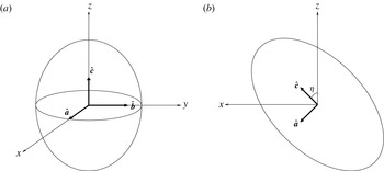
In appendix D we derive the exterior source terms for the special case of an ellipsoid in ‘standard position’, where the coordinate axes are aligned with the axes of the ellipsoid (see figure 1 a). The full analytical solution in this case is presented in the next subsection. In the general case of an arbitrarily oriented ellipsoid, however, the analysis appears to be prohibitively complicated due to the exceedingly complex forms of the exterior source terms. If one considers the case of a spherical vortex, i.e.  $a=b=c$ , the magnitude of these source terms can be estimated to be $O(\unicode[STIX]{x1D71B}^{2}/r^{6})$ , where $r$ is the radial distance from the centre of the vortex. The small size of these terms together with their rapid decay may explain why, in practice, they contribute so weakly to the full solution (as shown below in § 4.2.2).

Figure 1.

Schematic of the ellipsoidal vortex in two configurations: (a) standard position with the ellipsoidal axis ( $\hat{\boldsymbol{a}},\hat{\boldsymbol{b}},\hat{\boldsymbol{c}}$ ) aligned with the coordinate axis ( $x,y,z$ ), and (b) spheroidal vortex tilted by an angle $\unicode[STIX]{x1D702}$ about the $y$ -axis.

To make progress in the general case, we make an approximation that vastly simplifies the analysis: we simply neglect the exterior source terms. The accuracy of the homogeneous solution thereby obtained is tested in the next section, comparing it to both the full analytical solution as well as to the full iterative NQG balance solution (found numerically).

Setting the exterior source terms to zero allows us to apply directly Laplace’s solution to the equations (4.1) to get

(4.2a ) $$\begin{eqnarray}\displaystyle & \unicode[STIX]{x1D711}^{2}={\textstyle \frac{1}{2}}\boldsymbol{x}^{\text{T}}\unicode[STIX]{x1D71E}_{I}^{2}\boldsymbol{x}, & \displaystyle\end{eqnarray}$$

(4.2b ) $$\begin{eqnarray}\displaystyle & \unicode[STIX]{x1D713}^{2}={\textstyle \frac{1}{2}}\boldsymbol{x}^{\text{T}}\unicode[STIX]{x1D733}_{I}^{2}\boldsymbol{x}, & \displaystyle\end{eqnarray}$$

(4.2c ) $$\begin{eqnarray}\displaystyle & \unicode[STIX]{x1D719}^{2}={\textstyle \frac{1}{2}}\boldsymbol{x}^{\text{T}}\unicode[STIX]{x1D731}_{I}^{2}\boldsymbol{x}, & \displaystyle\end{eqnarray}$$

where $\unicode[STIX]{x1D71E}_{I}^{2}$ , $\unicode[STIX]{x1D733}_{I}^{2}$ and $\unicode[STIX]{x1D731}_{I}^{2}$ are $3\times 3$ matrices given by

(4.3a ) $$\begin{eqnarray}\displaystyle & \displaystyle \unicode[STIX]{x1D71E}_{I}^{2}=\frac{Q_{\unicode[STIX]{x1D711}}^{2}}{\unicode[STIX]{x1D71B}}\unicode[STIX]{x1D731}^{1}, & \displaystyle\end{eqnarray}$$

(4.3b ) $$\begin{eqnarray}\displaystyle & \displaystyle \unicode[STIX]{x1D733}_{I}^{2}=\frac{Q_{\unicode[STIX]{x1D713}}^{2}}{\unicode[STIX]{x1D71B}}\unicode[STIX]{x1D731}^{1}, & \displaystyle\end{eqnarray}$$

(4.3c ) $$\begin{eqnarray}\displaystyle & \displaystyle \unicode[STIX]{x1D731}_{I}^{2}=\frac{Q_{\unicode[STIX]{x1D719}}^{2}}{\unicode[STIX]{x1D71B}}\unicode[STIX]{x1D731}^{1}. & \displaystyle\end{eqnarray}$$

These solutions are second order in the PV anomaly $\unicode[STIX]{x1D71B}$ and hence in the Rossby number $\unicode[STIX]{x1D716}$ . As the interior potentials have a quadratic dependence on spatial coordinates, the self-induced velocity field is linear and preserves the ellipsoidal form. Thus, we can calculate the flow matrix using the definition of the velocity, equation (2.7), which can be written as

(4.4) $$\begin{eqnarray}\unicode[STIX]{x1D64E}^{2}=\unicode[STIX]{x1D647}_{\unicode[STIX]{x1D711}}\unicode[STIX]{x1D71E}_{I}^{2}+\unicode[STIX]{x1D647}_{\unicode[STIX]{x1D713}}\unicode[STIX]{x1D733}_{I}^{2}+\unicode[STIX]{x1D647}_{\unicode[STIX]{x1D719}}\unicode[STIX]{x1D731}_{I}^{2},\end{eqnarray}$$

where the skew matrices are defined as

(4.5a-c ) $$\begin{eqnarray}\unicode[STIX]{x1D647}_{\unicode[STIX]{x1D711}}=\left(\begin{array}{@{}ccc@{}}0 & 0 & 0\\ 0 & 0 & -\unicode[STIX]{x1D712}\\ 0 & 1 & 0\end{array}\right)\!,\quad \unicode[STIX]{x1D647}_{\unicode[STIX]{x1D713}}=\left(\begin{array}{@{}ccc@{}}0 & 0 & \unicode[STIX]{x1D712}\\ 0 & 0 & 0\\ -1 & 0 & 0\end{array}\right)\!,\quad \unicode[STIX]{x1D647}_{\unicode[STIX]{x1D719}}=\left(\begin{array}{@{}ccc@{}}0 & -1 & 0\\ 1 & 0 & 0\\ 0 & 0 & 0\end{array}\right)\!,\end{eqnarray}$$

and where the scaling factor $\unicode[STIX]{x1D712}=N/f$ arises where the velocity field depends on $z$ derivatives of the vector potential components. Thus the general flow matrix up to $O(\unicode[STIX]{x1D716}^{2})$ can be written as

(4.6) $$\begin{eqnarray}\unicode[STIX]{x1D64E}=\frac{1}{\unicode[STIX]{x1D71B}}(Q_{\unicode[STIX]{x1D711}}\unicode[STIX]{x1D647}_{\unicode[STIX]{x1D711}}+Q_{\unicode[STIX]{x1D713}}\unicode[STIX]{x1D647}_{\unicode[STIX]{x1D713}}+Q_{\unicode[STIX]{x1D719}}\unicode[STIX]{x1D647}_{\unicode[STIX]{x1D719}})\unicode[STIX]{x1D731}^{1},\end{eqnarray}$$

where the source terms $(Q_{\unicode[STIX]{x1D711}},Q_{\unicode[STIX]{x1D713}},Q_{\unicode[STIX]{x1D719}})$ are the sum of the first- and second-order source terms defined in (3.6) and (4.1), respectively (note that at first order $Q_{\unicode[STIX]{x1D711}}^{1}=Q_{\unicode[STIX]{x1D713}}^{1}=0$ ).

4.2 Particular solutions

4.2.1 The ellipsoid in standard position

We now derive the complete analytical solution for an ellipsoid in standard position (see figure 1 a). In this case, the axes vectors are aligned with the Cartesian axes:

(4.7a-c ) $$\begin{eqnarray}\hat{\boldsymbol{a}}=\left(\begin{array}{@{}c@{}}1\\ 0\\ 0\end{array}\right)\!,\quad \hat{\boldsymbol{b}}=\left(\begin{array}{@{}c@{}}0\\ 1\\ 0\end{array}\right)\!,\quad \hat{\boldsymbol{c}}=\left(\begin{array}{@{}c@{}}0\\ 0\\ 1\end{array}\right)\!.\end{eqnarray}$$

The solutions to the QG equations for the interior and exterior potentials (Laplace Reference Laplace1784; Meacham Reference Meacham1992) are given by

(4.8a ) $$\begin{eqnarray}\displaystyle & \displaystyle \unicode[STIX]{x1D719}_{I}^{1}={\textstyle \frac{1}{2}}(\unicode[STIX]{x1D709}_{a}x^{2}+\unicode[STIX]{x1D709}_{b}y^{2}+\unicode[STIX]{x1D709}_{c}z^{2})-{\textstyle \frac{3}{2}}\unicode[STIX]{x1D705}_{v}R_{F}(a^{2},b^{2},c^{2}), & \displaystyle\end{eqnarray}$$

(4.8b ) $$\begin{eqnarray}\displaystyle & \displaystyle \unicode[STIX]{x1D719}_{E}^{1}={\textstyle \frac{1}{2}}(\unicode[STIX]{x1D709}_{\unicode[STIX]{x1D6FC}}x^{2}+\unicode[STIX]{x1D709}_{\unicode[STIX]{x1D6FD}}y^{2}+\unicode[STIX]{x1D709}_{\unicode[STIX]{x1D6FE}}z^{2})-{\textstyle \frac{3}{2}}\unicode[STIX]{x1D705}_{v}R_{F}(\unicode[STIX]{x1D6FC}^{2},\unicode[STIX]{x1D6FD}^{2},\unicode[STIX]{x1D6FE}^{2}), & \displaystyle\end{eqnarray}$$

where $R_{F}$ is the elliptic integral of the first kind:

(4.9) $$\begin{eqnarray}R_{F}(f,g,h)\equiv \frac{1}{2}\int _{0}^{\infty }\frac{\text{d}t}{\sqrt{(t+f)(t+g)(t+h)}}\end{eqnarray}$$

(note that $R_{F}$ is equivalent to the zeroth-order Lamé function of the second kind, $\boldsymbol{F}_{0}^{(1)}$ ; see appendix A). If we substitute the first-order (QG) solutions $\unicode[STIX]{x1D719}^{1}$ in the equations at the next order, i.e. in (2.10), we obtain the following equations for the interior potentials:

(4.10a ) $$\begin{eqnarray}\displaystyle & \unicode[STIX]{x1D6FB}^{2}\unicode[STIX]{x1D711}_{I}^{2}=0, & \displaystyle\end{eqnarray}$$

(4.10b ) $$\begin{eqnarray}\displaystyle & \unicode[STIX]{x1D6FB}^{2}\unicode[STIX]{x1D713}_{I}^{2}=0, & \displaystyle\end{eqnarray}$$

(4.10c ) $$\begin{eqnarray}\displaystyle & \unicode[STIX]{x1D6FB}^{2}\unicode[STIX]{x1D719}_{I}^{2}=-\unicode[STIX]{x1D709}_{c}(\unicode[STIX]{x1D709}_{a}+\unicode[STIX]{x1D709}_{b}). & \displaystyle\end{eqnarray}$$

For the exterior potentials (see appendix D for derivation) we have

(4.11a ) $$\begin{eqnarray}\displaystyle & \displaystyle \unicode[STIX]{x1D6FB}^{2}\unicode[STIX]{x1D711}_{E}^{2}=-\left(\frac{6\unicode[STIX]{x1D705}_{v}\unicode[STIX]{x1D6FC}^{2}\unicode[STIX]{x1D6FD}^{4}\unicode[STIX]{x1D6FE}^{2}\unicode[STIX]{x1D709}_{\unicode[STIX]{x1D6FD}}}{\unicode[STIX]{x1D712}\unicode[STIX]{x1D6E5}_{0}K(\unicode[STIX]{x1D6FC}^{4},\unicode[STIX]{x1D6FD}^{4},\unicode[STIX]{x1D6FE}^{4})}\right)zx, & \displaystyle\end{eqnarray}$$

(4.11b ) $$\begin{eqnarray}\displaystyle & \displaystyle \unicode[STIX]{x1D6FB}^{2}\unicode[STIX]{x1D713}_{E}^{2}=-\left(\frac{6\unicode[STIX]{x1D705}_{v}\unicode[STIX]{x1D6FC}^{4}\unicode[STIX]{x1D6FD}^{2}\unicode[STIX]{x1D6FE}^{2}\unicode[STIX]{x1D709}_{\unicode[STIX]{x1D6FC}}}{\unicode[STIX]{x1D712}\unicode[STIX]{x1D6E5}_{0}K(\unicode[STIX]{x1D6FC}^{4},\unicode[STIX]{x1D6FD}^{4},\unicode[STIX]{x1D6FE}^{4})}\right)yz, & \displaystyle\end{eqnarray}$$

(4.11c ) $$\begin{eqnarray}\displaystyle & \displaystyle \unicode[STIX]{x1D6FB}^{2}\unicode[STIX]{x1D719}_{E}^{2}=\unicode[STIX]{x1D709}_{\unicode[STIX]{x1D6FE}}^{2}+\left[\frac{3\unicode[STIX]{x1D705}_{v}\unicode[STIX]{x1D6FC}^{4}\unicode[STIX]{x1D6FD}^{4}}{\unicode[STIX]{x1D6E5}_{0}K(\unicode[STIX]{x1D6FC}^{4},\unicode[STIX]{x1D6FD}^{4},\unicode[STIX]{x1D6FE}^{4})}\left(\frac{3\unicode[STIX]{x1D705}_{v}}{\unicode[STIX]{x1D6E5}_{0}}-2\unicode[STIX]{x1D709}_{\unicode[STIX]{x1D6FE}}\right)\right]z^{2}, & \displaystyle\end{eqnarray}$$

where $\unicode[STIX]{x1D6E5}_{0}$ and the function $K$ are defined in (C 6) and (B 4), respectively. We impose continuity of velocity, buoyancy and pressure at the ellipsoidal boundary; this is equivalent to imposing continuity of the potentials and their first ‘radial’ derivative, i.e.

(4.12a ) $$\begin{eqnarray}\displaystyle & \unicode[STIX]{x1D753}_{I}|_{\unicode[STIX]{x1D706}=0}=\unicode[STIX]{x1D753}_{E}|_{\unicode[STIX]{x1D706}=0}, & \displaystyle\end{eqnarray}$$

(4.12b ) $$\begin{eqnarray}\displaystyle & \displaystyle \left.\frac{\unicode[STIX]{x2202}\unicode[STIX]{x1D753}_{I}}{\unicode[STIX]{x2202}\unicode[STIX]{x1D706}}\right|_{\unicode[STIX]{x1D706}=0}=\left.\frac{\unicode[STIX]{x2202}\unicode[STIX]{x1D753}_{E}}{\unicode[STIX]{x2202}\unicode[STIX]{x1D706}}\right|_{\unicode[STIX]{x1D706}=0}, & \displaystyle\end{eqnarray}$$

where $\unicode[STIX]{x1D706}$ is a coordinate analogous to the radial coordinate in spherical coordinates. In particular, surfaces of constant $\unicode[STIX]{x1D706}$ correspond to the ellipsoids

(4.13) $$\begin{eqnarray}\frac{x^{2}}{a^{2}+\unicode[STIX]{x1D706}}+\frac{y^{2}}{b^{2}+\unicode[STIX]{x1D706}}+\frac{z^{2}}{c^{2}+\unicode[STIX]{x1D706}}=1.\end{eqnarray}$$

Given the form of the source terms in the Poisson equations, we seek solutions for the interior potentials of the form

(4.14a ) $$\begin{eqnarray}\displaystyle & \unicode[STIX]{x1D711}_{I}^{2}=A_{I}zx, & \displaystyle\end{eqnarray}$$

(4.14b ) $$\begin{eqnarray}\displaystyle & \unicode[STIX]{x1D713}_{I}^{2}=B_{I}yz, & \displaystyle\end{eqnarray}$$

(4.14c ) $$\begin{eqnarray}\displaystyle & \unicode[STIX]{x1D719}_{I}^{2}={\textstyle \frac{1}{2}}(D_{I}x^{2}+E_{I}y^{2}+F_{I}z^{2})+C_{I}, & \displaystyle\end{eqnarray}$$

where the coefficients $A_{I}$ , $B_{I}$ , $C_{I}$ , $D_{I}$ , $E_{I}$ and $F_{I}$ are constants. Regarding the form of the exterior potentials, we split the solution for each into a particular solution, $P$ , satisfying its Poisson equation, and a homogeneous solution composed of ellipsoidal harmonics, $H$ , in order to satisfy the boundary conditions. It can be shown by direct substitution into (4.11) and using the Laplacian formula (B 13) that the particular solutions needed to satisfy the Poisson equations (4.11) are

(4.15a ) $$\begin{eqnarray}\displaystyle & \displaystyle P_{\unicode[STIX]{x1D711}}=-\frac{1}{\unicode[STIX]{x1D712}}\unicode[STIX]{x1D709}_{\unicode[STIX]{x1D6FE}}\unicode[STIX]{x1D709}_{\unicode[STIX]{x1D6FC}}zx, & \displaystyle\end{eqnarray}$$

(4.15b ) $$\begin{eqnarray}\displaystyle & \displaystyle P_{\unicode[STIX]{x1D713}}=-\frac{1}{\unicode[STIX]{x1D712}}\unicode[STIX]{x1D709}_{\unicode[STIX]{x1D6FD}}\unicode[STIX]{x1D709}_{\unicode[STIX]{x1D6FE}}yz, & \displaystyle\end{eqnarray}$$

(4.15c ) $$\begin{eqnarray}\displaystyle & \displaystyle P_{\unicode[STIX]{x1D719}}=\frac{1}{2}\unicode[STIX]{x1D709}_{\unicode[STIX]{x1D6FE}}^{2}z^{2}. & \displaystyle\end{eqnarray}$$

For the homogeneous part, we look for solutions in ellipsoidal harmonics (see appendix A), as was the approach of Meacham (Reference Meacham1992). Given the quadratic form of the inner solutions, the appropriate choice needed in order to match the solutions at the boundary are

(4.16a ) $$\begin{eqnarray}\displaystyle & H_{\unicode[STIX]{x1D711}}=A_{E}\boldsymbol{F}_{2}^{(4)}(\unicode[STIX]{x1D706})\boldsymbol{E}_{2}^{(4)}(\unicode[STIX]{x1D707})\boldsymbol{E}_{2}^{(4)}(\unicode[STIX]{x1D708}), & \displaystyle\end{eqnarray}$$

(4.16b ) $$\begin{eqnarray}\displaystyle & H_{\unicode[STIX]{x1D713}}=B_{E}\boldsymbol{F}_{2}^{(3)}(\unicode[STIX]{x1D706})\boldsymbol{E}_{2}^{(3)}(\unicode[STIX]{x1D707})\boldsymbol{E}_{2}^{(3)}(\unicode[STIX]{x1D708}), & \displaystyle\end{eqnarray}$$

(4.16c ) $$\begin{eqnarray}\displaystyle & H_{\unicode[STIX]{x1D719}}=C_{E}\boldsymbol{F}_{0}^{(1)}(\unicode[STIX]{x1D706})+D_{E}\boldsymbol{F}_{2}^{(1)}(\unicode[STIX]{x1D706})\boldsymbol{E}_{2}^{(1)}(\unicode[STIX]{x1D707})\boldsymbol{E}_{2}^{(1)}(\unicode[STIX]{x1D708})+E_{E}\boldsymbol{F}_{2}^{(2)}(\unicode[STIX]{x1D706})\boldsymbol{E}_{2}^{(2)}(\unicode[STIX]{x1D707})\boldsymbol{E}_{2}^{(2)}(\unicode[STIX]{x1D708}), & \displaystyle\end{eqnarray}$$

where the coefficients $A_{E}$ , $B_{E}$ , $C_{E}$ , $D_{E}$ and $E_{E}$ are constants. The interior and exterior coefficients can be solved by writing the equations in ellipsoidal coordinates using (A 1), and then applying the boundary conditions, equation (4.12). Beginning with the $\unicode[STIX]{x1D711}$ potential, the inner and outer potentials in ellipsoidal coordinates are

(4.17a ) $$\begin{eqnarray}\displaystyle & \displaystyle \unicode[STIX]{x1D711}_{I}^{2}=\frac{\unicode[STIX]{x1D6FE}\unicode[STIX]{x1D6FC}A_{I}\boldsymbol{E}_{2}^{(4)}(\unicode[STIX]{x1D707})\boldsymbol{E}_{2}^{(4)}(\unicode[STIX]{x1D708})}{(c^{2}-a^{2})\sqrt{(b^{2}-c^{2})(a^{2}-b^{2})}}, & \displaystyle\end{eqnarray}$$

(4.17b ) $$\begin{eqnarray}\displaystyle & \displaystyle \unicode[STIX]{x1D711}_{E}^{2}=\left[A_{E}\boldsymbol{F}_{2}^{(4)}(\unicode[STIX]{x1D706})-\frac{\unicode[STIX]{x1D709}_{\unicode[STIX]{x1D6FE}}\unicode[STIX]{x1D709}_{\unicode[STIX]{x1D6FC}}\unicode[STIX]{x1D6FE}\unicode[STIX]{x1D6FC}}{\unicode[STIX]{x1D712}(c^{2}-a^{2})\sqrt{(b^{2}-c^{2})(a^{2}-b^{2})}}\right]\boldsymbol{E}_{2}^{(4)}(\unicode[STIX]{x1D707})\boldsymbol{E}_{2}^{(4)}(\unicode[STIX]{x1D708}), & \displaystyle\end{eqnarray}$$

and their derivatives are

(4.18a ) $$\begin{eqnarray}\displaystyle & \displaystyle \frac{\unicode[STIX]{x2202}\unicode[STIX]{x1D711}_{I}^{2}}{\unicode[STIX]{x2202}\unicode[STIX]{x1D706}}=\frac{A_{I}\unicode[STIX]{x1D6FE}\unicode[STIX]{x1D6FC}\boldsymbol{E}_{2}^{(4)}(\unicode[STIX]{x1D707})\boldsymbol{E}_{2}^{(4)}(\unicode[STIX]{x1D708})}{(c^{2}-a^{2})\sqrt{(b^{2}-c^{2})(a^{2}-b^{2})}},\qquad & \displaystyle\end{eqnarray}$$

(4.18b ) $$\begin{eqnarray}\displaystyle & \displaystyle \frac{\unicode[STIX]{x2202}\unicode[STIX]{x1D711}_{E}^{2}}{\unicode[STIX]{x2202}\unicode[STIX]{x1D706}}=\left[A_{E}\frac{\text{d}\boldsymbol{F}_{2}^{(4)}}{\text{d}\unicode[STIX]{x1D706}}+\frac{3\unicode[STIX]{x1D705}_{v}(\unicode[STIX]{x1D6FE}^{2}\unicode[STIX]{x1D709}_{\unicode[STIX]{x1D6FE}}+\unicode[STIX]{x1D6FC}^{2}\unicode[STIX]{x1D709}_{\unicode[STIX]{x1D6FC}})-\unicode[STIX]{x1D709}_{\unicode[STIX]{x1D6FE}}\unicode[STIX]{x1D709}_{\unicode[STIX]{x1D6FC}}(\unicode[STIX]{x1D6FE}^{2}+\unicode[STIX]{x1D6FC}^{2})\unicode[STIX]{x1D6E5}_{0}}{2\unicode[STIX]{x1D712}\unicode[STIX]{x1D6FE}\unicode[STIX]{x1D6FC}\unicode[STIX]{x1D6E5}_{0}(c^{2}-a^{2})\sqrt{(b^{2}-c^{2})(a^{2}-b^{2})}}\right]\boldsymbol{E}_{2}^{(4)}(\unicode[STIX]{x1D707})\boldsymbol{E}_{2}^{(4)}(\unicode[STIX]{x1D708}).\qquad & \displaystyle\end{eqnarray}$$

Matching the interior and exterior potentials at the boundary ( $\unicode[STIX]{x1D706}=0$ ) provides two equations in the two unknown coefficients that we can solve for, giving

(4.19a ) $$\begin{eqnarray}\displaystyle & \displaystyle A_{I}=\frac{a^{2}\unicode[STIX]{x1D709}_{a}^{2}-c^{2}\unicode[STIX]{x1D709}_{c}^{2}}{\unicode[STIX]{x1D712}(c^{2}-a^{2})}, & \displaystyle\end{eqnarray}$$

(4.19b ) $$\begin{eqnarray}\displaystyle & \displaystyle A_{E}=\frac{3\unicode[STIX]{x1D705}_{v}(c^{2}\unicode[STIX]{x1D709}_{c}+a^{2}\unicode[STIX]{x1D709}_{a})}{5\unicode[STIX]{x1D712}(c^{2}-a^{2})\sqrt{(b^{2}-c^{2})(a^{2}-b^{2})}}. & \displaystyle\end{eqnarray}$$

Similarly, we obtain the $\unicode[STIX]{x1D713}$ coefficients:

(4.20a ) $$\begin{eqnarray}\displaystyle & \displaystyle B_{I}=\frac{c^{2}\unicode[STIX]{x1D709}_{c}^{2}-b^{2}\unicode[STIX]{x1D709}_{b}^{2}}{\unicode[STIX]{x1D712}(b^{2}-c^{2})}, & \displaystyle\end{eqnarray}$$

(4.20b ) $$\begin{eqnarray}\displaystyle & \displaystyle B_{E}=\frac{3\unicode[STIX]{x1D705}_{v}(b^{2}\unicode[STIX]{x1D709}_{b}+c^{2}\unicode[STIX]{x1D709}_{c})}{5\unicode[STIX]{x1D712}(b^{2}-c^{2})\sqrt{(a^{2}-b^{2})(c^{2}-a^{2})}}. & \displaystyle\end{eqnarray}$$

For the $\unicode[STIX]{x1D719}$ potential, when transformed to ellipsoidal coordinates, we can write the interior and exterior solutions as

(4.21a ) $$\begin{eqnarray}\displaystyle \unicode[STIX]{x1D719}_{I}^{2} & = & \displaystyle \unicode[STIX]{x1D707}\unicode[STIX]{x1D708}[D_{I}\unicode[STIX]{x1D6FC}^{2}(b^{2}-c^{2})+E_{I}\unicode[STIX]{x1D6FD}^{2}(c^{2}-a^{2})+F_{I}\unicode[STIX]{x1D6FE}^{2}(a^{2}-b^{2})]M\nonumber\\ \displaystyle & & \displaystyle +\,(\unicode[STIX]{x1D707}+\unicode[STIX]{x1D708})[D_{I}\unicode[STIX]{x1D6FC}^{2}a^{2}(b^{2}-c^{2})+E_{I}\unicode[STIX]{x1D6FD}^{2}b^{2}(c^{2}-a^{2})+F_{I}\unicode[STIX]{x1D6FE}^{2}c^{2}(a^{2}-b^{2})]M\nonumber\\ \displaystyle & & \displaystyle +\,[D_{I}\unicode[STIX]{x1D6FC}^{2}a^{4}(b^{2}-c^{2})+E_{I}\unicode[STIX]{x1D6FD}^{2}b^{4}(c^{2}-a^{2})+F_{I}\unicode[STIX]{x1D6FE}^{2}c^{4}(a^{2}-b^{2})]M+C_{I},\qquad\end{eqnarray}$$

(4.21b ) $$\begin{eqnarray}\displaystyle \unicode[STIX]{x1D719}_{E}^{2} & = & \displaystyle \unicode[STIX]{x1D707}\unicode[STIX]{x1D708}[D_{E}\boldsymbol{F}_{2}^{(1)}(\unicode[STIX]{x1D706})+E_{E}\boldsymbol{F}_{2}^{(2)}(\unicode[STIX]{x1D706})+\unicode[STIX]{x1D709}_{\unicode[STIX]{x1D6FE}}^{2}\unicode[STIX]{x1D6FE}^{2}(a^{2}-b^{2})M]\nonumber\\ \displaystyle & & \displaystyle +\,(\unicode[STIX]{x1D707}+\unicode[STIX]{x1D708})[D_{E}d_{1}\boldsymbol{F}_{2}^{(1)}(\unicode[STIX]{x1D706})+E_{E}d_{2}\boldsymbol{F}_{2}^{(2)}(\unicode[STIX]{x1D706})+\unicode[STIX]{x1D709}_{\unicode[STIX]{x1D6FE}}^{2}\unicode[STIX]{x1D6FE}^{2}c^{2}(a^{2}-b^{2})M]\nonumber\\ \displaystyle & & \displaystyle +\,C_{E}\boldsymbol{F}_{0}^{(1)}(\unicode[STIX]{x1D706})+D_{E}d_{1}^{2}\boldsymbol{F}_{2}^{(1)}(\unicode[STIX]{x1D706})+E_{E}d_{2}^{2}\boldsymbol{F}_{2}^{(2)}(\unicode[STIX]{x1D706})+\unicode[STIX]{x1D709}_{\unicode[STIX]{x1D6FE}}^{2}\unicode[STIX]{x1D6FE}^{2}c^{4}(a^{2}-b^{2})M,\qquad\end{eqnarray}$$

and their derivatives are

(4.22a ) $$\begin{eqnarray}\displaystyle \frac{\unicode[STIX]{x2202}\unicode[STIX]{x1D719}_{I}^{2}}{\unicode[STIX]{x2202}\unicode[STIX]{x1D706}} & = & \displaystyle \unicode[STIX]{x1D707}\unicode[STIX]{x1D708}[D_{I}(b^{2}-c^{2})+E_{I}(c^{2}-a^{2})+F_{I}(a^{2}-b^{2})]M\nonumber\\ \displaystyle & & \displaystyle +\,(\unicode[STIX]{x1D707}+\unicode[STIX]{x1D708})[D_{I}a^{2}(b^{2}-c^{2})+E_{I}b^{2}(c^{2}-a^{2})+F_{I}c^{2}(a^{2}-b^{2})]M\nonumber\\ \displaystyle & & \displaystyle +\,[D_{I}a^{4}(b^{2}-c^{2})+E_{I}b^{4}(c^{2}-a^{2})+F_{I}c^{4}(a^{2}-b^{2})]M,\qquad\end{eqnarray}$$

(4.22b ) $$\begin{eqnarray}\displaystyle \frac{\unicode[STIX]{x2202}\unicode[STIX]{x1D719}_{E}^{2}}{\unicode[STIX]{x2202}\unicode[STIX]{x1D706}} & = & \displaystyle \unicode[STIX]{x1D707}\unicode[STIX]{x1D708}\left[D_{E}\frac{\text{d}\boldsymbol{F}_{2}^{(1)}}{\text{d}\unicode[STIX]{x1D706}}+E_{E}\frac{\text{d}\boldsymbol{F}_{2}^{(2)}}{\text{d}\unicode[STIX]{x1D706}}-\unicode[STIX]{x1D709}_{\unicode[STIX]{x1D6FE}}(\unicode[STIX]{x1D709}_{\unicode[STIX]{x1D6FC}}+\unicode[STIX]{x1D709}_{\unicode[STIX]{x1D6FD}})(a^{2}-b^{2})M\right]\nonumber\\ \displaystyle & & \displaystyle +\,(\unicode[STIX]{x1D707}+\unicode[STIX]{x1D708})\left[D_{E}d_{1}\frac{\text{d}\boldsymbol{F}_{2}^{(1)}}{\text{d}\unicode[STIX]{x1D706}}+E_{E}d_{2}\frac{\text{d}\boldsymbol{F}_{2}^{(2)}}{\text{d}\unicode[STIX]{x1D706}}-\unicode[STIX]{x1D709}_{\unicode[STIX]{x1D6FE}}(\unicode[STIX]{x1D709}_{\unicode[STIX]{x1D6FC}}+\unicode[STIX]{x1D709}_{\unicode[STIX]{x1D6FD}})c^{2}(a^{2}-b^{2})M\right]\nonumber\\ \displaystyle & & \displaystyle +\,C_{E}\frac{\text{d}\boldsymbol{F}_{0}^{(1)}}{\text{d}\unicode[STIX]{x1D706}}+D_{E}d_{1}^{2}\frac{\text{d}\boldsymbol{F}_{2}^{(1)}}{\text{d}\unicode[STIX]{x1D706}}+E_{E}d_{2}^{2}\frac{\text{d}\boldsymbol{F}_{2}^{(2)}}{\text{d}\unicode[STIX]{x1D706}}-\unicode[STIX]{x1D709}_{\unicode[STIX]{x1D6FE}}(\unicode[STIX]{x1D709}_{\unicode[STIX]{x1D6FC}}+\unicode[STIX]{x1D709}_{\unicode[STIX]{x1D6FD}})c^{4}(a^{2}-b^{2})M,\qquad\end{eqnarray}$$

where $d_{1}$ and $d_{2}$ are constants from the Lamé functions defined in equations (A 6a , b ), respectively, and where

(4.23) $$\begin{eqnarray}M\equiv -\frac{1}{2(a^{2}-b^{2})(c^{2}-a^{2})(b^{2}-c^{2})}.\end{eqnarray}$$

Matching the interior and exterior potentials and their derivatives at the boundary ( $\unicode[STIX]{x1D706}=0$ ) provides six conditions, since there are terms proportional to $\unicode[STIX]{x1D707}\unicode[STIX]{x1D708}$ and $\unicode[STIX]{x1D707}+\unicode[STIX]{x1D708}$ as well as the constant terms. Another equation is provided by substituting (4.14c ) into (4.10c ), giving

(4.24) $$\begin{eqnarray}D_{I}+E_{I}+F_{I}=-\unicode[STIX]{x1D709}_{c}(\unicode[STIX]{x1D709}_{a}+\unicode[STIX]{x1D709}_{b}).\end{eqnarray}$$

Thus we have seven equations in the seven unknown coefficients, which can be solved, giving

(4.25a ) $$\begin{eqnarray}\displaystyle & \displaystyle C_{I}={\textstyle \frac{1}{2}}c^{2}\unicode[STIX]{x1D709}_{c}^{2}, & \displaystyle\end{eqnarray}$$

(4.25b ) $$\begin{eqnarray}\displaystyle & \displaystyle D_{I}=\frac{c^{2}\unicode[STIX]{x1D709}_{c}(\unicode[STIX]{x1D709}_{c}-\unicode[STIX]{x1D709}_{a})}{c^{2}-a^{2}}, & \displaystyle\end{eqnarray}$$

(4.25c ) $$\begin{eqnarray}\displaystyle & \displaystyle E_{I}=\frac{c^{2}\unicode[STIX]{x1D709}_{c}(\unicode[STIX]{x1D709}_{b}-\unicode[STIX]{x1D709}_{c})}{b^{2}-c^{2}}, & \displaystyle\end{eqnarray}$$

(4.25d ) $$\begin{eqnarray}\displaystyle & \displaystyle F_{I}=\unicode[STIX]{x1D709}_{c}\left(\frac{a^{2}\unicode[STIX]{x1D709}_{a}-c^{2}\unicode[STIX]{x1D709}_{c}}{c^{2}-a^{2}}+\frac{c^{2}\unicode[STIX]{x1D709}_{c}-b^{2}\unicode[STIX]{x1D709}_{b}}{b^{2}-c^{2}}\right)\!, & \displaystyle\end{eqnarray}$$

(4.25e ) $$\begin{eqnarray}\displaystyle & \displaystyle C_{E}=0, & \displaystyle\end{eqnarray}$$

(4.25f ) $$\begin{eqnarray}\displaystyle & \displaystyle D_{E}=\frac{6\unicode[STIX]{x1D709}_{c}\unicode[STIX]{x1D705}_{v}(d_{2}-c^{2})(a^{2}-b^{2})Mc^{2}}{5(d_{1}-d_{2})}, & \displaystyle\end{eqnarray}$$

(4.25g ) $$\begin{eqnarray}\displaystyle & \displaystyle E_{E}=-\frac{6\unicode[STIX]{x1D709}_{c}\unicode[STIX]{x1D705}_{v}(d_{1}-c^{2})(a^{2}-b^{2})Mc^{2}}{5(d_{1}-d_{2})}. & \displaystyle\end{eqnarray}$$

Now the solution for the special case of the ellipsoid in standard position for the NQG system can be written as

(4.26a ) $$\begin{eqnarray}\displaystyle & \unicode[STIX]{x1D711}_{I}^{2}={\textstyle \frac{1}{2}}\boldsymbol{x}^{\text{T}}\unicode[STIX]{x1D71E}_{I}^{2}\boldsymbol{x}, & \displaystyle\end{eqnarray}$$

(4.26b ) $$\begin{eqnarray}\displaystyle & \unicode[STIX]{x1D713}_{I}^{2}={\textstyle \frac{1}{2}}\boldsymbol{x}^{\text{T}}\unicode[STIX]{x1D733}_{I}^{2}\boldsymbol{x}, & \displaystyle\end{eqnarray}$$

(4.26c ) $$\begin{eqnarray}\displaystyle & \unicode[STIX]{x1D719}_{I}^{2}={\textstyle \frac{1}{2}}\boldsymbol{x}^{\text{T}}\unicode[STIX]{x1D731}_{I}^{2}\boldsymbol{x}, & \displaystyle\end{eqnarray}$$

where the $3\times 3$ matrices $\unicode[STIX]{x1D71E}^{2}$ , $\unicode[STIX]{x1D733}^{2}$ and $\unicode[STIX]{x1D731}^{2}$ are

(4.27a-c ) $$\begin{eqnarray}\unicode[STIX]{x1D71E}^{2}=\left(\begin{array}{@{}ccc@{}}0 & 0 & A_{I}\\ 0 & 0 & 0\\ A_{I} & 0 & 0\end{array}\right)\!,\quad \unicode[STIX]{x1D733}^{2}=\left(\begin{array}{@{}ccc@{}}0 & 0 & 0\\ 0 & 0 & B_{I}\\ 0 & B_{I} & 0\end{array}\right)\!,\quad \unicode[STIX]{x1D731}^{2}=\left(\begin{array}{@{}ccc@{}}D_{I} & 0 & 0\\ 0 & E_{I} & 0\\ 0 & 0 & F_{I}\end{array}\right)\!.\end{eqnarray}$$

Note that the exterior solutions have the same form. The flow matrix is calculated using (4.4), and is given by

(4.28) $$\begin{eqnarray}\unicode[STIX]{x1D64E}=\left(\begin{array}{@{}ccc@{}}0 & -\unicode[STIX]{x1D709}_{b}+\unicode[STIX]{x1D712}B_{I}-E_{I} & 0\\ \unicode[STIX]{x1D709}_{a}+D_{I}-\unicode[STIX]{x1D712}A_{I} & 0 & 0\\ 0 & 0 & 0\end{array}\right)\!.\end{eqnarray}$$

The form of the flow matrix indicates that the only time-dependent part of the $\unicode[STIX]{x1D63D}$ matrix is the $\unicode[STIX]{x1D63D}_{12}=\unicode[STIX]{x1D63D}_{21}$ element, implying constant rotation about the $z$ -axis. If we shift to a reference frame that is rotating about the $z$ -axis with the ellipsoid, then we can write

(4.29) $$\begin{eqnarray}(\unicode[STIX]{x1D64E}-\unicode[STIX]{x1D6FA}\unicode[STIX]{x1D647}_{\unicode[STIX]{x1D719}})\unicode[STIX]{x1D63D}+\unicode[STIX]{x1D63D}(\unicode[STIX]{x1D64E}-\unicode[STIX]{x1D6FA}\unicode[STIX]{x1D647}_{\unicode[STIX]{x1D719}})^{\text{T}}=0,\end{eqnarray}$$

where $\unicode[STIX]{x1D6FA}$ is the rotation rate about the $z$ -axis and $\unicode[STIX]{x1D647}_{\unicode[STIX]{x1D719}}$ is the skew matrix (3.19). As the ellipsoid’s axes are aligned with the coordinate axes, the matrix $\unicode[STIX]{x1D63D}$ reduces to a diagonal matrix with elements $a^{2}$ , $b^{2}$ and $c^{2}$ . Substituting the above flow matrix into (4.29), we can solve for the rotation rate,

(4.30) $$\begin{eqnarray}\unicode[STIX]{x1D6FA}=\unicode[STIX]{x1D6FA}^{(1)}+\unicode[STIX]{x1D6FA}^{(2)},\end{eqnarray}$$

where $\unicode[STIX]{x1D6FA}^{(1)}$ is the QG rotation rate given by

(4.31) $$\begin{eqnarray}\unicode[STIX]{x1D6FA}^{(1)}=\frac{a^{2}\unicode[STIX]{x1D709}_{a}-b^{2}\unicode[STIX]{x1D709}_{b}}{a^{2}-b^{2}}\end{eqnarray}$$

(Meacham Reference Meacham1992; Dritschel et al. Reference Dritschel, Scott and Reinaud2005). The second term, $\unicode[STIX]{x1D6FA}^{(2)}$ , is the correction for the balanced solution at the next order. It is given by

(4.32) $$\begin{eqnarray}\unicode[STIX]{x1D6FA}^{(2)}=a^{2}\left[\frac{2c^{2}\unicode[STIX]{x1D709}_{c}^{2}-a^{2}\unicode[STIX]{x1D709}_{a}^{2}-c^{2}\unicode[STIX]{x1D709}_{c}\unicode[STIX]{x1D709}_{a}}{(a^{2}-b^{2})(c^{2}-a^{2})}\right]+b^{2}\left[\frac{2c^{2}\unicode[STIX]{x1D709}_{c}^{2}-b^{2}\unicode[STIX]{x1D709}_{b}^{2}-c^{2}\unicode[STIX]{x1D709}_{b}\unicode[STIX]{x1D709}_{c}}{(b^{2}-c^{2})(a^{2}-b^{2})}\right].\end{eqnarray}$$

We can also write the second-order solution based on the approximate homogeneous solution given by (4.3). This provides a simple formula for the rotation rate, denoted $\unicode[STIX]{x1D6FA}_{H}^{(2)}$ , i.e.

(4.33) $$\begin{eqnarray}\unicode[STIX]{x1D6FA}_{H}^{(2)}=-\frac{\unicode[STIX]{x1D6FA}^{(1)}\unicode[STIX]{x1D709}_{c}}{\unicode[STIX]{x1D71B}}(\unicode[STIX]{x1D709}_{a}+\unicode[STIX]{x1D709}_{b}).\end{eqnarray}$$

We now have two different analytical solutions based on the NQG equations up to second order in the Rossby number, the first being the complete solution while the second one is based on a simplified form of the balance equations. However, neither of these analytical solutions use directly the full definition of PV. The use of the unapproximated form of PV through the inversion of the full equations has been shown to be of great importance for capturing the balanced component of the flow dynamics (Ford et al. Reference Ford, McIntyre and Norton2000; Mohebalhojeh Reference Mohebalhojeh2002; McKiver & Dritschel Reference McKiver and Dritschel2008). In order to check the level of balance captured by the analytical solutions, we compare the analytical rotation rates with those computed numerically using the full NQG model. The numerical scheme used defines the ellipsoid of PV on a grid and solves directly for the NQG streamfunction through an iterative inversion of the full nonlinear Monge–Ampère equation, and using pseudo-spectral methods to compute derivatives of the various potentials – see Tsang & Dritschel (Reference Tsang and Dritschel2015) for full details of this numerical scheme. The grid is a triply periodic domain with a grid size of $256^{3}$ . The domain dimensions are $(2\unicode[STIX]{x03C0})^{3}$ , with the mean radius of the vortex chosen to be $(abc)^{1/3}=0.5$ so as to reduce the effects of periodicity. As this scheme uses the unapproximated form of PV, it is extremely accurate in capturing the balanced component of the flow (McKiver & Dritschel Reference McKiver and Dritschel2008; Dritschel & McKiver Reference Dritschel and McKiver2015). This numerical method was run for a range of different values of the horizontal aspect ratio $\unicode[STIX]{x1D6FF}\equiv a/b$ , the vertical aspect ratio $\unicode[STIX]{x1D70E}=c/\sqrt{ab}$ and the anomalous PV $\unicode[STIX]{x1D71B}$ .

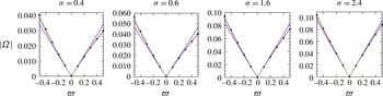
For an ellipsoid in standard position, figure 2 compares the numerically computed rotation rate with the QG approximation as well as the two estimates at next order in Rossby number. Here, we take a horizontal aspect ratio $\unicode[STIX]{x1D6FF}=0.8$ , and four different values of the vertical aspect ratio, $\unicode[STIX]{x1D70E}$ (these are representative). The QG solution has some skill in capturing the rotation rate at lower Rossby numbers ( $|\unicode[STIX]{x1D71B}|<0.2$ ), but, as the PV increases, a noticeable asymmetry appears in the rotation rates for cyclonic and anticyclonic vortices. This departure from the QG solution is well captured by both the analytical solutions for the NQG balance. The only discrepancy occurs for strongly anticyclonic vortices, which are known to be significantly more ageostrophic than their cyclonic counterparts (Tsang & Dritschel Reference Tsang and Dritschel2015). The two analytical solutions themselves are almost indistinguishable, with only slight differences appearing at the highest Rossby number, where the complete analytical solution gives a better estimate than the homogeneous solution in the case of a strongly anticyclonic vortex. The asymmetric behaviour of the cyclonic and anticyclonic rotation rates computed here has also been noted in a previous study by Schecter & Montgomery (Reference Schecter and Montgomery2003). That study also derived analytical solutions for the ageostrophic correction to QG, albeit only for a Rankine (barotropic) vortex surrounded by a skirt of low-lying vorticity.

Figure 2.

Plots of $|\unicode[STIX]{x1D6FA}|$ versus $\unicode[STIX]{x1D71B}$ for an ellipsoid in standard position for four different values of the vertical aspect ratio $\unicode[STIX]{x1D70E}=c/\sqrt{ab}$ , all for a fixed horizontal aspect ratio of $\unicode[STIX]{x1D6FF}=a/b=0.8$ . The thin blue curve is the QG rotation rate $|\unicode[STIX]{x1D6FA}^{(1)}|$ , the thick red curve is the homogeneous balance rotation rate $|\unicode[STIX]{x1D6FA}|=|\unicode[STIX]{x1D6FA}^{(1)}+\unicode[STIX]{x1D6FA}_{H}^{(2)}|$ , the green dashed curve is the complete analytical solution $|\unicode[STIX]{x1D6FA}|=|\unicode[STIX]{x1D6FA}^{(1)}+\unicode[STIX]{x1D6FA}^{(2)}|$ and the black points are the NQG balance values obtained numerically.

4.2.2 Tilted spheroid

We consider next the case of a spheroidal vortex ( $a=b$ ) tilted about the $y$ -axis by an angle $\unicode[STIX]{x1D702}$ with respect to the $z$ -axis (see figure 1 b). Like the case of the ellipsoid in standard position, it has been shown by Miyazaki et al. (Reference Miyazaki, Ueno and Shimonishi1999) that, under the QG approximation, a spheroidal vortex also rotates steadily about the $z$ -axis. For this case we do not solve the full potential problem, but only the homogeneous case where the exterior source terms are set to zero. We start by first considering the general tilted ellipsoid, for which the vortex axis vectors are

(4.34a-c ) $$\begin{eqnarray}\hat{\boldsymbol{a}}=\left(\begin{array}{@{}c@{}}\cos \unicode[STIX]{x1D702}\\ 0\\ -\sin \,\unicode[STIX]{x1D702}\end{array}\right)\!,\quad \hat{\boldsymbol{b}}=\left(\begin{array}{@{}c@{}}0\\ 1\\ 0\end{array}\right)\!,\quad \hat{\boldsymbol{c}}=\left(\begin{array}{@{}c@{}}\sin \unicode[STIX]{x1D702}\\ 0\\ \cos \unicode[STIX]{x1D702}\end{array}\right)\!,\end{eqnarray}$$

and for which the elements of the symmetric matrix $\unicode[STIX]{x1D63D}$ are

(4.35a-c ) $$\begin{eqnarray}\displaystyle & \unicode[STIX]{x1D63D}_{11}=a^{2}+(c^{2}-a^{2})\sin ^{2}\unicode[STIX]{x1D702},\quad \unicode[STIX]{x1D63D}_{22}=b^{2},\quad \unicode[STIX]{x1D63D}_{33}=c^{2}-(c^{2}-a^{2})\sin ^{2}\unicode[STIX]{x1D702},\qquad \quad & \displaystyle\end{eqnarray}$$

(4.35d,e ) $$\begin{eqnarray}\displaystyle & \unicode[STIX]{x1D63D}_{31}=B_{13}=(c^{2}-a^{2})\sin \unicode[STIX]{x1D702}\cos \unicode[STIX]{x1D702},\quad \unicode[STIX]{x1D63D}_{12}=\unicode[STIX]{x1D63D}_{23}=0.\qquad \quad & \displaystyle\end{eqnarray}$$

The leading-order QG solution of Poisson’s equation (3.8) is written in terms of the symmetric matrix $\unicode[STIX]{x1D731}^{1}$ , equation (3.9), and has components

(4.36a-c ) $$\begin{eqnarray}\displaystyle & \displaystyle \unicode[STIX]{x1D731}_{11}^{1}=\unicode[STIX]{x1D709}_{a}+(\unicode[STIX]{x1D709}_{c}-\unicode[STIX]{x1D709}_{a})\sin ^{2}\unicode[STIX]{x1D702},\quad \unicode[STIX]{x1D731}_{22}^{1}=\unicode[STIX]{x1D709}_{a},\quad \unicode[STIX]{x1D731}_{33}^{1}=\unicode[STIX]{x1D709}_{c}-(\unicode[STIX]{x1D709}_{c}-\unicode[STIX]{x1D709}_{a})\sin ^{2}\unicode[STIX]{x1D702},\qquad \quad & \displaystyle\end{eqnarray}$$

(4.36d,e ) $$\begin{eqnarray}\displaystyle & \unicode[STIX]{x1D731}_{31}^{1}=\unicode[STIX]{x1D731}_{13}^{1}=(\unicode[STIX]{x1D709}_{c}-\unicode[STIX]{x1D709}_{a})\sin \unicode[STIX]{x1D702}\cos \unicode[STIX]{x1D702},\quad \unicode[STIX]{x1D731}_{12}^{1}=\unicode[STIX]{x1D731}_{23}^{1}=0.\qquad \quad & \displaystyle\end{eqnarray}$$

The interior source terms needed for the next-order solutions are

(4.37a ) $$\begin{eqnarray}\displaystyle & Q_{\unicode[STIX]{x1D711}}^{2}=2\unicode[STIX]{x1D709}_{a}(\unicode[STIX]{x1D709}_{c}-\unicode[STIX]{x1D709}_{a})\sin \unicode[STIX]{x1D702}\cos \unicode[STIX]{x1D702}, & \displaystyle\end{eqnarray}$$

(4.37b ) $$\begin{eqnarray}\displaystyle & Q_{\unicode[STIX]{x1D713}}^{2}=0, & \displaystyle\end{eqnarray}$$

(4.37c ) $$\begin{eqnarray}\displaystyle & Q_{\unicode[STIX]{x1D719}}^{2}=-2\unicode[STIX]{x1D709}_{c}\unicode[STIX]{x1D709}_{a}+\unicode[STIX]{x1D709}_{a}(\unicode[STIX]{x1D709}_{c}-\unicode[STIX]{x1D709}_{a})\sin ^{2}\unicode[STIX]{x1D702}. & \displaystyle\end{eqnarray}$$

Notably, there is a contribution from both the $\unicode[STIX]{x1D711}^{2}$ and $\unicode[STIX]{x1D719}^{2}$ potentials, while the $\unicode[STIX]{x1D713}^{2}$ potential is zero. This gives rise to the flow matrix

(4.38) $$\begin{eqnarray}\unicode[STIX]{x1D64E}=\left(\begin{array}{@{}ccc@{}}0 & -(\unicode[STIX]{x1D731}_{22}^{1}+\unicode[STIX]{x1D731}_{22}^{2}) & 0\\ \unicode[STIX]{x1D731}_{11}^{1}+\unicode[STIX]{x1D731}_{11}^{2}-\unicode[STIX]{x1D71E}_{31}^{2} & 0 & \unicode[STIX]{x1D731}_{31}^{1}+\unicode[STIX]{x1D731}_{31}^{2}-\unicode[STIX]{x1D71E}_{33}^{2}\\ 0 & \unicode[STIX]{x1D71E}_{22}^{2} & 0\end{array}\right)\!,\end{eqnarray}$$

where the components of the second-order potentials are given by

(4.39a-c ) $$\begin{eqnarray}\displaystyle & \displaystyle \unicode[STIX]{x1D731}_{11}^{2}=\frac{Q_{\unicode[STIX]{x1D719}}^{2}}{\unicode[STIX]{x1D71B}}\unicode[STIX]{x1D731}_{11}^{1},\quad \unicode[STIX]{x1D731}_{22}^{2}=\frac{Q_{\unicode[STIX]{x1D719}}^{2}}{\unicode[STIX]{x1D71B}}\unicode[STIX]{x1D731}_{22}^{1},\quad \unicode[STIX]{x1D731}_{31}^{2}=\frac{Q_{\unicode[STIX]{x1D719}}^{2}}{\unicode[STIX]{x1D71B}}\unicode[STIX]{x1D731}_{31}^{1}, & \displaystyle\end{eqnarray}$$

(4.39d-f ) $$\begin{eqnarray}\displaystyle \unicode[STIX]{x1D71E}_{22}^{2}=\frac{Q_{\unicode[STIX]{x1D711}}^{2}}{\unicode[STIX]{x1D71B}}\unicode[STIX]{x1D731}_{22}^{1},\quad \unicode[STIX]{x1D71E}_{31}^{2}=\frac{Q_{\unicode[STIX]{x1D711}}^{2}}{\unicode[STIX]{x1D71B}}\unicode[STIX]{x1D731}_{31}^{1},\quad \unicode[STIX]{x1D71E}_{33}^{2}=\frac{Q_{\unicode[STIX]{x1D711}}^{2}}{\unicode[STIX]{x1D71B}}\unicode[STIX]{x1D731}_{33}^{1}. & & \displaystyle\end{eqnarray}$$

Considering as in the case of the ellipsoid in standard position that the vortex rotates about the $z$ -axis, we can substitute this flow matrix into (4.29) to solve for the rotation rate about the $z$ -axis. The rotation rate is again the sum of a first- and a second-order term (4.30), where now

(4.40) $$\begin{eqnarray}\unicode[STIX]{x1D6FA}^{(1)}=\frac{a^{2}\unicode[STIX]{x1D709}_{a}-b^{2}\unicode[STIX]{x1D709}_{b}+(c^{2}\unicode[STIX]{x1D709}_{c}-a^{2}\unicode[STIX]{x1D709}_{a})\sin ^{2}\unicode[STIX]{x1D702}}{a^{2}-b^{2}+(c^{2}-a^{2})\sin ^{2}\unicode[STIX]{x1D702}},\end{eqnarray}$$

and, at $O(\unicode[STIX]{x1D716}^{2})$ ,

(4.41) $$\begin{eqnarray}\unicode[STIX]{x1D6FA}_{H}^{(2)}=-\frac{\unicode[STIX]{x1D6FA}^{(1)}}{\unicode[STIX]{x1D71B}}(\unicode[STIX]{x1D709}_{c}(\unicode[STIX]{x1D709}_{a}+\unicode[STIX]{x1D709}_{b})+\unicode[STIX]{x1D709}_{b}(\unicode[STIX]{x1D709}_{a}-\unicode[STIX]{x1D709}_{c})\sin ^{2}\unicode[STIX]{x1D702})-\frac{2\unicode[STIX]{x1D709}_{b}(\unicode[STIX]{x1D709}_{c}-\unicode[STIX]{x1D709}_{a})(c^{2}\unicode[STIX]{x1D709}_{c}-a^{2}\unicode[STIX]{x1D709}_{a})\sin ^{2}\unicode[STIX]{x1D702}\cos ^{2}\unicode[STIX]{x1D702}}{\unicode[STIX]{x1D71B}(a^{2}-b^{2}+(c^{2}-a^{2})\sin ^{2}\unicode[STIX]{x1D702})}.\end{eqnarray}$$

When the tilt angle $\unicode[STIX]{x1D702}=0$ , we recover the solution for the vortex in standard position as in the previous subsection. When the vortex is a tilted spheroid with $a=b$ , we obtain

(4.42) $$\begin{eqnarray}\unicode[STIX]{x1D6FA}^{(1)}=\frac{c^{2}\unicode[STIX]{x1D709}_{c}-a^{2}\unicode[STIX]{x1D709}_{a}}{c^{2}-a^{2}}\end{eqnarray}$$

for the QG solution, showing that the tilted QG spheroid rotation rate is independent of the tilt angle, as was previously derived by Miyazaki et al. (Reference Miyazaki, Ueno and Shimonishi1999). For the NQG correction at $O(\unicode[STIX]{x1D716}^{2})$ , we obtain

(4.43) $$\begin{eqnarray}\unicode[STIX]{x1D6FA}_{H}^{(2)}=-\frac{\unicode[STIX]{x1D6FA}^{(1)}\unicode[STIX]{x1D709}_{a}}{\unicode[STIX]{x1D71B}}[3(\unicode[STIX]{x1D709}_{c}-\unicode[STIX]{x1D709}_{a})\cos ^{2}\unicode[STIX]{x1D702}+\unicode[STIX]{x1D709}_{c}+\unicode[STIX]{x1D709}_{a}],\end{eqnarray}$$

which, unlike the QG case, does depend on the tilt angle of the vortex.

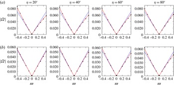
In figure 3 we now show the comparison between the analytical and numerically computed rotation rates for a tilted spheroid. In this case we consider two values of the vertical aspect ratio, $\unicode[STIX]{x1D70E}=0.6$ and $\unicode[STIX]{x1D70E}=1.6$ ( $\unicode[STIX]{x1D6FF}=1$ for a spheroid). For each of these vertical aspect ratios, we consider four values of the tilt angle, 20°, 40°, 60° and 80°. Over the full range of parameters, there is excellent agreement between the analytical and numerical values, both showing the weak variation of the rotation rate with the tilt angle.

Figure 3.

Plots of $|\unicode[STIX]{x1D6FA}|$ versus $\unicode[STIX]{x1D71B}$ for the case of a tilted spheroid ( $\unicode[STIX]{x1D6FF}=1$ ) for four different values of the tilt angles, $\unicode[STIX]{x1D702}$ , and for (a) an oblate vortex, $\unicode[STIX]{x1D70E}=0.6$ , and (b) a prolate vortex, $\unicode[STIX]{x1D70E}=1.6$ . The thin blue curve is the QG rotation rate, $|\unicode[STIX]{x1D6FA}^{(1)}|$ , the thick red curve is the correction using the homogeneous balance rotation rate $|\unicode[STIX]{x1D6FA}^{(1)}+\unicode[STIX]{x1D6FA}_{H}^{(2)}|$ calculated from the analytical formula, and the black points are the numerically computed values obtained from NQG balance.

5 Discussion and conclusions

In this work, we have derived a balanced solution for the motion of an ellipsoidal vortex in a rotating stratified fluid at finite Rossby number. The solution extends the known quasi-geostrophic solution to one higher order in Rossby number, thereby increasing its domain of validity. The solution is obtained from the non-hydrostatic equations by imposing balance (filtering inertia–gravity waves but including ageostrophic effects). This leads to three Poisson equations, having spatially uniform sources within the vortex for an ellipsoid of uniform potential vorticity. The sources outside of the vortex, however, are generally complicated functions of the coordinates. This leads to a difficult matching problem to find the complete analytical solution, which we are able to obtain only for an ellipsoid in standard position (with axes aligned with the coordinate axes). If, on the other hand, we neglect the exterior source terms, we can exploit Laplace’s elegant solution of the problem (Laplace Reference Laplace1784) and write down the closed form analytical solution with a minimum of algebraic effort. This approximation proves to be remarkably accurate in determining the vortex dynamics even for moderate Rossby numbers, as detailed comparisons with computed solutions to the full nonlinear balance model reveal.

In future work, it would be worthwhile investigating the stability of steadily rotating ellipsoids at finite Rossby number. To date, our knowledge of vortex stability has mainly relied on the quasi-geostrophic approximation (Reinaud et al. Reference Reinaud, Dritschel and Koudella2003; Dritschel et al. Reference Dritschel, Scott and Reinaud2005; McKiver & Dritschel Reference McKiver and Dritschel2006), or on full numerical simulations of the non-hydrostatic equations (Tsang & Dritschel Reference Tsang and Dritschel2015). The present work shows that it is possible to accurately describe the undisturbed vortex motion, analytically, to second order in the Rossby number. This may enable a corresponding analytical treatment of stability, helping to shed light on the role played by nonlinear geostrophic effects on, for example, the asymmetry exhibited by cyclonic and anticyclonic vortices. Moreover, it would help quantify the shift in the stability boundary in parameter space as the Rossby number increases, and in particular help identify the vortex characteristics most beneficial for stability (as done in the quasi-geostrophic case by Reinaud et al. (Reference Reinaud, Dritschel and Koudella2003)). Ultimately, the utility of the ellipsoidal model may be judged by comparisons of these stability characteristics with those evidently exhibited by deep, long-lived, isolated three-dimensional mesoscale and sub-mesoscale vortices widely observed in oceanographic surveys (Shapiro & Meschanov Reference Shapiro and Meschanov1991; Paillet et al. Reference Paillet, Le Cann, Carton, Morel and Serpette2002; Ursella, Kovac̆ević & Gac̆ić Reference Ursella, Kovac̆ević and Gac̆ić2011; Bosse et al. Reference Bosse, Testor, Mortier, Prieur, Taillandier, d’Ortenzio and Coppola2015).

Another opportunity to advance this work would be to extend the solutions to multiple vortices, modelled by time-varying ellipsoids, as in the quasi-geostrophic ellipsoidal model (Dritschel, Reinaud & McKiver Reference Dritschel, Reinaud and McKiver2004). This would offer a direct means to comprehensively explore the role of nonlinear ageostrophic effects on vortex interactions, all within a semi-analytical framework.

Most work concerning the ellipsoidal vortex to date has considered the simplest case of uniform PV. In this case, the solutions to the interior Poisson equations have quadratic spatial dependence, subsequently giving rise to a linear velocity field – just what is required to preserve the ellipsoidal form (McKiver & Dritschel Reference McKiver and Dritschel2003). Non-uniform PV was treated by Schecter & Montgomery (Reference Schecter and Montgomery2003), in the special case of a barotropic (two-dimensional) Rankine vortex. They considered a vortex with a central core containing most of the vorticity and an outer region (skirt) of low vorticity decaying weakly away from the centre. They found that the rate of decay of this outer vorticity skirt can affect the stability of the vortex and its ability to resist vertical shear. A similar impact may be expected for three-dimensional, distributed ellipsoidal vortices, but the analysis appears considerably more involved. While there are analytical solutions for ellipsoids with distributed PV in special cases, e.g. for a parabolic interior PV profile matching to uniform PV outside (Chandrasekhar Reference Chandrasekhar1969), the induced velocity has cubic dependence spatially and therefore does not preserve the ellipsoidal form in time. Additional approximations would be required to filter non-ellipsoidal deformations.

While the assumption of uniform PV is idealised, there is support for vortices with sharp edges having nearly discontinuous PV. In two-dimensional flows (with negligible viscosity), the shear or strain felt by a given vortex and induced by surrounding vortices readily strips away low-lying vorticity, leaving a near-discontinuity at the vortex edge (cf. Dritschel Reference Dritschel1998, figure 2, and references therein). The same process is likely to operate in realistic three-dimensional rotating stratified flows, since the essential ingredients are the presence of shear (e.g. surrounding vortices) and negligible viscosity.