1. Introduction
This paper reports the second part of a combined experimental and numerical study aimed at resolving some of the continuing uncertainties over the internal structure and dynamics of the fully developed turbulent mixing layer. As has been discussed in more detail in a companion paper (D’Ovidio & Coats (Reference D’Ovidio and Coats2013) – hereinafter referred to as ‘Part 1’), the classical picture of the mixing layer as a turbulent flow in which the eddying motions are essentially random and three-dimensional was called into question forty years ago when Brown & Roshko (Reference Brown and Roshko1974) observed mixing layers to contain organised processions of quasi-two-dimensional vortex-like large structures at conditions of very high Reynolds number. An identification was immediately made between these structures and the apparently similar vortices produced by excitation of the Kelvin–Helmholtz instability of the free shear flow’s inflected velocity profile. It was already well known that, in mixing layers developing from laminar boundary layers, this instability tends to cause the separated flow to roll up on itself at a naturally preferred frequency to form a regular procession of spanwise-oriented vortices (Michalke Reference Michalke1965). Winant & Browand (Reference Winant and Browand1974) showed that natural excitation of the subharmonics of the fundamental Kelvin–Helmholtz instability can cause the vortices to rotate around each other and amalgamate successively in pairs and proposed this as the mechanism that drives the self-similar growth of the fully developed mixing layer.
This idea that the growth of the fully developed mixing layer is driven by the continued excitation of two-dimensional instability waves has now come to receive very widespread acceptance, although direct evidence that this is actually the operative mechanism has never been provided. Nor has it been satisfactorily explained how the large-scale two-dimensional motions which, in this model, generate the Reynolds stress and entrain irrotational fluid from the free streams feed energy into the continuous cascade of smaller-scale three-dimensional motions. The reader is referred to Brown & Roshko (Reference Brown and Roshko2012) for a recent review of the current state of knowledge on these matters.
The present study has been prompted by the results of some unpublished flow-visualisation experiments carried out by Pedley (Reference Pedley1990) which showed what appeared to be a change in the growth mechanism at the so-called mixing transition. This is the point in the development of the initially laminar flow at which, following the formation of secondary streamwise-oriented vortices on the braids or sheets of strained rotational fluid linking the already existing spanwise vortices (Lin & Corcos Reference Lin and Corcos1984), an amalgamation between two of the latter triggers the establishment of a sustained energy cascade. Up to this point Pedley’s mixing layers grew in thickness by vortex amalgamation in the expected way. After the mixing transition, however, the individual coherent structures all appeared to convect and grow continuously at uniform rates, their spatial growth rate matching and defining that of the layer’s visual thickness. Interactions between the coherent structures still occurred in the post-transition flow but they were quite different in character from their pre-transition counterparts and appeared to occur as a consequence of the growth of the individual structures, not its cause. Some of these interactions were pairings (in the sense that they involved only two neighbouring structures) while others involved three structures and were of the ‘flattening’ or ‘bleeding’ type reported previously by Hernan & Jimenez (Reference Hernan and Jimenez1982). These findings, which in respect of the post-transition flow are completely incompatible with the growth mechanism proposed by Winant and Browand, have been confirmed by the more rigorous and extensive experiments reported in Part 1.
The evidence for this step change in the growth mechanism is at present limited to detailed frame-by-frame analyses of time-resolved but spanwise-integrated flow-visualisation records of the type first produced by Brown and Roshko. Although such records are highly informative, caution is necessary in interpreting purely visual evidence of this kind, especially when the flows concerned are turbulent and contain three-dimensionality. In this paper we present the results of large-eddy simulations (LES) designed to replicate as closely as possible a representative subset of the wind-tunnel experiments reported in Part 1. These simulations confirm in every respect the interpretations placed on the experimental flow visualisations. They also provide information about the three-dimensional aspects of the large-scale organisation and simultaneous spatially and temporally resolved velocity data that are not easily obtainable experimentally.
Numerical simulation has, of course, already been applied very widely in mixing-layer research, most commonly to study the early stages of mixing-layer development from laminar initial conditions. Direct numerical simulations (DNS) have successfully reproduced the initial roll-up to produce the primary spanwise-oriented vortices, the amalgamations of these vortices as a result of the excitation of subharmonics of the fundamental Kelvin–Helmholtz instability, the development of the secondary streamwise-oriented vortices in the braids linking the primary ones and the generation of smaller-scale turbulence by the interaction between the primary and secondary vortices. In the majority of these simulations (e.g. those of Metcalfe et al. Reference Metcalfe, Orzag, Brachet, Menon and Riley1987; Moser & Rogers Reference Moser and Rogers1991, Reference Moser and Rogers1993; Comte, Lesieur & Lamballais Reference Comte, Lesieur and Lamballais1992; Rogers & Moser Reference Rogers and Moser1992) the main focus of interest has been the nonlinear growth and interaction of convective instability modes assumed to propagate with the same constant phase velocity and a temporally evolving shear flow has been taken as a transform of the spatially evolving mixing layer.
In a smaller number of DNS (e.g. those of Buell & Mansour Reference Buell, Mansour, Durst, Friedrich, Launder, Schmidt, Schumann and Whitelaw1989; Wang, Tanahashi & Miyauchi Reference Wang, Tanahashi and Miyauchi2007; Attili & Bisetti Reference Attili and Bisetti2012) separate inflow and exit boundary conditions have been specified, allowing the spatially evolving flow to be simulated directly. Even where dispersion effects are unimportant, spatial simulations with realistic inflow conditions are necessary to replicate the evolution of real mixing layers. This is because (i) the excitation of instability modes in real mixing layers is influenced by feedback from the more fully developed flow further downstream as well as by inflow disturbances, (ii) spatial growth involves asymmetric entrainment from the two free streams and (iii) the development of the mixing layer may be affected by the initial evolution of the inflected free-shear velocity profile in the separated flow.
The spatially evolving DNS of Wang et al. (Reference Wang, Tanahashi and Miyauchi2007) was extended a short distance beyond the mixing transition to study the characteristics of the fine-scale turbulence in the post-transition flow. More recently, Attili & Bisetti (Reference Attili and Bisetti2012) have gone further and performed a high-Reynolds-number spatially evolving DNS to study the statistics of the turbulence where the flow has attained self-similarity. However, direct simulation of the full spectrum of eddies, with its very high computational demands, is not essential if it is the non-isotropic larger-scale motions that are of principal interest. Most attempts to simulate fully turbulent mixing layers have therefore employed LES techniques in which algebraic models are used to represent the finer scales. The additional challenge in LES is the accurate representation of these unresolved scales, and many alternative closure models have been proposed in the literature (Lesieur & Metais Reference Lesieur and Metais1996). Several of these subgrid-scale (SGS) models have been tested comparatively for a mixing layer evolving temporally from laminar initial conditions by Vreman, Guerts & Kuerten (Reference Vreman, Guerts and Kuerten1997).
In many of the researches in which LES has been applied to mixing layers (e.g. those of Jimenez et al. Reference Jimenez, Linan, Rogers and Higuera1997; Comte, Silvestrini & Bégou Reference Comte, Silvestrini and Bégou1998; Balaras, Piomelli & Wallace Reference Balaras, Piomelli and Wallace2001; De Bruin Reference De Bruin2001) it has been applied in parallel with DNS to idealised flows whose parameters have been chosen to facilitate direct comparisons between the results of the two types of simulation. There have been only a few previous studies in which LES has been used to replicate, more or less closely, the measured characteristics of laboratory mixing layers. Zhou & Pereira (Reference Zhou and Pereira2000) and Wang & Milane (Reference Wang and Milane2006) have performed two-dimensional spatial simulations which successfully replicated the entrainment, mixing and chemical reaction in the low-Reynolds-number isothermal reacting mixing layer studied experimentally by Masutani & Bowman (Reference Masutani and Bowman1986), while two-dimensional simulations of fully turbulent laboratory mixing layers have been attempted by Jaberi et al. (Reference Jaberi, Colucci, James, Givi and Pope1999) and Yang et al. (Reference Yang, Zhang, Chan, Lau and Lin2004a ,Reference Yang, Zhang, Chan and Lin b ). Three-dimensional simulations of fully turbulent laboratory mixing layers have been reported by Li, Balaras & Piomelli (Reference Li, Balaras and Piomelli2000), Tenaud et al. (Reference Tenaud, Pellerin, Dulieu and Ta Phuoc2005), Li, Balaras & Wallace (Reference Li, Balaras and Wallace2010) and Biancofiore (Reference Biancofiore2014). In most of these studies the principal motivation for making comparisons with experimental data has been to test aspects of the LES methodology and in no case was any very detailed study made of the evolution of the coherent structures.
The simulations presented here are believed to be the first of any kind to have both replicated fairly closely the laminar initial conditions of particular wind-tunnel experiments and been extended sufficiently far beyond the mixing transition to permit a detailed examination of the large-scale organisation of the post-transition flow. Because the transition is itself dependent on the development of three-dimensional large-scale motions, this has necessarily required spatially evolving simulations in three dimensions. Comparative two- and three-dimensional simulations performed previously by the present authors (McMullan, Gao & Coats Reference McMullan, Gao and Coats2007, Reference McMullan, Gao and Coats2010) have confirmed that, without the three-dimensional large-scale motions, the flow does not undergo the type of transition seen in real mixing layers. It has also required realistic evolution of the inflected velocity profile through the progressive merging of the laminar boundary layers formed on the two sides of the splitter plate. As has been demonstrated elsewhere (McMullan et al. Reference McMullan, Gao and Coats2007, Reference McMullan, Gao and Coats2009), if a symmetrical inflected velocity profile (e.g. one of hyperbolic-tangent form) is taken instead as the inlet condition, not only is the pre-transition development of the flow altered but an unrealistically symmetrical balance of entrainment from the two free streams persists into the post-transition flow.
Although the experiments reported in Part 1 included single- and two-stream mixing layers of low convective Mach number formed between gases of various density ratios, we have restricted ourselves here to four two-stream mixing layers of uniform density with different free-stream velocity ratios. The simulation details will be presented in § 2 and validatory evidence in § 3. These preliminaries will then be followed by the main simulation results in § 4, a brief discussion of their dynamic and kinematic implications in § 5 and a summary of the principal conclusions in § 6.
2. Simulation details
2.1. Code description
The simulations were performed using a well proven LES code in which the mean shear and spatial development were accommodated within two of the three dimensions and the flow was treated as spatially periodic in the third. An implicit filter of top-hat form was used to separate the large energy-carrying scales of motion from the small unresolved scales and a solution was obtained for the continuity and momentum equations
 $$\begin{eqnarray}\displaystyle & \displaystyle \frac{\partial {\bar{u}}_{i}}{\partial x_{i}}=0, & \displaystyle\end{eqnarray}$$
 $$\begin{eqnarray}\displaystyle & \displaystyle \frac{\partial {\bar{u}}_{i}}{\partial t}+\frac{\partial }{\partial x_{j}}{\bar{u}}_{i}{\bar{u}}_{j}=\frac{\partial }{\partial x_{j}}\left[{\it\nu}\left(\frac{\partial {\bar{u}}_{i}}{\partial x_{j}}+\frac{\partial {\bar{u}}_{j}}{\partial x_{i}}\right)+T_{ij}\right]-\frac{1}{{\it\rho}}\frac{\partial \bar{p}}{\partial x_{i}} & \displaystyle\end{eqnarray}$$
 ${\bar{u}}_{i}\ (i=1,2,3)$
and
 $\bar{p}$
are the components of velocity and the pressure associated with the resolved local time-varying motion,
 $$\begin{eqnarray}T_{ij}={\bar{u}}_{i}{\bar{u}}_{j}-\overline{u_{i}u_{j}}\end{eqnarray}$$
is the stress arising from the SGS motions and
 ${\it\nu}$
and
 ${\it\rho}$
are the kinematic viscosity and density of the fluid. If a gradient-diffusion assumption is applied to the SGS motions, the associated stress tensor takes the form
 $$\begin{eqnarray}T_{ij}={\it\nu}_{sg}\left(\frac{\partial {\bar{u}}_{i}}{\partial x_{j}}+\frac{\partial {\bar{u}}_{j}}{\partial x_{i}}\right)+\frac{1}{3}T_{kk}{\it\delta}_{ij}\end{eqnarray}$$
where
 ${\it\nu}_{sg}$
is an eddy viscosity and, if the term containing the Kronecker delta
 ${\it\delta}_{ij}$
is subsumed into the pressure, the momentum equation can be written as
 $$\begin{eqnarray}\frac{\partial {\bar{u}}_{i}}{\partial t}=\frac{\partial }{\partial x_{j}}[2({\it\nu}+{\it\nu}_{sg})\bar{S}_{ij}-{\bar{u}}_{i}{\bar{u}}_{j}]-\frac{1}{{\it\rho}}\frac{\partial \bar{p}}{\partial x_{i}}\end{eqnarray}$$
where
 $$\begin{eqnarray}\overline{S}_{ij}=\frac{1}{2}\left(\frac{\partial {\bar{u}}_{i}}{\partial x_{j}}+\frac{\partial {\bar{u}}_{j}}{\partial x_{i}}\right).\end{eqnarray}$$
To close this system of equations an SGS model is required to evaluate
 ${\it\nu}_{sg}$
. The models used in this study are described in § 2.2.
The code discretised the flow variables on a staggered grid and used second-order central differencing to interpolate between the stored velocities. A multigrid technique was employed to evaluate the pressure term in the momentum equation and time advancement of the solution was effected by the Adams–Bashforth method. A standard convective outflow condition of the form
 $$\begin{eqnarray}\frac{\partial {\bar{u}}_{i}}{\partial t}=-\langle {\bar{u}}_{i}\rangle _{j,k}\frac{\partial {\bar{u}}_{i}}{\partial x_{i}}\end{eqnarray}$$
was applied at the outflow boundary of the computational domain. In this equation
 $\langle {\bar{u}}_{i}\rangle _{j,k}$
represents the resolved outflow velocity, averaged over the whole of the outflow plane.
Transport of a passive conserved scalar
 ${\it\xi}$
within the domain was calculated from the filtered equation
 $$\begin{eqnarray}\frac{\partial \bar{{\it\xi}}}{\partial t}+\frac{\partial }{\partial x_{i}}{\bar{u}}_{i}\bar{{\it\xi}}=\frac{\partial }{\partial x_{i}}\left({\it\alpha}\frac{\partial \bar{{\it\xi}}}{\partial x_{i}}\right)\end{eqnarray}$$
where the diffusivity of the scalar,
 ${\it\alpha}$
, contained a molecular and an SGS component. Because it was only the scalar transport at the resolved scales that was of interest in this study and an eddy-viscosity approach was being taken to the SGS modelling, the latter component was calculated from
 ${\it\nu}_{sg}$
assuming a constant Schmidt number of 0.7. Third-order upwinding was used to calculate the scalar fluxes, the scheme having been chosen to minimise overshoots at the cell boundaries (Gao & Voke Reference Gao and Voke1995). A zero-gradient condition was imposed at the outflow boundary.
2.2. SGS modelling
In this work comparative simulations were carried out using two different SGS models. The first of these was the widely used Smagorinsky (Reference Smagorinsky1963) model in which the assumption of a balance between the rate of energy transfer from the resolved to the unresolved scales of motion and the rate of energy dissipation leads to the formula
 $$\begin{eqnarray}{\it\nu}_{sg}=(C_{S}\overline{{\it\Delta}})^{2}|\overline{S}|\end{eqnarray}$$
where
 $C_{S}$
is an empirical constant,
 $\bar{{\it\Delta}}$
is the filter width and
 $$\begin{eqnarray}|\overline{S}|=(2\overline{S}_{ij}\overline{S}_{ij})^{1/2}.\end{eqnarray}$$
The limitations of this model are well known. The one of greatest concern in the present context is its prediction of a non-zero eddy viscosity in regions of laminar flow. As has been shown in previous work (McMullan et al. Reference McMullan, Gao and Coats2009), this can have the effect of damping the instability modes in the pre-transition part of the mixing layer and delaying the transition itself.
The second model used was the wall-adapting local eddy-viscosity (WALE) model of Nicoud & Ducros (Reference Nicoud and Ducros1999). Here, the eddy viscosity of the unresolved motions is evaluated as
 $$\begin{eqnarray}{\it\nu}_{sg}=(C_{W}\bar{{\it\Delta}})^{2}\frac{(S_{ij}^{d}S_{ij}^{d})^{3/2}}{(\bar{S}_{ij}\bar{S}_{ij})^{5/2}+(S_{ij}^{d}S_{ij}^{d})^{5/4}}\end{eqnarray}$$
where
 $$\begin{eqnarray}\displaystyle & S_{ij}^{d}={\textstyle \frac{1}{2}}({\bar{g}}_{ij}^{2}+{\bar{g}}_{ji}^{2})-{\textstyle \frac{1}{3}}{\it\delta}_{ij}{\bar{g}}_{kk}^{2}, & \displaystyle\end{eqnarray}$$
 $$\begin{eqnarray}\displaystyle & {\bar{g}}_{ij}^{2}={\bar{g}}_{ik}{\bar{g}}_{kj} & \displaystyle\end{eqnarray}$$
 $$\begin{eqnarray}{\bar{g}}_{ij}=\partial {\bar{u}}_{i}/\partial x_{j}.\end{eqnarray}$$
The model constant,
 $C_{W}$
, must again be set empirically, commonly used values ranging from 0.3 to 0.56. This model, developed initially for application to wall-bounded flows, is particularly suitable for the present application because the eddy viscosity vanishes in regions of pure (laminar) shear. It thus overcomes the principal shortcoming of the Smagorinsky model without the high computational cost of a dynamic treatment involving two levels of test filtering.
In earlier work by the present authors (McMullan Reference McMullan2005; McMullan et al. Reference McMullan, Gao and Coats2009) comparisons have also been made with the results of a DNS and of a simulation performed with a ‘structure-function’ SGS model (Metais & Lesieur Reference Metais and Lesieur1992). These comparisons showed no evidence of any significant backscatter from the unresolved to the resolved scales (Piomelli et al. Reference Piomelli, Cabot, Moin and Lee1991) in these three-dimensional spatially evolving mixing layers with the inflow fluctuation levels of interest here.
2.3. Flow conditions
Four of the uniform-density experiments reported in Part 1 were simulated numerically. The inlet free-stream velocities
 $U_{1}$
and
 $U_{2}$
, the value of the velocity parameter
 $$\begin{eqnarray}R=\frac{U_{1}-U_{2}}{U_{1}+U_{2}}\end{eqnarray}$$
and the momentum thicknesses
 ${\it\theta}_{1}$
and
 ${\it\theta}_{2}$
of the boundary layers separating from the two sides of the splitter plate for these test cases are listed in table 1. The experiments F33 and FP42 were carried out with a mixture of helium and argon as stream ‘1’ and air as stream ‘2’, producing a mixing layer of uniform density but non-uniform refractive index which could be visualised by schlieren and shadow techniques. Consequently the kinematic viscosities of the two streams in these experiments differed by approximately 25 %. In the simulations, to avoid the complications introduced by non-homogeneity, both free-stream fluids have been given the viscosity of air and the value taken for
 ${\it\theta}_{1}$
is that measured in the wind tunnel at the same value of
 $U_{1}$
with air instead of the helium–argon mixture as stream ‘1’. Because the Reynolds numbers involved were outside the range in which there is direct viscous damping of the fundamental Kelvin–Helmholtz instability (Ko & Lessen Reference Ko and Lessen1969), any effect of this slight mismatch between the experimental conditions and those created in the simulations is expected to have been very small. The experiments HW9 and HW10 were performed with air in both streams to facilitate hot-wire anemometry and the simulation conditions in these cases match those of the experiments exactly.
Experimental conditions simulated.

The experimental boundary layers were all laminar with shape factors in the range from 2.0 to 2.5, their small departures from Blasius form being a consequence of the fact that the inflows had been accelerated into the test section through nozzles. In the simulations they were given the exact Blasius form with momentum thicknesses equal to the measured values. The inflow plane in the simulations coincided with the trailing edge of the splitter plate and, because the splitter plate in the experiments tapered to a knife edge, it was given zero thickness in the simulations also.
Three-dimensional pseudorandom velocity fluctuations, forming a ‘white noise’ with a uniform intensity of 0.5 % across the frequency range, were superimposed on both inflow streams. This background disturbance environment approximated that present in the experiments in both its intensity level and its broadband character. It may be noted that it was also similar to the inflow condition applied in the most nearly comparable DNS performed to date, that of Attili & Bisetti (Reference Attili and Bisetti2012).
The passive scalar, the transport of which was represented by (2.8), was assigned values of unity and zero at the high- and low-speed inflow boundaries respectively. This scalar was used to provide information about the entrainment into the mixing layer and the fluid mixing, to distinguish rotational from irrotational fluid and also as a means of producing visualisations of the computed flow which could be compared directly with the schlieren visualisations produced in the experiments.
2.4. Computational domain and grid
In the reference experiments the angle of one of the walls of the test section parallel to the splitter plate was adjusted once the flow was established to minimise the mean streamwise pressure gradient. Care was therefore taken to reproduce this condition in the simulations. Approximately uniform free-stream conditions can be achieved in simulations of free shear flows by the use of porous boundaries (Boersma, Brethouwer & Nieuwstadt Reference Boersma, Brethouwer and Nieuwstadt1998), a computational domain with non-parallel boundaries (Ferrero et al.
Reference Ferrero, Kartha, Subbareddy, Candler and Dimotakis2013) or a computational domain with parallel frictionless boundaries located at a distance from the region of shear that is large in relation to the thickness of that region (Attili & Bisetti Reference Attili and Bisetti2012). In this study the last of these approaches was adopted, the domain used replicating the 0.3 m length of the experimental test section in the streamwise (
 $x$
) direction but being given the much larger dimension of 0.61 m in the cross-stream (
 $y$
) direction. This limited the streamwise increase in the value of
 $R$
over the length of the domain to less than 1 % in all cases, a degree of free-stream uniformity greater than was achieved in the experiments. The length of the domain was sufficient to allow full excitation of at least four subharmonics of the fundamental Kelvin–Helmholtz instability.
The domain was divided into 1024 and 240 cells in the streamwise and cross-stream directions. The grid was finest, with spacings of
 ${\rm\Delta}x_{min}=0.00015\ \text{m}$
and
 ${\rm\Delta}y_{min}=0.0004\ \text{m}$
, at the trailing edge of the splitter plate and gradually expanded in both directions. The expansion in the streamwise direction began only after the first 100 cells and had a cell-to-cell scale factor of 1.0014. That in the cross-stream direction had a scale factor of approximately 1.05. This grid geometry ensured that, in every case, the profile of the inflow boundary layer on the high-speed side of the splitter plate and the wavelength of the fundamental Kelvin–Helmholtz mode (excited during the merging of the two boundary layers) were each resolved with more than 20 grid points. It was established that very similar results were obtained with a grid providing half this resolution in these two directions.
To ensure that the results were not affected significantly by the finite extent of the domain in the spanwise (
 $z$
) direction and the periodic boundary condition imposed at the spanwise boundaries both its spanwise extent and the grid spacing in this direction were varied systematically. The domain width
 $L_{z}$
was varied from 0.06 to 0.18 m (the corresponding dimension of the experimental test section was 0.1 m), divided into between 100 and 300 equisized cells.
It should be noted in this context that the simulated flows do not necessarily become fully two-dimensional ‘in the mean’ when considered as a simple time average. This is because in any mixing layer of finite span, whether a physical realisation or a numerical simulation, the spanwise locations of the concentrations of streamwise vorticity tend not to be completely random. For this reason frequent resort will be made in this paper to the spanwise averages of the instantaneous resolved LES output (denoted with angle brackets in the style
 $\langle \,\,\rangle _{z}$
) and to the spanwise averages of the time-averaged single-point values (denoted as
 $\langle \,\,\rangle _{z,t}$
).
The time step in all of the simulations was
 $4\times 10^{-7}\ \text{s}$
. With the grids used this ensured that the Courant–Friedrichs–Lewy number remained below 0.3 at all times. In each simulation 840 000 time steps were computed, outputs being sampled during the final 720 000 steps. This flow duration was sufficient for the whole length of the mixing layer to be swept out by the convecting spanwise-coherent structures some 20 times.
3. Validation
3.1. Validation of the SGS model
The manner and degree to which the simulation results may be affected by the choice of the SGS model and the value given to the constant
 $C_{S}$
or
 $C_{W}$
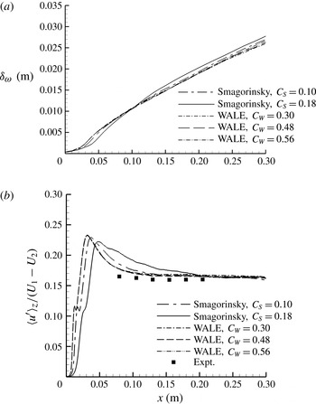
are shown by the comparisons presented in figures 1 and 2. Figure 1(a) shows that with all of the model variations the growth of the mixing layer, as measured by the increase in its spanwise- and time-averaged vorticity thickness
 $$\begin{eqnarray}{\it\delta}_{{\it\omega}}=\frac{U_{1}-U_{2}}{|\partial \langle {\bar{u}}\rangle _{z,t}/\partial y|_{max}},\end{eqnarray}$$
follows the same pattern: the growth rate initially increases slowly as the fundamental Kelvin–Helmholtz instability develops, passes through a maximum as the subharmonics of this instability cause the resultant vortices to amalgamate successively in pairs and then relaxes to a more nearly constant rate in the fully turbulent flow.
Effects of SGS model and model constant on (a) vorticity thickness and (b) r.m.s. of fluctuation of the resolved streamwise velocity, with experimental hot-wire measurements for comparison. Tests performed for case HW9 with
 $L_{z}=0.06\ \text{m}$
,
 ${\rm\Delta}z=0.0006\ \text{m}$
.

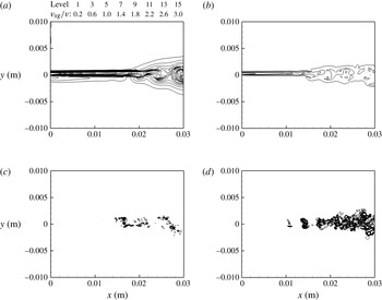
Instantaneous plots of ratio of SGS eddy viscosity to kinematic viscosity at midspan: (a) Smagorinsky model,
 $C_{S}=0.18$
; (b) Smagorinsky model,
 $C_{S}=0.1$
; (c) WALE model,
 $C_{W}=0.3$
; (d) WALE model,
 $C_{W}=0.56$
. Tests performed for case HW9 with
 $L_{z}=0.06\ \text{m}$
,
 ${\rm\Delta}z=0.0006\ \text{m}$
.

These stages in the development of the flow are reflected also in the root mean square (r.m.s.) of the temporal fluctuations in the resolved streamwise velocity,
 $$\begin{eqnarray}u^{\prime }=\sqrt{\langle {\bar{u}}^{2}\rangle _{t}},\end{eqnarray}$$
at the centre of the mixing layer, shown with the experimental hot-wire measurements for comparison in figure 1(b). The contribution of the unresolved fluctuations to the total fluctuation intensity is negligible. The curves plotted to represent the simulation output are again spanwise averages of the single-point r.m.s. values,
 $\langle u^{\prime }\rangle _{z}$
, while the experimental measurements were made at a single midspan location. As is well known from experiments (Spencer & Jones Reference Spencer and Jones1971), the fluctuation intensity at the mixing-layer centreline, scaled on the velocity difference between the free streams, peaks at a little over 20 % in the region in which the vortex amalgamations occur and then relaxes to a lower constant level in the fully turbulent flow.
Figure 1 shows that, with all of the model variations, the growth rate and the turbulence intensity of the fully turbulent layer are exactly the same and that the differences are to be seen only in the developing flow where the Kelvin–Helmholtz instability is still dominant. With the Smagorinsky model and
 $C_{S}=0.18$
(a value known to be too high for use in simulations of wall-bounded flows) the unphysical SGS viscosity created by this model slows the whole development process very considerably. When
 $C_{S}$
is reduced to 0.1 (a slightly more than threefold reduction in the SGS viscosity) this effect on the development length of the flow is reduced roughly in proportion. The WALE model, in contrast, creates no SGS viscosity in regions of pure shear and, in consequence, the development length is insensitive to the value taken for
 $C_{W}$
.
This is further illustrated by figure 2 which shows, for the initial part of the flow, randomly chosen instantaneous plots of the SGS eddy viscosity, normalised by the kinematic viscosity of the fluid, in the midspan plane. With the Smagorinsky model an unphysical eddy viscosity appears at the inflow plane and delays the initial roll-up to an extent that increases with the magnitude of
 $C_{S}$
. With the WALE model a finite eddy viscosity appears only after the initial roll-up has occurred. Although the value of
 $C_{W}$
affects the magnitude of the SGS eddy viscosity beyond this point, this is of no practical importance because, as is shown in figure 1, it has no significant effect on the large energy-containing scales that effect the growth, generate the measured fluctuation intensity and are the subject of this study. In all of the simulations presented below we have used the WALE model with
 $C_{W}=0.56$
.
3.2. Effects of spanwise domain size and grid resolution
It is a matter of concern when apparently two-dimensional large structures appear in a turbulent free shear flow of finite span that this might be a consequence of the spanwise confinement (Biancofiore Reference Biancofiore2014). The extent of the computational domain in this direction,
 $L_{z}$
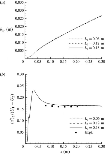
, was therefore varied by a factor of three, with the results shown in figures 3 and 4. As shown in figure 3, the spanwise- and time-averaged growth rates for the three domain widths are almost indistinguishable from each other and so are the plots for the spanwise-averaged resolved fluctuation intensity along the mixing-layer centreline. It can therefore be concluded that the large-scale dynamics of the flow have not been affected significantly by the finite span in any of these three test cases.
Effects of spanwise domain width on (a) vorticity thickness and (b) r.m.s. of fluctuation of the resolved streamwise velocity, with experimental hot-wire measurements for comparison. Tests performed for case HW9 with
 ${\rm\Delta}z=0.0006\ \text{m}$
.

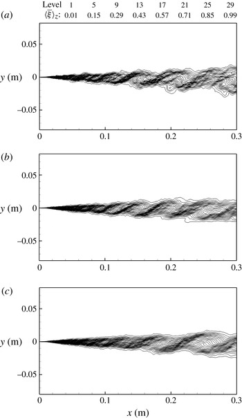
Instantaneous spanwise-averaged contours of the passive scalar for case HW9 with
 ${\rm\Delta}z=0.0006\ \text{m}$
: (a)
 $L_{z}=0.06\ \text{m}$
; (b)
 $L_{z}=0.12\ \text{m}$
; (c)
 $L_{z}=0.18\ \text{m}$
.

Figure 4 shows instantaneous contour plots, chosen at random, of the spanwise-averaged value of the resolved scalar
 $\bar{{\it\xi}}$
. These spanwise-averaged contour plots can be compared directly with the schlieren visualisations presented in Part 1 which similarly make visible the spanwise-averaged scalar gradients within the flow; in both the experiments and the simulations the steep gradients clearly identify the inclined braids which link the spanwise structures. With all three simulation domain widths the same structures are clearly present, the plotted contours merely becoming smoother as
 $L_{z}$
is increased because of the greater spanwise distance over which the averaging is carried out. The impression of two-dimensionality in the spanwise averages therefore increases with
 $L_{z}$
. As will be shown later, these organised structures which form naturally in the developed mixing layer and which undergo the continuous linear growth reported in Part 1 are actually three-dimensional and can be analysed as quasi-two-dimensional spanwise-coherent entities only when examined on a spanwise-averaged basis.
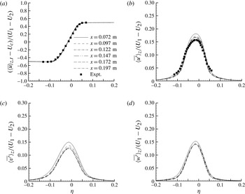
Spanwise-averaged similarity profiles of (a) mean resolved streamwise velocity and r.m.s. of fluctuations of (b) streamwise, (c) cross-stream and (d) spanwise components of resolved velocity for case HW9, with experimental hot-wire measurements for comparison.

Reduction of the grid spacing in the spanwise direction,
 ${\rm\Delta}z$
, from 0.0006 to 0.0004 and 0.0002 m produced results that were indistinguishable from those in figure 3. The definitive simulations were therefore all performed with
 $L_{z}=0.18\ \text{m}$
, divided into 300 equisized cells.
4. Results
4.1. Mean and statistical flow properties
A representative set of profiles of the time- and spanwise-averaged resolved streamwise velocity,
 $\langle {\bar{u}}\rangle _{z,t}$
, and the spanwise-averaged r.m.s. values of the temporal fluctuations of the three components of the resolved velocity,
 $\langle u^{\prime }\rangle _{z},\langle v^{\prime }\rangle _{z},\langle w^{\prime }\rangle _{z}$
, is presented in figure 5. To show the extent to which these computed profiles attain self-similarity
 $\langle {\bar{u}}\rangle _{z,t}$
is related to the reference velocity
 $$\begin{eqnarray}U_{C}=\frac{U_{1}+U_{2}}{2},\end{eqnarray}$$
the velocities are all normalised by the velocity difference between the free streams and the profiles are plotted as functions of the dimensionless coordinate
 $$\begin{eqnarray}{\it\eta}=\frac{y-y_{0}}{x-x_{0}}\end{eqnarray}$$
where (
 $x_{0},y_{0}$
) is the virtual origin of the mixing layer. Similar profiles were obtained for the other three experiments simulated. The profiles for the fluctuations of the filtered velocity in these LES generally resemble those for the fluctuations of the fully resolved velocity in the DNS of Attili & Bisetti (Reference Attili and Bisetti2012) and show the same relaxation to a self-similar state in which the magnitudes of the peaks for the three components scale as
 $u^{\prime }>w^{\prime }>v^{\prime }$
. Also shown for comparison with the computed velocities are the mean and fluctuation profiles measured in the self-similar part of the flow in the corresponding wind-tunnel experiment with a hot-wire anemometer. Because they were made with a single-wire probe, those measurements were of the resultant velocity in the
 $x{-}y$
plane and so, as expected, the experimental fluctuation profile lies between the computed profiles for
 $u^{\prime }$
and
 $v^{\prime }$
.
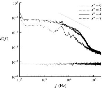
As in the experiments, the computed fluctuation profiles were found to attain self-similarity only downstream of the mixing transition. Although identified originally with reference to the increase in the amount of molecular-scale mixing within the flow (Konrad Reference Konrad1976; Breidenthal Reference Breidenthal1981), this transition is actually that from an unsteady laminar flow to one that is fully turbulent. This is shown by the representative single-point fluctuation spectra presented in figure 6. The transition is characterised statistically by the evolution of the fluctuation energy spectrum at the centre of the mixing layer from one that is dominated by a few large peaks, corresponding to the excited instability modes, to one in which there is a three-dimensional cascade of energy through a range of scales with a roll-off exponent of
 $-5/3$
.
Energy of resolved velocity fluctuations versus frequency at the centre of the mixing layer (case HW9). The reference line indicates the gradient corresponding to a roll-off exponent of
 $-5/3$
.

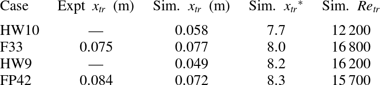
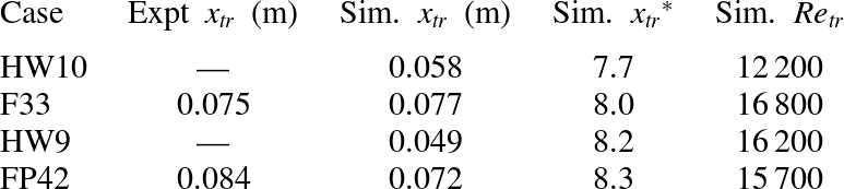
Although spectral analysis gives the impression that the transition is a gradual process, examination of the flow on a time-resolved basis shows that it is actually a step change from unsteady laminar to fully turbulent flow, the location of which moves continuously over considerable distances as the individual triggering vortex amalgamations occur and the resulting turbulent fluid convects downstream. As in the experiments reported in Part 1, the triggering amalgamations were identified individually in the simulation output and their mean location
 $x_{tr}$
for each of the four test cases is listed in table 2 with the corresponding experimental value where available. Also listed are the values at this mean transition location of the ‘pairing parameter’
 $$\begin{eqnarray}x^{\ast }=\frac{0.034Rx}{{\it\theta}_{1}}\end{eqnarray}$$
first proposed by Huang & Ho (Reference Huang and Ho1990) and the Reynolds number
 $\mathit{Re}$
based on the velocity difference
 $U_{1}-U_{2}$
and the mixing-layer thickness
 ${\it\delta}_{vis}$
defined below. The listed values of
 ${x_{tr}}^{\ast }$
are consistent with what was seen in both the experiments and the simulation output – that the transition was typically triggered by the second amalgamation following the initial roll-up. There was considerable cycle-to-cycle variation in the pattern of amalgamation, however, with occasional excursions of the instantaneous transition location to at least twice its mean distance from the splitter plate. This is why the profiles in figure 5 approach self-similarity only well downstream of the mean transition location,
 $x_{tr}$
. The significance of the
 $\mathit{Re}_{tr}$
values is that the Reynolds number must be high enough at the transition location to sustain a continuous energy cascade.
Mean locations of the mixing transition in experiments and simulations.
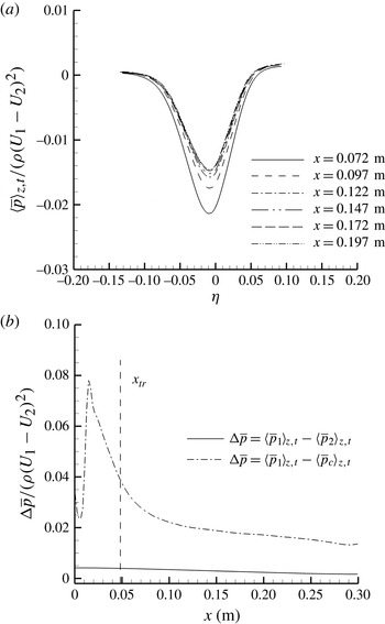
An interesting aspect of the simulation results was that, although there was no significant mean streamwise pressure gradient within the free streams, there were very significant variations in the mean static pressure within the mixing layer. Figure 7(a) plots, for the same test case, some cross-stream profiles of the spanwise average of the time-averaged resolved pressure,
 $\langle \bar{p}\rangle _{z,t}$
, normalised by the density and the square of the inlet velocity difference between the streams. Static-pressure profiles showing a similarly reduced pressure within the region of shear were measured in wind-tunnel experiments carried out by Spencer & Jones (Reference Spencer and Jones1971). They reflect the fact that these organised mixing layers are not classical shear flows but contain regions of low pressure within coherent large vortex structures. Figure 7(b) shows that the mean pressure difference between stream ‘1’ and the centre of the mixing layer,
 $\langle \bar{p}_{1}\rangle _{z,t}-\langle \bar{p}_{C}\rangle _{z,t}$
, reached a peak in the pre-transition flow and, like the velocity profiles in figure 5, relaxed to a more nearly constant level at
 $x\sim 2x_{tr}$
. Figure 7 shows that there is, in this organised mixing layer, also a small pressure difference,
 $\langle \bar{p}_{1}\rangle _{z,t}-\langle \bar{p}_{2}\rangle _{z,t}$
, between the free streams. This latter pressure difference was detected in the experiments reported in Part 1, although its magnitude was too small to be measured accurately.
(a) Cross-stream variation of time- and spanwise-averaged resolved static pressure and (b) its evolution with
 $x$
(case HW9). The two pressure differences plotted in (b) are those between the free streams and between the faster stream and the centre of the mixing layer, with the mean location of the mixing transition shown also for reference.

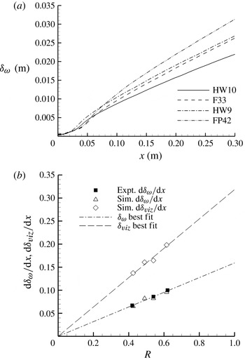
Figure 8(a) shows, for all four test cases, the streamwise growth of the spanwise-averaged vorticity thickness of the mixing layer,
 ${\it\delta}_{{\it\omega}}$
. Consistent with the results already presented, the figure shows all four flows approaching self-similarity downstream of the mean transition location and attaining approximately linear growth at
 $x\sim 2x_{tr}$
. It should be noted that these curves never become perfectly linear, even if a longer domain is used, the growth rate of the mixing layer always continuing to relax slightly towards the exit plane. The same trend is to be seen in other simulations, both of spatially growing plane mixing layers (e.g. those of Li et al.
Reference Li, Balaras and Piomelli2000; Wang et al.
Reference Wang, Tanahashi and Miyauchi2007; Attili & Bisetti Reference Attili and Bisetti2012) and of the mixing layers bounding the potential cores of round jets (Bogey & Bailly Reference Bogey and Bailly2010), in which the flow conditions are comparable with those studied here. This departure from strict self-similarity will be considered further in § 4.3.
(a) Vorticity thickness versus
 $x$
and (b) self-similar growth rates of vorticity and ‘visual’ thickness versus
 $R$
.

Figure 8(b) plots, as a function of
 $R$
for the same four simulations, the spatial growth rate of the vorticity thickness,
 $$\begin{eqnarray}\frac{\text{d}{\it\delta}_{{\it\omega}}}{\text{d}x}=\frac{{\it\delta}_{{\it\omega}}}{x-x_{0}},\end{eqnarray}$$
for the approximately linear part of each curve between
 $x=2x_{tr}$
and the exit plane, together with three corresponding experimental values from figure 3 of Part 1. Because the variation in
 $\text{d}{\it\delta}_{{\it\omega}}/\text{d}x$
over this range of
 $x$
values was no more than 5 % and the limits defining this part of the curve were themselves to some extent arbitrary, a straight average has been taken. Also plotted is a second measure of the growth rate,
 $$\begin{eqnarray}\frac{\text{d}{\it\delta}_{vis}}{\text{d}x}=\frac{y_{0.99}-y_{0.01}}{x-x_{0}},\end{eqnarray}$$
where
 $y_{0.99}$
and
 $y_{0.01}$
are the high- and low-speed edges of the mixing layer as defined by the two rays originating at (
 $x_{0},y_{0}$
) which best fit the 0.99 and 0.01 levels on the profiles of
 $\langle \bar{{\it\xi}}\rangle _{z,t}$
in the same range of
 $x$
values. The mixing-layer thickness defined by these rays is labelled
 ${\it\delta}_{vis}$
because it corresponds approximately to the ‘visual’ thickness measured in flow-visualisation experiments (Brown & Roshko Reference Brown and Roshko1974). As is expected for mixing layers of uniform density,
 ${\it\delta}_{vis}$
is approximately twice
 ${\it\delta}_{{\it\omega}}$
and all of the data support the growth characteristic
 $$\begin{eqnarray}\frac{\text{d}{\it\delta}_{vis}}{\text{d}x}=kR\end{eqnarray}$$
for the post-transition layer with
 $k\approx 0.32$
.
It is well known that, whereas the entrainment of irrotational fluid from the two free streams into the temporally evolving mixing layer is symmetrical, that into the spatially evolving layer is asymmetric and biased in favour of the entrainment from the faster stream. This feature was present in the experiments reported in Part 1 and was captured realistically in these simulations also.
As will be shown in §§ 4.2 and 4.3, the organised post-transition mixing layer is not made up of elements of fluid that convect independently, on average, along near-parallel mean streamlines but of a procession of coherent structures that all occupy the full thickness of the layer and convect bodily in the streamwise direction with the same constant velocity
 $U_{C}$
. In this situation the volumetric entrainment flux of fluid from the faster stream (identified as that for which
 ${\it\xi}=1$
) into unit length and span of the self-similar mixing layer can be evaluated simply as
 $$\begin{eqnarray}\dot{V}_{1}\approx U_{C}\frac{\text{d}{\it\delta}_{vis}}{\text{d}x}\int _{{\it\eta}_{0.01}}^{{\it\eta}_{0.99}}\langle \bar{{\it\xi}}\rangle _{z,t}\text{d}{\it\eta}\end{eqnarray}$$
where
 ${\it\eta}_{0.01}$
and
 ${\it\eta}_{0.99}$
are the points on the profiles at which
 $\langle \bar{{\it\xi}}\rangle _{z,t}$
equals 0.01 and 0.99 respectively. It should be noted that, because the profile being integrated in this case is that of the scalar
 $\langle \bar{{\it\xi}}\rangle _{z,t}$
and not that of the flux
 $\langle {\bar{u}}\bar{{\it\xi}}\rangle _{z,t}$
, the resultant value of
 $\dot{V}_{1}$
is not especially sensitive to the chosen limiting value of
 ${\it\eta}$
on the high-speed side (cf. Brown Reference Brown1974). There is therefore no obvious necessity to distinguish between the rotational and irrotational fluid within the mixing layer in order to evaluate this quantity reliably. The corresponding relation for the fluid entrained from the slower stream (for which
 ${\it\xi}=0$
) is
 $$\begin{eqnarray}\dot{V}_{2}\approx U_{C}\frac{\text{d}{\it\delta}_{vis}}{\text{d}x}\int _{{\it\eta}_{0.01}}^{{\it\eta}_{0.99}}(1-\langle \bar{{\it\xi}}\rangle _{z,t})\text{d}{\it\eta}\end{eqnarray}$$
and so the ratio of the volumetric entrainments from the two streams is
 $$\begin{eqnarray}E_{V}=\frac{\dot{V}_{1}}{\dot{V}_{2}}\approx \frac{\displaystyle \int _{{\it\eta}_{0.01}}^{{\it\eta}_{0.99}}\langle \bar{{\it\xi}}\rangle _{z,t}\text{d}{\it\eta}}{\displaystyle \int _{{\it\eta}_{0.01}}^{{\it\eta}_{0.99}}(1-\langle \bar{{\it\xi}}\rangle _{z,t})\text{d}{\it\eta}}.\end{eqnarray}$$
It is known from experiments (Masutani & Bowman Reference Masutani and Bowman1986) that
 $E_{V}$
is much higher in the unsteady two-dimensional flow upstream of the transition location than in the fully developed flow. To obtain a good approximation to the asymptotic value, therefore, the profiles integrated must be well downstream of the transition region.
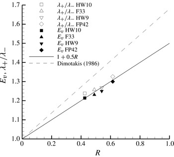
The
 $E_{V}$
values obtained in this way at
 $x=0.2\ \text{m}$
are indicated by the filled symbols in figure 9 and are well fitted by the relationship
 $$\begin{eqnarray}E_{V}=1+0.5R.\end{eqnarray}$$
This is not greatly different from the relation
 $$\begin{eqnarray}E_{V}=1+0.68R\end{eqnarray}$$
proposed by Dimotakis (Reference Dimotakis1986) from consideration of the geometric expansion of scales in the spatially growing mixing layer and measurements made in high-Reynolds-number mixing layers for which
 $R$
was equal to 0.45.
Post-transition entrainment ratio and saddle-point asymmetry versus
 $R$
.

The results presented above show that, in terms of the mean and statistical properties, both the initial development and the post-transition self-similar growth of the experimental mixing layers have been replicated reasonably convincingly in these simulations. Consideration will next be given to the aspects of primary interest in this study – the topography and evolution of the organised large structures in the region downstream of the mixing transition.
4.2. Topography of post-transition structures
Because the large-scale motions in the post-transition mixing layer are inherently three-dimensional, the spanwise coherence within the flow becomes apparent only when the LES output is examined on a spanwise-averaged basis. If the instantaneous field of the resolved scalar
 $\bar{{\it\xi}}$
in a single
 $x{-}y$
plane is considered, there is little clear evidence of any large-scale organisation. However, when the spanwise average is taken, as already seen in figure 4, the bulging of the outer contours around the concentrations of spanwise vorticity and the clustering of the scalar contours to form the inclined braids linking these concentrations of vorticity become very clear. These are, of course, the features shown most clearly in schlieren visualisations which similarly integrate the scalar gradients along the line of sight. Indeed, the resemblance between the flow visualisation provided by these spanwise-averaged contour plots when viewed in animation and the schlieren cine films of the corresponding experimental flows analysed in Part 1 is remarkable. Both show the post-transition flow to comprise a more or less orderly procession of spanwise-coherent structures which occupy the full thickness of the mixing layer and grow continuously as they convect along the layer at a constant velocity. The structures are also seen to undergo occasional interactions which manifest themselves in the disappearance or merging of individual bulges and braids.
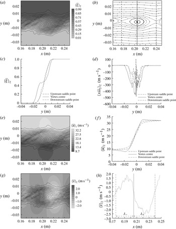
Detailed examination of the spanwise-averaged output for extended periods of flow, each corresponding to the passage of 60 or more of these structures, has shown that the individual structures all possess essentially the same features which they retain throughout most of their lifetimes. These features will be illustrated and discussed with reference to one particular structure, chosen at random at about midlife, from the output for case HW9.
Figure 10(a) shows the spanwise-averaged scalar field centred on the structure with the inclined braids linking this structure to its upstream and downstream neighbours extending to left and right. The outermost contours in the vertical (
 $y{-}z$
) plane through the centre of the structure define the edges of the mixing layer and thus its local visual thickness.
Spanwise-averaged topography of typical post-transition structure (case HW9): (a) field of passive scalar; (b) Lagrangian streamline plot; (c) vertical profiles of passive scalar; (d) vertical profiles of spanwise vorticity; (e) field of streamwise velocity superimposed on contours of passive scalar; (
 $f$
) vertical profiles of streamwise velocity; (g) field of cross-stream velocity superimposed on contours of passive scalar; (h) horizontal profile of cross-stream velocity through centre of core.

That the structure is itself a spanwise-oriented vortex core separated from its neighbours by regions of induced flow is confirmed by the spanwise-averaged streamline plot, figure 10(b), in which the vortex centre and the ‘saddle’ points at which the induced flows stagnate against each other have been reduced to rest by superimposing the velocity
 $-U_{C}$
on the whole field. It is highly significant that the vortex centres in the post-transition mixing layer do not rotate around the saddle points, as happens under the influence of the growing Kelvin–Helmholtz instability waves in the pre-transition flow, but convect at constant velocity along the centreline of the layer. Because the vortices do not themselves undergo any displacements in the cross-stream direction they instead continuously draw tongues of free-stream fluid deep into the mixing layer. It will be shown in § 4.3 that the vortex cores, as visualised by the spanwise-averaged scalar field, all grow continuously at the same constant rate. It is evident, therefore, that the rate of the continuous entrainment into the mixing layer matches the rate at which the entrained fluid is being continuously incorporated into the vortex cores.
A second feature to be noted from figure 10(b) is that the closed streamlines in this spanwise-averaged plot are highly elliptical and occupy only about half of the mixing layer’s visual thickness. This is because the outer half of the core radius in the vertical plane through the core centre is formed by the ends of the braids in which, as will be shown in figure 11, the flow is strongly three-dimensional.


Figure 10(c) shows the profiles of the spanwise-averaged
 $\bar{{\it\xi}}$
in the vertical planes through the vortex centre and the upstream and downstream saddle points. The interesting feature here is the ‘plateau’ in the profile through the centre of the vortex. Like the closed streamlines this plateau occupies approximately half of the core diameter. It becomes flatter when the averaging is carried out over a smaller span and the smoothing effect of the spanwise averaging is reduced. Reference to the corresponding tilting of the contours in (a) shows that the plateau is present only in the vertical cross-section and that, in the horizontal (
 $x{-}z$
) plane through the centre of the core, there is a continuous change in the average fluid composition. The plateau level of
 $\langle \bar{{\it\xi}}\rangle _{z}$
in the vertical profile appears to correspond, at least approximately, to the quantity
 $E_{V}/(E_{V}+1)$
and thus to reflect the relative proportions in which the two fluids are entrained from the free streams. It is presumably this rotation of the average scalar contours in the central part of the core that is responsible for the ‘non-marching’ peak in the probability density function of the fluid composition reported in several experimental studies of post-transition mixing layers (Konrad Reference Konrad1976; Mungal & Dimotakis Reference Mungal and Dimotakis1984; Koochesfahani & Dimotakis Reference Koochesfahani and Dimotakis1986).
The corresponding profiles of the spanwise component of the resolved vorticity,
 $\bar{{\it\omega}}_{z}$
, are shown in figure 10(d). Profiles of this quantity are presented here rather than contour plots because the vorticity in the post-transition mixing layer is relatively diffuse and this, combined with the three-dimensionality of the flow, means that spanwise-averaged contour plots show little of the relevant detail. The vertical profile through the vortex centre shows that most of the spanwise vorticity in this plane is concentrated within the central part of the core (the part corresponding to the closed streamlines in (b) and the plateau in (c)) and falls progressively to zero in the outer parts (formed by the braid ends). As will be shown in figure 11, the braids appear to contain counter-rotating concentrations of streamwise vorticity so that the outer parts of the core in this plane are occupied largely by induced radial currents: radial inflows of irrotational fluid from the free streams alternate, in the spanwise direction, with radial outflows of rotational fluid from the central part of the core. What occurs in these outer parts of the core is thus mainly radial transport with relatively little mixing at the molecular scale. The levels of
 $\langle \bar{{\it\omega}}_{z}\rangle _{z}$
in the profiles through the saddle points are much lower than those in the profile through the vortex centre and it is significant that these profiles show the presence of some positive vorticity (i.e. vorticity of the opposite hand from that of the mean shear). This will be discussed in § 5.
The corresponding field of the resolved streamwise velocity
 ${\bar{u}}$
is shown in figure 10(e) by means of a greyscale superimposed on the scalar contours and the vertical profiles through the vortex centre and the two saddle points are plotted in ( f). The velocity gradient in the plane through the centre of the vortex is seen to be uniform across the central part of the core but to fall away in the parts of the core formed by the ends of the braids, becoming zero close to but within the edges of the mixing layer. This reflects the distribution of
 $\langle \bar{{\it\omega}}_{z}\rangle _{z}$
within the core seen in (d).
As will be discussed in § 5, it is of considerable interest that the induced streamwise accelerations/decelerations within the free streams in this plane through the centre of the vortex are quite localised and small in magnitude. Systematic determinations of the instantaneous maximum and minimum values of
 $\langle {\bar{u}}\rangle _{z}$
in the planes through the centres of all the structures tracked have been made for all of the flow conditions listed in table 1 and the resulting statistics are well fitted by the relationship
 $$\begin{eqnarray}\frac{\langle {\bar{u}}\rangle _{z,max}-\langle {\bar{u}}\rangle _{z,min}}{U_{1}+U_{2}}=1.07R.\end{eqnarray}$$
Thus, any local spanwise-averaged acceleration/deceleration within the free stream on each side of the mixing layer is less than 3–4 % of the velocity difference
 $U_{1}-U_{2}$
. It should further be noted, however, that when these apparent accelerations/decelerations are examined without the spanwise averaging they are found to be non-uniform across the span of the flow and linked to velocity fluctuations of similar magnitude in the other two directions. They thus appear to be associated with the concentrations of streamwise vorticity embedded within the outer parts of each core and a consequence of the fact that, in the regions in which
 $\langle {\bar{u}}\rangle _{z}>U_{1}$
and
 $\langle {\bar{u}}\rangle _{z}<U_{2}$
, the spanwise average of the fluctuation correlation
 $({\bar{u}}-\langle {\bar{u}}\rangle _{z})(\bar{v}-\langle \bar{v}\rangle _{z})$
is non-zero and has a finite negative value. There is no evidence at all in these vertical planes through the vortex centres of the large spanwise-uniform accelerations/decelerations that are induced in the free streams by two-dimensional spanwise-oriented vortices.
To complement figures 10(e) and (f), (g) and (h) show the spanwise-averaged field of the resolved cross-stream velocity
 $\bar{v}$
and the profile of
 $\langle \bar{v}\rangle _{z}$
in the horizontal (
 $x{-}z$
) plane through the centre of the specimen structure. The vertical reference lines in (h) indicate the streamwise locations of the vortex centre and the two saddle points. Taking the velocity extrema in (h) as marking the edges of the core of the vortex in this plane, it can be seen that the core is roughly circular in cross-section at this midlife condition. However, comparison of (h) with ( f) shows that the spanwise-averaged azimuthal velocity at its perimeter is far from constant, being much larger in the vertical plane (where, as was discussed above, its magnitude is very close to
 $(U_{1}-U_{2})/2$
) than in the horizontal one. This is at least partly the effect of the three-dimensional fluctuations across the span of the flow in reducing the magnitudes of the spanwise-averaged velocity extrema,
 $\langle \bar{v}\rangle _{z,max}$
and
 $\langle \bar{v}\rangle _{z,min}$
, in the horizontal plane. This difference between the spanwise-averaged profiles in the two planes is further evidence that, although the core is roughly circular in shape at this midlife condition, the turbulent transport within it is far from axisymmetric.
The fact that the flow field in figure 10(g) is divided so clearly into alternating bands of positive and negative
 $\langle \bar{v}\rangle _{z}$
which extend into the free streams shows that, notwithstanding the radial exchange of rotational and irrotational (free-stream) fluid in the vertical plane through the vortex centre, the entrainment into the mixing layer remains strongly connected to the vortex’s rotation. It is interesting, in this context, to see in (h) that the two saddle points are not equidistant from the vortex centre. Rather, the ratio of the two distances,
 ${\it\lambda}_{+}/{\it\lambda}_{-}$
, correlates, on average, quite closely with the asymmetry of the entrainment from the two streams. This is shown in figure 9 where the averages of the
 ${\it\lambda}_{+}/{\it\lambda}_{-}$
measurements made for all of the tracked structures in all four simulations are plotted on the same axes as the
 $E_{V}$
values discussed in § 4.1.
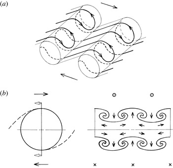
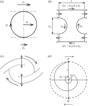
(a) Schematic of secondary vortex lines in the mixing layer (after Bernal & Roshko Reference Bernal and Roshko1986) and (b) cross-section of post-transition coherent structure showing induced radial motions in the outer parts of the core.

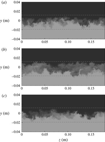
The interpretations placed above on the spanwise-averaged data in figure 10 are consistent with the three-dimensional reconstructions of experimental flow-visualisation data presented by Jimenez, Cogollos & Bernal (Reference Jimenez, Cogollos and Bernal1985). They are also confirmed by figure 11 which shows the scalar field in the
 $y{-}z$
plane at
 $x=0.205\ \text{m}$
at three different times as the same structure convects through this location. The darkest and lightest tones in this figure label the pure (irrotational) fluids entrained from the free streams and the intermediate tones the mixed (rotational) fluid within the core of the spanwise vortex structure and its connecting braids. The horizontal reference lines mark the edges of the mixing layer at the sampling location. In (a) this cross-section cuts through the braid connecting the structure to its downstream neighbour at the centre of the mixing layer in the region of the saddle point. This braid moves downwards towards the lower edge of the layer with the approach of the core and, in (b), the cross-section cuts through the core itself. As the core passes downstream the braid connecting the structure to its upstream neighbour moves downwards from the upper edge of the layer and, in (c), has reached the centre of the layer in the region of the upstream saddle point.
In figures 11(a) and (c) it can be seen that the interface between the two entrained fluids is highly contorted with mushroom-shaped eruptions. These are similar to (but less regular than) the corresponding features in the experimental flow visualisations made just upstream of the mixing transition by Bernal & Roshko (Reference Bernal and Roshko1986) who took them to indicate the presence of a continuous system of counter-rotating streamwise vortex pairs in the braids (figure 12 a). In figure 11(b), where the section cuts through the core of the spanwise structure, the tongues of pure entrained fluid at the two edges of the mixing layer are separated by a thick band of mixed fluid. It has been proposed (Bernal & Roshko Reference Bernal and Roshko1986; Bell & Mehta Reference Bell and Mehta1992) that something similar to the system of streamwise vortices sketched in figure 12(a) survives in the fully turbulent flow, the spanwise spacing of the streamwise vortices increasing in some way to match the increasing spacing of the spanwise structures. A highly idealised representation of the flow in the plane through the core of a spanwise structure might therefore be as sketched in figure 12(b). For simplicity, the cartoons in figure 12 take no account of the spatial growth and represent, in effect, the hypothetical topography of a temporally growing mixing layer. Examination of figure 11(b) shows that, in the simulation of the real spatially growing mixing layer, the tongues of entrained fluid are irregularly spaced and do not all penetrate equally far into the core. In particular, those at the upper edge of the mixing layer tend to be more closely spaced than those at the lower edge. This is consistent with the fact that they form parts of the braids that connect this core to its (smaller) upstream and (larger) downstream neighbours respectively and suggests that the change in the average spanwise length scale is effected continuously in a somewhat random manner.
All of these data show very clearly that the large vortex structures in the post-transition mixing layer are quite different from their substantially two-dimensional counterparts in the pre-transition flow. While they remain as spanwise-coherent concentrations of spanwise vorticity, their cores, as well as being relatively diffuse, are far from axisymmetric and contain strongly three-dimensional features. They are perhaps best thought of as spanwise ‘folds’ in the linking braids, the latter having a thickness of about a quarter of the mixing layer’s visual thickness and containing both spanwise and concentrated streamwise vorticity. Trapped within each fold is a rotating and continuously increasing accumulation of relatively well mixed fluid.
4.3. Large-structure evolution
It was evident from the experimental flow-visualisation data presented in Part 1 that the mechanism by which the mixing layer grew in thickness underwent a step change at the mixing transition. In the pre-transition part of the flow the layer grew as a result of sequential amalgamations between the spanwise-oriented vortices, driven by excitation of the subharmonics of the Kelvin–Helmholtz instability, in the manner proposed by Winant & Browand (Reference Winant and Browand1974). In the post-transition part of the flow there were no further vortex amalgamations of this type, the growth of the layer being associated instead with a continuous linear growth of the individual vortex structures. The same was found in the present simulations.
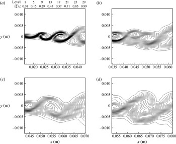
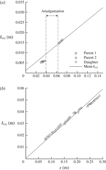
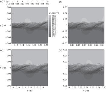
Figure 13 shows the evolution of the spanwise-averaged scalar contours through a representative pre-transition-type vortex amalgamation in the LES output. The particular amalgamation event shown here was one that triggered the transition of the flow to its self-similar fully turbulent state but the amalgamation itself is entirely typical of all the pre-transition pairings that occurred in all of the simulations. Notwithstanding the smoothing effect of the spanwise averaging in this presentation, it can be seen very clearly that the two participating vortices become displaced in the cross-stream direction as they rotate around a common centre and finally amalgamate to form a single larger vortex. Figure 14(a) shows that this process results in a step increase in the visual thickness of the mixing layer (measured, as before, as the cross-stream distance between the outermost contours of
 $\langle \bar{{\it\xi}}\rangle _{z}$
in the planes through the centres of rotation). This growth is the consequence not just of the amalgamation of the rotational cores of the two parent vortices but also of the large entrainment of free-stream fluid into the layer as these vortices gyrate around each other under the influence of the growing Kelvin–Helmholtz instability wave.
Spanwise-averaged contours of the passive scalar at successive times showing a typical pre-transition vortex amalgamation (case FP42).

Streamwise growth of representative individual structures (case FP42): (a) through the pre-transition amalgamation shown in figure 13; (b) in the post-transition part of the mixing layer. The symbols in (b) distinguish individual structures tracked over their lifetimes.

As can be seen in figure 14(a), the vortices in the pre-transition mixing layer grow little between amalgamations. Such continuous growth as they undergo is essentially a consequence of the rapid rotation associated with the highly concentrated vorticity in their cores and the resultant induced stretching of the spiral interface between the two entrained fluids (Jimenez Reference Jimenez1980). In the post-transition mixing layer, in contrast, the rotational cores of the spanwise-coherent turbulent vortex structures described in § 4.2 all grow at a constant rate which matches and defines the self-similar growth of the layer as a whole. This can be seen to be true of the daughter structure produced by the amalgamation that triggered the transition in figure 14(a) and also of the representative selection of post-transition structures whose growth is plotted in figure 14(b). The scatter about the mean growth line of the parallel plots for the individual structures is similar to that in the experimental flow-visualisation data presented in Part 1. It represents a fluctuation in the location of the virtual origin of the self-similar part of the layer and is a consequence of the randomness with which the Kelvin–Helmholtz waves are excited in the pre-transition part of the flow. The continuous linear growth occurs as the individual structures convect in parallel with the free streams at the velocity
 $U_{C}$
without undergoing any displacements in the cross-stream direction. The saddle points convect at the same velocity and maintain the constant separation
 $l={\it\lambda}_{+}+{\it\lambda}_{-}$
, with the centre of the bracketed core positioned a little closer to the upstream than to the downstream saddle point (figure 10
h). As seen in figure 9, the average
 ${\it\lambda}_{+}/{\it\lambda}_{-}$
ratio corresponds, at least approximately, to the ratio of the entrainments from the two streams.
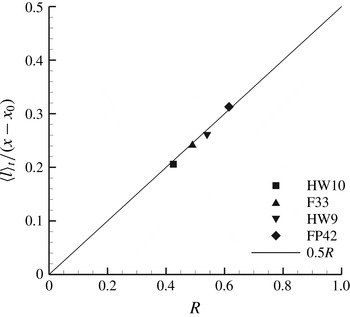
In a mixing layer in which all of the structures are growing continuously these separations cannot be maintained indefinitely, of course. As was seen in the experiments reported in Part 1, so also in the simulations neighbouring structures became involved in interactions with each other at intervals. These reduced the total number of structures in the affected part of the layer and allowed the spacings of the structures that remained to be increased in proportion to the increases that had taken place in their sizes. The resulting progressive increase in the average spacing of the saddle points with the spatial growth is shown in figure 15 where this average spacing
 $\langle l\rangle _{t}$
is plotted, normalised by the distance from the virtual origin, as a function of
 $R$
for all four test cases. The data are well fitted by a straight line of gradient 0.5. This is in reasonably good agreement with the value of
 $0.578R$
obtained by Hernan & Jimenez (Reference Hernan and Jimenez1982) for the normalised mean spacing of the vortex centres in an earlier statistical analysis of an experimental flow-visualisation sequence. (The most probable value in the skewed distribution of their sample was
 $0.51(\pm 0.1)R$
.) Because
 ${\it\delta}_{vis}$
increases like
 $\langle l\rangle _{t}$
in proportion to the distance from the virtual origin, it follows from (4.6) that
 $$\begin{eqnarray}\frac{\langle l\rangle _{t}}{{\it\delta}_{vis}}=\frac{1}{k}\frac{\text{d}(\langle l\rangle _{t}/x)}{\text{d}R}\approx 1.56.\end{eqnarray}$$
Although each core grows in size and entrains from the two free streams at approximately constant rates throughout its life it does not remain circular in cross-section. Figure 16, which can be compared with figure 10(e), shows the spanwise-averaged fields of
 $\bar{{\it\xi}}$
and
 ${\bar{u}}$
at four times in the life of a typical structure. In figure 16(a) this structure is seen immediately after its initial formation in a part of the layer previously occupied by two older structures. At this stage in its life the aspect ratio
 $l/{\it\delta}_{vis}$
of the ‘flow cell’ within which the continuous entrainment and core growth are taking place is substantially greater than the mean value of
 ${\sim}1.56$
. The flow has responded to this situation by stretching the core and tilting it in the anticlockwise direction (evident in the figure from the relative streamwise displacements of the regions of maximum and minimum
 $\langle {\bar{u}}\rangle _{z}$
) to minimise the stretching of the braids and the effect of the high aspect ratio on the entrainment from the free streams. In (b) and (c) the aspect ratio is closer to the mean value, the core is more nearly circular in cross-section and the two braids become tangential to the core in the same vertical plane. In (d) the aspect ratio is substantially smaller than the mean value, the core has become stretched again and is now tilted in the clockwise direction, again minimising the effect of the altered cell geometry on the braid length and the entrainment from the free streams.
Normalised mean saddle-point spacing in the post-transition mixing layer versus
 $R$
.

Spanwise-averaged field of the streamwise velocity superimposed on the contours of the passive scalar showing the evolution through the lifetime of a typical post-transition structure (case HW9).

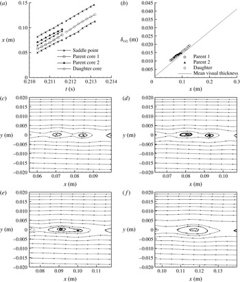
As in the experiments reported in Part 1, the interactions that ended the lives of the individual structures in the simulations were of two basic types. The more common involved just two neighbouring structures but, unlike the pre-transition pairings, was completed without either of them undergoing any displacement in the cross-stream direction. The centres of rotation and saddle points associated with the participating structures are tracked through a typical interaction of this type in figure 17(a). In effect the two parent structures are replaced by a single new structure whose centre of rotation is located between those of its parents. In the experimental schlieren and shadowgraph visualisations it appeared that both parent structures broke down completely in the course of this type of interaction. However, examination of the spanwise-averaged streamlines provided by the simulations (figure 17 c–f) shows that it is actually the central part of the core of the upstream parent that forms the nucleus of the new structure, being itself displaced downstream to fill the gap in the procession of structures left by the destruction of its partner.
(a) Convection of core centres and saddle points, (b) growth of cores and (c–f) evolution of spanwise-averaged streamlines through a typical post-transition pairing interaction (case HW10).

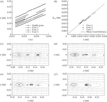
The other type of interaction, illustrated by figure 18, occurred when a structure became closely confined by both of its immediate neighbours simultaneously. In these circumstances the trapped core ceased to entrain, became stretched and tilted in the clockwise direction and either collapsed with its linking braids to form a single new braid linking its neighbours or, as in the example illustrated, was torn in two and consumed by them. In all of these triple interactions (which can be identified with the ‘flattening’, ‘bleeding’, ‘tearing’ and ‘sacrificial’ interactions described by Damms & Küchemann (Reference Damms and Küchemann1974), Hernan & Jimenez (Reference Hernan and Jimenez1982) and Pedley (Reference Pedley1990)), the neighbouring cores continued their own steady convection and growth without interruption.
(a) Convection of core centres and saddle points, (b) growth of cores and (c–f) evolution of spanwise-averaged streamlines through a post-transition ‘tearing’ interaction (case HW10).

It is evident that both types of post-transition interaction occur as a consequence of the continuous linear growth undergone by the individual structures and function merely to remove at intervals structures that can no longer be accommodated within the available flow length. It was suggested in § 4.2 that the spanwise-coherent structures in the post-transition flow are best regarded as folds in the braids. Viewed in that light the large-structure interactions simply smooth out individual folds so that, on average, the proportions defined by (4.13) are maintained as the thickness of the braids and the scale of the folding increase.
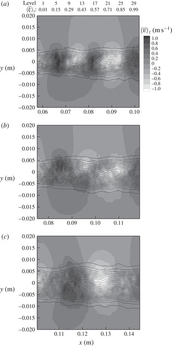
It is important to note that the entrainment of free-stream fluid and mixing-layer growth continue without interruption at essentially the same constant rates through both types of post-transition interaction. Figure 19 shows the evolution of the field of
 $\langle \bar{v}\rangle _{z}$
through the pairing interaction tracked in figure 17. As in the similar figure 10(g) considered earlier, the presence of the spanwise-coherent entraining structures is indicated by the alternating vertical bands of positive and negative velocity extending across the full thickness of the mixing layer and into the free streams. In figure 18(a) the centres of the interacting structures are located at
 $x\sim 0.07$
and
 ${\sim}0.85\ \text{m}$
and a saddle point exists between them at
 $x\sim 0.079\ \text{m}$
. Throughout the course of the interaction the cross-flows continue without interruption on the sides of the interacting structures remote from this saddle point. The entrainment into the mixing layer also continues in the interaction region itself but, as the interaction develops (figure 19
b), the bands of positive and negative
 $\langle \bar{v}\rangle _{z}$
first contract so that they do not extend beyond the centreline of the layer and then merge with the adjoining bands (figure 19
c). The continuance of the same rate of mixing-layer growth through the interaction is seen in figure 17(b) which plots the growths of the cores of the two interacting structures and of the new core that emerges from the interaction. It shows the new core resuming, a little further downstream, the same linear growth characteristic that had been followed by its parents, the entrainment into the mixing layer having continued at essentially the same rate throughout the period in which the redistribution of vorticity was taking place.
Evolution of the spanwise-averaged cross-stream velocity field and passive-scalar contours through the post-transition pairing interaction tracked in figure 17.

These data show that there is, in the post-transition mixing layer in its organised state, a strong natural preference for the maintenance of particular rates of entrainment from the two streams which contributes to the self-preserving character of the large-scale organisation. In particular, figure 19 shows the way in which the maintenance of these preferred rates of entrainment by the organised flows in the adjacent cells conditions to a large degree the course and outcome of a localised breakdown in the large-scale organisation. There is thus, at every streamwise location in the post-transition layer, a large-scale influence of the spatial growth occurring further up- and downstream. In numerical simulations the influence of the self-similar growth further downstream is progressively removed towards the downstream end of the computational domain and it is thought to be this that is responsible for the slight departures from perfect self-similarity in the data presented in figures 5, 7 and 8.
5. Discussion
5.1. Dynamics of the post-transition mixing layer
The simulation results presented in § 4 are fully consistent with the results of the flow-visualisation experiments reported in Part 1 and provide confirmatory evidence that what was seen in those experiments (and also in the earlier unpublished experiments of Pedley (Reference Pedley1990)) was not an artefact of either wind-tunnel peculiarities or the flow-visualisation techniques employed. Both approaches show that the fully turbulent self-similar mixing layer remains naturally organised on the scale of the local layer thickness for some distance at least beyond the mixing transition. Contrary to what has been generally assumed until now, however, they also show that the post-transition coherent structures do not grow by amalgamation in the manner of their pre-transition counterparts but individually undergo continuous linear growth. This seems to rule out the suggestion first put forward by Winant & Browand (Reference Winant and Browand1974) that the growth of turbulent mixing layers in their fully developed state is driven by the continued excitation of Kelvin–Helmholtz instability waves. As was discussed in Part 1, the linear character of the continuous growth undergone by the post-transition structures also seems to rule out any explanation of this continuous growth in terms of either two-dimensional passive induction (Jimenez Reference Jimenez1980) or two-dimensional turbulent diffusion (Moore & Saffman Reference Moore and Saffman1975).
What has been made clearer by the present simulations is that the dynamics of the mixing-layer growth become intrinsically three-dimensional at the mixing transition. If numerical simulations are performed in two dimensions no transition of the type that was seen in the experiments occurs and subharmonics of the fundamental Kelvin–Helmholtz mode continue to be excited naturally throughout the available flow length (McMullan et al. Reference McMullan, Gao and Coats2007, Reference McMullan, Gao and Coats2010). If the simulations are performed in three dimensions, on the other hand, the secondary streamwise vortices are able to develop and interact with the primary spanwise vortices to produce the transition at which point, as was shown in § 4.3, there is a switch to the regime in which the large structures all undergo continuous linear growth. Three-dimensionality is, of course, already present in the pre-transition flow in the form of the secondary instability which leads to the formation of the streamwise vortices. At this stage in the development of the flow, however, its presence has little or no effect on the growth of the two-dimensional Kelvin–Helmholtz modes. The critical change that occurs at the mixing transition is that the spanwise vortices become the largest in a continuous three-dimensional cascade of eddying motions and energy is no longer able to accumulate in two-dimensional instability modes of lower frequency.
It should be noted that, in the context of the post-transition mixing layer, three-dimensionality involves more than the enhanced diffusion resulting from the presence of small-scale three-dimensional motions. All that an ‘eddy viscosity’ can do in an otherwise two-dimensional shear flow is diffuse spanwise vorticity of constant circulation. The other effect of three-dimensionality is to introduce an additional degree of freedom into the evolution of the flow. The streamwise vortices, the presence of which can be inferred from
 $y{-}z$
scalar plots such as those in figure 11, create with the large spanwise vortices a three-dimensional matrix of vortex lines that can be stretched and bent in complex ways, allowing the original spanwise-oriented vorticity to become intensified locally, reoriented in the streamwise and cross-stream directions or even reversed in sign. The presence of positive spanwise vorticity in the computed flow field (see figure 10
d) provides direct evidence that these vortex stretching and bending effects are significant, as does the
 $-5/3$
roll-off exponent of the energy cascade to smaller scales (figure 6). It follows that the widely discussed concept of ‘two-dimensional turbulence’, in which enstrophy considerations require an inverse energy cascade to larger scales of motion (Kraichnan Reference Kraichnan1967), while possibly applicable to the pre-transition flow, has no relevance to the post-transition pattern of growth we seek to understand here.
If the Winant & Browand (Reference Winant and Browand1974) mechanism is not active beyond the mixing transition then it must be asked why it is that the post-transition mixing layer continues to be organised in a manner superficially similar to that of the pre-transition flow. As was seen in § 4.2, although there is both large- and small-scale three-dimensionality in the post-transition mixing layer, when the flow is examined on a spanwise-averaged basis, it is still found to consist of concentrations of spanwise vorticity separated by regions of induced flow. The answer must simply be that this type of large-scale organisation minimises the resistance to the applied shear.
The general dynamic principle governing the evolution of any macroscopic non-equilibrium system with time-invariant boundary conditions (in the absence of any periodic forcing this includes the mixing layer) is that the system will progressively approach its final equilibrium state by the path that minimises its internal rate of entropy production (Glansdorff & Prigogine Reference Glansdorff and Prigogine1964). This is why, at a very early stage in its development, the separated laminar shear flow becomes unstable and repeatedly reorganises itself into configurations in which the vorticity shed from the splitter plate is concentrated within a diminishing number of vortex cores; with each reorganisation a situation is created transiently in which there is potential flow external to the vortex cores and the rate of entropy production by viscous action is minimised. It must be supposed that the fully turbulent mixing layer adopts the organised three-dimensional configuration seen in these simulations, where circumstances allow, because this involves a lower rate of entropy production than in the corresponding completely random turbulent shear flow.
That the large-scale organisation of the post-transition flow does in fact provide a low-entropy-production path by which the non-equilibrium situation created by the applied shear can be progressively relaxed is deducible from the simulation output. It was shown in § 4.2 that the spanwise structures are not two-dimensional vortices and that interposed between the free streams and the central parts of their cores are the thick zones of three-dimensional motion formed by the braid ends (figure 12
b). It was further shown (figure 10
f) that, considered on a spanwise-averaged basis, any streamwise-velocity fluctuations induced in the free streams in the
 $y{-}z$
plane through the centre of each structure are very small in amplitude. An analogy can therefore be made between each structure and an imagined solid roller being rolled frictionlessly between the free streams with the azimuthal velocity
 $$\begin{eqnarray}U_{{\it\theta}}\approx \frac{U_{1}-U_{2}}{2}\end{eqnarray}$$
at its perimeter (figure 20
a). The analogy is not an exact one because the motions in the outer parts of the flow structure are strongly three-dimensional and the perimeter of the structure is not precisely defined. However, (4.12) indicates that any error in the effective value of
 $U_{{\it\theta}}$
given by (5.1) cannot be greater than 7 % and, as was argued in § 4.2, the apparent difference between the two equations is at least partly a nonlinear effect of the three-dimensional motions on the spanwise average of
 ${\bar{u}}$
.
(a) Idealised ‘roller’ motion of the post-transition coherent structure. (b) Geometry providing potential flow within the organised post-transition mixing layer. (c) Entrainment into the organised post-transition mixing layer by induced radial exchange in the vertical plane through the centre of the structure and as part of the saddle flow pattern. (d) Equiangular spiral defining the temporal growth of the post-transition coherent structure.

Consider now the flow in the parts of the mixing layer external to the rotational cores of the large structures. It was shown earlier (4.13) that the average spacing of the structures is 1.56 times the local visual thickness. Drawn to scale, considered as a spanwise average and viewed in the Lagrangian frame in which the cores have been reduced to rest, the part of the mixing layer between two adjacent cores can therefore be represented as shown in figure 20(b). The significance of this spacing is that, with
 $$\begin{eqnarray}\frac{l}{{\it\delta}_{vis}}=1.56\approx \frac{{\rm\pi}}{2},\end{eqnarray}$$
the net circulation within the circuit ABCDEFGHA embracing all of the fluid external to the cores and extending an arbitrary distance into the free streams is zero, implying potential flow within this circuit. In this midlife situation for the pair of neighbouring cores represented there is no stress tangential to the lines DE and HA and therefore no entropy production within this length of the mixing layer as a direct result of the applied mean shear. The figure shows, for simplicity, the two cores as having equal diameters but the argument is not affected in any way if they are given different diameters to take account of spatial growth and the average of their diameters is used in (5.2).
It thus appears that, by organising itself in this way, the three-dimensional post-transition mixing layer is able to achieve a situation analogous to the one that exists transiently as each excited Kelvin–Helmholtz mode attains saturation in the two-dimensional flow. As soon as a Kelvin–Helmholtz instability has saturated, however, the vortex produced by that instability begins to decay and its vorticity becomes dispersed again. The evidence of figure 14(b) and the corresponding experimental data presented in Part 1 is that the three-dimensional mass, momentum and energy transport in the post-transition mixing layer are such that the circulation of each core (
 $={\rm\pi}{\it\delta}_{vis}U_{{\it\theta}}$
if the roller-bearing analogy is retained) is able to increase linearly throughout its lifetime. This would be impossible in a two-dimensional mixing layer because the total circulation of the spanwise vorticity in the length
 $l$
of the mixing layer is
 $l(U_{1}-U_{2})$
and, once the core had attained a diameter of
 $2l/{\rm\pi}$
, it would already have swept up all of the vorticity available. As was discussed above, in the three-dimensional mixing layer this limitation does not apply because additional spanwise vorticity can be produced by the stretching and bending of vortex lines if this is balanced by an equal production of spanwise vorticity of the opposite hand.
Because the self-similar growth of the organised post-transition mixing layer is both defined and effected by the continuous linear growth of the individual structures, the entrainment into the mixing layer must be understood as continuous and as an integral aspect of the process by which the structures grow. It was shown in figure 9 that the bias of the entrainment in favour of that from the faster stream correlates very closely with the ratio of the average distances from the centre of each structure to the downstream and upstream saddle points. This links the entrainment bias in a very obvious way to the relative sizes of the tongues of irrotational fluid drawn deep into the mixing layer on the downstream and upstream sides of each structure. This quasi-two-dimensional contribution to the entrainment is clearly the consequence of the fact that the spanwise vorticity is concentrated within the cores of the structures but it is continuous, not linked to instability-driven vortex amalgamations as in the pre-transition flow. Much of the fluid continuously drawn into the mixing layer in this way subsequently becomes incorporated into the rotational cores of the structures as a consequence of their continuous growth.
However, this is not the whole of the entrainment into the mixing layer. In the
 $y{-}z$
planes through the centres of the structures there is a direct exchange of free-stream fluid and the rotational core fluid as a result of the radial transport induced by the counter-rotating concentrations of streamwise vorticity in the braid ends (figure 20
c). From the spanwise-averaged viewpoint this radial exchange can be considered as turbulent diffusion, free-stream fluid being, in effect, peeled away continuously from the free streams and becoming attached to the cores of the rotating structures with little or no change in its streamwise velocity. Its rate must be a function of the strengths and spacings of the concentrations of streamwise vorticity, however, not an eddy viscosity scaled directly on the mixing-layer thickness. If, as seems likely, the strength:spacing ratio of these concentrations of streamwise vorticity remains constant the cores can be expected to ‘nibble’ away at the free streams in this plane through the core centre at the observed constant rate. If the radial exchange were instead driven by a more generalised eddy viscosity the core diameter would grow as the square root of time (Moore & Saffman Reference Moore and Saffman1975). The entrainment into the post-transition mixing layer thus seems to occur by a balanced combination of the continuous large-scale ‘engulfment’ induced by the co-rotating concentrations of spanwise vorticity and continuous ‘nibbling’ by the counter-rotating concentrations of streamwise vorticity in the braid ends.
5.2. Kinematics of mixing-layer growth
According to classical turbulence theory, the rate of growth of a turbulent shear flow is indeterminate and must be evaluated empirically. In the special case of the organised post-transition mixing layer, however, it follows from the descriptions of the flow organisation given above that the rates of the continuous entrainment and growth are actually determined kinematically.
As was discussed above, the computed spanwise-averaged profiles of
 $\bar{{\it\xi}}$
,
 $\bar{{\it\omega}}_{z}$
and
 ${\bar{u}}$
in the vertical plane through the centre of each large vortex structure show (figures 10
c,d,f and 14
b) that, in this plane, the core of the structure grows continuously at a constant rate while rotating about its centre with a constant azimuthal velocity
 $U_{{\it\theta}}$
at its perimeter. In this plane through the core centre irrotational fluid is, in effect, being peeled continuously away from the free streams and wound onto the growing core at a constant rate. If the fluid is incompressible, kinematics require that the radius of the core in this plane,
 $r\ (={\it\delta}_{vis}/2)$
, will increase by the factor
 $e$
for each complete revolution and that the locus in polar coordinates of the point
 $P$
on the perimeter of the core will be an equiangular spiral of the form
 $$\begin{eqnarray}\frac{r}{r_{0}}=\exp \left(\frac{|{\it\theta}-{\it\theta}_{0}|}{2{\rm\pi}}\right)\end{eqnarray}$$
(figure 20
d), where
 $r_{0}$
and
 ${\it\theta}_{0}$
are some finite initial radius and angle of rotation. The locus of the point
 $Q$
will be the mirror image of the locus of
 $P$
. It is important to note that we are considering here only the loci of these two points in the vertical plane through the core centre and that the broken circle drawn in the figure is a purely geometrical construction; we are not assuming that the core is actually circular in cross-section, that fluid attaches itself to the core at the same rate around the whole of its perimeter or that the azimuthal velocity is constant around the perimeter of the core. This analysis is therefore not dependent in any way on the heuristic roller-bearing analogy invoked in § 5.1; it follows directly from the self-similar evolution of the profiles of
 $\langle \bar{{\it\xi}}\rangle _{z}$
,
 $\langle \bar{{\it\omega}}_{z}\rangle _{z}$
and
 $\langle {\bar{u}}\rangle _{z}$
seen in the simulations.
Now, differentiation of (5.3) gives
 $$\begin{eqnarray}\frac{\text{d}r}{\text{d}t}=\frac{\text{d}r}{\text{d}{\it\theta}}\frac{\text{d}{\it\theta}}{\text{d}t}=\frac{r_{0}}{2{\rm\pi}}\exp \left(\frac{|{\it\theta}-{\it\theta}_{0}|}{2{\rm\pi}}\right)\frac{U_{{\it\theta}}}{r}=\frac{U_{{\it\theta}}}{2{\rm\pi}}.\end{eqnarray}$$
However, from (2.15), (4.1) and (4.6) the temporal rate of growth of the diameter of each core is
 $$\begin{eqnarray}\frac{\text{d}{\it\delta}_{vis}}{\text{d}t}=\frac{\text{d}{\it\delta}_{vis}}{\text{d}x}\frac{\text{d}x}{\text{d}t}=kRU_{C}=k\frac{U_{1}-U_{2}}{2}.\end{eqnarray}$$
If
 $U_{{\it\theta}}$
is related to the free-stream velocities by (5.1) it follows, from the combination of these relationships, that
 $$\begin{eqnarray}k=\frac{1}{{\rm\pi}}\approx 0.32.\end{eqnarray}$$
This is the same value as best fits the data in figure 8(b). It lies at the lower end of the range of values commonly measured in wind-tunnel experiments but this is as expected because it applies specifically to the post-transition mixing layer in its organised state. As was shown in Part 1, the temporary breakdowns in the large-scale organisation that commonly occur in real mixing layers are accompanied by a displacement of the mixing-layer centreline towards the faster stream. This intermittent displacement of the mixing layer in the cross-stream direction has the effect of broadening the mean velocity and scalar profiles as measured with conventional traversing techniques with a consequent increase in the measured value of
 $k$
.
The spiral defined by (5.3) is simply a geometric transform which imposes the requirement for continuity on the self-similar growth of the individual large structures and thus on the self-similar growth of the post-transition mixing layer as a whole. It should not be confused with the spiral formed by the rolling up of an infinite vortex sheet – a construction that has been taken to define the growth rate in some two-dimensional analyses of turbulent mixing layers (Jimenez Reference Jimenez1980; Goldshtik & Hussain Reference Goldshtik and Hussain1995). The implication of the present analysis is that the organised turbulent mixing layer grows at a rate very close to that defined by (5.6) because that is the only growth rate at which the requirement for continuity allows the flow to minimise its rate of entropy production in the manner discussed in § 5.1. The necessary balances of mass, momentum and energy have, of course, all been computed rigorously within the simulations. It can therefore be further concluded that the inherent three-dimensionality of the flow and the presence of the continuous cascade of eddy scales together provide the flexibility needed for the growth to be sustained at this unique rate while satisfying also the necessary balances of momentum and energy.
6. Conclusions
-
(i) Large-eddy simulations of homogeneous mixing layers developing spatially from laminar boundary layers have been performed for different free-stream velocity ratios, replicating four of the wind-tunnel experiments reported in Part 1. The simulations were continued through the mixing transition and into the fully turbulent self-similar flow beyond.
-
(ii) When the three-dimensional LES output was analysed on a spanwise-averaged basis the post-transition mixing layer was found to be occupied by an almost continuous procession of spanwise-coherent vortex-like large structures. As appeared to be the case in the experiments, the familiar mechanism of growth by vortex amalgamation was replaced at the mixing transition by one in which the large structures individually underwent continuous linear growth. The interactions between neighbouring structures that occurred in the post-transition flow were a consequence of this continuous growth and functioned simply to reduce the number of structures at intervals so that a constant average spacing-to-thickness ratio was maintained and the growth of those that remained could continue unimpeded. These post-transition interactions were different in character from their pre-transition counterparts.
-
(iii) Detailed examination of the spanwise-averaged LES output has shown that the post-transition large structures are turbulent vortex cores which occupy the whole thickness of the mixing layer and convect in the streamwise direction at a velocity very close to the average of the free-stream velocities without themselves undergoing any displacements in the cross-stream direction. It has also shown that the post-transition structures do not induce significant streamwise accelerations/decelerations within the free streams but are rolled in an essentially passive manner between them. The continuous linear growth of the structures is matched by continuous entrainment from the free streams, the inflows of irrotational fluid producing stable regions of near-potential flow in the spaces between the rotational structures. The bias in favour of entrainment from the faster stream is a little smaller than that suggested in the model of Dimotakis (Reference Dimotakis1986).
-
(iv) The kinematics of the continuous linear growth of the large structures define a temporal growth rate that determines also the spatial growth rates of homogeneous mixing layers in this organised post-transition state. The constant relating the temporal growth rate of the visual thickness to the velocity difference between the free streams has a value equal to or very close to
 $(2{\rm\pi})^{-1}$
.
-
(v) The simulations have shown that an essential role in the post-transition mechanism of continuous entrainment and growth is played by streamwise vorticity contained within the braids. Concentrations of this streamwise vorticity appear to be responsible for the radial exchange of rotational and free-stream fluid in the outer parts of the spanwise structures and for the necessary three-dimensional redistribution of the vorticity within the mixing layer. The continuous interaction between the concentrations of streamwise and spanwise vorticity can also be seen as providing the mechanism by which a proportion of the energy associated with the mean shearing motion is fed continuously into the cascade of smaller-scale eddying motions.

Acknowledgements
The simulations presented here were performed using ALICE, the University of Leicester High Performance Computing Facility.
The authors wish to record that the relevance of the logarithmic spiral to a mixing-layer model in which the large structures grew continuously at a constant rate was first suggested in unpublished work carried out by the late J. P. D. Hakluytt during the years 1975–1985 at the UK’s National Gas Turbine Establishment. This paper is dedicated to his memory.