



1. Introduction
Resonant wave interactions have been studied extensively for surface waves on a homogeneous layer as a main mechanism to determine the spectral distribution of wave energy (Hammack & Henderson Reference Hammack and Henderson1993; Janssen Reference Janssen2004). It is well known that the primary resonant interactions occur among four waves at the third order of nonlinearity for surface gravity waves (Phillips Reference Phillips1960; Benney Reference Benney1962; Longuet-Higgins & Smith Reference Longuet-Higgins and Smith1966; McGoldrick et al. Reference McGoldrick, Phillips, Huang and Hodgson1966) and three waves at the second order for gravity-capillary waves (McGoldrick Reference McGoldrick1965; Simmons Reference Simmons1969; McGoldrick Reference McGoldrick1970; Chabane & Choi Reference Chabane and Choi2019).
Resonant wave interactions have been also studied for a two-layer system with a free surface, where there exist two gravity wave modes: fast surface wave (or barotropic) and slow internal wave (or baroclinic) modes. Similarly to gravity-capillary waves, three waves can interact resonantly at the second order of nonlinearity and, depending on participating wave modes, it has been known that various types of resonances are possible.
For one-dimensional (1-D) waves, based on the classification suggested by Alam (Reference Alam2012), the resonant interaction between one internal wave and two counter-propagating surface waves is often referred to as the class-I resonance (Ball Reference Ball1964), while the interaction between one internal wave and two surface waves, all propagating in the same direction, is identified as the class-III resonance (Alam Reference Alam2012). As pointed out by Alam (Reference Alam2012), the resonance that occurs between short surface waves and long internal waves propagating in the same direction was overlooked in the work of Ball (Reference Ball1964). Nevertheless, due to its relevance to ocean waves such as a mechanism of short surface wave modulation by long internal waves, the class-III resonance has been studied for a few decades both experimentally and theoretically for progressive waves (Lewis, Lake & Ko Reference Lewis, Lake and Ko1974; Alam Reference Alam2012; Tanaka & Wakayama Reference Tanaka and Wakayama2015; Taklo & Choi Reference Taklo and Choi2020) and for standing waves (Joyce Reference Joyce1974). In addition, the critical case of the class-III resonance where the internal wavenumber approaches zero has been investigated for its possible application to surface expressions of internal solitary waves (Hashizume Reference Hashizume1980; Funakoshi & Oikawa Reference Funakoshi and Oikawa1983; Kodaira et al. Reference Kodaira, Waseda, Miyata and Choi2016).
A different type of 1-D resonant interaction can occur between one surface wave and two counter-propagating internal waves. This interaction has been referred to as the class-II resonance (Segur Reference Segur1980). Wen (Reference Wen1995) and Hill & Foda (Reference Hill and Foda1996) also studied the class-II resonance for its application to wave-fluidized seabed interactions. While it is little known, the resonance between one surface wave and two internal waves, all propagating in the same direction, is also possible when the ratio of the density of the lower layer to that of the upper layer is greater than three (see § 2.3), which will be referred to as the class-IV resonance.
While 1-D resonant interactions, in particular, of classes II and III have been previously investigated, two-dimensional (2-D) interactions have been studied only for a few special cases. Ball (Reference Ball1964) schematically discussed the 2-D resonance conditions between two surface waves and one internal wave, but no detailed discussions were provided except for the shallow water case, where the wavenumbers of both surface and internal waves approach zero. As his study focused on the surface and internal waves of infinite wavelengths, Ball (Reference Ball1964) missed the 1-D class-III resonance. Hill & Foda (Reference Hill and Foda1998) and Jamali, Seymour & Lawrence (Reference Jamali, Seymour and Lawrence2003) investigated 2-D resonant interactions between a surface wave and two oblique internal waves for a few values of the density and depth ratios, but no general description was presented. Oikawa, Okamura & Funakoshi (Reference Oikawa, Okamura and Funakoshi1989) also considered a 2-D resonant interaction, but their investigation was limited to the critical condition to study the interaction of a short surface wave packet with an internal wave of infinite wavelength.
Considering that wave propagation in two horizontal dimensions is unavoidable in real applications, it would be useful to provide a comprehensive description of 2-D resonant triad interactions between surface and internal waves in a two-layer system. This study would also clarify energy transfer mechanisms between the two waves and their long-term spectral evolutions.
In this paper, we study in § 2 the 2-D resonance conditions in detail and find the domain of resonance in spectral space for different types of resonant interactions. Then, using the explicit Hamiltonian formulation of Taklo & Choi (Reference Taklo and Choi2020) for a two-layer system, a second-order spectral model describing the evolution of the amplitudes of the surface and internal wave modes is obtained in § 3 and is further reduced to the amplitude equations for resonant triads. Then, in § 4 the numerical solutions of the explicit Hamiltonian system are compared with those of the amplitude equations for various physical parameters. Finally, concluding remarks are given in § 5.
2. Two-dimensional resonance conditions
We consider two homogeneous fluid layers with densities  $\rho _i$ and thicknesses
 $h_i$ with
 $i=1$ and 2 for the upper and lower layers, respectively (see figure 1). Then the dispersion relations between the wave frequency
 $\omega$ and the wavenumber
 $k$ are given (Lamb Reference Lamb1932) by
 \begin{align} \omega_\pm^2=\frac{ \rho_2 g k}{2(\rho_1 T_1T_2+\rho_2)} \left [(T_1+T_2) \pm\sqrt{(T_1+T_2)^2- 4{\rm \Delta}\rho (\rho_1 T_1T_2 +\rho_2)T_1T_2/\rho_2^2}\right ], \end{align}
where  $k=\vert \boldsymbol {k}\vert$ with
 $\boldsymbol {k}$ being the two-dimensional wavenumber vector,
 $g$ is the gravitational acceleration,
 ${\rm \Delta} \rho =\rho _2-\rho _1>0$ is assumed for stable stratification and
 $T_i=\tanh kh_i$. Note that both
 $\omega _+$ and
 $\omega _-$ are always real for all physical parameters and represent the wave frequencies for the surface and internal wave modes, respectively. Similarly, hereafter, the physical variables with
 $+$ and
 $-$ signs denote those corresponding to the surface and internal wave modes, respectively. Note that
 $\zeta _1$ and
 $\zeta _2$ represent the combined motions of the surface and internal wave modes whose amplitudes can be described after decomposing
 $\zeta _1$ and
 $\zeta _2$ into the two modes, as discussed in § 3.
Two-layer system.

For a two-layer system, it has been known that, depending on which wave modes are involved in resonant interactions, two types of resonances are possible. One is the resonance between two surface and one internal wave modes while the other is that between one surface and two internal wave modes. To distinguish from the classification for 1-D waves, these two types of resonant interactions for 2-D waves will be hereafter referred to as type-A and type-B resonances, whose conditions are given by
 \begin{gather} \mbox{type-A:} \ \boldsymbol{k}_1^+ =\boldsymbol{k}_2^+ +\boldsymbol{k}_3^-,\quad \omega_1^{+}=\omega_2^{+}+ \omega_3^{-}, \end{gather}
 \begin{gather}\mbox{type-B:} \ \boldsymbol{k}_1^+ =\boldsymbol{k}_2^- +\boldsymbol{k}_3^-,\quad \omega_1^{+}=\omega_2^{-}+\omega_3^{-}, \end{gather}
respectively, with 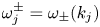 $\omega _j^\pm =\omega _\pm (k_j)$
 $(\,j=1,2,3)$ being assumed to be positive. To be shown later, the 1-D class-I and class-III resonances can be described as special cases of the type-A resonance defined by (2.2). Similarly, the 1-D class-II resonance between one surface and two internal wave modes propagating in opposite directions (Segur Reference Segur1980) is a part of the class-B resonance. Therefore, the 1-D resonances will not be considered separately here.
To examine the resonance conditions (2.2) and (2.3) with (2.1), we non-dimensionalize all physical variables with respect to  $\rho _1$,
 $g$ and
 $h_1$ so that the dimensionless dispersion relations can be written, from (2.1), as
 \begin{equation} \varOmega_{\pm}^2= \frac{\rho K}{2(T_1T_2+\rho)} \left[T_1 + T_2 \pm \sqrt{(T_1 + T_2 )^2-4(\rho-1)(T_1T_2+\rho)T_1T_2/\rho^2}\right], \end{equation}
where  $\varOmega _{\pm }=(h_1/g)^{1/2}\omega _{\pm }$,
 $K=kh_1$,
 $T_1 = \tanh (K)$,
 $T_2 = \tanh (Kh)$,
 $\rho = \rho _2/\rho _1>1$ and
 $h=h_2/h_1$. Note that the dispersion relations depend on two physical parameters
 $\rho$ and
 $h$, which are the density and depth ratios, respectively. Then the dimensionless resonance conditions can be written, from (2.2) and (2.3), as
 \begin{gather} \boldsymbol{K}_1 =\boldsymbol{K}_2 +\boldsymbol{K}_3 , \end{gather}
 \begin{gather}\varOmega_1=\varOmega_2+ \varOmega_3, \end{gather}
where  $\boldsymbol {K}_j=\boldsymbol {k}_j h_1$ with
 $K_j=\vert \boldsymbol {K}_j\vert >0$ and
 $\varOmega _j=\varOmega (K_j)>0$. Next, the wavenumber vectors satisfying the 2-D resonance conditions (2.5) and (2.6) will be described in detail, focusing on the spectral domain of resonance, where resonant triads can always be found.
2.1. Spectral domain of triad resonance
When the dimensionless wavenumber vectors  $\boldsymbol {K}_j$
 $(\,j=1,2,3)$ are expressed, in polar form, as
 $\boldsymbol {K}_j = K_j(\cos \theta _j,\sin \theta _j)$, three of the six unknowns (
 $K_j$ and
 $\theta _j$ for
 $j=1,2,3$) are free to choose as the resonance conditions (2.5) and (2.6) yield three scalar equations. After assuming, without loss of generality, that
 $\boldsymbol {K}_1$ is aligned with the
 $x$-axis (
 $\theta _1=0$), the resonance conditions for the three wavenumber vectors given by (2.5) can be rewritten as
 \begin{equation} K_1= K_2\cos\theta_2 + K_3\cos\theta_3,\quad 0= K_2\sin\theta_2 + K_3\sin\theta_3, \end{equation}
where  $\sin \theta _2$ and
 $\sin \theta _3$ must have opposite signs or be zeros with
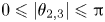 $0\leqslant \vert \theta _{2,3}\vert \leqslant {\rm \pi}$. Then, by fixing two additional free parameters, the solutions of (2.6) and (2.7a,b) can be found. In this study,
 $K_2$ and
 $K_3$ are chosen as the two free parameters.
Then, from (2.6),  $K_1$ can be expressed in terms of
 $K_2$ and
 $K_3$ and, from (2.7a,b), the expressions for
 $\theta _2$ and
 $\theta _3$ can be found as
 \begin{equation} \cos\theta_2 = \frac{K_1^2+K_2^2-K_3^2}{2K_1K_2}, \quad \cos\theta_3 = \frac{K_1^2+K_3^2-K_2^2}{2K_1K_3}. \end{equation}
Given that  $|\cos \theta _j|\leqslant 1$, one can see from (2.8a,b) that
 $K_j$ satisfy the following inequalities:
 \begin{equation} \vert K_1-K_2\vert \leqslant K_3 \leqslant K_1+K_2, \quad \vert K_1-K_3\vert \leqslant K_2 \leqslant K_1+K_3 . \end{equation}
In the three-dimensional  $(K_1,K_2,K_3)$-space, the volumes represented by the two inequalities are identical and define an open tetrahedron originating from the origin and bounded by three planes defined by
 \begin{equation} K_1= - K_2+ K_3 ,\quad K_1= K_2 - K_3,\quad K_1= K_2+ K_3. \end{equation}
Therefore, all resonant triads must have  $K_j$ (
 $\,j=1,2,3$) inside the open tetrahedron,
 ${T}$. If
 $(0,\theta _2,\theta _3)$ are the propagation directions of three waves in a resonant triad,
 $(0,-\theta _2,-\theta _3)$ are also possible propagation angles, but the corresponding resonant triad is simply the mirror image of the original triad about the
 $K_1$-axis. The equalities in (2.9a,b) hold only when
 $(\theta _{2},\theta _{3}) = (0,0)$,
 $(0,{\rm \pi} )$, or
 $({\rm \pi} ,0)$, which implies that 1-D resonant triads must appear on the faces of
 $T$ defined by (2.10a–c). Additionally, from (2.7a,b), one can see that
 $\theta _2=-\theta _3$ only when (i)
 $K_2=K_3$ or (ii)
 $K_1=K_2+K_3$, the latter of which implies 1-D waves with
 $\theta _2=\theta _3=0$.
The resonance condition between the wave frequencies  $\varOmega _j$ (
 $\,j=1,2,3$) given by (2.6) can be written, after using the linear dispersion relations, in the form of
 $F(K_1, K_2, K_3)=0$, which defines a surface
 $S$ in the
 $(K_1,K_2,K_3)$-space. Then, any part of
 $S$ residing inside
 $T$ defines the surface of resonance
 $S_R$.
As the dispersion relations for surface and internal gravity waves are different, to explicitly find the resonance surface  $S_R$, the resonance condition between
 $\varOmega _j$ (
 $\,j=1,2,3$) given by (2.6) needs to be examined separately for the type-A and type-B resonances.
2.2. Type-A resonance between two surface waves and one internal wave
For the type-A resonance, we consider two surface wave modes 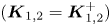 $(\boldsymbol {K}_{1,2} = \boldsymbol {K}_{1,2}^+)$ and one internal wave mode
 $(\boldsymbol {K}_3 = \boldsymbol {K}_3^-)$ that satisfy the resonance conditions
 \begin{equation} \boldsymbol{K}_1^+ =\boldsymbol{K}_2^+ +\boldsymbol{K}_3^-,\quad \varOmega_1^+ = \varOmega_2^+ + \varOmega_3^-, \end{equation}
where the superscript  $+$ or
 $-$ for
 $\boldsymbol {K}_j$ (
 $\,j=1,2,3$) is used just to emphasize that the wavenumber is associated with either the surface or internal wave mode while
 $\varOmega _j^\pm$ are defined by
 \begin{equation} \varOmega_j^\pm = \varOmega_\pm(K_j). \end{equation}
Figure 2 $(a)$ shows the surface
 $S$ and the open tetrahedron
 $T$ defined by (2.6) and (2.10a–c), respectively, for
 $h_2/h_1=4$ and
 $\rho _2/\rho _1=1.163$. The resonance surface denoted by
 $S_R$ is the part of
 $S$ inside
 $T$ and, then, all possible resonant triads stay on
 $S_R$.
Type-A resonance. ( $a$) Surface
 $S$ in the
 $(K_1^+,K_2^+,K_3^-)$-space defined by the resonance condition for the wave frequencies (2.6) for
 $\rho _2/\rho _1=1.163$ and
 $h_2/h_1=4$. The dashed lines represent the edges of
 $T$. (
 $b$) Region of type-A resonance (shaded), which is the projection of the resonance surface
 $S_R$ onto the
 $(K_2^+,K_3^-)$-plane. The boundaries (dashed) represent the 1-D class-I and class-III resonant interactions. The black dot on the abscissa denotes the minimum wavenumber for the 1-D class-III resonance:
 $K_{2m}^+\approx 2.157$. The long dashed line represents the symmetric case of
 $K_2^+=K_3^-$ and
 $\theta _2^+=-\theta _3^-$.

When  $K_2^+$ and
 $K_3^-$ are chosen as two free parameters, the projection of
 $S_R$ onto the
 $(K_2^+, K_3^-)$-plane is shown in figure 2
 $(b)$, where
 $K_j^\pm = \vert \boldsymbol {K}_j^\pm \vert$
 $(\,j=2,3)$. For any choice of
 $(K_2^+, K_3^-)$ inside the shaded area, which will be referred to as the resonance region,
 $K_1^+$ and
 $\theta _j^\pm$ (
 $\,j=2,3$) can be computed from (2.6) and (2.8a,b). Then, the corresponding resonant triad can be constructed inside the resonance region.
The boundaries (in dashed lines) of the resonance region represent 1-D resonant triad interactions. The upper boundary corresponds to the intersection of the resonance surface  $S_R$ with the plane given by
 $K_1^+= -K_2^+ +K_3^-$ so that, from (2.8a,b),
 $\theta _2^+={\rm \pi}$ and
 $\theta _3^-=0$. Therefore, along with
 $\theta _1^+=0$, the upper boundary describes the 1-D class-I resonance, where the two surface wave modes are propagating in opposite directions. As can be seen in figure 2
 $(b)$, the 1-D class-I resonance is possible for any value of
 $K_2^+$.
On the other hand, the lower boundary in figure 2 $(b)$ represents the intersection of
 $S_R$ with the plane given by
 $K_1^+=K_2^+ +K_3^-$ for which
 $\theta _2^+=\theta _3^-=0$ from (2.8a,b) so that the two surface and one internal waves propagate in the same direction. This is known as the 1-D class-III resonance and occurs only when at least one of the surface wavenumbers (more specifically,
 $K_1^+$ in our case) is greater than the critical wavenumber
 $K_c^+$ whose group velocity is the same as the phase velocity of a long internal wave. The critical wavenumber
 $K_c^+$ depends on the density and depth ratios and, for the physical parameters used in figure 2,
 $K_c^+\approx 2.17$. For 1-D waves, note that the class-III resonance (
 $K_1^+=K_2^+ +K_3^-$) occurs only when
 $K_2^+>K_3^-$, while the class-I resonance (
 $K_1^++K_2^+ = K_3^-$) occurs when an internal wave has a shorter wavelength than two surface waves (
 $K_3^->K_{1,2}^+)$.
For 2-D type-A resonant triads, the solutions of (2.11a,b) for different values of  $K_3^-$ are shown in figure 3. One can see from figure 3
 $(a)$ that
 $K_1^+$ in general increases with
 $K_2^+$ for a fixed value of
 $K_3^-$. The range of
 $K_2^+$ is bounded by
 $(K_2^+)_{min}$ and
 $(K_2^+)_{max}$, which correspond to the values of
 $K_2^+$ for the 1-D class-I and class-III resonances, respectively. As can be seen from figure 3
 $(b)$, for
 $K_3^-=1$, the propagation angle
 $\theta _2^+$ decreases from
 ${\rm \pi}$ to 0 as
 $K_2^+$ increases while
 $\theta _3^-$ remains negative. In general, when
 $K_3^-$ is fixed,
 $\theta _2^+> -\theta _3^-$ for
 $(K_2^+)_{min}<K_2^+ < K_3^-$ while the opposite is true for
 $K_3^-<K_2^+ < (K_2^+)_{max}$.
Type-A resonant triads for  $\rho _2/\rho _1=1.163$ and
 $h_2/h_1=4$. (
 $a$)
 $K_1^+$ versus
 $K_2^+$ (solid) for different values of
 $K_3^-$. The dashed and dash–dotted lines represent the 1-D class-I and class-III resonances, respectively. (
 $b$)
 $\theta _2^+$ (solid) and
 $-\theta _3^-$ (dashed) versus
 $K_2^+$ for
 $K_3^-=1$, for which the range of
 $K_2^+$ is given by
 $0.337\lesssim K_2^+\lesssim 3.398$. Note that
 $\theta _1^+=0$.

As pointed out previously, when  $K_2^+=K_3^-$, we have
 $\theta _2^+=-\theta _3^-$ so that a surface wave mode and an internal wave mode are propagating symmetrically about the positive
 $x$-axis, which is the propagation direction of the
 $K_1^+$ wave. For example, the propagation angle for the symmetric case with
 $K_3^-=1$ is approximately
 $38.19^{\circ }$, as shown in figure 3
 $(b)$. In fact, the propagation angle for the symmetric triad varies slightly with
 $K_3^-$ and its limiting value as
 $K_3^-\to \infty$ can be estimated, as follows. From (2.4), for large
 $K$, the dispersion relations can be approximated by
 \begin{equation} \varOmega_\pm^2 \simeq \left(\frac{\rho\pm 1}{\rho+1}\right ) K, \end{equation}
where  $\rho =\rho _2/\rho _1>1$, and
 $T_j\to 1$ (
 $\,j=1,2$) as
 $K\to \infty$ have been used. Then, for the type-A symmetric resonance with
 $K_2^+=K_3^-$, we have, from (2.11a,b),
 \begin{equation} K_1^+=K_3^-\left ( 1+\sqrt{\frac{\rho- 1}{\rho+1}}\right)^2,\quad \cos\theta_2^+=\frac{K_1^+}{2K_3^-}=\frac{1}{2}\left ( 1+\sqrt{\frac{\rho- 1}{\rho+1}}\right )^2. \end{equation}
For  $\rho =\rho _2/\rho _1=1.163$, the symmetric triad with
 $K_2^+=K_3^-$ has
 $K_1^+/K_3^-\approx 1.624$ and
 $\theta _2\approx 35.71^{\circ }$ as
 $K_3^-\to \infty$.
For a density ratio close to one, relevant for the ocean, the qualitative characteristics of 2-D resonant triads are similar to those shown in figures 2 and 3, except for the value of  $K_{2m}^+$, at which the 1-D class-III resonance is originated from the
 $K_2^+$-axis, as shown in figure 2
 $(b)$. As discussed in Taklo & Choi (Reference Taklo and Choi2020), when the density ratio approaches one,
 $K_{2m}^+$ increases rapidly for the class-III resonance. For example, for
 $h_2/h_1=4$ and
 $\rho _2/\rho _1=1.01$, the minimum surface wavenumber for the 1-D class-III resonance is given by
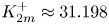 $K_{2m}^+\approx 31.198$.
In general, except for the areas near the  $K_2^+$ and
 $K_3^-$-axes, the 2-D type-A resonant triads can always be found in the
 $(K_2^+,K_3^-)$-plane.
2.3. Type-B resonance between one surface wave and two internal waves
The type-B resonance occurs between one surface and two internal wave modes. When we assume that  $\boldsymbol {K}_1 = \boldsymbol {K}_1^+$ and
 $\boldsymbol {K}_{2,3} = \boldsymbol {K}_{2,3}^-$, the resonance conditions are given by
 \begin{equation} \boldsymbol{K}_1^+ =\boldsymbol{K}_2^-+\boldsymbol{K}_3^-,\quad \varOmega_1^+ = \varOmega_2^- + \varOmega_3^- . \end{equation}
Figure 4 $(a)$ shows the surface
 $S$ defined by the resonance condition between
 $\varOmega _1^+$ and
 $\varOmega _{2,3}^-$ for
 $\rho _2/\rho _1=1.163$ and
 $h_2/h_1=4$. Again the part of
 $S$ inside the open tetrahedron
 $T$ defines the resonance surface
 $S_R$. Figure 4
 $(b)$ shows the region of resonance, or the projection of
 $S_R$ onto the
 $(K_2^-, K_3^-)$-plane. As the subscripts 2 and 3 in (2.15a,b) can be interchanged, one can expect the resonance region to be symmetric about the straight line
 $K_2^-=K_3^-$, as can be seen from figure 4
 $(b)$. The resonant triads on one side of the line of symmetry are equivalent to those on the other side when the subscripts 2 and 3 are interchanged.
Type-B resonance for  $\rho _2/\rho _1=1.163$ and
 $h_2/h_1=4$. (
 $a$) Surface
 $S$ in the
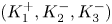 $(K_1^+,K_2^-,K_3^-)$-space defined by the resonance condition for the wave frequencies given by (2.6). The dashed lines represent the edges of
 $T$. (
 $b$) Region of type-B resonance (shaded), which is the projection of the resonance surface
 $S_R$ onto the
 $(K_2^-, K_3^-)$-plane. The short-dashed lines represent the 1-D class-II resonant interactions and, as the subscripts 2 and 3 can be changed, the region is symmetric about the long-dashed line, on which symmetric resonant triads of type-B exist with
 $K_2^-=K_3^-$ and
 $\theta _2^-=-\theta _3^-$.

Once again, the boundaries of the resonance region (shaded) in figure 4 $(b)$ represent 1-D resonant interactions. The upper and lower boundaries correspond to the intersections of
 $S$ with the planes given by
 $K_1^+=-K_2^-+K_3^-$ and
 $K_1^+=K_2^--K_3^-$, respectively. As the propagation angles on the upper and lower boundaries are given, from (2.8a,b), by
 $(\theta _2^-,\theta _3^-)=({\rm \pi} ,0)$ and
 $(\theta _2^-,\theta _3^-)=(0,{\rm \pi} )$, respectively, two internal waves in a resonant triad propagate in opposite directions to each other while the surface wave with
 $\theta _1^+=0$ propagates in the positive
 $x$-direction. This is known as the 1-D class-II resonance (Segur Reference Segur1980).
Figure 5 $(a)$ shows the variation of
 $K_1^+$ with
 $K_2^-$ for different values of
 $K_3^-$. For each value of
 $K_3^-$, the admissible range of
 $K_2^-$ is limited by the 1-D class-II resonance and increases with
 $K_3^-$. For example, for
 $K_3^-=4$, the type-B resonance occurs only for
 $2.960\lesssim K_2^-\lesssim 5.408$. The surface wavenumber
 $K_1^+$ increases with
 $K_2^-$ in the range, but remains smaller than both
 $K_2^-$ and
 $K_3^-$. Therefore, the type-B resonance is the interaction between a longer surface wave and two shorter internal waves. Due to the symmetry between the subscripts 2 and 3 in the resonance conditions given by (2.15a,b), the propagation angles for the
 $K_2^-$ and
 $K_3^-$ waves (
 $\theta _{2,3}^-$) are reversed when
 $K_2^-=K_3^-$, as shown in figure 5
 $(b)$.
Type-B resonant triads for  $\rho _2/\rho _1=1.163$ and
 $h_2/h_1=4$. (
 $a$)
 $K_1^+$ versus
 $K_2^-$ for different values of
 $K_3^-$. The upper and lower dashed lines represent the 1-D class-II resonances with
 $(\theta _2^-,\theta _3^-)=({\rm \pi} ,0)$ and
 $(\theta _2^-,\theta _3^-)=(0,{\rm \pi} )$, respectively. Note that
 $\theta _1^+=0$. (
 $b$)
 $\theta _2^-$ (solid) and
 $-\theta _3^-$ (dashed) versus
 $K_2^-$ for
 $K_3^-=4$. The admissible range of
 $K_2^-$ is given by
 $2.960\lesssim K_2^-\lesssim 5.408$, whose limits are the two possible values of
 $K_2^-$ for the 1-D class-II resonance.

Similarly to the type-A case, the type-B resonance also supports symmetric triads with  $K_2^-=K_3^-$ and
 $\theta _2^-=-\theta _3^-$, as shown in figure 4
 $(b)$. The surface wavenumber
 $K_1^+$ in a symmetric triad increases with
 $K_2^-$ and its limiting behaviour as
 $K_2^-\to \infty$ can be found, from the frequency resonance condition for the symmetric case given by
 $\varOmega _+(K_1^+)=2\varOmega _-(K_2^-)$ with (2.13) for
 $\varOmega _\pm$, as
 \begin{equation} {K_1^+/K_2^-}=4(\rho-1)/(\rho+1). \end{equation}
On the other hand, the propagation angle  $\theta _2=-\theta _3$ can be found, from (2.8a,b), as
 \begin{equation} \cos\theta_2=K_1^+/(2K_2^-)=2(\rho-1)/(\rho+1). \end{equation}
For example, for  $\rho _2/\rho _1=1.163$, the propagation directions of two symmetric internal waves about the
 $x$-axis are close to
 ${\pm }81.34^{\circ }$, independent of the depth ratio, while the surface wave is propagating in the positive
 $x$-direction.
When the density ratio  $\rho _2/\rho _1$ approaches 1, the width of the resonance region decreases toward the line of symmetry
 $K_2^-=K_3^-$. Therefore, the type-B resonance is expected to less frequently occur under realistic oceanic conditions unless the wave frequencies satisfy
 $\varOmega _1^+\approx 2\varOmega _2^- \approx 2\varOmega _3^-$. For the symmetric resonance to occur, the propagation angles of the two internal waves are close to
 ${\pm }90^{\circ }$, as can be seen from (2.17), so that the surface and internal waves are propagating almost perpendicularly to each other.
As the density ratio  $\rho _2/\rho _1$ increases from 1, the resonance region first widens, but, beyond a certain density ratio, a qualitatively different region of resonance appears. For example, figure 6 shows the resonance surface
 $S_R$ and its projection onto the
 $(K_2^-,K_3^-)$-plane for
 $\rho _2/\rho _1=3.1$ and
 $h_2/h_1=4$. The symmetric resonant triad disappears at a finite value of
 $K_2^-$, where the resonance region is split and is bounded by two outer and two inner boundaries. The outer boundaries still correspond to the 1-D class-II resonance, but the inner boundaries that appear on the face of the open tetrahedron given by
 $K_1^+=K_2^-+K_3^-$ represent a different 1-D resonance. The corresponding propagation angles can be found, from (2.8a,b), as
 $\theta _1^+=\theta _2^-=\theta _3^-=0$ and, therefore, all three waves propagate in the same direction, similarly to the 1-D class-III resonance observed in the type-A resonance. This resonance will be hereafter referred to as the 1-D class-IV resonance to distinguish it from other 1-D resonances.
Type-B resonance for  $\rho _2/\rho _1=3.1$ and
 $h_2/h_1=4$. (
 $a$) Surface
 $S$ in the
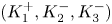 $(K_1^+,K_2^-,K_3^-)$-space defined by the resonance condition for the wave frequencies given by (2.6). The dashed lines represent the edges of
 $T$. (
 $b$) Resonance region (shaded) that is the projection of the resonance surface
 $S_R$ onto the
 $(K_2^-, K_3^-)$-plane. The short-dashed lines represent the 1-D class-II and class-IV resonant interactions. The dotted line denotes the symmetric triad resonance.

To find the critical density ratio beyond which the 1-D class-IV resonance occurs, it is sufficient to consider the short-wave limit as the class-IV resonance is always observed as  $K_j\to \infty$
 $(\,j=1,2,3)$, as shown in figure 6. For short waves, using the dispersion relations given by (2.13) for
 $\varOmega _\pm$, the class-IV resonance conditions can be written as
 \begin{equation} K_1^+=K_2^-+K_3^-,\quad \sqrt{K_1^+}=\sqrt{\frac{\rho-1}{\rho+1}} \left (\sqrt{K_2^-}+\sqrt{K_3^-} \right ), \end{equation}
which can be combined to
 \begin{equation} \left (\sqrt{K_2^-}-\sqrt{K_3^-} \right )^2/\sqrt{K_2^- K_3^-}=\rho-3 \geqslant 0. \end{equation}
Therefore, the 1-D class-IV resonance occurs only for  $\rho =\rho _2/\rho _1\geqslant 3$. Then the three waves propagate in the same direction.
From figure 6 $(b)$, it can be noticed that there exists a critical wavenumber
 $K_c^-$, where the symmetric triad ceases to exist and the class-IV resonance appears. At the criticality, from
 $K_2^-=K_3^-=K_c^-$ and
 $K_1^+=K_2^-+K_3^-=2K_c^-$, the critical wavenumber
 $K_c^-$ can be computed from the frequency condition for the class-IV resonance:
 $\varOmega _+(2K_c^-)=2\varOmega _-(K_c^-)$. For example, for
 $\rho _2/\rho _1=3.1$ and
 $h_2/h_1=4$, the critical wavenumber
 $K_c^-$ for the class-IV resonance can be computed as
 $K_c^- \approx 2.072$.
Figure 7 $(a)$ shows the variations of
 $K_1^+$ with
 $K_2^-$ for different values of
 $K_3^-$. For
 $K_3^- < K_{3m}^-\ ({\approx }1.940)$, the type-B resonance is possible over a range of
 $K_2^-$ bounded by the 1-D class-II resonances. For example, for
 $K_3^-=1$, the range of
 $K_2^-$ is given by
 $0.272 \lesssim K_2^-\lesssim 8.357$ and
 $K_1^+$ increases with
 $K_2^-$. The propagation angle of the
 $K_2^-$ wave decreases continuously from
 $\theta _2^-={\rm \pi}$ to 0 while the opposite is true for the
 $K_3^-$ wave, as shown in figure 7
 $(b)$. As before, the two propagation angles are the same for the symmetric case with
 $K_2^-=K_3^-$. On the other hand, for
 $K_3^-> K_{3m}^-$, the type-B resonance occurs over two ranges of
 $K_2^-$, each bounded by the 1-D class-II and class-IV resonances. For example, for
 $K_3^-=4$, the admissible ranges of
 $K_2^-$ are given by
 $0.580 \lesssim K_2^-\lesssim 2.337$ and
 $7.488 \lesssim K_2^-< \infty$, as can be observed in figure 7
 $(c)$. At
 $K_2^- \approx 2.337$ and 7.488, where the 1-D class-IV resonance happens,
 $\theta _2^-=\theta _3^-=0$, which implies, with
 $\theta _1^+=0$, that both the surface and internal waves propagate in the positive
 $x$-direction, as mentioned previously.
Type-B resonant triads for  $\rho _2/\rho _1=3.1$ and
 $h_2/h_1=4$. (
 $a$)
 $K_1^+$ versus
 $K_2^-$ for different values of
 $K_3^-$. The dashed and dash–dotted lines represent the class-II and class-IV resonances, respectively.
 $(b)$
 $\theta _2^-$ (solid) and
 $-\theta _3^-$ (dashed) versus
 $K_2^-$ for
 $K_3^-=1$. The admissible range of
 $K_2^-$ is given by
 $0.272 \lesssim K_2^-\lesssim 8.357$.
 $(c)$
 $\theta _2^-$ (solid) and
 $-\theta _3^-$ (dashed) versus
 $K_2^-$ for
 $K_3^-=4$. The admissible ranges of
 $K_2^-$ are given by
 $0.580 \lesssim K_2^-\lesssim 2.337$ and
 $7.488 \lesssim K_2^-< \infty$.

3. Spectral formulation for two-layer system
3.1. Two-layer Hamiltonian system
For a two-layer system shown in figure 1, it has been known (Benjamin & Bridges Reference Benjamin and Bridges1997; Craig, Guyenne & Kalisch Reference Craig, Guyenne and Kalisch2005) that the surface and interface motions are governed by a Hamiltonian system ( $i=1,2$):
 \begin{equation} \frac{\partial \zeta_i}{\partial t} =\frac{\delta E}{\delta \varPsi_i},\quad \frac{\partial \varPsi_i}{\partial t} =-\frac{\delta E}{\delta \zeta_i}. \end{equation}
Here the Hamiltonian  $E$ is the total energy. In (3.1a,b),
 $\zeta _1(\boldsymbol {x},t)$ and
 $\zeta _2(\boldsymbol {x},t)$ with
 $\boldsymbol {x}=(x,y)$ represent the surface and interface displacements, respectively, while
 $\varPsi _i(\boldsymbol {x},t)$
 $(i=1,2)$ are the density-weighted velocity potentials defined as
 \begin{equation} \varPsi_1= \rho_1\varPhi_1,\quad \varPsi_2= \rho_2\varPhi_2-\rho_{1}\bar \varPhi_{1}, \end{equation}
where  $\varPhi _1(\boldsymbol {x},t) \equiv \phi _1(\boldsymbol {x}, z=\zeta _1,t)$,
 $\bar \varPhi _1(\boldsymbol {x},t) \equiv \phi _1(\boldsymbol {x}, z=-h_1+\zeta _2,t)$ and
 $\varPhi _2(\boldsymbol {x},t) \equiv \phi _2(\boldsymbol {x}, z=-h_1+\zeta _2,t)$ with
 $\phi _i$
 $(i=1,2)$ being the solution of the three-dimensional Laplace equation of the
 $i$-th layer. Alternatively, one can define
 $\varPsi _1=\varPhi _1$ and
 $\varPsi _2=\varPhi _2-(\rho _2/\rho _1)\varPhi _1$, which is equivalent to considering
 $\rho _2$ as the density ratio with
 $\rho _1=1$ in the following formulations.
Under the assumption of small wave steepness,  $\epsilon \ll 1$, Taklo & Choi (Reference Taklo and Choi2020) obtained an explicit Hamiltonian system, correct to
 $O(\epsilon ^2)$, for
 $\zeta _i$ and
 $\varPsi _i$ (
 $i=1,2$) given by
 \begin{align} \frac{\partial \zeta_1}{\partial t}& = \gamma_{11}\varPsi_1+\gamma_{12}\varPsi_2 -\rho_1\, \gamma_{11}\left [\zeta_1 \left (\gamma_{11}\varPsi_1+\gamma_{12}\varPsi_2 \right)\right ] -{\rm \Delta} \rho\, \gamma_{21}\left [ \zeta_2\left(\gamma_{21}\varPsi_1+\gamma_{22}\varPsi_2\right)\right ]\nonumber\\ &\quad - \boldsymbol{\nabla}\boldsymbol{\cdot} (\zeta_1\boldsymbol{\nabla}\varPsi_1)/\rho_1 +{\rm \Delta} \rho(\rho_2/\rho_1 ) \gamma_{31} \boldsymbol{\nabla}\boldsymbol{\cdot} \left (\zeta_2 \gamma_{31} \boldsymbol{\nabla}\varPsi_1\right) -\rho_2 \gamma_{31} \boldsymbol{\nabla}\boldsymbol{\cdot} \left( \zeta_2 \gamma_{33} \boldsymbol{\nabla}\varPsi_2 \right), \end{align}
 \begin{align} \frac{\partial \zeta_2}{\partial t} &= \gamma_{21}\varPsi_1+\gamma_{22}\varPsi_2 -\rho_1\gamma_{12}\left [\zeta_1\left(\gamma_{11}\varPsi_1+\gamma_{12}\varPsi_2\right)\right ] -{\rm \Delta} \rho\gamma_{22}\left [\zeta_2\left(\gamma_{21}\varPsi_1+\gamma_{22}\varPsi_2\right)\right ]\nonumber\\ &\quad -\rho_2 \gamma_{33}\boldsymbol{\nabla}\boldsymbol{\cdot} (\zeta_2 \gamma_{31} \boldsymbol{\nabla}\varPsi_1) -\rho_2 J\boldsymbol{\nabla}\boldsymbol{\cdot} (\zeta_2 J\boldsymbol{\nabla}\varPsi_2) +\rho_1 \gamma_{32} \boldsymbol{\nabla}\boldsymbol{\cdot} (\zeta_2 \gamma_{32} \boldsymbol{\nabla}\varPsi_2) , \end{align}
 \begin{align} \frac{\partial \varPsi_1}{\partial t} &=- \rho_1 g\zeta_1 +\tfrac{1}{2} \rho_1\left (\gamma_{11}\varPsi_1+\gamma_{12}\varPsi_2\right)^2 -\tfrac{1}{2} \boldsymbol{\nabla}\varPsi_1\boldsymbol{\cdot}\boldsymbol{ \nabla}\varPsi_1/\rho_1, \end{align}
 \begin{align} \frac{\partial \varPsi_2 }{\partial t}&=-{\rm \Delta} \rho g\zeta_2 +\tfrac{1}{2} {\rm \Delta} \rho (\gamma_{21} \varPsi_1+\gamma_{22} \varPsi_2)^2 +\tfrac{1}{2} {\rm \Delta} \rho (\rho_2/\rho_1) (\gamma_{31} \boldsymbol{\nabla}\varPsi_1)\boldsymbol{\cdot}(\gamma_{31} \boldsymbol{\nabla} \varPsi_1)\nonumber\\ &\quad -\tfrac{1}{2} \rho_2 (J\boldsymbol{\nabla}\varPsi_2)\boldsymbol{\cdot} (J\boldsymbol{\nabla}\varPsi_2) +\tfrac{1}{2} \rho_1 (\gamma_{32}\boldsymbol{\nabla}\varPsi_2)\boldsymbol{\cdot} (\gamma_{32} \boldsymbol{\nabla}\varPsi_2) -\rho_2(\gamma_{31} \boldsymbol{\nabla}\varPsi_1)\boldsymbol{\cdot} (\gamma_{33} \boldsymbol{\nabla}\varPsi_2), \end{align}
where the Fourier multipliers  $\gamma _{ij}$ are defined as
 \begin{gather} \gamma_{11}=kJ\left [ (\rho_2 /\rho_1) T_1+ T_2\right] ,\quad \gamma_{12}=\gamma_{21}=k J S T_2,\quad \gamma_{22}=kJ{T_2}, \end{gather}
 \begin{gather} \gamma_{31}=JS,\quad \gamma_{32}=JT_1T_2,\quad \gamma_{33}=J(1+T_1T_2) , \end{gather}
with  $T_i$
 $(i=1,2)$,
 $S$ and
 $J$ given by
 \begin{equation} T_i =\tanh kh_i,\quad S=\textrm{sech}\,kh_1, \quad J=\left (\rho_1T_1T_2+\rho_2\right )^{-1}. \end{equation}
Here  $\gamma _{ij}\varPsi _l$ (
 $i,j=1,2,3$,
 $l=1,2$) should be understood as
 \begin{equation} \gamma_{ij}\varPsi_l=\varGamma_{ij}[\varPsi_l]\equiv \int_{-\infty}^{\infty} \hat\gamma_{ij}(\boldsymbol{x}-\boldsymbol{x}') \varPsi_l(\boldsymbol{x}',t)\, \textrm{d} \boldsymbol{x}', \end{equation}
where  $\hat \gamma _{ij}(\boldsymbol {x})$ is the inverse Fourier transform of
 $\gamma _{ij}(\boldsymbol {k})$. The similar interpretation also applies to
 $J\varPsi _l$ (
 $l=1,2$) in (3.4) and (3.6).
The corresponding Hamiltonian that is the total energy  $E$ can be written as
 \begin{equation} E=E_2+E_3, \end{equation}
where  $E_n=O(\epsilon ^n)$ are given by
 \begin{align} E_2&=\tfrac{1}{2}\int \left [ \rho_1 g{\zeta_1}^2+{\rm \Delta} \rho g {\zeta_2}^2 \right .\nonumber\\ &\quad \left. + \varPsi_1 (\gamma_{11}\varPsi_1 ) + \varPsi_1 (\gamma_{12} \varPsi_2) + \varPsi_2 (\gamma_{21} \varPsi_1) + \varPsi_2 (\gamma_{22} \varPsi_2) \right ] \textrm{d} \boldsymbol{x} , \end{align}
 \begin{align} E_3& =-\tfrac{1}{2}\int \left [ \zeta_1\left \{-\boldsymbol{\nabla}\varPsi_1\boldsymbol{\cdot} \boldsymbol{\nabla}\varPsi_1/\rho_1 + \rho_1 \left (\gamma_{11}\varPsi_1+\gamma_{12}\varPsi_2 \right )^2 \right \}\right . \nonumber\\ &\quad +\zeta_2\left \{ {\rm \Delta} \rho (\rho_2/\rho_1) (\gamma_{31}\boldsymbol{\nabla}\varPsi_1 )\boldsymbol{\cdot} (\gamma_{31} \boldsymbol{\nabla}\varPsi_1 ) -2\rho_2 (\gamma_{31} \boldsymbol{\nabla}\varPsi_1 )\boldsymbol{\cdot} \left(\gamma_{33}\boldsymbol{\nabla} \varPsi_2 \right)\right .\nonumber\\ &\quad \left.\left. +\rho_1 (\gamma_{32}\boldsymbol{\nabla} \varPsi_2 )\boldsymbol{\cdot} (\gamma_{32}\boldsymbol{\nabla} \varPsi_2 ) -\rho_2 (J\boldsymbol{\nabla} \varPsi_2 )\boldsymbol{\cdot} ( J\boldsymbol{\nabla} \varPsi_2 ) +{\rm \Delta} \rho (\gamma_{21}\varPsi_1+\gamma_{22}\varPsi_2 )^2 \right \} \right ] \textrm{d} \boldsymbol{x}. \end{align}
Then, it can be shown that the nonlinear evolution equations for  $\zeta _i$ and
 $\varPsi _i$ (
 $i=1,2)$ given by (3.3)–(3.6) are Hamilton's equations (3.1a,b). Therefore, the total energy given by (3.11) with (3.12) and (3.13) is conserved exactly.
While the resonant interactions between surface and internal wave modes are of our interest, the Hamiltonian system in physical space given by (3.3)–(3.6) describes the combined surface and interface motions of the two modes. Therefore, it is necessary to identify the surface and internal wave contributions from the surface and interface motions. As this decomposition can be accomplished conveniently in spectral space, we first obtain a spectral model corresponding to the Hamiltonian system (3.3)–(3.6).
3.2. Hamiltonian in spectral space
To write the second-order model in spectral space, we introduce the Fourier transforms of  $\zeta _j$ and
 $\varPsi _j$ (
 $\,j=1,2$):
 \begin{equation} \zeta_{1, 2}(\boldsymbol{x},t)=\int a_{+, -} (\boldsymbol{k},t)\, \textrm{e}^{- \textrm{i}\boldsymbol{k}{{\boldsymbol{\cdot}}}\boldsymbol{x}} \, \textrm{d}\boldsymbol{k},\quad \varPsi_{1, 2} (\boldsymbol{x},t)=\int b_{+, -} (\boldsymbol{k},t)\, \textrm{e}^{- \textrm{i}\boldsymbol{k}{{\boldsymbol{\cdot}}}\boldsymbol{x}} \,\textrm{d}\boldsymbol{k}.\end{equation}
As  $\zeta _j$ and
 $\varPsi _j$ are real functions, the complex conjugates of
 $a_\pm$ and
 $b_\pm$, denoted by
 $a_\pm ^*$ and
 $b_\pm ^*$, satisfy
 \begin{equation} a_\pm^*(\boldsymbol{k}, t)=a_\pm(-\boldsymbol{k},t),\quad b_\pm^*(\boldsymbol{k}, t)=b_\pm(-\boldsymbol{k},t). \end{equation}
By substituting these into (3.12) and (3.13), the second- and third-order Hamiltonians (leading to the linear and second-order systems, respectively) defined by  $H_n=E_n/(2{\rm \pi} )^2$ can be found as
 \begin{align} H_2 & = \tfrac{1}{2} \int \left ( \rho_u g a_+ a_+^* +{\rm \Delta} \rho ga_- a_-^* + \gamma_{11 }b_+ b_+^* +\gamma_{12} b_+^*b_- +\gamma_{21} b_+b_-^* + \gamma_{22} b_- b_-^* \right ) \textrm{d}\boldsymbol{k}, \end{align}
 \begin{align} H_{3}&=\iiint \left [h^{(1)}_{1,2,3} b_1^+ b_2^+ a_3^+ +h^{(2)}_{1,2,3} b_1^+ b_2^- a_3^+ +h^{(3)}_{1,2,3} b_1^- b_2^- a_3^+\right .\nonumber\\ &\quad \left. +h^{(4)}_{1,2,3} b_1^+ b_2^+ a_3^- +h^{(5)}_{1,2,3} b_1^+ b_2^- a_3^-+h^{(6)}_{1,2,3} b_1^- b_2^- a_3^- \right ] \delta_{1+2+3}\, \textrm{d}\boldsymbol{k}_{1,2,3}, \end{align}
where  $\delta (\boldsymbol {k})$ is the Dirac delta function with
 \begin{equation} \delta_j=\delta(\boldsymbol{k}_j),\quad \delta_{1+2}=\delta(\boldsymbol{k}_1+\boldsymbol{k}_2),\quad \delta_{1+2+3}=\delta(\boldsymbol{k}_1+\boldsymbol{k}_2+\boldsymbol{k}_3), \end{equation}
and we have used the following shorthand notation for  $j=1,2$:
 \begin{equation} a_j^\pm=a_\pm(\boldsymbol{k}_j),\quad b_j^\pm=b_\pm(\boldsymbol{k}_j), \quad \textrm{d}\boldsymbol{k}_{1,2,3} = \textrm{d}\boldsymbol{k}_1\, \textrm{d}\boldsymbol{k}_2\,\textrm{d}\boldsymbol{k}_3. \end{equation}
Note that, due to  $\delta _{1+2+3}$, the triple integral in (3.17) can be written as a double integral. In (3.16) and (3.17), as the subscripts are used to denote the wavenumber dependence,
 $\rho _1$ and
 $\rho _2$ are replaced by
 $\rho _u$ and
 $\rho _l$, respectively, and the superscripts have been used for
 $\pm$ whenever necessary to avoid any confusion with the indices for wavenumbers. Likewise,
 $T_1$ and
 $T_2$ are replaced by
 $U$ and
 $L$ so that
 \begin{equation} U_j=\tanh (k_jh_1) ,\quad L_j=\tanh(k_jh_2), \quad J_j=\left (\rho_uU_jL_j +\rho_l\right )^{-1},\quad S_j=\textrm{sech}(k_jh_1). \end{equation}
The coefficients  $h^{(\,j)}_{1,2,3}$ for
 $j=1,2,\ldots , 6$ in (3.17) are defined as
 \begin{gather} h^{(1)}_{1,2,3} =-\tfrac{1}{2} (\boldsymbol{k}_1\cdot\boldsymbol{k}_2)/\rho_u-\textstyle\frac{1}{2} \rho_u\gamma_{11,1} \gamma_{11,2}, \end{gather}
 \begin{gather}h^{(2)}_{1,2,3} =-\rho_u\gamma_{11,1}\gamma_{12,2}, \quad h^{(3)}_{1,2,3} =-\textstyle\frac{1}{2} \rho_u \gamma_{12,1}\gamma_{12,2} , \end{gather}
 \begin{gather}h^{(4)}_{1,2,3} =-\textstyle\frac{1}{2} {\rm \Delta} \rho \left[ -(\rho_l/\rho_u) \gamma_{31,1} \gamma_{31,2}(\boldsymbol{k}_1\boldsymbol{\cdot}\boldsymbol{k}_2) +\gamma_{21,1} \gamma_{21,2}\right ], \end{gather}
 \begin{gather}h^{(5)}_{1,2,3} = - {\rm \Delta} \rho \gamma_{21,1}\gamma_{22,2} - \rho_l \gamma_{31,1}\gamma_{33,2}(\boldsymbol{k}_1\boldsymbol{\cdot}\boldsymbol{k}_2) , \end{gather}
 \begin{gather}h^{(6)}_{1,2,3} =-\textstyle\frac{1}{2} \left [{\rm \Delta} \rho\gamma_{22,1}\gamma_{22,2} +\left (\rho_l \gamma_{30,1}\gamma_{30,2}-\rho_u \gamma_{32,1}\gamma_{32,2}\right )(\boldsymbol{k}_1\boldsymbol{\cdot}\boldsymbol{k}_2) \right ] , \end{gather}
where  $\gamma _{mn,j}$ denote
 $\gamma _{mn}$ defined in (3.7a–c) with
 $k=k_j$ so that
 \begin{gather} \gamma_{11,j}=k_jJ_j\left [ (\rho_l /\rho_u) U_j+ L_j\right] ,\quad \gamma_{12,j}=\gamma_{21,j}= k_j J_j S_j L_j,\quad \gamma_{22,j}=k_j J_j L_j , \end{gather}
 \begin{gather} \gamma_{30,j}=J_j,\quad \gamma_{31,j}=J_j S_j,\quad \gamma_{32,j}=J_jU_jL_j,\quad \gamma_{33,j}=J_j(1+U_jL_j) . \end{gather}
Note that  $h^{(\,j)}_{1,2,3}$ satisfy the following conditions:
 \begin{gather} h^{(\,j)}_{1,2,3}=h^{(\,j)}_{2,1,3}\quad \mbox{for } j=1,3,4,6, \end{gather}
 \begin{gather}h^{(\,j)}_{1,2,3}=h^{(\,j)}_{-1,-2,3}=h^{(\,j)}_{1,2,-3}=h^{(\,j)}_{-1,-2,-3}\quad \mbox{for } j=1,\ldots,6 . \end{gather}
From Hamilton's equations in spectral space (Krasitskii Reference Krasitskii1994) with  $H=H_2+H_3$, the evolution equations for
 $a_\pm$ and
 $b_\pm$ can be obtained from
 \begin{equation} \frac{\partial a_\pm }{\partial t}=\frac{\delta H}{\delta b_\pm^*},\quad \frac{\partial b_\pm}{\partial t} =-\frac{\delta H}{\delta a_\pm^*}, \end{equation}
which are given explicitly in appendix A.
3.3. Mode decomposition into surface and internal wave modes
As  $a_\pm$ and
 $b_\pm$ represent the combined motions of the surface and internal wave modes, the system for
 $a_\pm$ and
 $b_\pm$ given by (3.30a,b), or, explicitly by (A 1) and (A 2), is inconvenient to study energy transfer between the two wave modes. Therefore, it is desirable to decompose
 $a_\pm$ and
 $b_\pm$ into the amplitudes of the two modes.
As described in detail in appendix B, one can find new conjugate variables 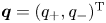 $\boldsymbol {q}=(q_+, q_-)^\textrm {T}$ and
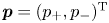 $\boldsymbol {p}=(p_+, p_-)^\textrm {T}$ from
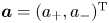 $\boldsymbol {a}=(a_+, a_-)^\textrm {T}$ and
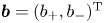 $\boldsymbol {b}=(b_+, b_-)^\textrm {T}$ using the transformation
 \begin{equation} \boldsymbol{a}=\boldsymbol{Qq},\quad\boldsymbol{b}=\boldsymbol{Pp}, \end{equation}
where  $\boldsymbol {Q}$ and
 $\boldsymbol {P}$ are
 $2\times 2$ matrices given by (B 16). Here
 $\boldsymbol {q}$ and
 $\boldsymbol {p}$ correspond to the generalized coordinate and momentum, respectively, with
 $(q_+, p_+)$ and
 $(q_-, p_-)$ describing the surface and internal wave modes, respectively. Note that
 $(\boldsymbol {q},\boldsymbol {p})$ and their complex conjugates are related as
 \begin{equation} \boldsymbol{q}(-{\boldsymbol{k}},t)=\boldsymbol{q}^*({\boldsymbol{k}},t),\quad \boldsymbol{p}(-\boldsymbol{k},t)=\boldsymbol{p}^*(\boldsymbol{k},t). \end{equation}
By substituting (B 16) into (3.16) (with the help of Mathematica), the second-order Hamiltonian  $H_2$ can be found, in terms of the conjugate variables (
 $q_\pm$,
 $p_\pm$), as
 \begin{equation} H_2=\tfrac{1}{2} \int \left [ \left(\omega_+^2 q_+q_+^* + p_+p_+^*\right) +\left (\omega_-^2 q_- q_-^* +p_- p_-^* \right)\right ] \textrm{d}\boldsymbol{k}, \end{equation}
where the sum of the first two terms and that of the last two terms represent the total energy of the surface and internal wave modes, respectively, under the linear assumption.
The expression for the third-order Hamiltonian  $H_3$ representing the nonlinear interactions between the surface and internal wave modes can be found, in terms of the conjugate variables (
 $q_\pm$,
 $p_\pm$), as
 \begin{align} H_{3}&=\iiint \left [U^{(1)}_{1,2,3} p_{1}^+ p_{2}^+q_{3}^+ +U^{(2)}_{1,2,3} p_{1}^+p_2^-q_3^+ +U^{(3)}_{1,2,3} p_1^- p_2^-q_3^+ \right .\nonumber\\ &\quad \left. +U^{(4)}_{1,2,3} p_{1}^+ p_{2}^+q_{3}^- +U^{(5)}_{1,2,3} p_1^+ p_2^-q_3^- +U^{(6)}_{1,2,3} p_1^- p_2^-q_3^- \right ] \delta_{1+2+3}\, \textrm{d}{\boldsymbol{k}}_{1,2,3} , \end{align}
where  $U^{(\,j)}_{1,2,3}$ for
 $j=1,\ldots , 6$ are listed in appendix C. Once again, we have used the superscripts
 $\pm$ to avoid any confusion with the indices for wavenumbers so that
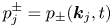 $p_j^{\pm }=p_\pm (\boldsymbol {k}_j,t)$ and
 $q_j^{\pm }=q_\pm (\boldsymbol {k}_j,t)$. From Hamilton's equations given by (B 15), or
 \begin{equation} \frac{\partial \boldsymbol{q}}{\partial t}=\frac{\delta H}{\delta \boldsymbol{p}^*},\quad \frac{\partial \boldsymbol{p}}{\partial t}=-\frac{\delta H}{\delta \boldsymbol{q}^*}, \end{equation}
one can find the evolution equations for  $(\boldsymbol {q}, \boldsymbol {p})$, which are explicitly given in (B 18)–(B 21).
3.4. Scalar complex amplitudes
Following Zakharov (Reference Zakharov1968) for surface waves, instead of using  $\boldsymbol {q}(\boldsymbol {k},t)$ and
 $\boldsymbol {p}(\boldsymbol {k},t)$, we introduce the following scalar complex amplitudes
 $z_\pm (\boldsymbol {k},t)$ for the surface and internal wave modes, respectively,
 \begin{equation} z_{\pm}(\boldsymbol{k},t)= \sqrt{\frac{\omega_\pm}{2}} \left [q_\pm (\boldsymbol{k},t)- \textrm{i} \frac{p_\pm(\boldsymbol{k},t)}{\omega_\pm}\right ], \end{equation}
from which  $q_\pm$ and
 $p_\pm$ can be written in terms of
 $z_\pm$ as
 \begin{align} q_\pm (\boldsymbol{k},t)=\sqrt{\frac{1}{2\omega_\pm}} \left[z_\pm (\boldsymbol{k},t) + z_\pm^*(-\boldsymbol{k},t) \right ] ,\quad p_\pm (\boldsymbol{k},t)=\textrm{i} \sqrt{\frac{\omega_\pm}{2}} \left [z_\pm(\boldsymbol{k},t) - z_\pm^*(-\boldsymbol{k},t) \right] , \end{align}
where we have used (3.32a,b), and  $\omega _\pm$ are assumed positive. Then,
 $z_\pm$ can be related to
 $(\boldsymbol {a},\boldsymbol {b})$ from (3.31a,b) with (3.37a,b).
By substituting (3.37a,b) into (3.33) and (3.34),  $H_2$ can be found, in terms of
 $z_\pm (\boldsymbol {k},t)$, as
 \begin{equation} H_2= \int \left(\omega_+ z_+ z_+^* + \omega_- z_- z_-^* \right) \textrm{d}\boldsymbol{k}, \end{equation}
where the first and second terms represent the total energy of the surface and internal wave modes, respectively, while  $H_3$ is given by
 \begin{align} H_{3}&=\iiint \left [ \left \{ V^{(1)}_{1,2,3} ({z^+_1}^* z^+_2 z^+_{3}+ z^+_{1} {z^+_2}^* {z^+_3}^*) +V^{(2)}_{1,2,3} ({z^+_1}^* z^+_2 z^-_3 + z^+_1 {z^+_2}^* {z^-_3}^*) \right. \right.\nonumber\\ &\quad +V^{(3)}_{1,2,3} ( {z^-_1}^* z^+_2 z^+_3+ z^-_1 {z^+_2}^* {z^+_3}^*) +V^{(4)}_{1,2,3} ( {z^-_1}^* z^-_2 z^+_3 + z^-_1 {z^-_2}^* {z^+_3}^*) \nonumber\\ &\quad \left. +\,V^{(5)}_{1,2,3} ( {z^+_1}^* z^-_2 z^-_3+ z^+_1 {z^-_2}^* {z^-_3}^* ) +V^{(6)}_{1,2,3} ( {z^-_1}^* z^-_2 z^-_3 + z^-_1 {z^-_2}^* {z^-_3}^*)\right\} \delta_{1-2-3} \nonumber\\ &\quad +\left \{ V^{(7)}_{1,2,3} ( z^+_{1} z^+_{2} z^+_{3} + {z^+_{1}}^* {z^+_2}^* {z^+_3}^*) +V^{(8)}_{1,2,3} ( z^+_1 z^+_2 z^-_3+ {z^+_1}^* {z^+_2}^* {z^-_3}^*)\right. \nonumber\\ &\quad +\left.\left. V^{(9)}_{1,2,3} ( z^+_1 z^-_2 z^-_3 + {z^+_1}^* {z^-_2}^* {z^-_3}^* ) +V^{(10)}_{1,2,3} ( z^-_{1} z^-_{2} z^-_{3} + {z^-_{1}}^* {z^-_2}^* {z^-_3}^*)\right\} \delta_{1+2+3}\right ] \textrm{d}{\boldsymbol{k}}_{1,2,3} , \end{align}
where 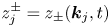 $z_j^\pm =z_\pm (\boldsymbol {k}_j,t)$ and the expressions for
 $V^{(\,j)}_{1,2,3}$ for
 $j=1,\ldots , 10$ are listed in appendix C. Then, from (3.35a,b), Hamilton's equations given, with
 $H=H_2+H_3$, by
 \begin{equation} \frac{\partial z_\pm}{\partial t}=\textrm{i}\frac{\delta H}{\delta z_\pm^*}, \end{equation}
yield the evolution equations for  $z_\pm (\boldsymbol {k},t)$ that are explicitly written in (B 23).
The system given by (3.40) is an alternative to the second-order spectral model for ( $q_\pm$,
 $p_\pm$) given by (B 18)–(B 21) and is valid for both resonant and non-resonant interactions. While the original system of four equations given by (B 18)–(B 21) has been reduced to a system of two equations in (B 22)–(B 23), the number of degrees of freedom, or the number of real unknowns remains the same as there are no relationships between
 $z_\pm$ and their complex conjugates. Therefore,
 $z_\pm$ are defined in the whole
 $\boldsymbol {k}$-plane while
 $p_\pm$ and
 $q_\pm$ can be defined only in a half of the
 $\boldsymbol {k}$-plane as they are related to their complex conjugates, as shown in (3.32a,b). Nevertheless, to be shown in the followings, the system for
 $z_\pm$ is advantageous to study the resonant interactions between the surface and internal wave modes.
3.5. Reduced Hamiltonians for resonant triad interactions
To study the resonant triad interactions, it is convenient to find a reduced Hamiltonian from  $H_3$. We first write
 $z_\pm$ as
 \begin{equation} z_\pm(\boldsymbol{k},t)={\mathcal{Z}}_\pm (\boldsymbol{k},t) \, \textrm{e}^{\textrm{i} \omega_\pm t}, \end{equation}
where, due to nonlinearity,  ${\mathcal {Z}}_\pm$ are assumed to depend on time. When (3.41) is substituted into the expression for
 $H_3$ given by (3.39), the integrands of
 $H_3$ can be expressed in terms of products of
 ${\mathcal {Z}}_\pm$ multiplied by exponential functions oscillating in time with frequencies that are linear combinations of the three wave frequencies. While the integrands are rapidly oscillatory for non-resonant triads, those for resonant waves become independent of fast time as their exponents vanish under the resonance conditions. Therefore, for resonant triads,
 ${\mathcal {Z}}_\pm$ depend only on the slow time, or, specifically,
 $\epsilon t$. Then, the evolution of resonant triads can be described by the reduced Hamiltonian that is independent of fast time
 $t$. This approach, widely used for gravity and gravity-capillary waves (Zakharov Reference Zakharov1968; Mei, Stiassnie & Yue Reference Mei, Stiassnie and Yue2005; Chabane & Choi Reference Chabane and Choi2019), will be adopted here.
3.5.1. Type-A resonant triad interactions
For type-A resonant interactions, the reduced Hamiltonian  $\mathcal {H}_{A}$ can be identified as
 \begin{equation} \mathcal{H}_{A}=\iiint V^{(2)}_{1,2,3} \left ({ \mathcal{Z}^+_1}^* \mathcal{Z}_2^+ \mathcal{Z}^-_3 \,\textrm{e}^{-\textrm{i} \varDelta_{1,2,3} t} + \mathcal{Z}^+_1 {\mathcal{Z}^+_2}^* {\mathcal{Z}^-_3}^*\,\textrm{e}^{ \textrm{i} \varDelta_{1,2,3} t}\right ) \delta_{1-2-3} \, \textrm{d}{\boldsymbol{k}}_{1,2,3} , \end{equation}
where 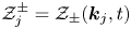 $\mathcal {Z}^\pm _j=\mathcal {Z}_\pm (\boldsymbol {k}_j,t)$, and
 $\varDelta _{1,2,3}=\omega _1^+-\omega _2^+-\omega _3^-=O(\epsilon )\ll 1$ has been assumed for near-resonant interactions. For exact resonances,
 $\varDelta _{1,2,3}=0$. This is the only integral that is independent of fast time under the type-A resonance frequency condition given by
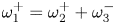 $\omega _1^{+}=\omega _2^{+} + \omega _3^{-}$ and depends only on slowly varying amplitude functions,
 $\mathcal {Z}^+_1$,
 $\mathcal {Z}^+_2$ and
 $\mathcal {Z}^-_3$. All other integrals rapidly oscillating in time have been neglected. For example, the terms proportional to
 $V^{(3)}_{1,2,3}$ and
 $V^{(8)}_{1,2,3}$ represent the interactions between two surface and one internal wave modes, but oscillate fast with the frequencies of
 $\pm (\omega _1^--\omega _2^+-\omega _3^+)$ and
 $\pm (\omega _1^+ +\omega _2^+ +\omega _3^-)$, respectively, that are non-vanishing. Therefore, they describe non-resonant interactions.
Then, from  ${\partial \mathcal {Z}_\pm /\partial t} =\textrm {i}(\delta \mathcal {H}_{A} /\delta \mathcal {Z}_\pm ^*)$, the slowly varying amplitude equations for
 $\mathcal {Z}_\pm$ are given by
 \begin{gather} \frac{\partial \mathcal{Z}_+}{\partial t} = \textrm{i} \iint \left (V^{(2)}_{0,1,2}\mathcal{Z}^+_1 \mathcal{Z}^-_2\,\textrm{e}^{-\textrm{i} \varDelta_{0,1,2} t} \delta_{0-1-2} + V^{(2)}_{2,0,1} {\mathcal{Z}^-_1}^* \mathcal{Z}^+_2 \,\textrm{e}^{\textrm{i} \varDelta_{2,0,1} t} \delta_{0+1-2}\right) \textrm{d}\boldsymbol{k}_{1,2} , \end{gather}
 \begin{gather}\frac{\partial \mathcal{Z}_- }{\partial t} = \textrm{i} \,\iint V^{(2)}_{1,2,0} \mathcal{Z}^+_1{\mathcal{Z}^+_2}^*\, \textrm{e}^{ \textrm{i} \varDelta_{1,2,0} t} \delta_{0-1+2} \, \textrm{d}\boldsymbol{k}_{1,2} . \end{gather}
It should be pointed out that, as  $\varDelta _{1,2,3}=\omega _1^+-\omega _2^+-\omega _3^-=O(\epsilon )\ll 1$, the integrations in (3.43) and (3.44) should be performed over the resonance region in the
 $(\boldsymbol {k}_1,\boldsymbol {k}_2)$-plane, where the resonance conditions (2.2) are approximately satisfied. As mentioned previously, the 1-D class-III resonance is the unidirectional limit of the type-A resonance and, therefore, the reduced Hamiltonian for the 1-D class-III resonance is still given by (3.42) once the integration is performed over a range of one-dimensional wavenumbers for which the 1-D class-III resonance is possible.
Under the exact resonance condition ( $\varDelta _{1,2,3}=0$), in addition to conservation of the reduced Hamiltonian
 $\mathcal {H}_{A}$, one can show that the system of (3.43) and (3.44) conserves the quantities
 \begin{equation} \frac{\textrm{d}}{\textrm{d} t}\int \left (\omega_+\vert \mathcal{Z}_+\vert^2+\omega_-\vert \mathcal{Z}_-\vert^2\right ) \textrm{d}\boldsymbol{k}=0,\quad \frac{\textrm{d}}{\textrm{d} t}\int \boldsymbol{k} \left (\vert \mathcal{Z}_+\vert^2+\vert \mathcal{Z}_-\vert^2\right ) \textrm{d}\boldsymbol{k}=0, \end{equation}
where the type-A resonance conditions given by (2.2) have been used.
For a single resonant triad satisfying the exact type-A resonance conditions (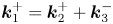 $\boldsymbol {k}_1^+=\boldsymbol {k}_2^++\boldsymbol {k}_3^-$ and
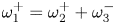 $\omega _1^+=\omega _2^++\omega _3^-$), a wave field is assumed to consist of two surface waves and one internal wave so that
 \begin{align} \mathcal{Z}_+(\boldsymbol{k},t)= \mathcal{Z}_1^+(t) \delta (\boldsymbol{k}-\boldsymbol{k}_1)+ \mathcal{Z}_2^+(t) \delta (\boldsymbol{k}-\boldsymbol{k}_2),\quad \mathcal{Z}_-(\boldsymbol{k},t)= \mathcal{Z}_3^-(t)\delta (\boldsymbol{k}-\boldsymbol{k}_3) . \end{align}
Then, the reduced Hamiltonian  $\mathcal {H}_{A}$ is given, from (3.42), by
 \begin{equation} \mathcal{H}_{A}= V^{(2)}_{1,2,3} ({\mathcal{Z}^+_1}^* \mathcal{Z}^+_2 \mathcal{Z}^-_3 + \mathcal{Z}^+_1 {\mathcal{Z}^+_2}^* {\mathcal{Z}^-_3}^*) , \end{equation}
from which the amplitude equations can be obtained,  $\dot {\mathcal {Z}}_j^{\pm } =\textrm {i}\delta \mathcal {H}_{A}/\delta {\mathcal {Z}_j^\pm }^*$, as
 \begin{equation} \dot{\mathcal{Z}}^+_1 = \textrm{i} V^{(2)}_{1,2,3}\mathcal{Z}^+_2 \mathcal{Z}^-_3 ,\quad \dot{\mathcal{Z}}^+_2 = \textrm{i} V^{(2)}_{1,2,3}\mathcal{Z}^+_1 {\mathcal{Z}^-_3}^* , \quad \dot{\mathcal{Z}}^-_3 = \textrm{i} V^{(2)}_{1,2,3} \mathcal{Z}^+_1 {\mathcal{Z}^+_2}^* , \end{equation}
where  $\dot {f}={\textrm {d} f}/{\textrm {d} t}$. Note that the coefficient
 $V^{(2)}_{1,2,3}$ can be made equal to one by rescaling
 $t$ if necessary. In addition to conservation of
 $\mathcal {H}_{A}$, it can be shown from (3.45a,b) and (3.46a,b) that the discrete system has the conservation laws
 \begin{align} \frac{\textrm{d}}{\textrm{d} t}\left (\omega_1^+\left\vert \mathcal{Z}^+_1 \right \vert^2+\omega_2^+\left\vert \mathcal{Z}^+_2\right \vert^2 +\omega_3^-\left\vert \mathcal{Z}^-_3\right \vert^2\right )=0,\enspace \frac{\textrm{d}}{\textrm{d} t}\left ( \boldsymbol{k}_1\left\vert \mathcal{Z}^+_1\right \vert +\boldsymbol{k}_2 \left\vert \mathcal{Z}^+_2\right \vert^2 +\boldsymbol{k}_3 \left\vert \mathcal{Z}^-_3\right\vert^2\right )=0, \end{align}
which can be shown, using (2.2), to be equivalent to
 \begin{equation} \frac{\textrm{d}}{\textrm{d} t}\left (\left\vert \mathcal{Z}^+_1 \right \vert^2+\left\vert \mathcal{Z}^+_2\right \vert^2\right )=0,\quad \frac{\textrm{d}}{\textrm{d} t}\left (\left\vert \mathcal{Z}^+_1 \right \vert^2+\left\vert \mathcal{Z}^-_3\right \vert^2\right )=0. \end{equation}
These are known as the Manley–Rowe relations (Manley & Rowe Reference Manley and Rowe1956).
To be shown later, in addition to an exact resonant triad  $(\boldsymbol {k}_1^+, \boldsymbol {k}_2^+, \boldsymbol {k}_3^-)$, a few additional surface wave modes can be excited through successive near-resonant interactions of type-A such that
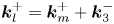 $\boldsymbol {k}_l^+=\boldsymbol {k}_m^++\boldsymbol {k}_3^-$ and
 $\omega _l^+=\omega _m^+ +\omega _3^-+\varDelta _{l,m,3}$ with
 $\vert \varDelta _{l,m,3}\vert \ll 1$. In such cases, the complex amplitude of the surface wave
 $\mathcal {Z}_+$ should be expressed as
 \begin{equation} \mathcal{Z}_+(\boldsymbol{k},t)= \mathcal{Z}_1^+(t) \delta (\boldsymbol{k}-\boldsymbol{k}_1^+)+ \mathcal{Z}_2^+(t) \delta (\boldsymbol{k}-\boldsymbol{k}_2^+) + \sum_{j=4}^{2(N+1)} \mathcal{Z}_{j}^+(t) \delta (\boldsymbol{k}-\boldsymbol{k}_{j}^+), \end{equation}
where  $N$ is a positive integer with
 $2N-1$ being the number of near-resonant triads and
 \begin{equation} \boldsymbol{k}_4^+=\boldsymbol{k}_1^++\boldsymbol{k}_3^-,\quad \boldsymbol{k}_{2n+1}^+=\boldsymbol{k}_1^+ - n\boldsymbol{k}_3^-, \quad \boldsymbol{k}_{2(n+1)}^+=\boldsymbol{k}_1^+ + n\boldsymbol{k}_3^-,\quad n\geqslant 2. \end{equation}
In (3.51),  $\mathcal {Z}_j^+$
 $(\,j \geqslant 4)$ represent the complex amplitudes of the successive near-resonant triads. For example, for
 $N=3$, from (3.43) and (3.44), the amplitude equations can be found as
 \begin{align} {\dot{\mathcal{Z}}}^+_1 &= \textrm{i} \left (V^{(2)}_{1,2,3}\mathcal{Z}^+_{2} \mathcal{Z}^-_3\,\textrm{e}^{-\textrm{i} \varDelta_{1,{2},3} t} + V^{(2)}_{4,1,3}\mathcal{Z}^+_{4} {\mathcal{Z}^-_3}^*\,\textrm{e}^{\textrm{i} \varDelta_{{4},1,3} t}\right ) , \end{align}
 \begin{align}\dot{\mathcal{Z}}^+_{2}&=\textrm{i} \left (V^{(2)}_{1,2,3}\mathcal{Z}^+_1 {\mathcal{Z}^-_3}^*\,\textrm{e}^{\textrm{i} \varDelta_{1,2,3} t} + V^{(2)}_{2,5,3}\mathcal{Z}^+_{5} {\mathcal{Z}^-_3}\,\textrm{e}^{-\textrm{i} \varDelta_{2,5,3} t}\right ) , \end{align}
 \begin{align} \dot{\mathcal{Z}}^-_3 &= \textrm{i} \left (V^{(2)}_{1,2,3} \mathcal{Z}^+_1 {\mathcal{Z}^+_{2}}^*\,\textrm{e}^{\textrm{i} \varDelta_{1,2,3} t} + V^{(2)}_{4,1,3} {\mathcal{Z}^+_1}^* {\mathcal{Z}^+_{4}}\,\textrm{e}^{\textrm{i} \varDelta_{{4,1,3} t}} \right. \nonumber\\ &\quad +V^{(2)}_{2,5,3} \mathcal{Z}^+_{2} {\mathcal{Z}^+_{5}}^*\,\textrm{e}^{\textrm{i} \varDelta_{2,5,3} t} + V^{(2)}_{6,4,3} {\mathcal{Z}^+_{4}}^* {\mathcal{Z}^+_{6}}\,\textrm{e}^{\textrm{i} \varDelta_{6,4,3} t} \nonumber\\ & \quad\left. +V^{(2)}_{5,7,3} \mathcal{Z}^+_{5} {\mathcal{Z}^+_{7}}^*\,\textrm{e}^{\textrm{i} \varDelta_{5,7,3} t} + V^{(2)}_{8,6,3} {\mathcal{Z}^+_{6}}^* {\mathcal{Z}^+_{8}}\,\textrm{e}^{\textrm{i} \varDelta_{8,6,3} t} \right ), \end{align}
 \begin{align} \dot{\mathcal{Z}}^+_{4}&= \textrm{i} \left (V^{(2)}_{4,1,3}\mathcal{Z}^+_1 {\mathcal{Z}^-_3}\,\textrm{e}^{-\textrm{i} \varDelta_{4,1,3} t} +V^{(2)}_{6,4,3}\mathcal{Z}^+_{6} {\mathcal{Z}^-_3}^*\,\textrm{e}^{\textrm{i} \varDelta_{6,4,3} t} \right ) , \end{align}
 \begin{align}\dot{\mathcal{Z}}^+_{5}&=\textrm{i} \left (V^{(2)}_{2,5,3}\mathcal{Z}^+_{2} {\mathcal{Z}^-_3}^*\,\textrm{e}^{\textrm{i} \varDelta_{2,5,3} t} + V^{(2)}_{5,7,3}\mathcal{Z}^+_{7} {\mathcal{Z}^-_3}\,\textrm{e}^{-\textrm{i} \varDelta_{5,7,3} t}\right ) , \end{align}
 \begin{align}\dot{\mathcal{Z}}^+_{6}&=\textrm{i} \left (V^{(2)}_{6,4,3}\mathcal{Z}^+_{4} {\mathcal{Z}^-_3}\,\textrm{e}^{-\textrm{i} \varDelta_{{6},{4},3} t} + V^{(2)}_{8,6,3}\mathcal{Z}^+_{8} {\mathcal{Z}^-_3}^*\,\textrm{e}^{\textrm{i} \varDelta_{8,6,3} t}\right ) , \end{align}
 \begin{align}\dot{\mathcal{Z}}^+_{7}&=\textrm{i} V^{(2)}_{5,7,3}\mathcal{Z}^+_{5} {\mathcal{Z}^-_3}^*\,\textrm{e}^{\textrm{i} \varDelta_{5,7,3} t}, \quad \dot{\mathcal{Z}}^+_{8}=\textrm{i} V^{(2)}_{8,6,3}\mathcal{Z}^+_{6} {\mathcal{Z}^-_3} \,\textrm{e}^{-\textrm{i} \varDelta_{8,6,3} t}. \end{align}
If no successive near-resonant interactions occur, (3.53)–(3.55) with  $\mathcal {Z}_j=0$
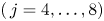 $(\,j=4, \ldots ,8)$ can be reduced to (3.48a–c). For
 $N=1$, the amplitude equations are given by (3.53)–(3.56) with
 $\mathcal {Z}_j=0$
 $(\,j=5,6,7,8)$ and, for
 $N=2$, by (3.53)–(3.58) with
 $\mathcal {Z}_7=\mathcal {Z}_8=0$.
3.5.2. Type-B resonant triad interactions
For type-B resonant interactions between one surface wave and two internal waves, the reduced Hamiltonian  $\mathcal {H}_{B}$ can be found as
 \begin{equation} \mathcal{H}_{B}=\iiint V^{(5)}_{1,2,3} \left ({\mathcal{Z}^+_1}^* \mathcal{Z}^-_2 \mathcal{Z}^-_3 \,\textrm{e}^{-\textrm{i} \varDelta_{1,2,3} t} + \mathcal{Z}^+_1 {\mathcal{Z}^-_2}^* {\mathcal{Z}^-_3}^* \,\textrm{e}^{ \textrm{i} \varDelta_{1,2,3} t} \right ) \delta_{1-2-3}\, \textrm{d}{\boldsymbol{k}}_{1,2,3} , \end{equation}
from which the amplitude equations for  $\mathcal {Z}_\pm$ are given, using
 ${\partial \mathcal {Z}_\pm /\partial t} =\textrm {i}(\delta \mathcal {H}_{B}/\delta \mathcal {Z}_\pm ^*)$, by
 \begin{gather} \frac{\partial \mathcal{Z}_+}{\partial t} = \textrm{i} \iint V^{(5)}_{0,1,2} \mathcal{Z}^-_1 \mathcal{Z}^-_2\, \textrm{e}^{-\textrm{i} \varDelta_{0,1,2} t}\delta_{0-1-2}\, \textrm{d}\boldsymbol{k}_{1,2} , \end{gather}
 \begin{gather}\frac{\partial \mathcal{Z}_-}{\partial t} = \textrm{i} \iint \left (V^{(5)}_{1,0,2}+ V^{(5)}_{1,2,0} \right ) \mathcal{Z}^+_1 {\mathcal{Z}^-_2}^*\,\textrm{e}^{\textrm{i} \varDelta_{1,0,2} t} \delta_{0-1+2} \,\textrm{d}\boldsymbol{k}_{1,2} . \end{gather}
For the type-B resonance,  $\varDelta _{1,2,3}$ is defined as
 $\varDelta _{1,2,3}=\omega _1^+-\omega _2^- - \omega _3^-$. Under the exact resonance condition (
 $\varDelta _{1,2,3}=0$), the system for the type-B resonance given by (3.61) and (3.62) also satisfies the conservations laws given by (3.45a,b). Similarly to the type-A resonance, the terms proportional to
 $V^{(4)}_{1,2,3}$ and
 $V^{(9)}_{1,2,3}$ describe non-resonant interactions between one surface and two internal wave modes.
For a single triad satisfying the exact type-B resonance conditions (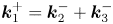 $\boldsymbol {k}_1^+=\boldsymbol {k}_2^-+\boldsymbol {k}_3^-$ and
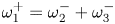 $\omega _1^{+}=\omega _2^{-}+\omega _3^{-}$),
 $\mathcal {Z}_\pm$ can be written as
 \begin{align} \mathcal{Z}_+(\boldsymbol{k},t)= \mathcal{Z}_1^+(t) \delta (\boldsymbol{k}-\boldsymbol{k}_1^+),\quad \mathcal{Z}_-(\boldsymbol{k},t)= \mathcal{Z}_2^-(t) \delta (\boldsymbol{k}-\boldsymbol{k}_2^-)+\mathcal{Z}_3^-(t)\delta (\boldsymbol{k}-\boldsymbol{k}_3^-). \end{align}
Then the amplitude equations can be found, from  ${\dot {\mathcal {Z}}_j^\pm } =\textrm {i}\delta \mathcal {H}_{B} /\delta {\mathcal {Z}_j^\pm }^*$, as
 \begin{equation} \dot{\mathcal{Z}}^+_1 = \textrm{i} \left (V^{(5)}_{1,2,3}+V^{(5)}_{1,3,2}\right )\mathcal{Z}^-_2 \mathcal{Z}^-_3, \quad \dot{\mathcal{Z}}^-_{2,3} = \textrm{i} \left (V^{(5)}_{1,2,3}+V^{(5)}_{1,3,2}\right )\mathcal{Z}^+_1 {\mathcal{Z}^-_{3,2}}^* . \end{equation}
Similarly to the type-A resonance, under the exact resonance conditions given by (2.3), it can be shown the system obeys the conservation laws
 \begin{align} \frac{\textrm{d}}{\textrm{d} t}\left (\omega_1^+\left\vert \mathcal{Z}^+_1 \right \vert^2+\omega_2^-\left\vert \mathcal{Z}^-_2\right \vert^2 +\omega_3^-\left\vert \mathcal{Z}^-_3\right \vert^2\right )=0,\enspace \frac{\textrm{d}}{ \textrm{d} t}\left ( \boldsymbol{k}_1\left\vert \mathcal{Z}^+_1\right \vert +\boldsymbol{k}_2 \left\vert \mathcal{Z}^-_2\right \vert^2 +\boldsymbol{k}_3 \left\vert \mathcal{Z}^-_3\right\vert^2\right )=0, \end{align}
which yield the Manley–Rowe relations given by (3.50a,b) with replacing  $\mathcal {Z}_2^+(t)$ by
 $\mathcal {Z}_2^-(t)$.
For near-resonant interactions, the right-hand sides of the amplitude (3.64a,b) need to be multiplied by  $\exp (-\textrm {i}\varDelta _{1,2,3}t)$ and
 $\exp (\textrm {i}\varDelta _{1,2,3}t)$, respectively. Unlike the type-A resonance, from the type-B resonance conditions (2.15a,b), one can note that successive near-resonant interactions are unlikely to occur with
 $\varOmega _+>\varOmega _-$.
4. Numerical solutions for 2-D resonant triad interactions
4.1. Numerical method for the Hamiltonian system
To solve numerically the explicit Hamiltonian system (3.3)–(3.6) after it is non-dimensionalized with respect to  $h_1$ and
 $g$, we adopt a pseudo-spectral method based on the fast Fourier transform algorithm similar to that used in Taklo & Choi (Reference Taklo and Choi2020) for 1-D waves. While the detailed description and discussion about the numerical scheme and its accuracy can be found in Taklo & Choi (Reference Taklo and Choi2020), they are summarized as follows. We let
 $L_x$ and
 $L_y$ be the lengths in the
 $x$- and
 $y$-directions of the computational domain. The number of Fourier modes is
 $N_x \times N_y$, where
 $N_x$ and
 $N_y$ are the numbers of grid points along the
 $x$- and
 $y$-directions, respectively. Typically we use 16 grid points per wavelength. The linear integral operators
 $\varGamma _{ij}$ in the Hamiltonian system are evaluated in Fourier space using (3.10). The smallest wavenumbers resolved in Fourier space are given by
 ${\rm \Delta} K_x=2{\rm \pi} /L_x$ and
 ${\rm \Delta} K_y=2{\rm \pi} /L_y$. Once the right-hand sides of the Hamiltonian system are evaluated using the pseudo-spectral method, the system is integrated in time using a fourth-order Runge–Kutta scheme with time step
 ${\rm \Delta} t$. To avoid aliasing errors resulting from the use of truncated Fourier series, a low-pass filter is applied to eliminate one-third of the highest wavenumber modes.
The pseudo-spectral model requires periodic boundary conditions. Then, the  $x$- and
 $y$-components of the wavenumber vector (
 ${K}_x$ and
 ${K}_y$) need to be integer multiples of each other so that the waves whose wavelengths are given by
 $\lambda _x=2{\rm \pi} /K_x$ and
 $\lambda _y=2{\rm \pi} /K_y$ are periodic within the computational domain. Under this restriction, the
 $x$-components of the wavenumber vectors for two waves in a resonant triad, say
 ${K_l}_x$ and
 ${K_n}_x$, are fixed with
 ${K_l}_x=M{K_n}_x$, where an integer
 $M$ and
 ${K_n}_x$ are chosen as two free parameters in the problem. Considering that we have chosen
 ${K_1}_y=0$, the resonance condition for the wavenumber vectors given by (2.5) requires
 ${K_1}_x={K_2}_x+{K_3}_x$ and
 ${K_2}_y={K_3}_y$. Then the only unknown is
 ${K_2}_y$, which can be determined by the frequency condition (2.6).
The lengths of the total computational domain for the Hamiltonian system are chosen to be 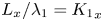 $L_x/\lambda _1={K_1}_x$ and
 $L_y/\lambda _1=2{K_1}_x/\vert {K_2}_y\vert$, where
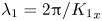 $\lambda _1=2{\rm \pi} /{K_1}_x$.
To initialize  $\zeta _{1,2}$ and
 $\varPsi _{1,2}$ for the explicit Hamiltonian system (3.3)–(3.6), their Fourier coefficients
 $a_\pm$ and
 $b_\pm$ can be prescribed. For example, for the surface (or internal) wave mode,
 $a_+$ (or
 $a_-$) is given and the remaining variables are computed using their linear relationships given by (A 15) and (A 16). Then, after assuming that only two wave modes in a resonant triad initially have non-zero amplitudes, we monitor the growth of the third mode and the subsequent interaction among the three modes.
4.2. Link to the amplitude equations
To solve the amplitude equations, one should initialize  $\mathcal {Z}_\pm$ in a way consistent with the initial conditions for the Hamiltonian system and transform the solutions of the amplitude equations back to the original physical variables for the Hamiltonian system. In other words,
 $\mathcal {Z}_\pm$ need to be related to
 $a_\pm$ and
 $b_\pm$.
From (3.31a,b) and (3.37a,b), for a pure surface wave mode  $(q_-=p_-=0)$,
 $a_\pm$ and
 $b_\pm$ can be expressed, in terms of
 $q_+$ and
 $p_+$, as
 \begin{equation} a_\pm (\boldsymbol{K},t)=Q^{(m,1)}q_+,\quad b_\pm (\boldsymbol{K},t)=P^{(m,1)}p_+, \end{equation}
where  $m=1$ for
 $a_+$ and
 $b_+$ and
 $m=2$ for
 $a_-$ and
 $b_-$. Note that
 $a_+$ and
 $a_-$ are the Fourier coefficients of the surface and interface displacements, respectively, induced by the surface wave motion. On the other hand, for a pure internal wave mode
 $(q_+=p_+=0)$, the expressions for
 $a_\pm$ and
 $b_\pm$ are given, in terms of
 $q_-$ and
 $p_-$, by
 \begin{equation} a_\pm (\boldsymbol{K},t) = Q^{(m,2)} q_-,\quad b_\pm (\boldsymbol{K},t) = P^{(m,2)} p_-. \end{equation}
For small amplitude waves, when the system given by (B 18)–(B 21) is linearized, the relationships between  $p_\pm$ and
 $q_\pm$ can be found as
 \begin{equation} p_\pm=\textrm{i} \varOmega_\pm q_\pm, \end{equation}
which can be substituted into (3.36) to find the expressions for  $z_\pm$ as
 \begin{equation} z_\pm=\sqrt{2\varOmega_\pm}\,q_\pm=-\textrm{i} \sqrt{2/\varOmega_\pm} \,p_\pm. \end{equation}
Then, from (4.1a,b)–(4.2a,b) and (4.4),  $a_\pm$ and
 $b_\pm$ can be related to
 $z_\pm$, for a pure surface wave mode, as
 \begin{equation} a_\pm(\boldsymbol{K},t) \approx \frac{1}{\sqrt{2\varOmega_+}}\,Q^{(m,1)} z_+(\boldsymbol{K},t),\quad b_\pm(\boldsymbol{K},t) \approx \textrm{i} \sqrt{\frac{\varOmega_+}{2}}\,P^{(m,1)}z_+(\boldsymbol{K},t), \end{equation}
and, for a pure internal wave mode, as
 \begin{equation} a_\pm (\boldsymbol{K},t) \approx \frac{1}{\sqrt{2\varOmega_-}}\, Q^{(m,2)} z_-(\boldsymbol{K},t),\quad b_\pm (\boldsymbol{K},t) \approx \textrm{i} \sqrt{\frac{\varOmega_-}{2}}\,P^{(m,2)}z_-(\boldsymbol{K},t), \end{equation}
where, once again,  $m=1$ for
 $a_+$ and
 $b_+$ and
 $m=2$ for
 $a_-$ and
 $b_-$. Equations (4.5a,b) and (4.6a,b) provide, under the small amplitude assumption, the leading-order relationships of
 $a_\pm$ and
 $b_\pm$ with
 $z_\pm (\boldsymbol {k},t)$ and, therefore,
 $\mathcal {Z}_\pm (\boldsymbol {k},t)$. These are then used to initialize the amplitude equations to be consistent with the Hamiltonian system and to compare the numerical solutions of the two models. In particular, the real amplitudes
 $A_+=2\vert a_+\vert$ and
 $A_-=2\vert a_-\vert$ for the surface and internal wave modes, respectively, are monitored for the explicit Hamiltonian system and can be related to
 $\mathcal {Z}_\pm$ as
 \begin{equation} A_+ (\boldsymbol{K},t) = \sqrt{\frac{2}{\varOmega_+}}\left \vert Q^{(1,1)}\right \vert \left\vert \mathcal{Z}_+ (\boldsymbol{K},t) \right \vert ,\quad A_- (\boldsymbol{K},t) = \sqrt{\frac{2}{\varOmega_-}}\left \vert Q^{(2,2)}\right \vert \left\vert \mathcal{Z}_- (\boldsymbol{K},t) \right \vert , \end{equation}
where, from (3.41),  $\vert z_\pm \vert =\vert \mathcal {Z}_\pm \vert$ have been used.
4.3. Numerical results
We numerically study five different 2-D resonant triad interactions: three cases for type A and two for type B. Both the Hamiltonian system and the amplitude equations described in §§ 3.1 and 3.5, respectively, are solved numerically and their solutions are compared. As presented later, the plots for the surface and interface displacements show the whole computational domain.
For the weakly nonlinear assumption for these models to be valid, the initial wave steepnesses defined by  $K_jA_j$ should be small. In addition, the dimensionless real wave amplitudes
 $A_j$ introduced in (4.7a,b) are assumed to be small, which means the wave amplitudes are small compared with the upper layer thickness
 $h_1$. This additional assumption is crucial particularly for small
 $K_j$ for which higher-order nonlinearities for long waves missing in the second-order model need to be taken into account. Here we choose both
 $K_jA_j$ and
 $A_j$ to be
 $O(10^{-2})$. Table 1 summarizes the dimensionless wave parameters of resonant triads used for computations, including the wavenumbers, wave frequencies and propagation angles along with the coefficients of the amplitude equations.
Dimensionless physical parameters for numerical solutions of the Hamiltonian system and the amplitude equations for type-A (A1, A2, A3) and type-B (B1, B2) resonances. Here  $\boldsymbol {K}_j^\pm =\boldsymbol {k}_j^\pm h_1$,
 $\varOmega _j^\pm =\omega _j^\pm /(g/h_1)^{1/2}$ and
 $A_j^\pm =2\vert a_j^\pm \vert /h_1$. The depth ratio and the propagation angle of
 $\boldsymbol {K}_1$ are fixed to be
 $h_2/h_1$=4 and
 $\theta _1=0$, respectively.

4.3.1. Type-A resonant interactions
(i) Case A1. As discussed in § 2.2, the type-A resonance is the resonant interaction between two surface waves and one internal wave. The first case considered here is when the two surface waves with  $\boldsymbol {K}_1^+=(2,0)$ and
 $\boldsymbol {K}_2^+=(0,1.012)$ propagate perpendicularly to each other. The density and depth ratios are chosen to be
 $\rho _2/\rho _1=1.163$ and
 $h_2/ h_1=4$. While the initial wave steepnesses are
 $K_1^+A_1^+=K_2^+A_2^+=0.01$, note that the wave amplitudes relative to
 $h_1$ are given by
 $A_1^+ =0.005$ and
 $A_2^+\approx 0.01$ so that the
 $K_2^+$ wave propagating in the
 $y$-direction has a larger amplitude. Through the resonant triad interaction, an internal wave with
 $\boldsymbol {K}_3^-=\boldsymbol {K}_1^+ - \boldsymbol {K}_2^+=(2,-1.012)$ is expected to be excited.
Figure 8 shows the numerical solutions of the Hamiltonian system for the surface and interface displacements,  $\zeta _1$ and
 $\zeta _2$, at
 $t/T_1=0$, 2700, 4200, where
 $T_1=2{\rm \pi} /\varOmega _1^+$ is the wave period of the
 $K_1^+$ wave. Initially the surface displacement is a linear combination of two orthogonal surface waves while the amplitude of the
 $K_3^-$ wave is zero. Note that the interface is slightly perturbed in figure 8(
 $b$) even in the absence of the internal wave mode and displays the surface wave mode contribution to the interface displacement
 $\zeta _2$. The ratio of
 $\zeta _2$ to
 $\zeta _1$ for the surface wave mode is given by
 $\zeta _2/\zeta _1=Q^{(2,1)}/Q^{(1,1)}\approx 0.363$ for
 $K=K_2^+$. The excitation of the
 $K_3^-$ wave with
 $\theta _3^-\approx -26.84^{\circ }$ can be clearly seen in figure 8(
 $d$).
Numerical solutions of the Hamiltonian system given by (3.3)–(3.6) for case A1: (a,c,e) surface displacement  $\zeta _1$ and (b,d,f) interface displacement
 $\zeta _2$ at (a,b)
 $t/T_1=0$, (c,d)
 $t/T_1=2700$ and (e,f)
 $t/T_1=4200$. The initial wave steepnesses are
 $K_1^+A_1^+=K_2^+A_2^+=0.01$, and
 $K_3^-A_3^-=0$ with
 $K_1^+=2$,
 $K_2^+=1.012$ and
 $K_3^-=2.241$. The angles of wave propagation are
 $\theta _1^+=0$,
 $\theta _2^+=90^{\circ }$,
 $\theta _3^-\approx -26.84^{\circ }$. The displacements are normalized by the initial amplitude of
 $A_2^+$, or
 $A_2^+(0)$.

Figure 9 shows the comparison for the wave amplitudes ( $A_1^+, A_2^+, A_3^-$) between the Hamiltonian system and the amplitude equations for a single triad given by (3.48a–c). For the Hamiltonian system, the amplitudes
 $A_1^+$ and
 $A_2^+$ are computed from the Fourier coefficients of
 $\zeta _1$ for
 $\boldsymbol {K}=\boldsymbol {K}_1^+$ and
 $\boldsymbol {K}_2^+\,(=\boldsymbol {K}_1^+-\boldsymbol {K}_3^-)$, respectively, while
 $A_3^-$ is computed from the Fourier coefficient of
 $\zeta _2$ for
 $\boldsymbol {K}=\boldsymbol {K}_3^-$. The solutions of the amplitude equations for
 $\mathcal {Z}_j^\pm$ are transformed to the real amplitudes
 $A_j^\pm$, from (4.7a,b), as
 \begin{equation} A_j^+ = \sqrt{\frac{2}{\varOmega_j^+}}\left \vert Q_j^{(1,1)}\right \vert \left\vert \mathcal{Z}_j^+ \right \vert\quad \mbox{for } j=1,2,\quad A_3^- = \sqrt{\frac{2}{\varOmega_3^-}}\left \vert Q_3^{(2,2)}\right \vert \left\vert \mathcal{Z}_3^- \right \vert , \end{equation}
where  $Q_{1,2}^{(1,1)}=Q^{(1,1)}(K_{1,2}^+)$ and
 $Q_3^{(2,2)}=Q^{(2,2)}(K_3^-)$. The coefficient
 $V^{(2)}_{1,2,3}$ for the amplitude equations is listed in table 1. As shown in figure 9, some minor differences are observed and increase with time. Considering the wave steepness
 $\epsilon =O(10^{-2})$, the total computational time is
 $t/T_1=12\,000=O(\epsilon ^{-2})$ and is much greater than the time scale for the second-order theory, which is
 $O(\epsilon ^{-1})$. Nevertheless, it can be noticed that the single triad reasonably well describe the surface and interface motions, or the evolutions of
 $\zeta _1$ and
 $\zeta _2$. The numerical solutions of the explicit Hamiltonian system show that the triad exchanges energy quasi-periodically in time and the recurrence period is close to what the amplitude equations predict. The numerical results clearly demonstrate that the resonant triad interaction is a mechanism for the generation of an initially absent internal wave from two surface waves propagating with an angle.
Time evolution of the wave amplitudes for case A1. The numerical solutions of the Hamiltonian system given by (3.3)–(3.6) (lines) compared with those of the amplitude equations (symbols) given by (3.48a–c). For the Hamiltonian system, the amplitudes  $A_1^+$ (solid, open circles) and
 $A_2^+$ (dashed, open squares) are computed from the Fourier coefficients of
 $\zeta _1$ for
 $\boldsymbol {K}=\boldsymbol {K}_1^+$ and
 $\boldsymbol {K}_2^+(=\boldsymbol {K}_1^+-\boldsymbol {K}_3^-)$, respectively, while
 $A_3^-$ (dotted, filled squares) is computed from the Fourier coefficient of
 $\zeta _2$ for
 $\boldsymbol {K}=\boldsymbol {K}_3^-$. Note that the amplitudes are normalized by
 $A_2^+(0)$.

(ii) Case A2. Next, for the same density and depth ratios, we consider the case, where one surface wave with  $\boldsymbol {K}_1^+=(4,0)$ and one internal wave with
 $\boldsymbol {K}_3^-=(1,-0.331)$ initially propagate with an angle
 $\theta _3^-=-18.33^{\circ }$. Their initial wave steepnesses are
 $K_1^+A_1^+=K_3^-A_3^-=0.01$. From the type-A resonance conditions given by (2.11a,b), one expects a surface wave with
 $\boldsymbol {K}_2^+=\boldsymbol {K}_1^+-\boldsymbol {K}_3^-=(3, 0.331)$ to be excited. Even though the resonance condition is not exactly satisfied, another resonant triad
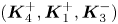 $(\boldsymbol {K}_4^+, \boldsymbol {K}_1^+,\boldsymbol {K}_3^-)$ is also possible with
 $\boldsymbol {K}_4^+=\boldsymbol {K}_1^+ +\boldsymbol {K}_3^-=(5,-0.331)$. As the frequency is slightly detuned, or
 $\varDelta _{4,1,3}=\varOmega _4^+-\varOmega _1^+-\varOmega _3^-=0.0242 \ll 1$, the near-resonant triad is expected to exchange energy with the primary triad
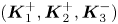 $(\boldsymbol {K}_1^+, \boldsymbol {K}_2^+,\boldsymbol {K}_3^-)$. Therefore, the evolution of the
 $K_4^-$ wave cannot be neglected and needs to be included in the amplitude equations. When the surface wave is written as (3.51) with
 $N=1$, the coupled amplitude equations for the two triads (or
 $\mathcal {Z}_j$ for
 $j=1,2,3,4$) are given by (3.53)–(3.56) with
 $\mathcal {Z}_l=0$ for
 $l=5,6,7,8$.
The results are shown in figures 10 and 11. Initially, a surface wave propagates in the positive  $x$-direction while an internal wave propagates with
 $\theta _3^-=-18.33^{\circ }$, as shown in figure 10(a,b). Note that the initial internal wave amplitude
 $A_3^-$ is approximately four times greater than
 $A_1^+$ and the scales in the
 $x$- and
 $y$-directions in the plot are different. At
 $t/T=150$, the
 $K_2^+$ wave with
 $\theta _2^+=6.30^{\circ }$ that is initially absent is clearly generated on the surface, as can be seen in figure 10
 $(c)$, although the amplitude of the interface displacement shown in figure 10(b,d,f) remains almost unchanged.
Numerical solutions of the Hamiltonian system given by (3.3)–(3.6) for case A2: (a,c,e) surface displacement  $\zeta _1$ and (b,d,f) interface displacement
 $\zeta _2$ at (a,b)
 $t/T_1=0$, (c,d)
 $t/T_1=150$ and (e,f)
 $t/T_1=250$. The initial wave steepnesses are
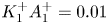 $K_1^+A_1^+=0.01$,
 $K_2^+A_2^+=K_4^+A_4^+=0$ and
 $K_3^-A_3^-=0.01$ with
 $K_1^+=4$,
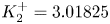 $K_2^+=3.01825$,
 $K_3^-=1.05348$,
 $K_4^+=5.011$. The angles of wave propagation are
 $\theta _1^+=0$,
 $\theta _2^+\approx 6.30^{\circ }$,
 $\theta _3^-\approx -18.33^{\circ }$,
 $\theta _4^+\approx -3.79^{\circ }$. The displacements are normalized by
 $A_3^-(0)$.

Time evolution of the wave amplitudes for case A2. The numerical solutions of the Hamiltonian system given by (3.3)–(3.6) (lines) are compared with those of the amplitude equations (symbols) for two triads including a near-resonant triad ( $N=1$). For the Hamiltonian system, the amplitudes
 $A_1^+$ (solid, open circles),
 $A_2^+$ (dashed, open squares) and
 $A_4^+$ (dash–dotted, filled squares) are computed from the Fourier coefficients of
 $\zeta _1$ for
 $\boldsymbol {K}=\boldsymbol {K}_1^+$,
 $\boldsymbol {K}_2^+(=\boldsymbol {K}_1^+-\boldsymbol {K}_3^-)$ and
 $\boldsymbol {K}_4^+(=\boldsymbol {K}_1^++\boldsymbol {K}_3^-)$, respectively, while
 $A_3^-$ (dotted, dots) is computed from the Fourier coefficient of
 $\zeta _2$ for
 $\boldsymbol {K}=\boldsymbol {K}_3^-$. Note that the wave amplitudes are normalized by
 $A_3^-(0)$.

While the  $K_4^+$ wave with
 $\theta _4^+=3.79^{\circ }$ should be excited, it is a little difficult to identify in figure 10
 $(c)$ although it is visible in figure 10
 $(e)$. As shown in figure 11, the
 $K_4^+$ wave is surely excited, but its amplitude remains smaller than that of the
 $K_1^+$ or
 $K_2^+$ wave. Nevertheless, the second resonant triad interaction must be included to predict the detailed evolution of the primary resonant triad.
(iii) Case A3. Surface signatures of large amplitude long internal waves have been of interest for their applications to remote sensing and have been attributed to near-resonant interactions between surface and internal waves. In particular, when a group of short surface waves propagates with its group velocity that is close to the phase velocity of a long internal wave, the short surface waves are greatly modulated. Once their amplitudes become large enough, the surface waves start to exchange energy with each other. This process has been studied for 1-D waves using the Hamiltonian system in Taklo & Choi (Reference Taklo and Choi2020). Here, we study this process for 2-D waves under a realistic oceanic condition with  $\rho _2/\rho _1=1.01$ and
 $h_2/h_1=4$.
Similarly to case A2, the initial wave field consists of one surface wave with 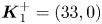 $\boldsymbol {K}_1^+=(33,0)$ and one internal wave with
 $\boldsymbol {K}_3^-=(1,-1.168)$, and the angle between the two wave directions is
 $\theta _3=-49.42^{\circ }$. As pointed out previously in § 2.2, when a 2-D resonant triad inside the type-A resonance region is located close to the 1-D class-III resonance curve, the surface wavenumbers are much greater than the internal wavenumber particularly when the density ratio is close to 1. For case A3, the ratio between the surface and internal wavenumbers is given by
 $K_1^+/K_3^-= 33/1.537\approx 21.47$. While the initial steepnesses for the two waves are the same (
 $K_1^+A_1^+=K_3^-A_3^-=0.01$), the internal wave amplitude is approximately 20 times greater than the surface wave amplitude. As shown for case A2, we expect the interactions between the two primary resonant triads: (
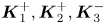 $\boldsymbol {K}_1^+,\boldsymbol {K}_2^+,\boldsymbol {K}_3^-$) and (
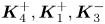 $\boldsymbol {K}_4^+,\boldsymbol {K}_1^+,\boldsymbol {K}_3^-$), where
 $\boldsymbol {K}_2^+=\boldsymbol {K}_1^+ - \boldsymbol {K}_3^-$ and
 $\boldsymbol {K}_4^+=\boldsymbol {K}_1^++\boldsymbol {K}_3^-$. From our choice, the first is the exact resonant triad while the second is a near-resonant triad with the detuning parameter
 $\varDelta _{4,1,3}=\varOmega _4^+-\varOmega _1^+-\varOmega _3^-=0.0242$, as listed in table 2.
Dimensionless physical parameters for successive type-A resonant interactions. For case A2, a near-resonant triad satisfying  $\boldsymbol {K}_4^+=\boldsymbol {K}_1^+ + \boldsymbol {K}_3^-$ and
 $\varOmega _4^+=\varOmega _1^+ + \varOmega _3^-+\varDelta _{4,1,3}$ is considered. For case A3, included are four more additional triads:
 $(\boldsymbol {K}_2^+, \boldsymbol {K}_5^+,\boldsymbol {K}_3^-)$,
 $(\boldsymbol {K}_6^+, \boldsymbol {K}_4^+,\boldsymbol {K}_3^-)$,
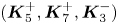 $(\boldsymbol {K}_5^+, \boldsymbol {K}_7^+,\boldsymbol {K}_3^-)$,
 $(\boldsymbol {K}_8^+, \boldsymbol {K}_6^+,\boldsymbol {K}_3^-)$. The initial amplitudes of all near-resonant triads are zero.

The numerical solutions of the Hamiltonian system for the surface and interface displacements are shown in figure 12. At  $t/T_1=400$ with
 $T_1=2{\rm \pi} /\varOmega _1^+$, one can notice that the interface changes little, but the top surface shows distinctive streaks that are almost aligned with the crestlines of the internal wave. These streaks are visible as the short surface wave with
 $K_1^+$ is modulated and its local amplitude over the internal wave crestlines increases. At
 $t/T_1=800$, other surface modes are excited through successive resonant interactions and each streak is distorted.
Numerical solutions of the Hamiltonian system given by (3.3)–(3.6) for case A3: (a,c,e) surface displacement intensities  $\zeta _1$ and (b,d,f) interface displacement intensities
 $\zeta _2$ at
 $(a,\!b)$
 $t/T_1=0$, (c,d)
 $t/T_1=400$, (e,f)
 $t/T_1=800$. The initial wave steepnesses are
 $K_1^+A_1^+=K_3^-A_3^-=0.01$ and
 $K_2^+A_2^+=0$ with
 $K_1^+=33$,
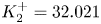 $K_2^+=32.021$ and
 $K_3^-=1.537$. The angles of wave propagation are
 $\theta _1^+=0$,
 $\theta _2^+\approx 2.09^{\circ }$ and
 $\theta _3^-\approx -49.42^{\circ }$. The displacements are normalized by
 $A_1^+(0)$.

Unlike case A2, successive near-resonant triad interactions can occur more easily as the density ratio is close to one (Alam Reference Alam2012; Taklo & Choi Reference Taklo and Choi2020). Through successive resonant interactions, one expects the generation of a number of surface wave modes, or sidebands, whose wavenumbers are given by  $\boldsymbol {K}_1^+\pm n\boldsymbol {K}_3^-$ (
 $n\geqslant 2$) with
 $K_3^-/K_1^+=0.0466 \ll 1$. Note that the
 $\boldsymbol {K}_1^+\pm \boldsymbol {K}_3^-$ waves belong to the two primary triads. Even for a finite value of
 $n$, the frequency resonance condition could still be approximately satisfied as the ratio
 $K_3^-/K_1^+$ is small. Therefore, to compare with the Hamiltonian system, one should include the amplitude equations for several triads that could be generated by the successive near-resonant interactions, as discussed in § 3.5.1.
As shown in figure 13( $a$), when the first successive triads with
 $\boldsymbol {K}_5^+=\boldsymbol {K}_1^+ - 2\boldsymbol {K}_3^-$ and
 $\boldsymbol {K}_6^+=\boldsymbol {K}_1^+ + 2\boldsymbol {K}_3^-$ are included, the numerical solutions of the amplitude equations given by (3.53)–(3.59a,b) with
 $N=2$ deviate from those of the Hamiltonian system as
 $t$ increases. When two more surface wave modes given by
 $\boldsymbol {K}_7^+=\boldsymbol {K}_1^+ - 3\boldsymbol {K}_3^-$ and
 $\boldsymbol {K}_8^+=\boldsymbol {K}_1^+ + 3\boldsymbol {K}_3^-$ are included, the two solutions agree well to
 $t/T_1=1200$, as can be seen in figure 13(
 $b$). Figure 14 shows the comparison between the two solutions for the amplitudes of the
 $K_j$ waves (
 $\,j=5,6,7,8$) excited by first and second successive resonant interactions. Their amplitudes are comparable with those of the two primary triads shown in figure 13(
 $b$). Therefore, for case A3, it can be concluded that at least the second successive resonant triads need to be included to correctly describe how the initial energy is spread to the sidebands. The parameters for all the surface wave modes excited by the successive interactions are listed in table 2. This demonstrates that, when the oceanic condition is met, the dynamics of near-resonant wave modes or sidebands are crucial to correctly describe the wave modulation on the top surface.
Time evolution of the wave amplitudes for case A3. The numerical solutions of the Hamiltonian system given by (3.3)–(3.6) (lines) are compared with those of the amplitude equations (symbols) given by (3.53)–(3.59a,b) with  $(a)$
 $N=2$ and
 $(b)$
 $N=3$. For the Hamiltonian system, the amplitudes
 $A_1^+$ (solid, open circles),
 $A_2^+$ (dashed, open squares) and
 $A_4^+$ (dash–dotted, filled squares) are computed from the Fourier coefficients of
 $\zeta _1$ for
 $\boldsymbol {K}=\boldsymbol {K}_1^+$,
 $\boldsymbol {K}_2^+=\boldsymbol {K}_1^+-\boldsymbol {K}_3^-$,
 $\boldsymbol {K}_4^+=\boldsymbol {K}_1^++\boldsymbol {K}_3^-$, respectively, and are normalized by
 $A_1^+(0)$. The internal wave amplitude
 $A_3^-$ changes little and is not shown here.

Time evolution of the wave amplitudes from successive near-resonant interactions for case A3. The numerical solutions of the Hamiltonian system given by (3.3)–(3.6) (lines) are compared with those of the amplitude equations (symbols) given by (3.53)–(3.59a,b) with  $N=3$. The amplitudes
 $A_5^+$ (solid, open circles),
 $A_6^+$ (dashed, open squares),
 $A_7^+$ (dash–dotted, filled squares) and
 $A_8^+$ (dotted, filled circles) are computed from the Fourier coefficients of
 $\zeta _1$ for
 $\boldsymbol {K}=\boldsymbol {K}_5^+=\boldsymbol {K}_1^+-2\boldsymbol {K}_3^-$,
 $\boldsymbol {K}_6^+=\boldsymbol {K}_1^++2\boldsymbol {K}_3^-$,
 $\boldsymbol {K}_7^+=\boldsymbol {K}_1^+-3\boldsymbol {K}_3^-$ and
 $\boldsymbol {K}_8^+=\boldsymbol {K}_1^++3\boldsymbol {K}_3^-$, respectively, and are normalized by
 $A_1^+(0)$.

4.3.2. Type-B resonant interactions
(i) Case B1. For the type-B resonance, we consider the interaction between one surface wave and two internal waves. As discussed in § 2.3, the resonance region in the  $(K_2^-, K_3^-)$-plane is symmetric about the straight line
 $K_2^-=K_3^-$, on which one can find symmetric resonant triads with
 $\theta _2^-=-\theta _3^-$. For the density and depth ratios given by
 $\rho _2/\rho _1=1.163$ and
 $h_2/h_1=4$, we assume that a surface wave with
 $\boldsymbol {K}_1^+=(2,0)$ and an internal wave with
 $\boldsymbol {K}_2^-=(1,6.567)$ that satisfy the symmetric resonance conditions so that another internal wave with
 $\boldsymbol {K}_3^-=(1,-6.567)$ is excited. As the propagation angles of the
 $K_2^-$ and
 $K_3^-$ waves are given by
 $\pm 81.34^{\circ }$, the two internal waves propagate almost in opposite directions and interact resonantly with the surface wave propagating in the positive
 $x$-direction that is almost perpendicular to the directions of the internal waves.
Figure 15 shows the numerical solutions of the Hamiltonian system at  $t/T_1=0$, 1200, 1700. The initial wave steepnesses of the
 $K_1^+$ and
 $K_2^-$ waves are chosen to be
 $K_1^+A_1^+=K_2^-A_2^-=0.025$ with
 $K_1^+=2$ and
 $K_2^-=6.643$. These steepnesses are slightly greater than those for other cases, but the greater initial wave amplitude, which is the amplitude of the
 $K_1^+$ wave given by
 $A_1^+=0.125$, is approximately the same as before. As shown in figure 15
 $(c)$, the top surface is almost flat at
 $t/T_1=1200$, implying most of the initial energy of the
 $K_1^+$ wave is transferred to the
 $K_2^-$ and
 $K_3^-$ waves. Then, in figure 15
 $(d)$, the interface shows a typical pattern of symmetric waves. At
 $t/T_1=1700$, the surface wave re-emerges, as shown in figure 15
 $(e)$.
Numerical solutions of the Hamiltonian system given by (3.3)–(3.6) for case B1: (a,c,e) surface displacement  $\zeta _1$ and (b,d,f) interface displacement
 $\zeta _2$ at (a,b)
 $t/T_1=0$, (c,d)
 $t/T_1=1200$ and (e,f)
 $t/T_1=1700$. The initial wave steepnesses are
 $K_1^+A_1^+=K_2^-A_2^-=0.025$ and
 $K_3^-A_3^-=0$ with
 $K_1^+=2$ and
 $K_2^-=K_3^-=6.643$. The angles of wave propagation are
 $\theta _1^+=0$,
 $\theta _2^-\approx 81.34^{\circ }$,
 $\theta _3^-\approx -81.34^{\circ }$. The displacements are normalized by
 $A_1^+(0)$.

In figure 16, the numerical solutions of the Hamiltonian system (3.3)–(3.6) are compared with those of the amplitude equations given by (3.64a,b). The amplitudes of both the  $K_2^-$ and
 $K_3^-$ waves grow in time and become almost twice the initial amplitude of the
 $K_1^+$ wave approximately at
 $t/T_1=1200$. As the
 $K_1^+$ wave with the highest frequency has the greatest initial amplitude among the triad, this observation is consistent with what Hasselmann (Reference Hasselmann1967) predicted. At
 $t/T_1=1700$, the amplitudes of the three waves become almost the same. The Hamiltonian system shows the recurrence of this process as the amplitude equations suggest.
Time evolution of the wave amplitudes for case B1. Numerical solutions of the Hamiltonian system (lines) given by (3.3)–(3.6) are compared with the solutions of the amplitude equations (symbols) given by (3.64a,b). For the Hamiltonian system, the amplitudes  $A_1^+$ (solid, open circles),
 $A_2^-$ (dashed, open squares) and
 $A_3^-$ (dotted, filled squares) are computed from the Fourier coefficients of
 $\zeta _1$ for
 $\boldsymbol {K}=\boldsymbol {K}_1^+$ and
 $\zeta _2$ for
 $\boldsymbol {K}=\boldsymbol {K}_2^-$ and
 $\boldsymbol {K}_3^-$, respectively, and are normalized by
 $A_1^+(0)$.

(i) Case B2. Next we consider the case of  $\rho _2/\rho _1=3.1$ and
 $h_2/h_1=4$, for which the class-IV resonance is possible for 1-D waves, as shown in figure 6
 $(b)$. We assume that there exist initially two internal waves, whose wavenumber vectors are given by
 $\boldsymbol {K}_2^-=(3,0.724)$ and
 $\boldsymbol {K}_3^-=(1,-0.724)$, but no surface wave mode is present. The propagation angles of these two internal waves are given by
 $\theta _2^-=13.56^{\circ }$ and
 $\theta _3^-=-35.896^{\circ }$. Then, through the type-B resonance, a surface wave with
 $\boldsymbol {K}_1^+=\boldsymbol {K}_2^-+\boldsymbol {K}_3^-=(4,0)$ is expected to be excited and visible on the surface.
The initial wave steepnesses are  $K_1^+A_1^+=0$ and
 $K_2^-A_2^-=K_3^-A_3^-=0.01$ with
 $K_1^+=4$,
 $K_2^-=3.086$ and
 $K_3^-=1.234$. Due to the periodic boundary conditions adopted in our pseudo-spectral method, the choice of
 $(K_2^-,K_3^-)$ is limited so that
 $(K_2^-,K_3^-)=(3.086, 1.234)$ is not located so close to the 1-D class-IV resonance curve. Nevertheless, the
 $x$-components of the wavenumber vectors are all positive.
In figure 17(a,b), the two distinct internal waves initially appear on the interface. There is no initial surface wave, but the contribution of the  $K_3^-$ wave with a greater amplitude to
 $\zeta _1$ is also visible on the surface as
 $\zeta _1/\zeta _2=Q^{(1,2)}/Q^{(2,2)}\approx -0.611$ for
 $K=K_3^-$. Note that this ratio is given by
 $\zeta _1/\zeta _2\approx -0.003$ for
 $\rho _2/\rho _1=1.01$. When the density ratio is large, the contribution of the internal wave mode to the surface displacement is noticeable while it is negligible when the density ratio is close to one. As can be seen in figure 17(c,d), the
 $K_1^+$ wave can be observed at
 $t/T_1=380$ while the
 $K_2^-$ wave disappears on the interface. At
 $t/T_1=630$, all three waves appear at the same time in figure 17(e,f). As shown in figure 18, the numerical solutions of the Hamiltonian system agree well with those of the amplitude equations for a single triad and the energy exchange inside the triad occurs almost periodically in time.
Numerical solutions of the Hamiltonian system given by (3.3)–(3.6) for case B2: (a,c,e) surface displacement  $\zeta _1$ and (b,d,f) interface displacement
 $\zeta _2$ at (a,b)
 $t/T_1=0$, (c,d)
 $t/T_1=380$ and (e,f)
 $t/T_1=630$. The initial wave steepnesses are
 $K_1^+A_1^+=0$ and
 $K_2^-A_2^-=K_3^-A_3^-=0.01$ with
 $K_1^+=4$,
 $K_2^-=3.086$ and
 $K_3^-=1.234$. The angles of wave propagation are
 $\theta _1^+=0$,
 $\theta _2^-\approx 13.56^{\circ }$,
 $\theta _3^-\approx -35.89^{\circ }$. The displacements are normalized by
 $A_3^-(0)$.

Time evolution of the wave amplitudes for case B2. The numerical solutions of the Hamiltonian system (lines) given by (3.3)–(3.6) are compared with those of the amplitude equations (symbols) given by (3.64a,b). For the Hamiltonian system, the amplitudes  $A_1^+$ (solid, open circles),
 $A_2^-$ (dashed, open squares) and
 $A_3^-$ (dotted, filled squares) are computed from the Fourier coefficients of
 $\zeta _1$ for
 $\boldsymbol {K}=\boldsymbol {K}_1^+$ and
 $\zeta _2$ for
 $\boldsymbol {K}=\boldsymbol {K}_2^-$ and
 $\boldsymbol {K}_3^-$, respectively, and are normalized by
 $A_3^-(0)$.

5. Conclusion
We have studied two types of 2-D resonant triad interactions between surface and internal waves in a system of two layers with different densities. For the type-A resonance, two surface waves and one internal wave interact resonantly while one surface wave and two internal waves are involved for the type-B resonance. For each type of resonance, the explicit spectral domain of resonance, including the resonance surface and the resonance region, has been presented and its boundaries have been shown to correspond to 1-D resonant interactions. Under the type-A resonance conditions given by  $\boldsymbol {K}_1^+=\boldsymbol {K}_2^++\boldsymbol {K}_3^-$ and
 $\varOmega _1^+=\varOmega _2^++\varOmega _3^-$, the resonance region in the
 $(K_2^+, K_3^-)$-plane is bounded by the 1-D class-I and class-III resonances. On the other hand, under the type-B resonance conditions given by
 $\boldsymbol {K}_1^+=\boldsymbol {K}_2^-+\boldsymbol {K}_3^-$ and
 $\varOmega _1^+=\varOmega _2^-+\varOmega _3^-$, the resonance region in the
 $(K_2^-, K_3^-)$-plane is bounded by the 1-D class-II resonances when the density ratio is less than 3. Otherwise, the type-B resonance region is bounded by the class-II and class-IV resonances. Detailed discussions on the variation of the triad wavenumbers and propagation angles have been presented for 2-D resonant waves.
To study the time evolution of 2-D resonant triads, spectral models have been developed from the explicit Hamiltonian system obtained by Taklo & Choi (Reference Taklo and Choi2020) for the surface and interface displacements and the density-weighted velocity potentials evaluated at the surface and interface. Starting with the spectral model for the Fourier transforms of the original dependent variables for the explicit Hamiltonian system, the surface and interface motions have been decomposed into the surface and internal wave modes using a canonical transformation. Furthermore, after introducing the complex amplitude functions for the surface and internal wave modes, we have obtained the reduced Hamiltonians for resonant triad interactions, from which the amplitude equations are found.
Both the Hamiltonian system and the amplitude equations are studied numerically under various resonance conditions and it has been found that the numerical solutions of the amplitude equations agree well with those of the Hamiltonian system if one chooses a relevant set of triads for the amplitude equations. For the type-A resonance, as Alam (Reference Alam2012) has shown for the 1-D class-III resonance, successive near-resonant interactions should be taken into account for the density ratio close to one (implying a large difference between resonant surface and internal wavelengths), in particular, when an internal wave with a relatively large amplitude is initially present. The sidebands near the primary surface wavenumber satisfy the near-resonance conditions and are successively excited. This implies that the primary surface wave is modulated by the growth of the sidebands and then energy exchange between the primary surface wave and its sidebands occurs. For the type-B resonance, such successive resonances are unlikely to happen, and, therefore, the amplitude equations for a single resonant triad accurately describe the surface and interface evolutions. The numerical solutions of the Hamiltonian system for type-A resonant interactions have demonstrated that two surface waves propagating with an angle can generate an internal wave that is initially absent. Likewise two internal waves can generate a surface wave under the type-B resonance conditions.
It has been shown that the interaction between 2-D surface and internal waves can be studied effectively using the explicit Hamiltonian system (3.3)–(3.6). However, the Hamiltonian system describes the combined motions of the surface and internal wave modes. Therefore, the spectral model obtained in § 3.3 for the generalized coordinates  $q_\pm$ and momenta
 $p_\pm$, or that obtained in § 3.4 for the scalar complex amplitude
 $z_\pm$ would be advantageous in studying the spectral evolution of surface and internal wave modes that might interact both resonantly and non-resonantly. While the amplitude equations obtained in § 3.5 for resonant interactions have been used here with a few discrete modes, they would be also useful in studying the evolution of a near-resonant wave field with a continuous spectrum. The type-B resonance that occurs when the density ratio is greater than three or the corresponding 1-D class-IV resonance is of little value for oceanic applications. Therefore, it is open to question if there is any specific application.
Acknowledgements
This work was supported by the US National Science Foundation through grant number DMS-1517456 and OCE-1634939.
Declaration of interests
The authors report no conflict of interest.
Appendix A. Hamiltonian system in spectral space
From (3.30a,b) with (3.16)–(3.17), the evolution equations for  $a_\pm$ and
 $b_\pm$ can explicitly be written as
 \begin{gather} \frac{\partial a_+}{\partial t}=\gamma_{11}b_+ +\gamma_{12} b_- + N_{a_+},\quad \frac{\partial b_+}{\partial t}= - \rho_u ga_+ +N_{b_+}, \end{gather}
 \begin{gather}\frac{\partial a_-}{\partial t} =\gamma_{21}b_+ + \gamma_{22} b_- + N_{a_-}, \quad \frac{\partial b_- }{\partial t}=-{\rm \Delta} \rho ga_- + N_{b_-}. \end{gather}
Here,  $N_{a_\pm }$ and
 $N_{b_\pm }$ represent the nonlinear terms written in integrals over the wavenumber vector space given by
 \begin{gather} N_{a_+} = \iint \left ( \alpha^{(1,1)}_{0,1,2} b_1^+ a_2^+ + \alpha^{(1,2)}_{0,1,2} b_1^- a_2^+ +\alpha^{(1,3)}_{0,1,2} b_1^+ a_2^- + \alpha^{(1,4)}_{0,1,2} b_1^- a_2^- \right ) \delta_{0-1-2}\, \textrm{d}\boldsymbol{k}_{1,2}, \end{gather}
 \begin{gather}N_{a_-} = \iint \left ( \alpha^{(2,1)}_{0,1,2} b_1^+ a_2^+ + \alpha^{(2,2)}_{0,1,2} b_1^- a_2^+ +\alpha^{(2,3)}_{0,1,2} b_1^+ a_2^- + \alpha^{(2,4)}_{0,1,2} b_1^- a_2^- \right ) \delta_{0-1-2}\,\textrm{d}\boldsymbol{k}_{1,2}, \end{gather}
 \begin{gather}N_{b_+} = \iint \left ( \beta^{(1,1)}_{0,1,2} b_1^+ b_2^+ + \beta^{(1,2)}_{0,1,2} b_1^+ b_2^- +\beta^{(1,3)}_{0,1,2} b_1^- b_2^- \right ) \delta_{0-1-2}\,\textrm{d}\boldsymbol{k}_{1,2}, \end{gather}
 \begin{gather}N_{b_-} = \iint \left ( \beta^{(2,1)}_{0,1,2} b_1^+ b_2^+ + \beta^{(2,2)}_{0,1,2} b_1^+ b_2^- +\beta^{(2,3)}_{0,1,2} b_1^- b_2^- \right ) \delta_{0-1-2}\,\textrm{d}\boldsymbol{k}_{1,2}, \end{gather}
where  $\gamma _{ij}$ are given by (3.7a–c), and
 $\alpha _{0,1,2}^{(i,j)}$ and
 $\beta _{0,1,2}^{(i,j)}$ are defined, after using (3.28), as
 \begin{gather} \alpha^{(1,1)}_{0,1,2}= 2h^{(1)}_{-0,1,2}, \quad \alpha^{(1,2)}_{0,1,2}= h^{(2)}_{-0,1,2}, \quad \alpha^{(1,3)}_{0,1,2}= 2h^{(4)}_{-0,1,2}, \quad \alpha^{(1,4)}_{0,1,2}= h^{(5)}_{-0,1,2}, \end{gather}
 \begin{gather}\alpha^{(2,1)}_{0,1,2}= h^{(2)}_{1,-0, 2} , \quad \alpha^{(2,2)}_{0,1,2}= 2h^{(3)}_{-0,1,2} , \quad \alpha^{(2,3)}_{0,1,2}= h^{(5)}_{1,-0,2} , \quad \alpha^{(2,4)}_{0,1,2}= 2 h^{(6)}_{-0,1,2} , \end{gather}
 \begin{gather}\beta^{(1,1)}_{0,1,2}=- h^{(1)}_{1,2,-0} , \quad \beta^{(1,2)}_{0,1,2}=- h^{(2)}_{1,2,-0} , \quad \beta^{(1,3)}_{0,1,2}=- h^{(3)}_{1,2,-0} , \end{gather}
 \begin{gather}\beta^{(2,1)}_{0,1,2}=- h^{(4)}_{1,2,-0} , \quad \beta^{(2,2)}_{0,1,2}=- h^{(5)}_{1,2,-0}, \quad \beta^{(2,3)}_{0,1,2}=- h^{(6)}_{1,2,-0} . \end{gather}
From (3.28)–(3.29), it can be shown that these coefficients satisfy the symmetry conditions
 \begin{gather} \alpha^{(1,1)}_{0,1,2}= \alpha^{(1,1)}_{1,0,2},\quad \alpha^{(1,3)}_{0,1,2}= \alpha^{(1,3)}_{1,0,2}, \quad \alpha^{(2,2)}_{0,1,2}= \alpha^{(2,2)}_{1,0,2},\quad \alpha^{(2,4)}_{0,1,2}= \alpha^{(2,4)}_{1,0,2}, \end{gather}
 \begin{gather}\alpha^{(1,2)}_{0,1,2}= \alpha^{(2,1)}_{1,0,2},\quad \alpha^{(1,4)}_{0,1,2}= \alpha^{(2,3)}_{1,0,2}, \quad \alpha^{(i,j)}_{0,1,2}= \alpha^{(i,j)}_{-0,-1,2}=\alpha^{(i,j)}_{0,1,-2}, \end{gather}
and
 \begin{gather} \beta^{(1,1)}_{0,1,2} =- \tfrac{1}{2}\alpha^{(1,1)}_{1,-2,0}, \quad \beta^{(1,2)}_{0,1,2}= - \alpha^{(1,2)}_{1,-2,0} , \quad \beta^{(1,3)}_{0,1,2}=- \tfrac{1}{2} \alpha^{(2,2)}_{1,-2,0} , \end{gather}
 \begin{gather}\beta^{(2,1)}_{0,1,2}=- \tfrac{1}{2} \alpha^{(1,3)}_{1,-2,0} , \quad \beta^{(2,2)}_{0,1,2}=- \alpha^{(1,4)}_{1,-2,0} , \quad \beta^{(2,3)}_{0,1,2}=- \tfrac{1}{2} \alpha^{(2,4)}_{1,-2,0} . \end{gather}
As it is obtained from the Hamiltonian formulation, the system given by (A 1) and (A 2) conserves energy, or the Hamiltonian given by  $H=H_2+H_3$, where
 $H_2$ and
 $H_3$ are given by (3.16) and (3.17), respectively.
Under the small amplitude assumption, when the system given by (A 1) and (A 2) is linearized, the first-order solutions can be obtained as
 \begin{equation} \left (a_j^\pm, b_j^\pm\right )=\left (\tilde{a}_j^\pm, \tilde{b}_j^\pm\right ) \textrm{e}^{\textrm{i}\omega_j t}, \end{equation}
with
 \begin{equation} \tilde{a}_j^+=\left (\frac{S_j\omega_j^2}{\omega_j^2-gk_jU_j}\right ) \tilde{a}_j^-,\quad \tilde{b}_j^+=\textrm{i} \left (\frac{\rho_u g S_j\omega_j}{\omega_j^2-gk_jU_j}\right ) \tilde{a}_j^-,\quad \tilde{b}_j^-=\textrm{i} \left (\frac{{\rm \Delta} \rho g}{\omega_j}\right ) \tilde{a}_j^-. \end{equation}
Appendix B. Intermediate steps for mode decomposition
For the mode decomposition discussed in § 3.3, the linearized system is considered. When linearized, the system given by (A 1) and (A 2) can be written as
 \begin{equation} \frac{\textrm{d}}{\textrm{d} t} \begin{pmatrix} {\boldsymbol{a}} \\ \boldsymbol{b} \end{pmatrix} =\begin{pmatrix} {\boldsymbol{O}} & {\boldsymbol{\varGamma}} \\ {\boldsymbol{G}} & {\boldsymbol{O}} \end{pmatrix} \begin{pmatrix} \boldsymbol{a} \\ \boldsymbol{b} \end{pmatrix}, \end{equation}
where  ${\boldsymbol {O}}$ is the
 $2\times 2$ zero matrix and
 \begin{equation} \boldsymbol{a}=\begin{pmatrix} a_+ \\ a_- \end{pmatrix},\quad \boldsymbol{b}= \begin{pmatrix} b_+ \\ b_- \end{pmatrix},\quad \boldsymbol{\varGamma}=\begin{pmatrix} \gamma_{11} & \gamma_{12}\\ \gamma_{21} & \gamma_{22} \end{pmatrix},\quad {\boldsymbol{G}}=\begin{pmatrix} -\rho_u g & 0 \\ 0 & -{\rm \Delta} \rho g \end{pmatrix}, \end{equation}
with  $\gamma _{ij}$ given by (3.7a–c). To decompose the linear system (B 1) into two sub-systems for the surface and internal wave modes, we first diagonalize the
 $2\times 2$ matrix
 ${\boldsymbol {\varGamma }} \boldsymbol {G}$ as
 \begin{equation} {\boldsymbol{\varGamma}} \boldsymbol{G}={\boldsymbol{M}}{\boldsymbol{\varLambda}} {\boldsymbol{M}}^{-1}, \end{equation}
where  ${\boldsymbol {\varLambda }}$ is a diagonal matrix whose elements are the eigenvalues of
 ${\boldsymbol {\varGamma }} \boldsymbol {G}$, and
 $\boldsymbol {M}$ and
 $\boldsymbol {M}^{-1}$ are a matrix composed of eigenvectors of
 ${\boldsymbol {\varGamma }} \boldsymbol {G}$ and its inverse matrix, respectively. The eigenvalues of
 ${\boldsymbol {\varGamma }}\boldsymbol {G}$ are the roots of the following quadratic equation for
 $\lambda$:
 \begin{equation} \lambda^2+g\left (\rho_u\gamma_{11}+{\rm \Delta} \rho \gamma_{22}\right ) \lambda +\rho_u{\rm \Delta} \rho g^2 \left (\gamma_{11}\gamma_{22}-\gamma_{12}\gamma_{21}\right )=0. \end{equation}
This equation then yields the dispersion relation (2.1) with  $\lambda =-\omega ^2$. Then, the diagonal matrix
 $\boldsymbol {\varLambda }$ is given by
 \begin{equation} {\boldsymbol{\varLambda}}=\begin{pmatrix} -\omega_+^2 & 0 \\ 0 & -\omega_-^2 \end{pmatrix}, \end{equation}
where  $\lambda _+=-\omega _{+}^2$ and
 $\lambda _-=-\omega _{-}^2$ are two eigenvalues corresponding to the surface and internal wave modes, respectively. On the other hand,
 $\boldsymbol {M}$ is given by
 \begin{equation} \boldsymbol{M}= \begin{pmatrix} \omega_+^2-{\rm \Delta} \rho g \gamma_{22} & {\rm \Delta} \rho g \gamma_{12} \\ \rho_u g \gamma_{21} & \omega_-^2-\rho_u g \gamma_{11} \end{pmatrix} \begin{pmatrix} n_{+} & 0 \\ 0 & n_{-} \end{pmatrix}, \end{equation}
where  $n_+$ and
 $n_-$ introduced to normalize the eigenvectors are given by
 \begin{align} n_+=\left [ \left (\omega_+^2-{\rm \Delta} \rho g\gamma_{22}\right )^2+\left (\rho_u g \gamma_{21} \right )^2 \right ]^{-1/2},\quad n_-=\left [ \left ({\rm \Delta} \rho g \gamma_{12}\right )^2+\left (\omega_-^2-\rho_u g \gamma_{11} \right )^2 \right ]^{-1/2}. \end{align}
Here different choices of eigenvectors and  $(n_+,n_-)$ can be made, but the final canonical transformation is independent of these choices. Then, by introducing the following new variables
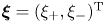 $\boldsymbol {\xi }=(\xi _+, \xi _-)^\textrm {T}$ and
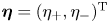 $\boldsymbol {\eta }=(\eta _+, \eta _-)^\textrm {T}$,
 \begin{align} \begin{pmatrix} {\boldsymbol{\xi}} \\ {\boldsymbol{\eta}} \end{pmatrix} =\begin{pmatrix} \boldsymbol{M}^{-1} & {\boldsymbol{O}} \\ {\boldsymbol{O}} & \boldsymbol{M}^{-1} {\boldsymbol{\varGamma}} \end{pmatrix} \begin{pmatrix} \boldsymbol{a} \\ \boldsymbol{b} \end{pmatrix},\quad \textrm{or} \quad \begin{pmatrix} \boldsymbol{a} \\ \boldsymbol{b} \end{pmatrix}=\begin{pmatrix} \boldsymbol{M} & {\boldsymbol{O}} \\ {\boldsymbol{O}} & {\boldsymbol{\varGamma}}^{-1}\boldsymbol{M} \end{pmatrix} \begin{pmatrix} {\boldsymbol{\xi}} \\ {\boldsymbol{\eta}} \end{pmatrix}, \end{align}
the linear system (B 1) can be written as
 \begin{equation} \frac{\textrm{d}}{\textrm{d} t} \begin{pmatrix} {\boldsymbol{\xi}} \\ {\boldsymbol{\eta}} \end{pmatrix} =\begin{pmatrix} {\boldsymbol{O}} & {\boldsymbol{I}} \\ {\boldsymbol{\varLambda}} & {\boldsymbol{O}} \end{pmatrix} \begin{pmatrix} {\boldsymbol{\xi}} \\ {\boldsymbol{\eta}} \end{pmatrix}, \end{equation}
where  $\boldsymbol {\xi }(-\boldsymbol {k},t)=\boldsymbol {\xi }^*(\boldsymbol {k},t)$ and
 $\boldsymbol {\eta }(-\boldsymbol {k},t)=\boldsymbol {\eta }^*(\boldsymbol {k},t)$ as
 $\gamma _{i,j}(-\boldsymbol {k})=\gamma _{i,j}(\boldsymbol {k})$.
Now, as  $\boldsymbol {\varLambda }$ and the identity matrix
 $\boldsymbol {I}$ in (B 9) are diagonal
 $2\times 2$ matrices, the surface and internal wave modes are decoupled as
 \begin{equation} \frac{\textrm{d} }{\textrm{d} t} \begin{pmatrix} \xi_\pm \\ \eta_\pm \end{pmatrix} =\begin{pmatrix} 0 & 1\\ -\omega_\pm^2 & 0 \end{pmatrix}\begin{pmatrix} \xi_\pm \\ \eta_\pm \end{pmatrix}, \end{equation}
where the positive and negative signs correspond to the surface and internal wave modes, respectively.
The nonlinear interaction between the surface and internal wave modes can be studied once a nonlinear system for  $\boldsymbol {\xi }$ and
 $\boldsymbol {\eta }$ is obtained. By substituting (B 8) into (A 1) and (A 2), or, directly from (3.30a,b), the evolution equations for
 $(\boldsymbol {\xi }, \boldsymbol {\eta })$ can be found as
 \begin{equation} \frac{\textrm{d}}{\textrm{d} t}\begin{pmatrix} {{\boldsymbol{\xi}}} \\ { {\boldsymbol{\eta}}} \end{pmatrix}=\begin{pmatrix} {\boldsymbol{O}} & {\boldsymbol{S}} \\ -{\boldsymbol{S}} & {\boldsymbol{O}} \end{pmatrix} \begin{pmatrix} {\delta H/ \delta {\boldsymbol{\xi}}^*} \\ {\delta H/ \delta {\boldsymbol{\eta} }^*} \end{pmatrix}, \end{equation}
where  ${\delta H/ \delta {\boldsymbol {\xi }}^*}= ({\delta H/ \delta \xi _+^*}, {\delta H/ \delta \xi _-^*} )^\textrm {T}$ and
 ${\delta H/ \delta {\boldsymbol {\eta }}^*}= ({\delta H/ \delta \eta _+^*}, {\delta H/ \delta \eta _-^*} )^\textrm {T}$. In (B 11),
 ${\boldsymbol {S}}$ is a
 $2\times 2$ matrix given by
 \begin{equation} {\boldsymbol{S}}=\boldsymbol{M}^{-1}{\boldsymbol{\varGamma}}\left (\boldsymbol{M}^{-1}\right )^\textrm{T}, \end{equation}
which yields a diagonal matrix so that  ${\boldsymbol {S}}=\textrm {diag} (s_+,s_- )$ with
 $s_\pm$ defined, with
 $\gamma _{12}=\gamma _{21}$, by
 \begin{align} \left.\begin{gathered} s_{+}=\frac{1}{n_+^2 } \frac{\left [ \left (\rho_u\gamma_{11}^2 -{\rm \Delta} \rho \gamma_{11}\gamma_{22}+2 {\rm \Delta} \rho \gamma_{12}^2 \right )\omega_+^2 -{\rm \Delta} \rho g \left (\rho_u\gamma_{11}-{\rm \Delta} \rho \gamma_{22}\right ) \left (\gamma_{11} \gamma_{22}-\gamma_{12}^2\right )\right ]} {g\left[ \rho_u\gamma_{11} \omega_+^2 -{\rm \Delta}\rho \gamma_{22} \omega_-^2 -2\rho_u {\rm \Delta}\rho g\left (\gamma_{11} \gamma_{22}-\gamma_{12}^2\right )\right ]^2},\\ s_{-}= \frac{1}{n_-^2 }\frac{\left [ \left ({\rm \Delta} \rho\gamma_{22}^2 - \rho_u \gamma_{11}\gamma_{22}+2 \rho_u \gamma_{12}^2 \right )\omega_-^2 +\rho_u g \left (\rho_u\gamma_{11}-{\rm \Delta} \rho \gamma_{22}\right ) \left (\gamma_{11} \gamma_{22}-\gamma_{12}^2\right )\right ]} {g\left[ \rho_u\gamma_{11} \omega_+^2 -{\rm \Delta}\rho \gamma_{22} \omega_-^2 -2\rho_u {\rm \Delta}\rho g\left (\gamma_{11} \gamma_{22}-\gamma_{12}^2\right )\right ]^2}. \end{gathered}\right\} \end{align}
To write (B 11) as Hamilton's equations, we further introduce  $\boldsymbol {q}$ and
 $\boldsymbol {p}$ defined as
 \begin{equation} \begin{pmatrix} {\boldsymbol{\xi}} \\ {\boldsymbol{\eta}} \end{pmatrix} =\begin{pmatrix} {\boldsymbol{S}}^{1/2} & {\boldsymbol{O}} \\ {\boldsymbol{O}} & {\boldsymbol{S}}^{1/2} \end{pmatrix}\begin{pmatrix} \boldsymbol{q} \\ \,\boldsymbol{p} \end{pmatrix}, \end{equation}
where  ${\boldsymbol {S}}^{1/2}=\textrm {diag} (s_+^{1/2},s_-^{1/2} )$,
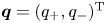 $\boldsymbol {q}=(q_+, q_-)^\textrm {T}$ and
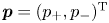 $\boldsymbol {p}=(p_+, p_-)^\textrm {T}$. Then, by substituting (B 14) into (B 11), the amplitude equations for
 $(\boldsymbol {q},\boldsymbol {p})$ can be obtained as Hamilton's equations:
 \begin{equation} \frac{\textrm{d}}{\textrm{d} t}\begin{pmatrix} {\boldsymbol{q}} \\ {\boldsymbol{p}} \end{pmatrix}=\begin{pmatrix} {\boldsymbol{O}} & \boldsymbol{I} \\ -\boldsymbol{I} & {\boldsymbol{O}} \end{pmatrix} \begin{pmatrix} {\delta H/ \delta \boldsymbol{q}^*} \\ {\delta H/ \delta \boldsymbol{p}^*} \end{pmatrix}. \end{equation}
Here the new conjugate variables  $q_\pm$ and
 $p_\pm$ are the generalized coordinates and momenta of the surface
 $(+)$ and internal
 $(-)$ wave modes, respectively. When (B 14) is combined with (B 8), the transformation (
 $\boldsymbol {a}$,
 $\boldsymbol {b}$) to
 $(\boldsymbol {q}, \boldsymbol {p})$ can be found as
 \begin{equation} \begin{pmatrix} \boldsymbol{a} \\ \boldsymbol{b} \end{pmatrix}=\begin{pmatrix} \boldsymbol{Q} & {\boldsymbol{O}} \\ {\boldsymbol{O}} & \boldsymbol{P} \end{pmatrix} \begin{pmatrix} \boldsymbol{q} \\ \boldsymbol{p} \end{pmatrix}, \end{equation}
where  $\boldsymbol {Q}$ and
 $\boldsymbol {P}$ are given by
 \begin{equation} \boldsymbol{Q}=\boldsymbol{M}{\boldsymbol{S}}^{1/2},\quad \boldsymbol{P}={\boldsymbol{\varGamma}}^{-1}\boldsymbol{M}{\boldsymbol{S}}^{1/2}. \end{equation}
Using this transformation, the amplitude equations for ( $q_\pm$,
 $p_\pm$) can be obtained, from (3.35a,b) with (3.33) and (3.34), as
 \begin{align} \frac{\partial q_+}{\partial t} &=p_+ +\iint[ (U^{(1)}_{-0,1,2}+ U^{(1)}_{1,-0,2} ) p_{1}^+ q_{2}^+ +U^{(2)}_{-0,1,2} \,p_{1}^- q_{2}^+ \nonumber\\ &\quad + (U^{(4)}_{-0,1,2}+ U^{(4)}_{1,-0,2} ) p_{1}^+ q_{2}^- + U^{(5)}_{-0,1,2} \,p_{1}^- q_{2}^- ] \delta_{0-1-2}\, \textrm{d}{\boldsymbol{k}}_{1,2} , \end{align}
 \begin{equation} \frac{\partial p_+}{\partial t}=-\omega_+^2 q_+ - \iint [ U^{(1)}_{1,2,-0}\kern0.05em p_{1}^+ p_{2}^+ + U^{(2)}_{1,2,-0}\kern0.05em p_{1}^+ p_{2}^- + U^{(3)}_{1,2,-0}\kern0.05em p_{1}^- p_{2}^- ] \delta_{0-1-2}\, \textrm{d}{\boldsymbol{k}}_{1,2} , \end{equation}
 \begin{align} \frac{\partial q_-}{\partial t}&=p_- +\iint [ U^{(2)}_{1,-0,2} \,p_{1}^+ q_{2}^+ +(U^{(3)}_{-0,1,2}+ U^{(3)}_{1,-0,2} ) p_{1}^- q_{2}^+ \nonumber\\ &\quad + U^{(5)}_{1,-0,2}\, p_{1}^+ q_{2}^- + (U^{(6)}_{-0,1,2}+ U^{(6)}_{1,-0,2} ) \,p_{1}^- q_{2}^- ] \delta_{0-1-2}\, \textrm{d}{\boldsymbol{k}}_{1,2} , \end{align}
 \begin{equation} \frac{\partial p_-}{\partial t}=-\omega_-^2 q_- - \iint [ U^{(4)}_{1,2,-0} p_{1}^+ p_{2}^+ + U^{(5)}_{1,2,-0} p_{1}^+ p_{2}^- + U^{(6)}_{1,2,-0} p_{1}^- p_{2}^- ] \delta_{0-1-2}\, \textrm{d}{\boldsymbol{k}}_{1,2} . \end{equation}
When discretized, this system can be considered a dynamical system for coupled oscillators.
On the other hand, the amplitude equations for the scalar complex amplitudes  $z_\pm$ introduced in (3.36) can be found, from (3.40), as
 \begin{align} \frac{\partial z_+}{\partial t} &= \textrm{i} \omega_+ z_+ + \textrm{i} \iint [ (V^{(1)}_{0,1,2} z^+_1 z^+_2+V^{(2)}_{0,1,2} z^+_1 z^-_2 + V^{(5)}_{0,1,2} z^-_1 z^-_2) \delta_{0-1-2} + \{(V^{(1)}_{2,0,1} \nonumber\\ &\quad + V^{(1)}_{2,1,0} ) {z^+_1}^* z^+_2 + V^{(2)}_{2,0,1} {z^-_1}^* z^+_2 + (V^{(3)}_{2,0,1}+ V^{(3)}_{2,1,0} ) {z^+_1}^* z^-_2 + V^{(4)}_{2,1,0} {z^-_1}^* z^-_2 \} \delta_{0+1-2}\nonumber\\ &\quad + \{(V^{(7)}_{0,1,2}+ V^{(7)}_{2,0,1} + V^{(7)}_{1,2,0} ) {z^+_1}^* {z^+_2}^*\nonumber\\ &\quad + (V^{(8)}_{0,1,2}+ V^{(8)}_{1,0,2} ) {z^+_1}^* {z^-_2}^* + V^{(9)}_{0,1,2} {z^-_1}^* {z^-_2}^* \} \delta_{0+1+2}] \textrm{d}\boldsymbol{k}_{1,2} , \end{align}
 \begin{align} \frac{\partial z_-}{\partial t} &= \textrm{i} \omega_- z_- +\textrm{i} \iint [ (V^{(3)}_{0,1,2} z^+_1 z^+_2 + V^{(4)}_{0,1,2} \, z^-_1 z^+_2 + V^{(6)}_{0,1,2} z^-_1 z^-_2) \delta_{0-1-2} +\{V^{(2)}_{2,1,0} {z^+_1}^* z^+_2\nonumber\\ &\quad + V^{(4)}_{2,0,1} {z^+_1}^* z^-_2 +(V^{(5)}_{2,0,1}+ V^{(5)}_{2,1,0} ) {z^-_1}^* z^+_2 +(V^{(6)}_{2,0,1}+ V^{(6)}_{2,1,0} ) {z^-_1}^* z^-_2 \} \delta_{0+1-2}\nonumber\\ &\quad + \{ V^{(8)}_{1,2,0} {z^+_1}^* {z^+_2}^* + (V^{(9)}_{2,0,1}+ V^{(9)}_{2,1,0} ) {z^-_1}^* {z^+_2}^*\nonumber\\ &\quad + (V^{(10)}_{0,1,2}+ V^{(8)}_{2,0,1} + V^{(10)}_{1,2,0} ) {z^-_1}^* {z^-_2}^* \} \delta_{0+1+2}] \textrm{d}\boldsymbol{k}_{1,2} . \end{align}
Appendix C. Interaction coefficients
The interaction coefficients  $U_{1,2,3}^{(n)}$ (
 $n=1,\ldots , 6$) for
 $H_3$ in (3.34) are given by
 \begin{align} U_{1,2,3}^{(1)}&=h_{1,2,3}^{(1)} P_1^{(1,1)}P_2^{(1,1)}Q_3^{(1,1)}+h_{1,2,3}^{(2)} P_1^{(1,1)}P_2^{(2,1)}Q_3^{(1,1)} +h_{1,2,3}^{(3)} P_1^{(2,1)}P_2^{(2,1)}Q_3^{(1,1)} \nonumber\\ &\quad +h_{1,2,3}^{(4)} P_1^{(1,1)}P_2^{(1,1)}Q_3^{(2,1)}+h_{1,2,3}^{(5)} P_1^{(1,1)}P_2^{(2,1)}Q_3^{(2,1)} +h_{1,2,3}^{(6)} P_1^{(2,1)}P_2^{(2,1)}Q_3^{(2,1)}, \end{align}
 \begin{align} U_{1,2,3}^{(2)}&=2h_{1,2,3}^{(1)} P_1^{(1,1)}P_2^{(1,2)}Q_3^{(1,1)} +h_{1,2,3}^{(2)} P_1^{(1,1)}P_2^{(2,2)}Q_3^{(1,1)}+ h_{2,1,3}^{(2)} P_1^{(2,1)}P_2^{(1,2)}Q_3^{(1,1)}\nonumber\\ &\quad +2h_{1,2,3}^{(3)} P_1^{(2,1)}P_2^{(2,2)}Q_3^{(1,1)} +2h_{1,2,3}^{(4)} P_1^{(1,1)}P_2^{(1,2)}Q_3^{(2,1)} \nonumber\\ &\quad +h_{1,2,3}^{(5)} P_1^{(1,1)}P_2^{(2,2)}Q_3^{(2,1)}+ h_{2,1,3}^{(5)} P_1^{(2,1)}P_2^{(1,2)}Q_3^{(2,1)} +2h_{1,2,3}^{(6)} P_1^{(2,1)}P_2^{(2,2)}Q_3^{(2,1)}, \end{align}
 \begin{align} U_{1,2,3}^{(3)}&=h_{1,2,3}^{(1)} P_1^{(1,2)}P_2^{(1,2)}Q_3^{(1,1)}+h_{1,2,3}^{(2)} P_1^{(1,2)}P_2^{(2,2)}Q_3^{(1,1)} +h_{1,2,3}^{(3)} P_1^{(2,2)}P_2^{(2,2)}Q_3^{(1,1)} \nonumber\\ &\quad +h_{1,2,3}^{(4)} P_1^{(1,2)}P_2^{(1,2)}Q_3^{(2,1)}+h_{1,2,3}^{(5)} P_1^{(1,2)}P_2^{(2,2)}Q_3^{(2,1)} +h_{1,2,3}^{(6)} P_1^{(2,2)}P_2^{(2,2)}Q_3^{(2,1)}, \end{align}
 \begin{align} U_{1,2,3}^{(4)}&=h_{1,2,3}^{(1)} P_1^{(1,1)}P_2^{(1,1)}Q_3^{(1,2)}+h_{1,2,3}^{(2)} P_1^{(1,1)}P_2^{(2,1)}Q_3^{(1,2)} +h_{1,2,3}^{(3)} P_1^{(2,1)}P_2^{(2,1)}Q_3^{(1,2)} \nonumber\\ &\quad +h_{1,2,3}^{(4)} P_1^{(1,1)}P_2^{(1,1)}Q_3^{(2,2)}+h_{1,2,3}^{(5)} P_1^{(1,1)}P_2^{(2,1)}Q_3^{(2,2)} +h_{1,2,3}^{(6)} P_1^{(2,1)}P_2^{(2,1)}Q_3^{(2,2)}, \end{align}
 \begin{align} U_{1,2,3}^{(5)}&=2h_{1,2,3}^{(1)} P_1^{(1,1)}P_2^{(1,2)}Q_3^{(1,2)} +h_{1,2,3}^{(2)} P_1^{(1,1)}P_2^{(2,2)}Q_3^{(1,2)}+ h_{2,1,3}^{(2)} P_1^{(2,1)}P_2^{(1,2)}Q_3^{(1,2)} \nonumber\\ &\quad +2h_{1,2,3}^{(3)} P_1^{(2,1)}P_2^{(2,2)}Q_3^{(1,2)} +2h_{1,2,3}^{(4)} P_1^{(1,1)}P_2^{(1,2)}Q_3^{(2,2)} \nonumber\\ &\quad +h_{1,2,3}^{(5)} P_1^{(1,1)}P_2^{(2,2)}Q_3^{(2,2)}+ h_{2,1,3}^{(5)} P_1^{(2,1)}P_2^{(1,2)}Q_3^{(2,2)} +2h_{1,2,3}^{(6)} P_1^{(2,1)}P_2^{(2,2)}Q_3^{(2,2)}, \end{align}
 \begin{align} U_{1,2,3}^{(6)}&=h_{1,2,3}^{(1)} P_1^{(1,2)} P_2^{(1,2)}Q_3^{(1,2)}+h_{1,2,3}^{(2)} P_1^{(1,2)}P_2^{(2,2)}Q_3^{(1,2)} +h_{1,2,3}^{(3)} P_1^{(2,2)}P_2^{(2,2)}Q_3^{(1,2)}\nonumber\\&\quad +h_{1,2,3}^{(4)} P_1^{(1,2)} P_2^{(1,2)}Q_3^{(2,2)}+h_{1,2,3}^{(5)} P_1^{(1,2)}P_2^{(2,2)}Q_3^{(2,2)} +h_{1,2,3}^{(6)} P_1^{(2,2)}P_2^{(2,2)}Q_3^{(2,2)}, \end{align}
where  $h_{1,2,3}^{(n)}$ are defined by (3.21)–(3.25), and (3.28) has been imposed. In addition,
 $Q^{(i,j)}$ and
 $P^{(i,j)}$ are defined as
 \begin{equation} \boldsymbol{Q}=\boldsymbol{M}{\boldsymbol{S}}^{1/2} =\begin{pmatrix} Q^{(1,1)} & Q^{(1,2)} \\ Q^{(2,1)} & Q^{(2,2)} \end{pmatrix}, \quad \boldsymbol{P}={\boldsymbol{\varGamma}}^{-1}\boldsymbol{M}{ \boldsymbol{S}}^{1/2} =\begin{pmatrix} P^{(1,1)} & P^{(1,2)} \\ P^{(2,1)} & P^{(2,2)} \end{pmatrix} , \end{equation}
with  $P^{(i,j)}_l=P^{(i,j)}(\boldsymbol {k}_l)$ and
 $Q^{(i,j)}_l=Q^{(i,j)}(\boldsymbol {k}_l)$.
After defining  ${\bar U}_{1,2,3}^{(n)}$ (
 $n=1,\ldots , 6$) as
 \begin{align} \left.\begin{gathered} {\bar U}^{(1)}_{1,2,3}=-\sqrt{\frac{\omega_1^+\omega_2^+}{8\omega_3^+}} U^{(1)}_{1,2,3},\quad {\bar U}^{(2)}_{1,2,3}=-\sqrt{\frac{\omega_1^+\omega_2^-}{8\omega_3^+}} U^{(2)}_{1,2,3},\quad {\bar U}^{(3)}_{1,2,3}=-\sqrt{\frac{\omega_1^-\omega_2^-}{8\omega_3^+}} U^{(3)}_{1,2,3}, \\ {\bar U}^{(4)}_{1,2,3}=-\sqrt{\frac{\omega_1^+\omega_2^+}{8\omega_3^-}} U^{(4)}_{1,2,3},\quad {\bar U}^{(5)}_{1,2,3}=-\sqrt{\frac{\omega_1^+\omega_2^-}{8\omega_3^-}} U^{(5)}_{1,2,3},\quad {\bar U}^{(6)}_{1,2,3}=-\sqrt{\frac{\omega_1^-\omega_2^-}{8\omega_3^-}} U^{(6)}_{1,2,3}, \end{gathered}\right\} \end{align}
the coefficients  $V_{1,2,3}^{(n)}$ (
 $n=1,\ldots , 10$) in (3.39) are given by
 \begin{align} \left.\begin{gathered} V_{1,2,3}^{(1)} = {{\bar{U}}}^{(1)}_{2,3,-1}-{{\bar{U}}}^{(1)}_{-1,2,3}-{{\bar{U}}}^{(1)}_{3,-1,2}, \quad V_{1,2,3}^{(2)}=- {{\bar{U}}}_{-1,3,2}^{(2)} + {{\bar{U}}}_{2,3,-1}^{(2)} -{{\bar{U}}}_{-1,2,3}^{(4)} -{{\bar{U}}}_{2,-1,3}^{(4)} ,\\ V_{1,2,3}^{(3)}=- {{\bar{U}}}_{3,-1,2}^{(2)} + {{\bar{U}}}_{2,3,-1}^{(4)} , \quad V_{1,2,3}^{(4)}= -{{\bar{U}}}_{-1,2,3}^{(3)} - {{\bar{U}}}_{2,-1,3}^{(3)} + {{\bar{U}}}_{3,2,-1}^{(5)} -{{\bar{U}}}_{3,-1,2}^{(5)}, \\ V_{1,2,3}^{(5)}= {{\bar{U}}}_{2,3,-1}^{(3)} - {{\bar{U}}}_{-1,2,3}^{(5)} , \quad V_{1,2,3}^{(6)}= {{\bar{U}}}_{2,3,-1}^{(6)} - {{\bar{U}}}_{-1,2,3}^{(6)} - {{\bar{U}}}_{3,-1,2}^{(6)} , \\ V_{1,2,3}^{(7)}={{\bar{U}}}_{1,2,3}^{(1)} , \quad V_{1,2,3}^{(8)}= {{\bar{U}}}_{1,3,2}^{(2)} + {{\bar{U}}}_{1,2,3}^{(4)} , \quad V_{1,2,3}^{(9)}= {{\bar{U}}}_{2,3,1}^{(3)} + {{\bar{U}}}_{1,2,3}^{(5)} ,\quad V_{1,2,3}^{(10)}={{\bar{U}}}_{1,2,3}^{(6)} , \end{gathered}\right\} \end{align}
where 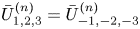 ${{\bar {U}}}_{1,2,3}^{(n)}={{\bar {U}}}_{-1,-2,-3}^{(n)}$
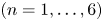 $(n=1,\ldots ,6)$ have been used. Note that
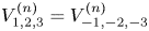 $V_{1,2,3}^{(n)}=V_{-1,-2,-3}^{(n)}$
 $(n=1,\ldots ,10)$.



