1. Introduction
Accurately measuring velocity fields is essential for advancing our understanding of complex fluid dynamics. Among various diagnostic techniques, particle image velocimetry (PIV) has emerged as one of the most sophisticated and widely adopted methods for capturing planar and volumetric velocity fields (Turhan, Wang & Gursul Reference Turhan, Wang and Gursul2022; Li et al. Reference Li, Feng, Wang and Liang2023; Zhu, Wang & Liu Reference Zhu, Wang and Liu2024). Leveraging high-resolution (HR) imaging and advanced cross-correlation algorithms, PIV enables the visualisation and quantification of intricate flow structures in applications ranging from fundamental turbulence research to aerodynamics, hydrodynamics and biomedical flows (Schröder & Willert Reference Schröder and Willert2008; Scarano Reference Scarano2012). Its ability to provide spatially resolved, instantaneous velocities has made it indispensable in experimental fluid mechanics. However, PIV is constrained by its spatio-temporal resolution limitations (Ozawa, Honda & Nonomura Reference Ozawa, Honda and Nonomura2024). In particular, the temporal resolution is governed by the frame rate of high-speed cameras and the repetition rate of illumination systems, rendering it incapable of achieving the temporal fidelity comparable to hot-wire anemometry for resolving rapid velocity fluctuations. Spatial resolution is similarly restricted by the camera’s pixel density and the optical magnification, which depend on the lens focal length and field of view. As a result, PIV struggles to capture small-scale turbulent structures and fine vortical features, especially in high Reynolds number flows where multi-scale interactions play a critical role.
To address the spatial and temporal resolution limitations of PIV, various traditional model-based reconstruction and super-resolution (SR) techniques have been proposed. In terms of spatial SR, spot-based correlation analysis combined with sub-interrogation particle tracking was developed to enhance resolution by up to a factor of 2.5 (Keane, Adrian & Zhang Reference Keane, Adrian and Zhang1995). Takehara et al. (Reference Takehara, Adrian, Etoh and Christensen2000) utilised Kalman filtering and advanced particle pairing techniques to achieve vector yields three to five times higher than those obtained with standard PIV, enabling more reliable velocity information obtained from highly turbulent flows. Direct numerical simulation (DNS)-based proper orthogonal decomposition (POD) modes combined with least-squares projection and Kriging interpolation were proposed to effectively recover near-wall structures and reduce noise, particularly in low-resolution (LR) experimental data (Gunes & Rist Reference Gunes and Rist2007). In addition, cross-projection using HR POD modes obtained from non-time-resolved PIV was employed to refine coarse time-resolved PIV data, enabling recovery of fine-scale structures while preserving accurate temporal dynamics (He & Liu Reference He and Liu2017). For enhancing temporal resolution, continuous space–time flow fields were reconstructed by POD-based time interpolation (Druault, Guibert & Alizon Reference Druault, Guibert and Alizon2005), which is capable of capturing the large-scale dynamics of pseudo-periodic flows, albeit with limitations in resolving small-scale structures (Bouhoubeiny & Druault Reference Bouhoubeiny and Druault2009). Durgesh & Naughton (Reference Durgesh and Naughton2010) proposed a multi-time-delay linear stochastic estimation approach combined with POD to reconstruct the low-order, time-resolved dynamics of coherent structures using surface pressure measurements. Correlation-based space–time reconstruction techniques leveraging POD coefficients were developed to recover phase-averaged flow fields from non-time-resolved ones (Legrand, Nogueira & Lecuona Reference Legrand, Nogueira and Lecuona2011). Furthermore, numerical solutions of the Navier–Stokes equations via the vortex-in-cell method enabled time supersampling of tomographic PIV data, allowing reconstruction of the detailed temporal dynamics even at subsampling rates far below the Nyquist frequency (Schneiders, Dwight & Scarano Reference Schneiders, Dwight and Scarano2014). Another physics-informed approach, proposed by Vamsi Krishna et al. (Reference Vamsi Krishna, Wang, Hemati and Luhar2020), employed rapid distortion theory and Taylor’s hypothesis to reconstruct time-resolved turbulent flow evolution between non-time-resolved PIV snapshots by fusing forward and backward temporal estimates.
Machine learning (ML), as a data-driven approach, excels at capturing complex flow dynamics without explicit physical modelling and has been widely applied in fluid dynamics (Brunton, Noack & Koumoutsakos Reference Brunton, Noack and Koumoutsakos2020). A data-driven method combining Voronoi tessellation and convolutional neural networks (CNNs) was developed to accurately recover complex flow fields from arbitrarily positioned, possibly moving sensors (Fukami et al. Reference Fukami, Maulik, Ramachandra, Fukagata and Taira2021b ). A hybrid data assimilation framework combining Bayesian ensemble filtering and echo state networks enhanced the accuracy of low-order thermoacoustic models, providing real-time estimates of system states and model bias under large uncertainties (Nóvoa & Magri Reference Nóvoa and Magri2022). A high-speed field-programmable gate array (FPGA)-based experimental deep reinforcement learning framework enabled real-time closed-loop flow control at 1–10 kHz, achieving rapid training within ten seconds and significantly enhancing shear layer mixing in supersonic flows (Zong et al. Reference Zong, Wu, Li, Su and Liang2025). A distributed control system integrating physics-informed ML control was experimentally demonstrated to adaptively suppress flow separation, achieving full flow reattachment and a 125 % base pressure increase on a backward-facing ramp at a Reynolds number of 32 000 (Jiang et al. Reference Jiang, Maceda, Guy, Wang, Gao and Noack2025). In addition, ML has been widely applied to SR reconstruction of flow fields, primarily using CNNs and artificial neural networks (ANNs). The CNN-based methods, including hybrid downsampled skip-connection/multi-scale models (Fukami, Fukagata & Taira Reference Fukami, Fukagata and Taira2019, Reference Fukami, Fukagata and Taira2021a ), U-Nets (Pant & Farimani Reference Pant and Farimani2020; Hu et al. Reference Hu, Yin, Hamrani, Leon and McDaniel2024) and variants incorporating temporal inputs, skip connections or physical constraints (Liu et al. Reference Liu, Tang, Huang and Lu2020; Cheng & Zhang Reference Cheng and Zhang2021; Yasuda et al. Reference Yasuda, Onishi, Hirokawa, Kolomenskiy and Sugiyama2022), have shown strong capability in reconstructing HR laminar and turbulent flows from coarse data. The ANN-based approaches, such as sinusoidal representation networks (Saitta et al. Reference Saitta, Carioni, Mukherjee, Schönlieb and Redaelli2024), multi-layer perceptron (MLP) networks for sparse-sensor reconstruction (Nair & Goza Reference Nair and Goza2020; Manohar, Morton & Ziadé Reference Manohar, Morton and Ziadé2022) and hybrid MLP–CNN models (Morimoto et al. Reference Morimoto, Fukami, Maulik, Vinuesa and Fukagata2022; Zhong et al. Reference Zhong, Fukami, An and Taira2022), also enhance reconstruction accuracy while reducing computational cost. Although CNN-based and ANN-based models have achieved SR reconstruction in various domains, their ability to recover fine-scale and HR flow features remains limited, often resulting in smoothed small-scale structures, as observed in the subsonic jet (Ozawa et al. Reference Ozawa, Honda and Nonomura2024) and homogeneous isotropic turbulence (Nista et al. Reference Nista, Pitsch, Schumann, Bode, Grenga, MacArt and Attili2024).
This limitation primarily stems from their reliance on direct input–output regression. In contrast, generative models aim to learn the underlying data distribution, offering improved generalisation and finer structural recovery. The SR generative adversarial networks (SRGANs), initially proposed by Ledig et al. (Reference Ledig2017), have demonstrated superior performance in capturing detailed HR features compared with CNN-based models. The GAN-based approaches successfully achieved SR reconstruction of small-scale turbulent flow features and exhibited strong out-of-sample robustness (Nista et al. Reference Nista, Pitsch, Schumann, Bode, Grenga, MacArt and Attili2024). Furthermore, Li et al. (Reference Li, Han, Zhang, Fu, Li, Qin, Dong, Sun, Deng and Yang2024) utilised a sparse-sensor-assisted score-based generative model to enable zero-shot reconstruction and prediction of the full-field spatio-temporal dynamics from extremely sparse and noisy measurements. Building on the original SRGAN framework, Wang et al. (Reference Wang, Yu, Wu, Gu, Liu, Dong, Qiao and Change Loy2018) refined the model architecture and loss functions to propose the enhanced SRGAN (ESRGAN), which further improved SR reconstruction capability. The ESRGAN-based architectures have since been applied to HR flow field reconstructions. Yousif et al. (Reference Yousif, Yu and Lim2021, Reference Yousif, Yu and Lim2022) employed ESRGAN to reconstruct HR laminar and turbulent flow fields from extremely coarse data at a wide range of Reynolds numbers, while Yu et al. (Reference Yu, Yousif, Zhang, Hoyas, Vinuesa and Lim2022) extended this framework to reconstruct three-dimensional velocity fields in channel flows, demonstrating strong agreement with DNS references even when trained on limited data. However, these GAN-based SR studies have primarily relied on numerically generated data as input, which are theoretically noise free and do not account for the measurement noise typically present in experimental results, where such noise should be carefully considered as it may increase the difficulty of accurate SR reconstruction (Fukami, Fukagata & Taira Reference Fukami, Fukagata and Taira2024). Deng et al. (Reference Deng, He, Liu and Kim2019) leveraged ESRGAN to recover HR turbulent velocity fields from LR PIV data. Nevertheless, research focusing on GAN-based SR models using experimental data remains scarce and existing studies predominantly address spatial SR of velocity fields, with limited attention given to temporal SR. Furthermore, the generalisation capability and efficiency gains of GAN-based SR models when applied to experimental data have not yet been fully explored.
Therefore, there are three objectives of this work. First, based on the ESRGAN model proposed by Wang et al. (Reference Wang, Yu, Wu, Gu, Liu, Dong, Qiao and Change Loy2018), we aim to achieve spatial SR reconstruction of PIV-measured vortex flows, capturing various stages including its formation, growth, transition and breakdown processes. Second, we introduce a dataset construction strategy along the temporal dimension to enable ESRGAN to perform temporal SR reconstruction on PIV data. Third, we evaluate the generalisation capability of this GAN-based spatio-temporal SR model under different flow conditions, as well as the efficiency gains it brings to PIV data analysis. Following the introduction, § 2.1 details the structure of the ESRGAN model used in this study, including the configurations of the generator and discriminator, the formulation of the loss functions and the specific training parameters. Sections 2.2 and 2.3 describe the PIV measurement methods for plasma-induced vortex flows, the post-processing procedures and the division of datasets for model training. In §§ 3.2, 3.3 and 3.1, the spatio-temporal SR reconstruction performance of ESRGAN is assessed under different SR factors for time-averaged, instantaneous and phase-averaged velocity fields, where flow statistics such as Reynolds stress fields, POD modes and plasma thrust are thoroughly compared. In § 3.4, the model’s generalisation capability is examined by applying it to flows with both a similar and an entirely different vortex dynamics, and transfer learning is introduced to further improve reconstruction accuracy. In § 3.5, we analyse the efficiency benefits of applying the GAN-based spatio-temporal SR model to PIV data analysis, as well as the limitations inherent to its SR capability. Finally, the conclusions are summarised in § 4.
2. Methodology
2.1. Generative adversarial network models
The purpose of this study is to reconstruct high spatio-temporal resolution flow fields (
 $x \times y \times t$
) from corresponding LR fields (
 $\alpha x \times \alpha y \times \beta t$
), where
 $x$
is the streamwise direction,
 $y$
is the vertical direction and
 $t$
denotes temporal direction, as illustrated in figure 1(a). Here,
 $\alpha$
and
 $\beta$
represent the downsampling ratios in space and time, respectively. In this study,
 $\alpha$
is set to
 $(1/4)$
,
 $(1/8)$
and
 $(1/16)$
, while
 $\beta$
is fixed at
 $(1/4)$
, leading to
 $\times$
4,
 $\times$
8 and
 $\times$
16 spatial SR and
 $\times$
4 temporal SR. The process of generating the LR data is described in § 2.3. To achieve high-fidelity reconstruction of multi-scale vortical structures, the ESRGAN framework is adopted due to its superior capability in capturing high-frequency flow features (Ledig et al. Reference Ledig2017; Wang et al. Reference Wang, Yu, Wu, Gu, Liu, Dong, Qiao and Change Loy2018). Unlike the conventional ESRGAN, which performs only spatial SR on single frames, the present work develops a sequential framework in which two independent ESRGAN models are trained separately and then coupled to achieve spatio-temporal SR of flow fields while accounting for measurement noise. In addition, transfer learning is employed to enhance the generalisation capability of the GAN-based spatio-temporal SR model, enabling accurate reconstruction across multiple flow conditions with different vortex dynamics. Similar to conventional GAN-based approaches, the ESRGAN framework consists of a generator G and a discriminator D, whose architectures are depicted in figures 1(b) and 1(c), respectively, with c denoting the number of output channels, k the kernel size and s the stride.
(a) Sketch of reconstruction from LR input (
 $\alpha x \times \alpha y \times \beta t$
) to HR flow fields (
 $x \times y \times t$
), (b) architecture of the generator G and (c) architecture of the discriminator D, with c denoting the number of output channels, k the kernel size and s the stride.

The generator network G, shown in figure 1(b), begins with an initial convolutional layer (c64k3s1), which maps the input to a higher-dimensional feature space. This is followed by 23 residual-in-residual dense blocks (RRDB), each composed of five convolutional layers (e.g. c32k3s1, c64k3s1), four leaky rectified linear unit (leakyReLU) activations and intermediate skip connections to facilitate efficient feature reuse and mitigate vanishing gradient problems. Within each RRDB, residual scaling of 0.2 is applied to stabilise training. Notably, no batch normalisation (BN) layers are used in G to avoid over-smoothing and preserve fine-scale flow details. After the RRDB stack, upsampling is conducted via up-convolution layers, which adopt a nearest-neighbour interpolation strategy to gradually reconstruct the spatial and temporal resolutions. Finally, the output is refined using additional convolutional layers to match the input channels.
The discriminator network D, as shown in figure 1(c), is designed to distinguish between reconstructed and reference HR flow fields. It comprises a series of convolutional layers with progressively increasing channels (from 64 to 1024) and decreasing feature map resolutions, interleaved with leakyReLU activations (negative slope = 0.2) and BN layers to improve learning stability. An adaptive average pooling layer is incorporated before the final fully connected layers to aggregate spatial information and enable consistent classification regardless of input resolution.
To achieve spatio-temporal SR reconstruction, two separate ESRGAN models are employed, denoted as SESRGAN (for spatial SR) and TESRGAN (for temporal SR) for clarity. These two models share an identical architecture (see figure 1), except for the upsampling design in the generator G, which is adapted according to the input dimensionality. Specifically, SESRGAN aims to reconstruct the spatial resolution from
 $\alpha x \times \alpha y$
to the target resolution
 $x \times y$
, while TESRGAN is designed to recover temporal resolution from
 $\beta t$
to
 $t$
, taking
 $y \times \beta t$
as input (with
 $y$
representing the already refined spatial dimension). In SESRGAN, the upsampling block of G focuses on enlarging both spatial dimensions simultaneously to achieve the target HR spatial field. In contrast, TESRGAN only performs upsampling along the temporal dimension without altering the spatial resolution.
It is important to note that, due to the adoption of two sequential ESRGAN models, the ordering of spatial and temporal SR becomes a critical consideration. The LR data are generated via average pooling from HR PIV data (see § 2.3). Consequently, performing temporal SR before spatial SR is infeasible, as it would prevent accurate alignment between the LR input and the target HR ground truth necessary for supervised learning. Therefore, for PIV datasets, the spatio-temporal SR framework based on ESRGAN can only be implemented in a spatial-to-temporal order. Moreover, Fukami et al. (Reference Fukami, Fukagata and Taira2021a ) also indicated that adopting the spatial-to-temporal order yields superior reconstruction accuracy and perceptual quality compared with the reverse order.
To improve the realism and stability of the reconstructed flow fields, this study adopts the relativistic average GAN (RaGAN) loss instead of the standard GAN loss (Jolicoeur-Martineau Reference Jolicoeur-Martineau2018). In conventional GANs, the discriminator independently estimates the probability of each sample being real, which often leads to overconfident predictions and vanishing gradients for the generator. In contrast, RaGAN considers the relative realism between real and generated samples, providing more informative gradient feedback and thus improving convergence. Accordingly, the adversarial loss for the generator is defined as
 \begin{equation} \mathcal{L}_{\textit{ad}v} = -\mathbb{E}_{z}\left [\log \bigl (1 - \sigma (D(z) - \mathbb{E}_{\hat {z}}[D(\hat {z})])\bigr )\right ] - \mathbb{E}_{\hat {z}}\left [\log \sigma (D(\hat {z}) - \mathbb{E}_{z}[D(z)])\right]\!, \end{equation}
where
 $z$
denotes the ground-truth (PIV reference) sample,
 $\hat {z}$
the generated sample,
 $D(\boldsymbol{\cdot })$
the discriminator output,
 $\sigma (\boldsymbol{\cdot })$
the sigmoid function and
 $\mathbb{E}[\boldsymbol{\cdot }]$
the expectation operator over the data distribution. The discriminator loss is given by
 \begin{equation} \mathcal{L}_{D} = -\mathbb{E}_{z}\left [\log \sigma (D(z) - \mathbb{E}_{\hat {z}}[D(\hat {z})])\right ] - \mathbb{E}_{\hat {z}}\left [\log \bigl (1 - \sigma (D(\hat {z}) - \mathbb{E}_{z}[D(z)])\bigr )\right]\!. \end{equation}
In addition to the adversarial loss, the generator loss incorporates a content loss and a perceptual loss to enforce pixel-level accuracy and perceptual quality. The content loss is defined as
 \begin{equation} \mathcal{L}_{\textit{content}} = \lVert \hat {z} - z \rVert _2^2. \end{equation}
The perceptual loss is expressed as
 \begin{equation} \mathcal{L}_{\textit{perc}} = \lVert \varPhi (\hat {z}) - \varPhi (z) \rVert _2^2, \end{equation}
where
 $\varPhi (\boldsymbol{\cdot })$
denotes the feature extraction function from a pre-trained visual geometry group (VGG)-16 network, which is selected because it has been widely demonstrated to effectively capture high-frequency information in GAN-based SR frameworks (Ledig et al. Reference Ledig2017; Wang et al. Reference Wang, Yu, Wu, Gu, Liu, Dong, Qiao and Change Loy2018), thereby providing rich hierarchical features that enhance the reconstruction of fine-scale structures. In this study, features are extracted before the activation layer up to the 28th convolutional layer. Finally, the total generator loss is formulated as
 \begin{equation} \mathcal{L}_{G} = \gamma _1 \, \mathcal{L}_{\textit{content}} + \gamma _2 \, \mathcal{L}_{\textit{ad}v} + \gamma _3 \, \mathcal{L}_{\textit{perc}}, \end{equation}
where the weights are empirically set to
 $\gamma _1 = 1000$
,
 $\gamma _2 = 1$
and
 $\gamma _3 = 2$
, as suggested by Yousif, Yu & Lim (Reference Yousif, Yu and Lim2022).
The training process is implemented using the Adam optimiser with a learning rate of
 $1\times 10^{-4}$
for both the generator and the discriminator. The batch size is set to 64 for SESRGAN and reduced to 32 for TESRGAN to accelerate training, considering the increased memory consumption along the
 $y$
-axis resolution. The total number of epochs is set to 800 for SESRGAN and 300 for TESRGAN to ensure convergence. All models are trained using the PyTorch framework on an NVIDIA RTX 4090 GPU to handle HR flow field data and large-scale model parameters efficiently.
2.2. Experimental set-up
To validate the capability of the ESRGAN framework in achieving spatio-temporal SR for multi-scale vortex structures, training data are acquired from plasma-induced vortex pairs generated by dielectric barrier discharge plasma actuators in quiescent air, as shown in figure 2(a). Two plasma actuators are symmetrically mounted on both sides of a 3-mm-thick aluminium composite flat plate, with the trailing edge of the encapsulated electrode aligned with the plate tip. Each actuator comprises an exposed electrode, dielectric layers and an encapsulated electrode. The exposed and encapsulated electrodes are fabricated from 0.05 mm-thick, 10 mm-wide copper foil tapes, separated by two 0.15 mm-thick Cirlex sheets. The actuators are powered by a Minipuls 6 AC supply delivering a sinusoidal voltage with a peak-to-peak amplitude
 $E_{pp}$
of 18 kV at 7 kHz. To periodically generate vortex pairs, this voltage is externally modulated by a 5 V square waveform with a frequency of
 $f_m$
= 20 Hz and a duty cycle of 50 % produced by a FPGA on a National Instruments CompactRIO controller, as illustrated in figure 2(b).
(a) Schematic of the experimental set-up (not to scale). All dimensions are in millimetres. (b) Illustration of the sinusoidal AC excitation voltage modulated by a square wave.

The actuators are centrally mounted in a sealed transparent acrylic box (600 mm
 $\times$
300 mm
 $\times$
300 mm) on a 150 mm-long 3D-printed strut. A Litron LDY 302-PIV Nd dual-cavity laser is positioned above the box using a laser guide arm to generate a 0.5 mm-thick laser sheet, with a pulse interval of 100
 $\unicode{x03BC}$
s. A CMOS high-speed camera equipped with a 110 mm Canon lens is placed laterally to capture time-resolved, two-dimensional velocity fields at a resolution of 1280
 $\times$
800 pixels and a sampling rate of
 $f_s$
= 960 Hz. To minimise wall effects on vortex evolution, the actuators are positioned 300 mm from the downstream wall and 150 mm from the side walls. The PIV measurement region, indicated in figure 2(a), covers 95 mm
 $\times$
155 mm and captures vortex formation, growth, transition and breakdown processes (Dong et al. Reference Dong, Zhang, Ren, Yang, Xiao, Yao and Mao2025). The coordinate origin is defined at the plate tip, with
 $U$
and
 $V$
representing the streamwise and vertical velocity components, respectively. Before each measurement, the box is seeded with di-ethyl-hexyl-sebacate particles of approximately 1
 $\unicode{x03BC}$
m in diameter and left to settle for 10 minutes to ensure quiescence. The plasma actuators, laser pulses and camera are synchronised by a timing box with a delay of less than 5
 $\unicode{x03BC}$
s to ensure accurate capture of the starting vortices. Each PIV recording lasts 4 s, comprising 0.5 s of pre-discharge recording to confirm quiescence, 3 s of plasma-induced flow measurement and 0.5 s of post-discharge relaxation.
2.3. Data post-processing
The raw particle images are processed into corresponding velocity fields using Dantec DynamicStudio 2015a software. Adaptive correlation analysis is employed, which iteratively refines the interrogation windows by adjusting their size and shape based on local particle density and displacement gradients, thereby improving measurement accuracy near strong shear or vortical regions. The choice of interrogation area (IA) size is critical, as it directly determines the spatial resolution and the ability to resolve fine-scale flow structures. The velocity vector obtained within each IA represents the averaged motion of all particles in that region. For generating the PIV reference data used to train the ESRGAN model, minimum IAs are set to 16
 $\times$
16 pixels with 50 % overlap, yielding approximately 16 000 velocity vectors per frame. Outlier detection is applied by replacing erroneous vectors with the median of a 3
 $\times$
3 neighbourhood to ensure data reliability. The measurement error is evaluated by considering the shift distance of seeding particles and the inter-frame time interval, following the method proposed by Kline (Reference Kline1963), and is estimated to be below 5 % (Dong et al. Reference Dong, Choi and Wang2022b
).
To ensure the quality of the PIV data and fully capture the vortex evolution from formation to breakdown, the region from
 $x = 0$
to 120 mm and
 $y = -30$
to 30 mm is selected as the SR domain, as illustrated in figure 2(a). Consequently, a total of 2880 time-resolved two-dimensional PIV snapshots are collected, with spatio-temporal dimensions of
 $N_x \times N_y \times N_t = 128 \times 64 \times 2880$
, where
 $N_x$
and
 $N_y$
denote the spatial resolution in the
 $x$
and
 $y$
directions, respectively, and
 $N_t$
represents the number of PIV frames. These data serve as HR PIV reference fields for model training.
The LR PIV data are ideally obtained by enlarging the IA size, thereby averaging the displacements of all particles contained within the IA to calculate the velocity vector. Since the raw particle images of the present vortex-induced flow are not available, the LR fields are constructed by average pooling of the HR velocity vectors, as illustrated in figure 3(a). This method is validated using PIV data of a NACA0012 airfoil, where the LR fields obtained by average pooling match those obtained by direct analysis with larger IA, confirming that this approach preserves the key characteristics of LR PIV data, including noise features. Specifically, for each time step, LR fields with
 $\alpha = (1/4), (1/8)$
and
 $(1/16)$
are produced by averaging over
 $4 \times 4$
,
 $8 \times 8$
and
 $16 \times 16$
neighbouring velocity vectors, respectively. Paired HR and LR data are then used to train the SESRGAN model. The HR reference sequences for temporal SR are extracted directly from the original PIV measurements, defined as segments of 128 consecutive time steps. Corresponding low-temporal-resolution data are obtained from SESRGAN-reconstructed HR flow fields by selecting every fourth time step within each segment, resulting in
 $\beta = (1/4)$
, as shown in figure 3(b). The spatial resolution in the
 $y$
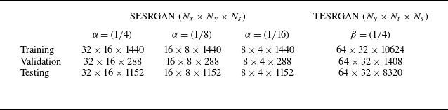
direction remains unchanged to avoid introducing uncorrelated discrepancies between LR inputs and HR references. Each TESRGAN input consists of 128 consecutive time steps, while each plasma pulse only contains 48 time-resolved PIV snapshots, giving limited number of available training samples. To expand the dataset, overlapping sequences are generated by shifting the starting point of each sequence by 16 time steps (approximately one third of a pulse period). Consequently, instead of extracting one non-overlapping sequence every 128 steps, this overlap strategy yields nearly eight times more training samples. The dataset is divided into three subsets: 30 discharge pulses for training, 6 pulses for validation and 24 pulses for testing. Detailed sample inputs used for the SESRGAN and TESRGAN models are summarised in table 1, where
 $N_s$
denotes the number of samples.
Illustration of the spatial downsampling for SESRGAN training (a) and the temporal downsampling for TESRGAN training (b).

Summary of dataset configurations for SESRGAN and TESRGAN training.

To enable the use of the pre-trained VGG-16 model for perceptual loss calculation (see § 2.1), which requires a three-channel input, the training data are constructed using the streamwise velocity
 $U$
, the vertical velocity
 $V$
and the root mean square (r.m.s.) of
 $U$
and
 $V$
. The network consequently outputs HR reconstructions for each channel. Note that the choice of using the r.m.s. of
 $U$
and
 $V$
as the third channel is intended to highlight the potential of the proposed model for spatio-temporal SR reconstruction of three-dimensional velocity fields, where the r.m.s. channel can be directly replaced by the spanwise velocity component
 $W$
when applied to three-dimensional cases. Normalisation is applied to improve stability during training and to ensure that different velocity components contribute comparably to the loss functions. Considering that the plasma-induced flow here is dominated by the streamwise velocity,
 $U$
and
 $V$
are normalised to [0, 1] using min–max scaling, as suggested by Deng et al. (Reference Deng, He, Liu and Kim2019), expressed as
 \begin{equation} U^* = \frac {U - U_{\textit{min }}}{U_{\textit{max }} - U_{\textit{min }}}, \quad V^* = \frac {V - V_{\textit{min }}}{V_{\textit{max }} - V_{\textit{min }}}, \end{equation}
where
 $U_{\textit{min }}$
and
 $U_{\textit{max }}$
represent the minimum and maximum values of
 $U$
within the entire dataset, respectively, and similarly for
 $V$
.
3. Results
To evaluate the performance of the proposed model, detailed qualitative and quantitative comparisons are conducted between the reconstructed HR flow fields (obtained from different LR inputs) and the PIV reference data in this section. For clarity, the case denoted as
 $\times$
4 spatio-temporal SR corresponds to input data with
 $(\alpha , \beta ) = ((1/4), (1/4))$
, while the
 $\times$
8 and
 $\times$
16 cases correspond to
 $(\alpha , \beta ) = ((1/8), (1/4))$
and
 $(\alpha , \beta ) = ((1/16), (1/4))$
, respectively. For comparison, the
 $x$
and
 $y$
coordinates are non-dimensionalised using the flat plate thickness
 $k$
, defined as
 $x^* = x / k$
and
 $y^* = y / k$
, while the time is non-dimensionalised using the modulation frequency
 $f_m$
, expressed as
 $\tau ^* = t f_m$
.
3.1. Spatio-temporal reconstruction of time-averaged velocity fields
The comparison of the time-averaged flow fields between the reconstructed results and the PIV reference is presented in figure 4. It can be seen that the
 $\times$
4,
 $\times$
8 and
 $\times$
16 SR cases are able to accurately reconstruct the distribution and magnitude of both
 $U^*$
and
 $V^*$
components, successfully capturing the jet spreading and velocity decay along the streamwise direction. This is because time averaging substantially suppresses the small-scale coherent vortical structures, reducing instantaneous fluctuation effects and enhancing the large-scale flow features, which allows even the
 $\times$
16 case to recover the main jet characteristics effectively. However, as the SR factor increases, the reconstruction accuracy gradually decreases, particularly in regions close to the plasma actuator (
 $x^* \lt 5$
in figure 4
b). The corresponding Reynolds stress fields
 $-\overline {uv}$
are shown in figure 4(c). The
 $\times$
4 and
 $\times$
8 cases successfully reconstruct the primary stress distribution, including the strong dipole structures near the plasma actuator and the extended high-shear regions farther downstream. These accurately captured stress fields reflect the models’ ability to reconstruct essential turbulent momentum transport, which is critical for jet spreading and cross-stream mixing processes. In contrast, although the
 $\times$
16 case captures the general shape of the stress field, it exhibits more pronounced discrepancies in both spatial continuity and stress intensity. This can be attributed to its limited capability to recover fluctuating velocity components.
Comparison of time-averaged flow fields between the reconstructed results and the PIV reference: (a) streamwise velocity
 $U^*$
, (b) vertical velocity
 $V^*$
and (c) Reynolds stress
 $-\overline {uv}$
. The white lines in the upper-left panel illustrate the jet width
 $w_{\!j}$
.

The comparison of the time-averaged maximum streamwise velocity
 $U_m$
along the jet direction between the reconstructed fields and the PIV reference is presented in figure 5(a). All SR cases closely follow the PIV reference, accurately capturing the rapid acceleration in the near field (
 $x^* \lt 10$
), the gradual decay downstream (
 $x^* \gt 15$
) and finally approaching a plateau. This demonstrates that the model can successfully recover the core jet momentum distribution even at high SR factors. Given that plasma jets are primarily used for active flow control (Corke, Enloe & Wilkinson Reference Corke, Enloe and Wilkinson2010; Wang et al. Reference Wang, Choi, Feng, Jukes and Whalley2013), the plasma-induced forcing plays a critical role in determining control effectiveness. Therefore, the plasma thrust per unit width
 $M_x$
(Jukes & Choi Reference Jukes and Choi2009), defined as
 \begin{equation} M_x = \int \rho U^{*2} \mathrm{d}y^*, \end{equation}
where
 $\rho$
is the air density, is analysed along the streamwise direction, as shown in figure 5(b). It can be seen that the proposed model accurately reconstructs the jet forcing at all SR factors, demonstrating its potential for evaluating plasma jet control performance. Furthermore, the jet entrainment coefficient
 $\mu$
(Hussein, Capp & George Reference Hussein, Capp and George1994), defined as
 \begin{equation} \mu = \dfrac {\int _{-\infty }^{\infty } \dfrac {U^*}{U_m} \dfrac {y^*}{x^*} \mathrm{d} \dfrac {y^*}{x^*} }{ \sqrt {\int _{-\infty }^{\infty } \dfrac {U^{*2}}{U_m^2} \dfrac {y^*}{x^*} \mathrm{d} \dfrac {y^*}{x^*}} }, \end{equation}
is computed and presented in figure 5(c). Similarly, all SR cases successfully capture the evolution of
 $\mu$
, confirming the superior capability of the proposed spatio-temporal SR model in accurately reconstructing time-averaged jet flow fields.
Quantitative comparison of time-averaged jets reconstructed by different SR cases and the PIV reference: (a) streamwise variation of the maximum velocity
 $U_m$
, (b) plasma thrust per unit width
 $M_x$
and (c) jet entrainment coefficient
 $\mu$
.

Comparison of the vertical spreading of the plasma jet: (a) streamwise evolution of the jet width
 $w_{\!j}$
and (b) normalised streamwise velocity profiles at
 $x^* = 5$
.

The vertical spreading behaviour of the plasma jet is further evaluated and compared in figure 6. The jet width
 $w_{\!j}$
is defined at the location where
 $U^* = 0.5 U_m(x^*)$
, as illustrated in figure 4. Due to the symmetric arrangement of the plasma actuators on both sides of the flat plate, a step-like separation region forms near the plasma actuators (figure 4
a). Therefore, the jet width is considered only for
 $x^* \gt 2$
to avoid initial separation effects. It is evident that all SR cases accurately capture both the initial jet contraction induced by plate effects and the downstream jet spreading driven by enhanced vertical momentum transfer due to vortex breakdown. The reconstructed jet widths are in excellent agreement with the PIV reference data in the entire range. Moreover, for symmetric jets, the vertical velocity profiles are expected to exhibit self-similar behaviour (Hussein et al. Reference Hussein, Capp and George1994). In this analysis, the velocity is normalised by the local maximum velocity
 $U_m$
and the
 $y$
-coordinate is non-dimensionalised using both the centreline position
 $y_m$
and the jet width
 $w_{\!j}$
. Theoretically, the peak streamwise velocity should appear at the centreline (
 $y^* = 0$
). However, slight random lateral displacements of the peak are observed in plasma jets, a phenomenon also reported in studies of plasma synthetic jets (Zong & Kotsonis Reference Zong and Kotsonis2018). Figure 6(b) shows the normalised streamwise velocity profiles at
 $x^* = 5$
. Profiles at other streamwise positions show similar trends and are thus not presented here for clarity. The
 $\times$
4 and
 $\times$
8 SR cases produce velocity profiles nearly identical to the PIV reference, demonstrating a Gaussian-like distribution. In contrast, the
 $\times$
16 case maintains good agreement only within
 $-1 \lt (y^*-y_m)/w_{\!j} \lt 1$
, while larger reconstruction errors are observed outside this core region, especially near the edges of the PIV measurement domain, where the velocities are much lower compared with the jet core.
3.2. Spatio-temporal reconstruction of instantaneous velocity fields
The model-reconstructed instantaneous streamwise and vertical velocities over 10 pulses are compared with the reference PIV results in figure 7, at different vertical locations with
 $y^* = 0$
and 4. At
 $x^* = 5$
, where the flow is dominated by the shear layer flow at
 $y^* = 0$
and periodic coherent vortices at
 $y^* = 4$
, all reconstructed curves closely match the PIV reference data, accurately capturing the primary periodic oscillations and amplitude variations. Only minor deviations are observed in the
 $\times$
16 case for the
 $V^*$
-component at
 $y^* = 0$
and the
 $U^*$
-component at
 $y^* = 4$
, primarily manifested as an underestimation of local peaks, reflecting the difficulty in reconstructing fine-scale structures from highly downsampled inputs. As
 $x^*$
increases to 20 and 35, corresponding to the transition and breakdown regions, the flow exhibits more irregular temporal fluctuations due to vortex deformation and increased turbulence. Despite the presence of small-scale fluctuations, the overall temporal trends of both velocity components remain well reconstructed. Noticeable discrepancies still appear in the
 $\times$
16 case, which can be attributed to the limited information in the highly downsampled inputs, making it challenging to accurately recover small-scale unsteady features. Overall, the two-component instantaneous velocities are successfully reconstructed within both large-scale and small-scale vortex regions. However, the reconstruction accuracy naturally decreases as the downsampling factor increases.
Comparison of reconstructed and PIV-measured HR instantaneous velocities over 10 pulses at different vertical locations for (a)
 $y^* = 0$
and (b)
 $y^* = 4$
. The left and right columns correspond to the streamwise velocity
 $U^*$
and the vertical velocity
 $V^*$
, respectively. The sampling location in the flow field is indicated at the top.

Figure 8 compares the instantaneous streamwise and vertical velocity peaks obtained from the model SR reconstructions and the PIV reference data, where
 $\hat {U}$
and
 $\hat {V}$
denote the reconstructed velocities. The probability density of different velocity magnitudes is indicated by the colour scale. For the
 $\times$
4 case (figure 8
a), most peak velocities and the high-density region align closely along the diagonal line, indicating excellent agreement between the reconstructed and PIV reference velocities for both components. In the
 $\times$
8 case (figure 8
b), the peak velocities remain concentrated near the diagonal, though a slight upward deviation is observed at higher velocity magnitudes, suggesting a minor underestimation of peak values by the model. For the
 $\times$
16 case (figure 8
c), the velocities exhibit a more noticeable spread from the diagonal, although the overall trend is still well captured. This increased dispersion indicates reduced accuracy in reconstructing fine-scale velocity peaks, consistent with the temporal velocity variations observed in figure 7.
Comparison of the instantaneous streamwise and vertical velocity peaks obtained from the model SR reconstructions and the PIV reference data: (a)
 $\times$
4, (b)
 $\times$
8 and (c)
 $\times$
16. The colour scale indicates the probability density of different velocity magnitudes.

The mean squared error (MSE)
 $\epsilon$
between the reconstructed velocities and the PIV reference data is calculated to assess reconstruction accuracy, defined as
 \begin{equation} \epsilon = \frac {1}{N} \sum _{i=1}^{N} \big(\hat {U}_i - U^*_i\big)^2, \end{equation}
where
 $N$
represents the total number of grid points used for averaging. Figure 9 shows the MSE results for the streamwise and vertical velocities under different SR factors (
 $\times$
4,
 $\times$
8 and
 $\times$
16). Here,
 $n=1$
and
 $n=5$
correspond to spatial SR cases with available LR spatial inputs, whereas
 $n=2$
to
 $n=4$
represent purely temporal SR cases without spatial input information. For each sequence index
 $n$
,
 $\epsilon$
values are averaged over all periodic samples sharing the same sequence position. A lower SR factor yields the smallest
 $\epsilon$
, indicating more accurate reconstruction from the LR flow fields. As the SR factor increases,
 $\epsilon$
progressively rises, becoming particularly pronounced in the
 $\times$
16 case, suggesting substantial degradation in reconstruction accuracy due to the severely limited information content in highly downsampled inputs. The spatial SR cases (
 $n=1$
and
 $n=5$
) consistently exhibit lower errors compared with the purely temporal SR cases (
 $n=2$
to
 $n=4$
). The reconstruction error increases with longer temporal distances from the samples with LR spatial input, reaching a maximum at
 $n=3$
, which is consistent with the findings of Fukami et al. (Reference Fukami, Fukagata and Taira2021a
). This is attributed to reduced temporal correlation, which leads to increasing difficulty in accurately reconstructing flow structures without spatial information. Both velocity components show similar
 $\epsilon$
trends; however, the vertical velocity component exhibits higher errors. This may be due to its overall smaller magnitude compared with the streamwise component, as shown in figure 8.
Mean squared error
 $\epsilon$
between the model-reconstructed velocities and the PIV reference data under different SR factors (
 $\times$
4,
 $\times$
8 and
 $\times$
16): (a) streamwise velocity and (b) vertical velocity. Here,
 $n=1$
and
 $n=5$
represent the frame with LR spatial inputs, while
 $n=2$
to
 $n=4$
indicate purely temporal SR without spatial information.

To further evaluate the model performance in reconstructing velocity gradients, figure 10 compares the vorticity
 $\omega$
distributions at an arbitrarily selected time instant
 $\tau ^* = 40.6$
. The HR PIV reference is shown in the top-right corner, together with results obtained from the CNN-based SR model (figure 10
b) and from the proposed model (figure 10
c) at different input downsampling factors. Compared with the PIV reference, the GAN-based model reconstructed vorticity fields successfully capture the primary vortex cores and fine-scale structures, even at the
 $\times$
16 downsampling input. This is further confirmed by the absolute error maps between the reconstructed and reference vorticity fields shown in figure 10(d), which indicate acceptable deviations mainly accumulating farther downstream (
 $x^*\gt 20$
). In contrast, the CNN-based reconstructions can only accurately capture the primary vortex structure near
 $x^* = 5$
for all factors, while substantially missing the secondary vortices around the primary cores and the downstream small-scale dynamics, leading to large discrepancies from the measured PIV fields. This issue of over-smoothing has also been reported by Ozawa et al. (Reference Ozawa, Honda and Nonomura2024) and Nista et al. (Reference Nista, Pitsch, Schumann, Bode, Grenga, MacArt and Attili2024). The GAN-based reconstructions, by comparison, preserve the physical details of the flow remarkably well. In the
 $\times$
4 and
 $\times$
8 cases, both the primary vortex cores, secondary vortices and small-scale features generated during the vortex evolution are well recovered, in terms of both spatial structure and vorticity intensity. Even in the
 $\times$
16 case, although some reduction in accuracy for small-scale vortices is observed, the essential multi-scale vortex structures remain identifiable.
Comparison of instantaneous vorticity fields
 $\omega$
at
 $\tau ^* = 40.6$
: (a) LR input fields at different downsampling factors, (b) HR fields obtained via the CNN-based SR model from Fukami et al. (Reference Fukami, Fukagata and Taira2019), (c) reconstructed HR fields from the proposed model and (d) the absolute error between the proposed model-reconstructed and reference vorticity field. The HR PIV reference is shown in the top-right corner.

The POD is adopted to evaluate the model’s capability in reconstructing large coherent vortical structures. Figure 11 presents the first three POD modes obtained from the reconstructed and PIV reference velocity fields, calculated using the streamwise and vertical fluctuation velocities
 $u$
and
 $v$
. Modes 1 and 2, shown in figures 11(a) and 11(b), represent the most energetic and dominant coherent structures in the flow. At all SR factors (
 $\times$
4,
 $\times$
8 and
 $\times$
16), the spatio-temporal SR flow fields successfully capture the primary large-scale vortical patterns with high fidelity. In the
 $\times$
4 and
 $\times$
8 cases, these coherent structures closely match the PIV reference in both spatial distribution and intensity. Even for the
 $\times$
16 case, the essential large-scale features remain evident, although some attenuation and spatial distortion appear, particularly in the far downstream region (
 $x^* \gt 20$
). Mode 3, presented in figure 11(c), characterises finer-scale and higher-order fluctuation structures. As the SR factor increases, the reconstructed mode 3 increasingly deviates from the PIV reference. While the
 $\times$
4 case retains a reasonable level of agreement, the
 $\times$
8 and especially the
 $\times$
16 cases show noticeable discrepancies, reflecting the model’s limited ability to capture high-order, small-scale flow structures.
Comparison of the first three POD modes calculated from the model SR reconstructions and the PIV reference data: (a) mode 1, (b) mode 2 and (c) mode 3.

To further quantify the reconstruction performance in mode space, figure 12 compares the POD energy distributions and time coefficients between the model reconstructions and the PIV reference data. Considering the negligible energy content of higher-order modes, figure 12(a) only shows the normalised energy distribution of the first 20 POD modes, where each mode energy is calculated as
 $\lambda _j / \varSigma \lambda _j$
, with
 $\lambda _j$
denoting the eigenvalue corresponding to the
 $j$
th mode. It can be seen that more than 60 % of the total energy is concentrated in the first two modes. The SR reconstructions with factors
 $\times$
4 and
 $\times$
8 closely follow the PIV reference results, even in the higher-order modes, accurately preserving the dominant coherent structures. In the
 $\times$
16 case, the overall energy distribution remains similar to that of the PIV reference; however, slight deviations are observed, mainly due to the loss of small-scale coherent structures. Figure 12(b) compares the temporal coefficients of the first two POD modes,
 $a_1$
and
 $a_2$
, which are computed by projecting the velocity field vector
 $\textbf{U} = (U^*, V^*)$
onto the corresponding POD spatial modes
 $\boldsymbol{\psi }_j = (\psi _j^U, \psi _j^V)$
(Berkooz, Holmes & Lumley Reference Berkooz, Holmes and Lumley1993), defined as
 \begin{equation} a_j(\tau ^*) = \iint \textbf{U}(x^*, y^*, \tau ^*) \boldsymbol{\cdot }\boldsymbol{\psi }_j(x^*, y^*) \mathrm{d}x^* \mathrm{d}y^*, \end{equation}
where
 $\psi _j^U$
and
 $\psi _j^V$
are the
 $j$
th POD mode components in the streamwise and vertical directions, respectively. For clarity, only one-fifth of the results are shown. The nearly circular shape of the
 $a_1$
–
 $a_2$
trajectory indicates the periodic evolution of the dominant coherent structures. The
 $\times$
4 and
 $\times$
8 SR reconstructions show excellent agreement with the PIV reference, exhibiting almost overlapping distributions. The
 $\times$
16 case also captures the main flow features but shows noticeable deviations, reflecting higher reconstruction errors and reduced phase accuracy at higher downsampling factors. Similar results are observed for the higher-order temporal coefficients of the POD modes, as shown in figure 12(c) for
 $a_3$
and
 $a_4$
, and in figure 12(d) for
 $a_5$
and
 $a_6$
. The
 $\times$
4 and
 $\times$
8 SR reconstructions accurately capture these higher-order, small-scale structures, with temporal coefficients that almost overlap with those of the reference field. In contrast, the
 $\times$
16 case exhibits noticeable reconstruction errors and reduced fidelity in capturing the finer-scale dynamics, highlighting its limitations in reconstructing high-order flow features.
Comparison of POD results between the PIV reference data and model reconstructions at different SR factors: (a) normalised energy distribution of the first 20 POD modes, (b) phase-space trajectories of the first two temporal coefficients
 $a_1$
and
 $a_2$
, (c) phase-space trajectories of the third and fourth temporal coefficients
 $a_3$
and
 $a_4$
and (d) phase-space trajectories of the fifth and sixth temporal coefficients
 $a_5$
and
 $a_6$
.

For the reconstruction of instantaneous velocity fields, turbulent channel flow is examined in addition to the plasma-induced flow to evaluate the robustness and applicability of the proposed model in different flow topologies. The reconstructed results at various SR factors, compared with the reference DNS, are presented in Appendix A. Although the
 $\times$
16 cases exhibit noticeable discrepancies, the results still highlight the potential of the proposed model for applications in a wide range of fluid dynamics.
3.3. Spatio-temporal reconstruction of phase-averaged velocity fields
To compare the evolution of phase-averaged vortical structures, the fast Fourier transform is applied to extract the characteristic frequencies of the flow field before defining its phase information. The total global power spectrum is calculated from the fluctuation velocities
 $u$
and
 $v$
and defined as
 \begin{equation} P_{\textit{total}} = \sqrt { \left [ 2 \left | \frac {1}{N_t} \sum _{n=0}^{N_t-1} u_n e^{-i 2\pi f_k t_n} \right | \right ]^2 + \left [ 2 \left | \frac {1}{N_t} \sum _{n=0}^{N_t-1} v_n e^{-i 2\pi f_k t_n} \right | \right ]^2 }, \end{equation}
where
 $f_k$
represents the frequency corresponding to the
 $k$
th mode. The power spectra
 $P_{\textit{total}}$
obtained from the model reconstructions and the PIV reference data are shown in figure 13(a). The spectra reveal distinct peaks at frequencies that are integer multiples of the plasma modulation frequency
 $f_m$
, indicating the absence of vortex pairing and confirming that the primary vortex shedding dynamics remains strictly synchronised with the actuation. The reconstructed flow fields accurately capture the spectral characteristics of the reference data, as evidenced by the nearly overlapping energy spectra for
 $f/f_m \lt 2$
. This confirms that the large-scale periodic dynamics of the flow fields is reliably recovered at different SR factors. However, as
 $f/f_m$
increases beyond 2, the power spectra of the reconstructed fields become consistently lower than that of the PIV reference. This deviation at higher
 $f/f_m$
arises because high frequencies correspond to small-scale structures, which are partially lost due to limited input resolution and the model’s restricted ability to fully recover fine-scale dynamics, resulting in overall lower spectral amplitudes. Despite this amplitude discrepancy at higher frequencies, the characteristic peak frequencies are still accurately captured.
(a) Power spectral
 $P_{\textit{total}}$
comparison between the reconstructed flow fields and PIV reference data, (b) definition of the phase using the temporal coefficients of the first two POD modes (
 $a_1$
,
 $a_2$
), where the fitted circle is shown as a solid red line and the divided phase angles
 $\phi$
are indicated by dashed lines.

Figure 13(b) illustrates the phase definition using the temporal coefficients of the first two POD modes (
 $a_1$
,
 $a_2$
). Based on this nearly circular distribution, the vortex phase is defined using a fitted circle obtained by a least-squares method to determine the circle centre and radius (Oudheusden et al. Reference Oudheusden, Scarano, Hinsberg and Watt2005; Pan, Wang & Wang Reference Pan, Wang and Wang2013). Given that the characteristic frequency of the vortex flow matches the plasma modulation frequency
 $f_m$
, as shown in figure 13(a), the phase circle is divided counterclockwise into 48 equal sections, corresponding to the number of PIV samples per pulse (
 $f_s/f_m$
), as indicated in figure 13(b). Each instantaneous flow field within an angular range of
 $\pm 3.75^{\circ }$
around a given phase angle
 $\phi$
is considered to represent the same phase. For example, the phase-averaged flow field at
 $\phi = 0^{\circ }$
is obtained by averaging all instantaneous fields whose phase angles fall within
 $\phi = 0^{\circ } \pm 3.75^{\circ }$
.
After obtaining the phase-averaged velocity fields using the above method, the MSE between the reconstructed phase-averaged fields and the PIV reference data is presented in figure 14. It is observed that the
 $\times$
4 and
 $\times$
8 SR cases achieve highly accurate reconstructions for both velocity components, with overall small errors. However, an intermittent increase in error appears between
 $\phi = 150^{\circ }$
and
 $270^{\circ }$
. This is attributed to the primary vortex undergoing the shedding process due to large velocity gradients
 ${\mathrm{d} U^*}/{\mathrm{d} y^*}$
between vortices (Dong et al. Reference Dong, Zhang, Ren, Yang, Xiao, Yao and Mao2025). This process introduces complex multi-scale fluctuations into the flow, thereby increasing the reconstruction difficulty. Another notable rise in error is observed for
 $\phi \gt 350^{\circ }$
, which is associated with the breakdown of the primary vortex and the emergence of small-scale structures. In contrast to the
 $\times$
4 and
 $\times$
8 cases, the
 $\times$
16 SR case exhibits significantly higher errors in the entire phases, particularly during the initial vortex formation stage at
 $\phi \lt 100^{\circ }$
. This can be attributed to the relatively weak vortices with smaller vortex cores during the early stages, as shown in figure 15(d), making it difficult for the model to accurately recover the vortex characteristics from overly smoothed inputs, as illustrated in figure 10.
Phase-dependent MSE
 $\epsilon$
between the reconstructed phase-averaged velocity fields and the PIV reference data at different SR factors: (a) streamwise velocity
 $U^*$
and (b) vertical velocity
 $V^*$
.

Comparison of phase-averaged vortex evolution identified using the
 $\lambda _2$
criterion at different phase angles
 $\phi$
: (a) PIV reference data and reconstructed fields with (b)
 $\times$
4, (c)
 $\times$
8 and (d)
 $\times$
16 SR factors.

The evolution of phase-averaged vortical structures is further analysed using the
 $\lambda _2$
criterion (Jeong & Hussain Reference Jeong and Hussain1995), which effectively identifies coherent vortex cores by highlighting regions of concentrated swirling motion. The phase-averaged
 $\lambda _2$
fields are shown in figure 15, illustrating the temporal evolution of the vortices. At early phases (
 $\phi \lt 60^{\circ }$
), both the
 $\times$
4 and
 $\times$
8 SR reconstructions closely match the PIV reference, accurately capturing the shape and position of the primary vortex cores. In contrast, the
 $\times$
16 case significantly overestimates the vortex strength and fails to accurately reconstruct the initial weak vortex structures at this stage. As the phase progresses to
 $\phi = 240^{\circ }$
, corresponding to the vortex growth and early shedding stages, the
 $\times$
4 and
 $\times$
8 cases continue to reproduce the main vortex structures with high fidelity, preserving the overall coherent patterns. However, slight discrepancies in the size and strength of the primary and shedding vortices begin to appear in the
 $\times$
8 case. Interestingly, the
 $\times$
16 case appears to improve its reconstruction of the main vortex pattern during this stage, providing a reasonable representation of the vortex structure; however, its accuracy remains lower than that of the
 $\times$
4 and
 $\times$
8 cases. At later phases (
 $\phi \gt 300^{\circ }$
), representing the vortex breakdown stage, the
 $\times$
4 and
 $\times$
8 reconstructions still maintain good agreement with the reference, capturing both the primary vortices and the more diffused residual structures. In contrast, the
 $\times$
16 case continues to struggle in recovering fine-scale vortex features, with significantly more diffused cores.
Quantitative comparison of phase-averaged vortices extracted from the PIV reference data and reconstructed fields at different SR factors: (a) streamwise vortex centroid
 $x_c$
, (b) vertical vortex centroid
 $y_c$
, (c) vortex core radius
 $r_c$
and (d) vortex circulation
 $\varGamma _c$
.

To further assess the model’s ability to reconstruct vortex structures, quantitative vortex statistics are compared. The vortex cores are identified at the minimum
 $\lambda _2$
value and their centroids (
 $x_c$
,
 $y_c$
) are shown in figure 16. Overall, all SR cases accurately capture the streamwise evolution of the vortex cores
 $x_c$
, while maintaining stable vertical positions
 $y_c$
. The
 $\times$
4 and
 $\times$
8 reconstructions show excellent agreement with the PIV reference for all phases. In contrast, the
 $\times$
16 case displays larger deviations at later phases (
 $\phi \gt 300^{\circ }$
), where sudden position shifts occur due to the more diffused and less coherent reconstructed vortex cores. The vortex radius
 $r_c$
is estimated by assuming an equivalent circular shape and is calculated as
 \begin{equation} r_c = \sqrt {\frac {S_c}{\pi }}, \end{equation}
where
 $S_c$
denotes the area of the vortex core defined by
 $\lambda _2 \leq -0.01$
, as illustrated in figure 16(c). The evolution of
 $r_c$
initially increases during vortex growth and slightly decreases during the breakdown stage. The
 $\times$
4 and
 $\times$
8 cases closely follow the trend of the PIV reference, accurately capturing both the expansion and subsequent decay of the vortex cores. In contrast, the
 $\times$
16 case overestimates the radius in the early phases and underestimates it in later phases, consistent with the results in figure 15(d). The vortex circulation
 $\varGamma _c$
is calculated as
 \begin{equation} \varGamma _c = \iint _{S_c} \omega \mathrm{d}S, \end{equation}
as shown in figure 16(d). Similar to the radius, the
 $\times$
4 and
 $\times$
8 reconstructions successfully recover the peak circulation and its decay, showing strong agreement with the reference data. In contrast, the
 $\times$
16 case exhibits significant discrepancies, particularly for
 $\phi \lt 100^{\circ }$
and
 $\phi \gt 250^{\circ }$
, further indicating challenges in accurately capturing vortex strength during the initial formation and breakdown phases.
3.4. Generalisation of spatio-temporal super-resolution models
The performance of the GAN-based spatio-temporal SR framework has been thoroughly validated under a specific baseline condition, showing excellent results at downsampling factors of
 $(\alpha , \beta ) = ((1/4), (1/4))$
,
 $((1/8), (1/4))$
and
 $((1/16), (1/4))$
. However, to enable practical application of the SR model for PIV data analysis, its generalisation capability must be further evaluated across multiple conditions with different vortex evolutions. Therefore, two additional test cases are considered. In the first case, referred to as case A, the plasma actuator is activated at a modulation frequency of
 $f_m = 8$
Hz. Similar to the baseline condition, the dominant flow frequency matches the modulation frequency; however, the detailed spatio-temporal evolution of the vortical structures exhibits significant differences. In the second case, designated as case B, the modulation frequency is increased to
 $f_m = 60$
Hz. This case features a completely different vortex evolution pattern, where a leapfrogging phenomenon is observed. Successive vortex pairs undergo pairing interactions, with a trailing vortex overtaking and eventually surpassing the leading vortex pair.
The comparisons of the spatio-temporal SR velocities
 $U^*$
and
 $V^*$
between the directly applied original model and the PIV reference for cases A and B are shown in figures 17(a) and 17(b), respectively. It can be observed that the reconstructions of all SR factors exhibit unacceptable errors, significantly deviating from the reference trends and amplitudes. Although the deviation is relatively smaller in the similar-vortex-dynamic case A, the overall accuracy remains insufficient. This result suggests that directly applying the original model to other flow conditions leads to poor reconstruction performance due to the presence of random and case-specific velocity fluctuations.
Comparison of SR reconstructed velocities with the PIV reference data for cases A and B: (a) and (b) show results from directly applying the original model to cases A and B, respectively, (c) and (d) show results from the transfer-trained model for cases A and B, respectively.

To address this limitation, transfer learning is adopted to improve the reconstruction accuracy. The objective of transfer learning here is to fine tune the parameters of the generator
 $G$
to enhance reconstruction accuracy. Specifically, only the parameters in the layers after the convolutional layer following the RRDB in
 $G$
(as shown in figure 1
b) are updated during the transfer training. In other words, only the structures responsible for SR reconstruction are fine tuned. The remaining layers, which primarily encode general spatial features, are kept frozen and do not participate in the training process. It is important to note that the discriminator
 $D$
is not involved in the transfer learning. Its structure and parameters remain identical to those in the original model and are used solely to evaluate the authenticity of the outputs generated by
 $G$
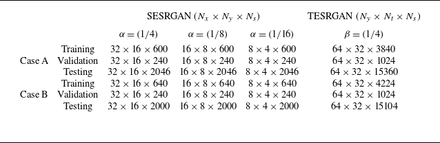
. The dataset used for cases A and B in the transfer learning is summarised in table 2. For the SESRGAN transfer learning, the number of training samples
 $N_s$
is reduced by more than half, while for TESRGAN,
 $N_s$
is reduced by nearly two thirds. Additionally, the number of epochs is decreased to 200 and 100 for SESRGAN and TESRGAN training, respectively, which significantly reduces the training time and computational cost.
Summary of dataset configurations for transfer learning of cases A and B.

Figures 17(c) and 17(d) present the SR reconstruction results of
 $U^*$
and
 $V^*$
after applying transfer learning. It is evident that the reconstruction accuracy is significantly improved compared with the original model. For case A, the instantaneous velocity fields at all SR factors are successfully recovered, showing excellent agreement with the PIV reference in both components. In contrast, for case B, while the
 $\times$
4 and
 $\times$
8 SR reconstructions achieve good accuracy, the
 $\times$
16 case still exhibits noticeable errors. These discrepancies primarily manifest as overestimations in the amplitude of both velocity components.
Comparison of MSE
 $\epsilon$
between the original model and transfer-trained model for (a) case A and (b) case B, showing results of the
 $U^*$
component at different SR factors.

The reconstruction MSE errors of the original and transfer-trained models for cases A and B are compared in figure 18, where only the
 $U^*$
component errors are presented due to the similar trends observed in
 $V^*$
. It is evident that transfer learning substantially reduces
 $\epsilon$
at all SR factors. For example, in the
 $\times$
4 case,
 $\epsilon$
is reduced by more than four times compared with the original model. As the SR factor increases, the reduction in
 $\epsilon$
also becomes more pronounced, highlighting the effectiveness of transfer learning in improving reconstruction accuracy under challenging downsampling conditions. Overall,
 $\epsilon$
in case B is consistently higher than that in case A, which can be attributed to the fundamentally different vortex evolution dynamics in case B compared with the baseline condition. Interestingly, the
 $\epsilon$
values of case A after transfer learning are even lower than those of the original model applied to the baseline condition (
 $f_m = 20$
Hz), as shown in figure 9(a). A detailed comparison between the transfer-trained model reconstructions and the reference PIV results is provided in Appendix B. The results indicate that the GAN-based model with transfer learning achieves excellent generalisation for recovering fluctuation parts in flows with similar dynamics, supporting substantial flow data enhancement. However, for case B with a different vortex dynamics, accurate reconstruction is only achieved at
 $\times$
4 and
 $\times$
8 SR factors. Therefore, it is expected that the combination of GAN-based approaches and transfer learning can reliably achieve at least
 $\times$
8 SR for flows with varying vortex dynamics.
3.5. Efficiency and limitation of GAN-based spatio-temporal super-resolution
To evaluate the efficiency improvements enabled by the GAN-based spatio-temporal SR model for accelerating PIV raw particle image-to-velocity field analyses, the training times of both the original and transfer-trained SESRGAN and TESRGAN models are critical. Figure 19 illustrates the evolution of the generator loss
 $\mathcal{L}_{G}$
over training epochs. For the original SESRGAN models (figure 19
a), higher SR factors require more epochs for
 $G$
to sufficiently optimise parameters and generate high-fidelity HR velocity fields, with convergence generally achieved after approximately 300 epochs. After convergence,
 $\mathcal{L}_{G}$
stabilises, indicating robust training. During transfer learning for cases A and B, the pre-trained original model serves as a strong initialisation, significantly accelerating convergence. Case A (with a vortex dynamics similar to the baseline) converges faster than case B (with a distinct vortex dynamics). Nevertheless, all transfer-trained SESRGAN models achieve stable convergence within 200 epochs. For TESRGAN training (figure 19
b), since the temporal downsampling factor
 $\beta$
remains fixed at (1/4), all original models converge in approximately 100 epochs, while the transfer-trained TESRGAN models achieve convergence even faster, within approximately 50 epochs.
Evolution of generator loss
 $\mathcal{L}_{G}$
during training: (a) SESRGAN models and (b) TESRGAN models.

Based on § 3.4, it is demonstrated that the proposed model can maintain good generalisation capability at an
 $\times$
8 SR factor even under different vortex dynamics, accurately reconstructing spatio-temporal SR flow fields. Therefore, the following analysis on improving PIV analysis efficiency focuses on the
 $\times$
8 case. To ensure convergence with different SR factors, the maximum training epochs are set to 800 and 200 for the SESRGAN original and transfer learning models, and 300 and 100 for the TESRGAN original and transfer learning models, respectively. Their corresponding training times per epoch are denoted as
 $t_{S,O}$
,
 $t_{S,{\textit{TL}}}$
,
 $t_{T,O}$
and
 $t_{T,{\textit{TL}}}$
. The combined SESRGAN and TESRGAN models enable the generation of HR velocity fields from LR inputs, with the reconstruction time per frame denoted as
 $t_{\textit{GAN},\textit{HR}}$
. Additionally, the processing times of the adaptive PIV algorithm in DynamicStudio 2015a under different minimum IAs are evaluated, including the commonly used
 $16 \times 16$
(Zong & Kotsonis Reference Zong and Kotsonis2018; Dong et al. Reference Dong, Zhang, Ren, Yang, Xiao, Yao and Mao2025) and their
 $\times$
8 downsampled counterparts (128
 $\times$
128), as well as 32
 $\times$
32 (Yilmaz & Rockwell Reference Yilmaz and Rockwell2012; Yu & Bernal Reference Yu and Bernal2017; Mishra & Panigrahi Reference Mishra and Panigrahi2025) and their
 $\times$
8 downsampled counterparts (256
 $\,\times\,$
256). The analysis time per frame for HR PIV is denoted as
 $t_{\textit{HR}}$
and that for LR PIV as
 $t_{\textit{LR}}$
. Specific timing details are provided in table 3. Thus, the theoretical net saved time when applying the GAN-based spatio-temporal SR model to PIV analysis is estimated as
 \begin{align} t_{\textit{net}} &= \underbrace {t_{\textit{HR}} \times N_t}_{\text{PIV HR analysis time}} - \underbrace {t_{\textit{LR}} \times N_t}_{\text{PIV LR analysis time}} - \underbrace {\left [N_O \times t_{\textit{HR}} + (N_c - 1) \times N_{\textit{TL}} \times t_{\textit{HR}}\right ]}_{\text{PIV HR analysis time for training}} \nonumber\\&\quad - \underbrace {\left [t_{S,O} + t_{T,O} + (N_c - 1) \times t_{S,\textit{TL}} + (N_c - 1) \times t_{T,\textit{TL}}\right ]}_{\text{Model training time}} \nonumber\\&\quad - \underbrace {\left [N_t - N_O - (N_c - 1) \times N_{\textit{TL}}\right ] \times t_{\textit{GAN},\textit{HR}}}_{\text{GAN-based HR reconstruction time}}. \end{align}
Here,
 $N_c$
the number of flow conditions,
 $N_O$
the number of HR PIV frames used to train the original model (1728, as shown in table 1) and
 $N_{\textit{TL}}$
the number of HR PIV frames used for transfer learning (approximately 860, as shown in table 2). It should be noted that
 $t_{\textit{net}}$
represents a theoretical estimate. Practical factors, such as additional operating time required when performing both high- and LR analyses on the same condition, as well as delays from cumulative data processing in multiple measurements, are not considered here.
Summary of PIV analysis and model training times.

Figure 20 illustrates the estimated net saved time
 $t_{\textit{net}}$
achievable using the GAN-based
 $\times$
8 SR models under different numbers of flow conditions
 $N_c$
and total PIV frames
 $N_t$
. Figure 20(a) corresponds to results reconstructed to PIV resolution with IA =
 $16 \times 16$
while figure 20(b) to IA =
 $32 \times 32$
. The cyan line indicates
 $t_{\textit{net}} = 0$
, above which the SR model yields positive time savings and below which it results in negative time savings. The blank region at the bottom denotes where the number of PIV frames is insufficient to support model training, thus making the SR approach inapplicable. It can be observed that achieving significant time benefits from the SR model requires a large
 $N_t$
and these benefits diminish as
 $N_c$
increases due to additional time costs introduced by transfer learning for each new condition. Moreover, increasing the flow field resolution demand, for example, by reducing IA from
 $32 \times 32$
to
 $16 \times 16$
, nearly doubles the time savings under the same
 $N_t$
and
 $N_c$
. For example, the plasma-induced vortices data used in this work in fact involve six conditions with a total of 17 280 PIV frames. Applying the GAN-based SR model to these data results in negative time savings for both IA =
 $16 \times 16$
and IA =
 $32 \times 32$
cases, due to the relatively small number of frames per condition. In contrast, in our earlier investigation of vortex dynamics around a pitching flat plate (Dong et al. Reference Dong, Choi, Mao and Wang2022a
), four pitching conditions were measured, each with 32 planar PIV slices, resulting in a total of 1450 000 PIV particle images. HR PIV analysis with IA =
 $16 \times 16$
would require approximately 12 179 704 s (
 $\sim$
141 days) and with IA =
 $32 \times 32$
, approximately 7829 810 s (
 $\sim$
91 days), making it impractical to process all frames. If combined with the proposed SR model, the estimated time savings are approximately 5277 874 s (
 $\sim$
61 days) for IA =
 $16 \times 16$
and 2651 650 s (
 $\sim$
31 days) for IA =
 $32 \times 32$
. These savings make it feasible to analyse the entire instantaneous flow field dataset, thereby enabling a more comprehensive understanding of detailed vortex evolution mechanisms.
Estimated net saved time
 $t_{\textit{net}}$
when applying GAN-based
 $\times$
8 SR models for different numbers of flow conditions
 $N_c$
and total PIV frames
 $N_t$
: (a) IA =
 $16 \times 16$
and (b) IA =
 $32 \times 32$
, where the cyan line indicates the zero-savings boundary (
 $t_{\textit{net}} = 0$
). The hollow star marker denotes the application of the SR model on the plasma-induced velocity field analysis, while the filled star marker indicates the application on the pitching flat plate analysis (Dong et al. Reference Dong, Choi, Mao and Wang2022a
).

Spatio-temporal autocorrelation functions for different
 $y^*$
locations at
 $x^* = 5$
: (a) streamwise velocity autocorrelation
 $\rho _{uu}$
and (b) vertical velocity autocorrelation
 $\rho _{vv}$
.

The application of GAN-based SR models for accelerating PIV particle image analysis has been discussed above. In fact, not only the SR factors
 $\times$
4,
 $\times$
8 and
 $\times$
16 presented here have been tested, but higher factors such as
 $\times$
32 and
 $\times$
64 were also attempted. However, at these higher factors, the model fails to converge and cannot generate physically realistic reconstruction results. Furthermore, we observed that while the model can achieve up to
 $\times$
16 spatial SR, it is only able to realise
 $\times$
4 temporal SR; attempts at
 $\times$
8 and
 $\times$
16 temporal SR failed to converge. This limitation is considered to stem from changes in data correlation. To verify this, autocorrelation functions are employed to quantify spatio-temporal data coherence, as illustrated in figure 21. The spatial autocorrelation for the streamwise component is defined as
 \begin{equation} \begin{aligned} \rho _{uu}(\triangle x^*/\alpha ) = \frac {\langle u(x^*) u(x^* + \triangle x^*/\alpha ) \rangle }{\langle u(x^*) u(x^*) \rangle }, \end{aligned} \end{equation}
and the temporal autocorrelation as
 \begin{equation} \begin{aligned} \rho _{uu}(\triangle \tau ^*/\beta ) = \frac {\langle u(\tau ^*) u(\tau ^* + \triangle \tau ^*/\beta ) \rangle }{\langle u(\tau ^*) u(\tau ^*) \rangle }, \end{aligned} \end{equation}
where
 $\triangle x^*$
and
 $\triangle \tau ^*$
represent the spatial gap and temporal interval of the HR PIV data, respectively. The same definitions apply to
 $\rho _{vv}$
. It is observed that
 $\rho _{uu}$
decays more slowly with increasing spatial downsampling factor than with temporal downsampling and maintains higher values even at large downsampling factors. In contrast,
 $\rho _{vv}$
exhibits a more rapid decay in both spatial and temporal directions, reflecting weaker intrinsic coherence. Considering that the plasma jet flow is dominated by the
 $U^*$
component, the degradation in
 $\rho _{uu}$
is identified as the primary factor limiting the achievable SR factor. For temporal SR, training data are constructed by sampling instantaneous velocity fields at the same
 $x^*$
position but at different
 $\tau ^*$
instants (see § 2.3). From a Lagrangian perspective, fluids at
 $\tau ^*$
have already convected downstream by
 $\tau ^*+\triangle \tau ^*/\beta$
, thus reducing data correlation in the
 $y^*-\tau ^*$
plane and then hindering model convergence. Therefore, when designing GAN-based SR models, it is crucial to consider the inherent convection and spatio-temporal coherence of the flow, as these factors directly affect data correlation and set the fundamental limits on achievable SR factors.
4. Conclusions
Two GAN-based models are sequentially trained in spatial and temporal domains to achieve spatio-temporal SR reconstruction of plasma-induced vortex flows captured by PIV, including the formation, growth, transition and breakdown stages. The reconstruction performance is quantitatively and qualitatively evaluated against HR PIV reference data under time-averaged, instantaneous and phase-averaged conditions. The results show that the GAN-based models successfully reconstruct high-fidelity HR flow fields from multiple LR inputs at varying SR factors. However, reconstruction accuracy decreases as the SR factor increases. For temporal SR, an increased time interval between LR input frames leads to greater reconstruction errors due to reduced temporal velocity correlation.
For time-averaged flows, the models consistently reconstruct key plasma jet characteristics, such as plasma thrust and the self-similar vertical velocities, at all SR factors due to the suppressed fluctuation information. For instantaneous fields, the models effectively recover velocity fluctuations and small-scale vortical structures at SR factors of
 $\times$
4 and
 $\times$
8, enabling accurate capture of dominant POD modes and phase evolution. In contrast, at
 $\times$
16, the reconstruction of small-scale features becomes limited due to the highly downsampled inputs, introducing noticeable errors and restricting reconstruction primarily to large-scale structures. In phase-averaged fields, both primary and secondary vortices are accurately reconstructed at
 $\times$
4 and
 $\times$
8 over all phases, capturing vortex centroid, radius, and circulation. At
 $\times$
16, however, accurate reconstruction is limited to primary vortices within the range of
 $\phi = 60^\circ$
to
 $300^\circ$
, where early-stage small vortices (
 $\phi \lt 60^\circ$
) are overestimated and post-breakdown diffuse structures (
 $\phi \gt 300^\circ$
) tend to be underestimated.
To evaluate model generalisability, transfer learning is applied to cases A and B, which exhibit similar and distinct vortex dynamics, respectively. By fine tuning only the generator’s SR layers using a small number of samples, the models achieve significantly improved reconstruction accuracy on unseen flow conditions. In particular, for case A at
 $\times$
16, the transferred model surpasses the baseline performance, accurately recovering plasma thrust and vortex circulation. These findings demonstrate that combining GANs with transfer learning enables reliable spatio-temporal SR reconstruction at factors of at least
 $\times$
8 with diverse flow fields. Therefore, the model’s potential for accelerating PIV particle-to-velocity analysis under
 $\times$
8 SR is further assessed. Significant efficiency gains are observed for large PIV frames, such as the pitching flat plate measurements by Dong et al. (Reference Dong, Choi, Mao and Wang2022a
), while the benefit diminishes as the number of test conditions increases due to the added cost of transfer learning. Reducing the minimum IA (e.g. from 32
 $\times$
32 to 16
 $\times$
16) yields a twofold increase in net time savings during analysis. Finally, the achievable SR factor is found to depend on the spatio-temporal coherence of the flow, where a rapid decay in autocorrelation limits further SR enhancement.
Acknowledgements
The authors thank Professor K.-S. Choi for supporting the experimental measurements and Professor J. Yao for providing the DNS data of the turbulent channel flow. The authors also acknowledge the High-Performance Computing Centre of Yangtze Delta Region Academy in Jiaxing for supporting the computational resources for model training.
Funding
This work was jointly supported by the National Natural Science Foundation of China (Grant Nos. 12302367 and 12202059), the Zhejiang Provincial Natural Science Foundation of China (Grant No. LQ24A020013) and the China Postdoctoral Science Foundation (Grant No. 2024M754111).
Declaration of interests
The authors report no conflict of interest.
Appendix A. Spatio-temporal reconstruction of turbulent channel flow
To further assess the performance of the proposed model under different flow conditions, DNS data of rectangular turbulent channel flow are considered. The simulation is carried out using an in-house code (Yao, Chen & Hussain Reference Yao, Chen and Hussain2022), with periodic boundary conditions imposed in the streamwise (
 $x$
) and spanwise (
 $z$
) directions. The channel flow Reynolds number is
 $Re_\tau = 110$
and the computational domain is
 $2\pi h \times 2h \times \pi h$
. At each time step, a velocity field of size
 $96 \times 96 \times 96$
is generated. Data on the two-dimensional
 $x$
–
 $y$
plane at
 $z = 0.5\pi h$
, covering
 $x = 0$
–
 $2\pi h$
and
 $y = -0.8h$
–
 $0.8h$
, are extracted for GAN-based model training, resulting in a dataset with
 $N_x \times N_y \times N_t = 96 \times 64 \times 3279$
. Averaging pooling is subsequently employed to produce downsampled LR data at different scales. Finally, the dataset is divided into training, validation, and testing subsets, with the detailed information provided in table 4. It is noted that
 $x^*$
and
 $y^*$
in this appendix denote the normalised coordinates
 $x/h$
and
 $y/h$
, respectively.
Summary of dataset configurations of turbulent channel flow for SESRGAN and TESRGAN training.

Reconstructed streamwise velocity fields
 $U^*$
of turbulent channel flow at SR factors of (a)
 $\times$
4, (b)
 $\times$
8 and (c)
 $\times$
16 (left), with the corresponding absolute error maps relative to DNS (right). The reference DNS field is shown at the top.

Comparison of reconstructed and DNS instantaneous velocities over 1000 time steps at different streamwise locations for (a)
 $x^* = 0.5 \pi$
and (b)
 $x^* = 1.5 \pi$
. The left and right columns correspond to the streamwise velocity
 $U^*$
and the vertical velocity
 $V^*$
, respectively. The sampling location in the flow field is indicated at the top.

Figure 22 compares the reconstructed streamwise velocity fields with the reference DNS result for turbulent channel flow at
 $t U_b/h$
= 2200, where
 $U_b$
is the bulk velocity of the channel. The left column shows the reconstructed velocity fields, while the right column presents the maps of absolute error between the reconstructions and the DNS. All cases are able to reconstruct the turbulent channel flow with reasonable accuracy, yet the reconstruction error clearly increases with the SR factor. For the
 $\times$
4 case, the reconstructed field agrees closely with the DNS, with only minor discrepancies. For the
 $\times$
8 case, pronounced errors are primarily observed near the channel walls (
 $y^* \gt \pm 0.5$
). For the
 $\times$
16 case, the error grows substantially, with additional deviations appearing at the channel centre (
 $y^* = 0$
). This behaviour is similar to plasma-induced flows, where high downsampling leads to the loss of small-scale information, thereby limiting reconstruction accuracy.
Figure 23 presents a comparison of the reconstructed instantaneous velocities with the reference DNS over 1000 time steps at selected sampling points, whose locations are shown at the top. The time series of
 $U^*$
demonstrates that the reconstructions can capture the dominant temporal fluctuations for all SR factors. At
 $y^* = \pm 0.5$
, where near-wall dynamics are more energetic, the
 $\times$
4 and
 $\times$
8 cases exhibit close agreement with the DNS, while the
 $\times$
16 case shows modest deviations in amplitude during intermittent bursts. At the channel centre (
 $y^* = 0$
), the temporal evolution remains well reproduced, although the
 $\times$
16 case displays slightly damped fluctuations. For
 $V^*$
, which is more sensitive to small-scale motions and cross-stream interactions, the agreement remains satisfactory at
 $\times$
4 and
 $\times$
8, whereas the
 $\times$
16 case again shows larger departures, particularly in capturing sharp temporal variations. These deviations highlight the increasing difficulty of accurately recovering the transverse dynamics under strong downsampling.
Appendix B. Spatio-temporal reconstruction of cases A and B using transfer learning
Figure 24 compares the instantaneous streamwise and vertical velocity peaks obtained from the model reconstructed and the PIV reference data for cases A and B. For case A (figure 24
a), the reconstructed peak velocities show excellent agreement with the PIV reference at all SR factors. The high-density regions remain closely clustered along the diagonal line, indicating that both the distribution and amplitude of the reconstructed velocities are well preserved. Compared with the baseline results shown in figure 8(c), the
 $\times$
16 reconstruction in case A exhibits much tighter clustering, indicating enhanced reconstruction accuracy at this high downsampling level. This highlights the excellent adaptability and robustness of the transfer-trained model when applied to flow fields with a dynamics similar to the original training data. In contrast, for case B (figure 24
b), the
 $\times$
4 and
 $\times$
8 SR reconstructions show reasonable agreement with the PIV reference, though the clustering is slightly more dispersed than in case A, reflecting the greater difficulty in capturing the more complex vortex dynamics. At
 $\times$
16, the peak velocities exhibit a pronounced spread and clear upward deviations from the diagonal, indicating reduced reconstruction accuracy.
Comparison of instantaneous streamwise and vertical velocity peaks obtained from the transfer-trained model and PIV reference data at different SR factors: (a) case A and (b) case B.

Quantitative comparison of reconstructed flow fields with PIV reference data for cases A and B after transfer learning: (a) streamwise evolution of maximum velocity
 $U_m$
of the time-averaged plasma jet, (b) plasma thrust per unit width
 $M_x$
of the time-averaged plasma jet, (c) phase-averaged trailing vortex radius
 $r_c$
and (d) phase-averaged trailing vortex circulation
 $\varGamma _c$
.

Similar results are also observed in the Reynolds stress fields and the time coefficients of the POD modes, which are not shown here, further confirming that the model’s generalisation capability can be substantially enhanced through transfer learning with a limited number of additional samples. For flow conditions with a vortex dynamics similar to the baseline, such as case A, the transfer-trained model achieves even better reconstruction performance than the original baseline model, particularly in the highly challenging
 $\times$
16 SR. For flow conditions with a different vortex dynamics, such as case B, the model still demonstrates good reconstruction accuracy at
 $\times$
4 and
 $\times$
8, but its performance at the highly downsampled
 $\times$
16 factor remains limited and requires further improvement.
To quantitatively evaluate the reconstruction capability of the transfer-trained model, the time-averaged streamwise maximum jet velocity
 $U_m$
, plasma thrust per unit width
 $M_x$
and the phase-averaged vortex radius
 $r_c$
and circulation
 $\varGamma _c$
are calculated and shown in figure 25. Note that for case B, due to the formation of vortex pairing, the phase
 $\phi$
is divided into
 $2f_s/f_m$
. For the time-averaged results (figures 25
a and 25
b), consistent with the findings in § 3.1, both cases A and B accurately recover
 $U_m$
and
 $M_x$
at all SR factors, with nearly perfect agreement with the PIV reference data. This indicates that when considering only time-averaged flow information, the GAN-based model combined with transfer learning exhibits excellent generalisation capability, enabling up to
 $\times$
16 SR while maintaining high accuracy. This corresponds to an enhancement of approximately three orders of magnitude in flow field information (
 $(1/(\alpha \times \alpha \times \beta)) = 16 \times 16 \times 4$
) reconstructed from LR data. For the phase-averaged fields (figures 25
c and 25
d), case A with similar vortex dynamics to the baseline maintains high reconstruction accuracy for all SR factors. Notably, the
 $\times$
16 SR results even surpass the baseline model performance, as shown in figures 16(c) and 16(d).