1. Introduction
Natural flyers and swimmers are known to take advantage of external flow disturbances to reduce the cost of locomotion (Lissaman & Shollenberger Reference Lissaman and Shollenberger1970; Liao et al. Reference Liao, Beal, Lauder and Triantafyllou2003b). Meanwhile, the interaction of a wing with disturbances raises concerns in several engineering applications. Blade–vortex interactions in helicopters (Fletcher & Brown Reference Fletcher and Brown2007), wind turbines (Choudhry et al. Reference Choudhry, Mo, Arjomandi and Kelso2014; Zhao, Sheng & Afjeh Reference Zhao, Sheng and Afjeh2014; Tadokoro, Yokoyama & Iida Reference Tadokoro, Yokoyama and Iida2017) and turbomachinery (Binder et al. Reference Binder, Forster, Mach and Rogge1987) often result in noise, structural and control issues. The study of unsteady flow phenomena is often focused on wings engaged in unsteady motion in the presence of a uniform free stream. Modern pursuits in improving the design and performance of man-made propulsors and energy harvesters demand more consideration of the context of unsteady wings encountering flow disturbances. In this paper, experimental and theoretical investigations are conducted on an unsteady airfoil encountering flow disturbances generated by an external source. Particular focus is placed on the effect of the encounter on the leading-edge vortex (LEV) shedding characteristics of the airfoil.
The effect of flow interactions manifests in the performance measures such as propulsive efficiency, thrust or lift. Liao, Dong & Lu (Reference Liao, Dong and Lu2004) show that lift of an airfoil in the wake of a circular cylinder adopts the shedding frequency of the cylinder. Fish have been observed to capture energy from an oncoming vortex street through Kármán gaiting (Liao et al. Reference Liao, Beal, Lauder and Triantafyllou2003a). Detailed investigations on Kármán gaiting reveal that fish optimize the efficiency of energy extraction by altering the phase difference between their motion and the oncoming vortex street (Beal et al. Reference Beal, Hover, Triantafyllou, Liao and Lauder2006; Toming, Chambers & Kruusmaa Reference Toming, Chambers and Kruusmaa2014; Li et al. Reference Li, Yang, Xu, Wang, Wang and Xu2017). For a flapping foil encountering a vortex street, a strong dependence exists between the efficiency of the foil and the phase difference between the foil oscillation and the arrival of incident vortices (Gopalkrishnan et al. Reference Gopalkrishnan, Triantafyllou, Triantafyllou and Barrett1994; Streitlien, Triantafyllou & Triantafyllou Reference Streitlien, Triantafyllou and Triantafyllou1996). The thrust of propulsive foils (Zhang et al. Reference Zhang, Su, Yang and Wang2010; Shao & Pan Reference Shao and Pan2011) and the energy harvesting potential of flapping-foil energy harvesters (Wei & Zheng Reference Wei and Zheng2017a, Reference Wei and Zhengb) can be enhanced significantly depending on the interaction mode. The interaction mode is often classified as constructive or destructive (Li & Sun Reference Li and Sun2015) based on its effect on the performance measure under consideration. Multi-wing systems present another arena for studying such interactions where one wing encounters the disturbances generated by another one. Substantial enhancement in thrust (Muscutt, Weymouth & Ganapathisubramani Reference Muscutt, Weymouth and Ganapathisubramani2017) and energy harvesting potential (Wu, Chen & Zhao Reference Wu, Chen and Zhao2015) compared with single-wing case resulting from constructive wing–wake interaction has been observed in such arrangements.
Interesting fluid-dynamic phenomena like dynamic stall and LEV formation are often encountered in airfoils and wings performing unsteady motion. The formation and dynamics of LEV on unsteady wings have been extensively studied (Ellington et al. Reference Ellington, Van Den Berg, Willmott and Thomas1996; Wang & Eldredge Reference Wang and Eldredge2013; Ramesh et al. Reference Ramesh, Gopalarathnam, Granlund, Ol and Edwards2014) and are well known to be responsible for lift augmentation in flapping flight (Dickinson, Lehmann & Sane Reference Dickinson, Lehmann and Sane1999; Shyy et al. Reference Shyy, Aono, Chimakurthi, Trizila, Kang, Cesnik and Liu2010; Pitt Ford & Babinsky Reference Pitt Ford and Babinsky2013). While early works like that of Jefferies & Rockwell (Reference Jefferies and Rockwell1996) have reported the observations of LEV shedding characteristics of airfoils being altered by external flow disturbances, recent research efforts using high-fidelity numerical studies and advanced experimental techniques have attempted to take a detailed look into the mechanisms governing the interaction phenomena. In an experimental study on a tandem wing configuration, Rival, Manejev & Tropea (Reference Rival, Manejev and Tropea2010) observed that vortex-induced separation can lead to the formation of an LEV on the downstream wing, and associated the cause with the upwash generated at the leading edge by the vortices shed from the upstream wing. A numerical study by Wei & Zheng (Reference Wei and Zheng2017a) reveals that the susceptibility to LEV formation or suppression of an unsteady airfoil in the presence of an oncoming vortex street can be correlated to the pattern of pressure distributions and adverse pressure gradients arising from the interactions. While experimental and high-fidelity computational fluid dynamics (CFD) methods facilitate detailed study of flow phenomena, low-order theoretical models augment these methods by providing an intuitive approach to understanding the flow physics from a fundamental perspective and equipping us with the insight to predict various trends. The seminal theoretical modelling works by Wagner (Reference Wagner1925), Theodorsen (Reference Theodorsen1935), Küssner (Reference Küssner1936), von Kármán & Sears (Reference von Kármán and Sears1938) and Sears (Reference Sears1941) have proven invaluable to the field of unsteady aerodynamics despite the assumptions of small-amplitude motions, planar wakes and attached flows. The desire for expanded applicability of unsteady potential-flow methods has long motivated inviscid modelling approaches such as those by McCune, Lam & Scott (Reference McCune, Lam and Scott1990), Wang & Eldredge (Reference Wang and Eldredge2013) and Ramesh et al. (Reference Ramesh, Gopalarathnam, Granlund, Ol and Edwards2014) that can perform regardless of amplitude and reduced frequency of motion, and impose no restrictions on the trailing-wake dynamics. Alaminos-Quesada & Fernandez-Feria (Reference Alaminos-Quesada and Fernandez-Feria2017) use potential-flow theory to analyse the effect of the angle of attack on the interaction of a two-dimensional vortex with a flat plate. Wei & Zheng (Reference Wei and Zheng2017a) present an approach to explain the formation of LEVs based on pressure distributions and adverse-pressure-gradient patterns using a simple theoretical model. Theoretical approaches to predict the interactions between external flow disturbances and unsteady airfoils with LEV shedding still need consideration.
Recently, Ramesh et al. (Reference Ramesh, Gopalarathnam, Granlund, Ol and Edwards2014) presented a potential-flow-based approach to determine the initiation, growth and termination of leading-edge vorticity from airfoils engaged in arbitrary unsteady motions based on the critical value of suction at the leading edge. In this phenomenologically augmented method, a single empirical parameter – the critical value of the leading-edge suction parameter (LESP) – unifies all the kinematic factors of the airfoil in determining its LEV shedding characteristics. This concept also eliminates the use of commonly used ad hoc criteria such as the start and stop of LEV shedding based on a local angle of attack or the assumption of continuous shedding, and has a broader scope of application than semi-empirical methods that can only be employed for limited situations. A discrete-vortex implementation of this approach, called the LESP-modulated discrete-vortex method (LDVM), has been extensively validated for several case studies by Ramesh et al. (Reference Ramesh, Gopalarathnam, Granlund, Ol and Edwards2014).
In this paper, we use experimental methods and theoretical tools based on LDVM and LESP to study the unsteady flow interactions and their effects on the lift of an airfoil undergoing high-amplitude pitching motions in the presence of oncoming disturbances. The periodic disturbances are systematically generated in the experiments as a von Kármán street using a sinusoidally rotating circular cylinder placed upstream of the airfoil. The complex flow interactions are observed qualitatively using particle-image velocimetry (PIV) and analysed in detail using finite-time Lyapunov exponent (FTLE) techniques. The experimental set-up used for this study is described in § 2. With the confidence gained from the previous success of the LDVM method and the LESP concept, the LDVM framework is extended in § 3 to obtain a low-order model that incorporates the effects of the encounter of an unsteady airfoil with external flow disturbances. The disturbance model is initially informed by results from experiments on a static airfoil and is then used for predictions of unsteady airfoils. Some theoretical tools based on LESP are derived in § 4. These tools are used hand-in-hand with experimental results in § 5 to gain insight into the effect of the disturbances on the LEV shedding characteristics and associated loads of the airfoil. Finally, the conclusions are discussed in § 6.
2. Experimental set-up
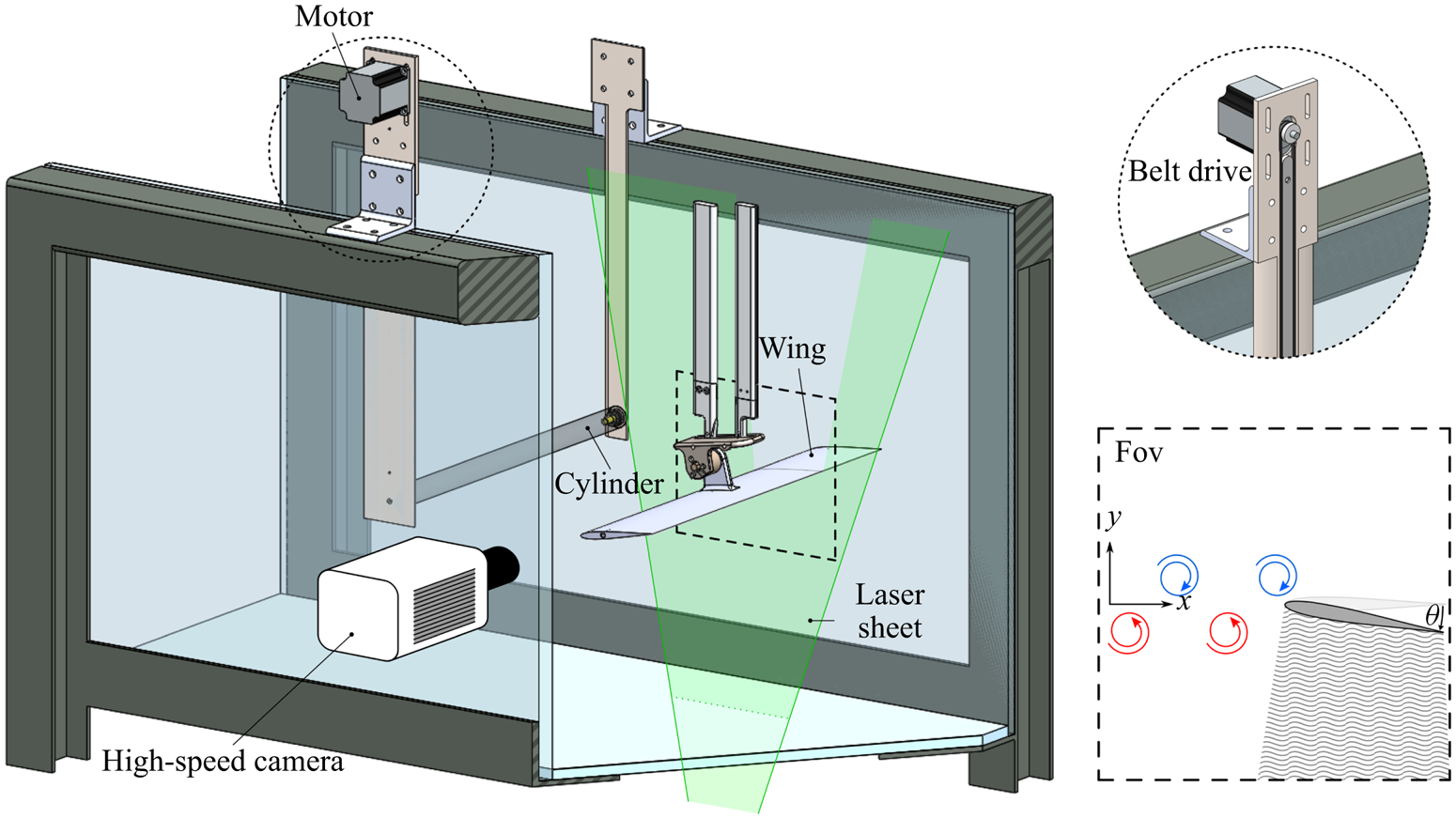
The effect of external flow disturbances on the aerodynamic loading and vortex-shedding characteristics of an unsteady airfoil is examined experimentally under the influence of disturbances generated systematically using an upstream circular cylinder. The cylinder–airfoil arrangement is illustrated in figure 1. The experiments are performed in the US Air Force Research Laboratory's horizontal free-surface water tunnel. The tunnel has 4 : 1 contraction and a 46 cm wide by 61 cm high test section with an operational speed range of  $3 - 105\ \textrm {cm}\ \textrm {s}^{-1}$ and a free-stream component of turbulence intensity of 0.4 % at
 $5 - 40\ \textrm {cm}\ \textrm {s}^{-1}$. The tunnel is outfitted with a three degree of freedom motion rig, consisting of a triplet of H2W linear motors, driven by AMC DigiFlex servo-drives controlled by a Galil DMC 4040 4-channel card, with user-selected proportional/integral/derivative constants for each channel. This allows for the pitching, plunging and surging of test articles. Direct force measurement is conducted via an ATI NANO-25 IP68 six-component force balance. Measurements are sampled at a rate of
 $1\ \mathrm {kHz}$ and treated with a Chebyshev 2 low-pass filter with a cutoff frequency of
 $16\ \mathrm {Hz}$. All the force measurements are ensemble averaged over 10 runs.
Schematic of the experimental set-up showing the airfoil subjected to periodic flow disturbances generated by the upstream circular cylinder.

2.1. Test geometries
In this study, a symmetric version of the SD7003 airfoil is chosen for the wing geometry so as to eliminate the effects of camber and isolate the effects of the flow disturbances on the aerodynamics of the airfoil. The symmetric airfoil is derived from the SD7003 airfoil by a modification of the airfoil profile to a zero-camber configuration while preserving the airfoil thickness distribution along the chord. This approach maintains the leading-edge curvature of the airfoil, thus nominally maintaining the Reynolds-number-specific critical-LESP value (and thus the LEV-shedding characteristics, as explained later in § 5.1) previously determined by Ramesh et al. (Reference Ramesh, Gopalarathnam, Granlund, Ol and Edwards2014) for the SD7003 airfoil. The wing model used in the experiments is fabricated from plastic (VeroWhite) through additive manufacturing and is reinforced with a spanwise carbon-fibre rod insert. The wing chord length of the model is  $c=10.16$ cm.
The cylinder has a diameter,  $d$, of 2.54 cm and a length, L, such that the aspect ratio,
 $L/d$, is 18. The axis of the cylinder is oriented normal to the tunnel walls, parallel to the wing leading edge. Both the wing and the cylinder span the width of the test section to produce a nominally two-dimensional flow field. Experiments were conducted at a free-stream speed of
 $U_{\infty }=29.6\ \textrm {cm}\ \textrm {s}^{-1}$, corresponding to a diameter-based Reynolds number of
 $Re_d=7500$ and a chord-based Reynolds number of
 $Re_c=3 \times 10^{4}$. The wing has a minor gap of
 ${\sim }0.5$ mm existing at the wing–wall interface at both ends of its span. The cylinder is supported at the tunnel walls via low-profile vertical plate inserts.
The cylinder generates a periodic disturbance to be encountered by the downstream wing in the form of a von Kármán vortex street with a natural shedding frequency,  $f$, corresponding to a Strouhal number of
 $St=fd/U_{\infty }=0.2$. With a chord-to-diameter ratio of
 $c/d=4$, the resulting street of vortices is comparable in size to LEVs of the wing in dynamic stall. The wing is positioned downstream of the cylinder at a distance of
 $x/d=8$, measured from the cylinder centre to the wing leading edge. This spacing is selected to ensure that the presence of the wing does not alter the natural shedding dynamics of the cylinder. The set-up allows for various vertical positions of the wing relative to the cylinder centreline. In this paper, we focus on the cases where the airfoil performs pitching motions about a pivot point that coincides with the centreline of
 $y/d=0$.
2.2. Flow visualization
Two-dimensional time-resolved PIV measurements were performed using the experimental set-up illustrated in figure 2. The water tunnel was seeded with polyamide particles of  $60\ \mathrm {\mu }\mathrm {m}$-diameter (LaVision,
 $\textrm {SG}=1.03$) and illumination was provided by an Nd:YLF laser sheet (Photonics Industries DM50-527,
 $50\ \textrm {mJ}\ \textrm {pulse}^{-1}$, 10 kHz max) oriented in the streamwise direction and positioned at the three-quarter span of the wing. Images were recorded by high-speed camera (PCO Dimax S4, 4MP, 1279 f.p.s. at max resolution). The velocity vectors were calculated using Fluere version 1.3. Two passes of interrogation areas, with initial and final sizes of
 $64\ \textrm {px}^{2}$ and
 $32\ \textrm {px}^{2}$, respectively, were used to determine the particle displacements from single-frame images sampled at 350 Hz. An interrogation area overlap of 50 % was used. The resultant vector fields contained
 $123 \times 123$ vectors with a resolution of
 $(x/d, y/d)=(0.074, 0.074)$. Instantaneous vector fields were phase averaged using snapshot proper orthogonal decomposition (POD) (Perrin et al. Reference Perrin, Braza, Cid, Cazin, Barthet, Sevrain, Mockett and Thiele2007) for the cylinder-only cases. For the studies of the airfoil in the cylinder wake, the PIV data were ensemble averaged over consecutive runs of the experiment. A programmed trigger was used to ensure that all the runs were synchronized.
Experimental set-up: direct force measurement and flow visualization using time-resolved PIV.

2.3. Control of the disturbance phasing
The focus of this work is the effect of the upstream disturbances generated by the cylinder on the dynamic wing positioned downstream. Critical to this effort is the capability to control the phase of the proximal vortical disturbances relative to the wing's kinematic commencement. Previous works (Okajima, Takata & Asanuma Reference Okajima, Takata and Asanuma1975; Cheng, Liu & Lam Reference Cheng, Liu and Lam2001; Rockwood & Medina Reference Rockwood and Medina2020) have shown that phase control of the periodic wake can be achieved by rotational oscillation of the cylinder about its axis. To this end, a timing belt was integrated flush into one of the vertical plates to provide rotary motion to the cylinder about its respective axial coordinate via a stepper motor, as illustrated in figure 2. The cylinder is driven in a sinusoidal angular profile of rotational amplitude  $45^{\circ}$. The angular frequency,
 $\omega$, corresponds to the natural shedding frequency of the cylinder and thus to a Strouhal number of
 $St=0.2$.
The commanded cylinder rotation,  $\psi _c$, is given by
 \begin{equation} \psi_c(t) = \psi_{c.max} \sin(\omega t + \varTheta), \end{equation}
in which the cylinder-oscillation phase,  $\varTheta$, is set to achieve a desired relative position of the oncoming vortices with respect to the wing leading edge at a particular instant in time. The result is a commanded phase,
 $\phi$, of the vortical disturbance with respect to the wing's position and kinematic timing. The phasing convention, illustrated in figure 3, corresponds to the relative position of the vortical disturbances with respect to the wing leading edge.
(a) Definition of the phase  $\phi$ based on the position of the oncoming vortical disturbances relative to the airfoil. (b) Demonstration of the control of
 $\phi$. Lift-coefficient histories of a static airfoil at zero incidence for different values of
 $\phi$ exhibiting a phase shift equal to
 $\phi$.

For a static wing,  $\phi =0^{\circ }$ is defined as the case when a clockwise vortex is coincident with the streamwise location of the leading edge at a reference point in time. The case where a counter-clockwise vortex is encountered by the leading edge at the same time corresponds to
 $\phi =180^{\circ }$. Figure 3 also demonstrates the effective phase control enabled by active shedding of the rotating cylinder for a static airfoil placed in the flow centreline at
 $y/d=0$ at zero incidence. For this configuration, the von Kármán street emanating from the cylinder is bisected by the wing. Lift histories for various values of
 $\phi$, 90 degrees apart, showcase a phase differential of
 $90$ degree increments as intended. For a dynamic wing,
 $\phi$ is similarly defined based on the location of the vortices at the start of the wing's prescribed kinematic profile. Different disturbance configurations (corresponding to different values of
 $\phi$) can be achieved at the initiation of motion by changing the cylinder-rotation phase
 $\varTheta$. This leads to different interaction modes between the wing and the oncoming disturbances, as visualized and discussed in detail later in § 5.
Another benefit of using the rotating cylinder is that the rotating cylinder preserves the spatial layout of the wake shed by a static cylinder but reduces spurious cycle-to-cycle variation in the shedding pattern. In cylinder wakes the two most energetic modes are associated with the von Kármán vortices, and when their respective temporal coefficients, denoted by  $a_1$ and
 $a_2$, are normalized by their energy and plotted against each other, they produce a phase plot, an example of which is shown in figure 4(a) for the static cylinder and in figure 4(b) for the rotating cylinder. Using figure 4(a) for the discussion, each point in this figure corresponds to a velocity field at one instant in time. From this figure, a phase angle can easily be determined for each velocity field as
 $\beta =\tan ^{-1}(a_{2,normalized}/a_{1,normalized})$. In this study the phase plot was divided equally into 36 bins, each 10 degrees wide. A total of 4000 velocity fields were used, which encompassed 55 periods of von Kármán vortex shedding. Each velocity field was placed in the corresponding bin based on its phase angle, and then all velocity fields within each bin were averaged together to form phase-averaged velocity fields. Phase averaging mitigates some of the random errors derived from the PIV velocity-vector calculation. Comparison between static-cylinder and rotating-cylinder POD phase plots of figure 4 reveals significant reduction in hysteresis for the rotating cylinder. This observation translates to a reduction in cycle-to-cycle fluctuations in vortical shedding for the rotating cylinder.
POD phase plot for cylinder wakes: (a) static cylinder, (b) dynamic cylinder.

Figure 5 showcases the typical wake structure behind the rotating cylinder in contrast to the static cylinder. Note that the rotating cylinder also provides for greater vorticity concentration for a given vortical element of the vortex street. This characteristic helps to ensure that a given vortical element maintains coherency downstream at the point of wing interaction.
Phase-averaged vorticity contours of the wake: (a) static cylinder, (b) rotating cylinder.

3. Low-order aerodynamic model
The low-order modelling methodology builds upon the LESP-modulated discrete-vortex method (LDVM) developed in previous research by Ramesh et al. (Reference Ramesh, Gopalarathnam, Granlund, Ol and Edwards2014) for unsteady airfoils with intermittent LEV shedding. LDVM distils the determination of the initiation and termination of LEV shedding in unsteady airfoils to a single empirical parameter, the LESP. The backbone of this potential-flow-based discrete-vortex method is a large-angle unsteady thin-airfoil theory phenomenologically augmented using CFD or experimental information. The discrete-vortex implementation is realized as a time-stepping approach outlined by Katz & Plotkin (Reference Katz and Plotkin2000) in which the wake vorticity is modelled using discrete vortices. In the current work, the LESP concept is extended to an airfoil undergoing arbitrary unsteady motion in the presence of upstream flow disturbances generated by an external source. The essential elements of LDVM theory are briefly outlined and the theoretical background of the current approach is presented below.
3.1. Formulation
The schematic representation in figure 6 shows an airfoil of chord  $c$ undergoing arbitrary pitching and heaving kinematics in the presence of an upstream disturbance. The kinematic state of the airfoil is defined by the pitch angle
 $\theta$, the heave position
 $h$ and the respective velocities
 $\dot {\theta }$ and
 $\dot {h}$. The pivot point, located at a distance
 $x_p$ aft of the leading edge, denotes the centre of rotation of the airfoil. Also shown is a body-fixed frame
 $Bxz$, with the origin coinciding with the leading edge of the airfoil and the
 $x$ and
 $z$ axes extending in the chord-wise and chord-normal directions, respectively. The upstream disturbance is modelled using a vortical component resembling a von Kármán street superimposed on a mean component referred to here as the ‘uniform-flow speed’, denoted by
 $U$. Note that this uniform-flow speed,
 $U$, may be different from the free-stream speed of
 $U_{\infty }$ for modelling purposes to account for a velocity deficit when the airfoil is in the wake of the cylinder. The combined flow induces fluctuations in the flow velocity and the flow angle experienced by the airfoil. The wake of the airfoil consists of discrete LEVs and trailing-edge vortices (TEVs) shed from either edges of the airfoil in the previous time steps.
Illustration of the low-order framework showing the oncoming flow disturbances, the vorticity shed from the airfoil and the kinematic variables used in the theoretical formulation. Clockwise vorticity is considered positive.

The solution seeks a velocity potential,  ${\varPhi }$, that satisfies the incompressible continuity equation
 \begin{equation} \nabla^{2}{\varPhi}=0 \end{equation}
subject to the time-dependent zero-normal-flow boundary condition,
 \begin{equation} (\boldsymbol{\nabla}\boldsymbol{\varPhi}+\boldsymbol{V}_{kin})\boldsymbol{\cdot}\hat{n}=0, \end{equation}
where  $\boldsymbol {V}_{kin}$ is the relative fluid velocity experienced by the airfoil due to the airfoil kinematics (pitch and heave), and
 $\hat {n}$ is the unit normal to the local camberline of the airfoil. The velocity potential,
 $\varPhi$, consists of the unknown bound potential,
 $\varPhi _{B}$, the uniform-flow potential,
 $\varPhi _U$, the potential due to the vortical disturbances,
 $\varPhi _D$, and the wake potential potential,
 $\varPhi _{W}$, which in turn can be broken down into the velocity potential due to the discrete LEVs and TEVs
 \begin{equation} \varPhi=\varPhi_{B}+\varPhi_{U}+\varPhi_{D}+\varPhi_{W}=\varPhi_{B}+\varPhi_{U}+\varPhi_{D}+\varPhi_{LEV}+\varPhi_{TEV}. \end{equation}
The velocity potential,  $\varPhi _{D}$, due to the vortical component of the upstream disturbance, is a superposition of the potentials of two infinite rows of alternating-sign vortices of strength
 $\varGamma _k$, resembling a von Kármán street. Using the boundary condition (3.2), the unknown bound potential can be expressed in terms of the known airfoil kinematics and the free vorticity (comprising upstream vortical disturbances, LEVs and TEVs) as
 \begin{equation} \frac{\partial\varPhi_{B}}{\partial z}={-}\boldsymbol{V}_{kin}\boldsymbol{\cdot}\hat{n} -\frac{\partial}{\partial z}(\varPhi_{U}+\varPhi_D+\varPhi_{LEV}+\varPhi_{TEV}). \end{equation}
We now introduce the term downwash, denoted by  $W$, as the component of the induced velocity opposite to the normal direction, i.e. along the
 $-\hat {n}$ direction, due to uniform flow, kinematics, upstream vortical disturbances, LEVs and TEVs. We see that, to satisfy the zero-normal-flow boundary condition along the airfoil chord,
 $\partial \varPhi _B(x)/\partial z$ should be equal to
 $W(x)$ everywhere along the chord
 \begin{align} W(x,t) = \frac{\partial\varPhi_{B}}{\partial z}=\frac{\partial \eta}{\partial x}(U \cos \theta+\dot{h} \sin \theta+u_{ind}) -U \sin \theta -\dot{\theta}(x-x_p) +\dot{h} \cos \theta -w_{ind}, \end{align}
where  $\eta (x)$ is the camberline shape of the airfoil, assumed to be small in comparison with the chord length, and
 $u_{ind}(x)$ and
 $w_{ind}(x)$ are the chordwise and normal components (along positive
 $x$ and
 $z$ axes), respectively, of the velocity induced by all the free vortices along the airfoil chord
 $$\begin{gather} u_{ind}(x)=\frac{\partial \varPhi_{LEV}}{\partial x}+\frac{\partial \varPhi_{TEV}}{\partial x}+\frac{\partial \varPhi_{D}}{\partial x}, \end{gather}$$
 $$\begin{gather}w_{ind}(x)=\frac{\partial \varPhi_{LEV}}{\partial z}+\frac{\partial \varPhi_{TEV}}{\partial z}+\frac{\partial \varPhi_{D}}{\partial z}. \end{gather}$$
3.2. Solution of the flow field
Using the Glauert transformation,  $x={c}/{2}(1-\cos \nu )$, the chordwise distribution of the bound vortex-sheet strength,
 $\gamma (x,t)$, which is positive for clockwise direction, can be written in terms of
 $\nu$ as
 \begin{equation} \gamma(\nu,t)=2U_{ref}\left[A_{0}(t)\frac{1+\cos \nu}{\sin \nu} + \sum_{n=1}^{\infty}A_{n}(t) \sin(n\nu)\right], \end{equation}
where  $U_{ref}$ is the reference velocity used as a scaling parameter, the choice of which is arbitrary. This transformation boils down the solution of the flow field to obtaining the time-dependent Fourier coefficients,
 $A_{n}(t)$, from the instantaneous downwash,
 $W(x,t)$
 $$\begin{gather} A_{0}(t) ={-}\frac{1}{\rm \pi} \displaystyle \int_{0}^{\rm \pi}\frac{W(x,t)}{U_{ref}}\,\textrm{d} \nu , \end{gather}$$
 $$\begin{gather}A_{n}(t) = \frac{2}{\rm \pi} \displaystyle \int_{0}^{\rm \pi}\frac{W(x,t)}{U_{ref}} \cos (n \nu) \,\textrm{d} \nu,\quad n\geqslant 1. \end{gather}$$
The bound circulation can then be obtained by integrating  $\gamma$ as
 \begin{equation} \varGamma_B(t)= \displaystyle \int_{0}^{c}\gamma(x)\,\textrm{d} \nu={\rm \pi} c U_{{ref}}\left[A_0(t)+\frac{A_1(t)}{2}\right]. \end{equation}
In the time-stepping implementation, the wake vorticity shed from the airfoil edges are represented using discrete vortices. A newly shed vortex is placed at one-third distance between the shedding edge and the previous vortex shed from that edge. The strength of the latest-shed vortices need to be determined to obtain  $W$. At every time step a discrete TEV is released, the strength of which is obtained in accordance with Kelvin condition. At the
 $j\textrm {th}$ time step
 \begin{equation} {\rm \pi}c U_{{ref}}\left[A_0(t)+\frac{A_1(t)}{2}\right]+\varGamma_{TEV}^{j}=\varGamma_{B}^{j-1}, \end{equation}
where  $\varGamma _{TEV}^{j}$ is the unknown strength of the latest TEV and
 $\varGamma _{B}^{j-1}$ is the bound circulation of the airfoil at the previous time step. After some manipulation, we get
 \begin{equation} \varGamma_{TEV}^{j}=\frac{\varGamma_{B}^{j-1}+c\displaystyle \int_{0}^{\rm \pi} W^{0}(1-\cos\nu)\,\textrm{d} \nu} {1-c\displaystyle \int_{0}^{\rm \pi} W^{\prime}_{TEV}(1-\cos\nu)\,\textrm{d} \nu}, \end{equation}
where  $W^{\prime }_{TEV}(x)$ is the downwash distribution induced by a unit-strength discrete vortex placed at the location of the latest TEV and
 $W^{0}$ is the downwash due to all the other discrete vortices present in the flow field as well as the kinematic state of the airfoil. Ramesh et al. (Reference Ramesh, Gopalarathnam, Granlund, Ol and Edwards2014) presented a criterion to predict the initiation and termination of LEV shedding based on the maximum allowable value of suction that can be supported at the leading edge. The non-dimensional measure of the chord-parallel leading-edge suction force, called the LESP (denoted by
 $ {\mathcal {L}}$ henceforth), was shown to be associated with the leading Fourier-coefficient
 $A_0$
 \begin{equation} {\mathcal{L}}(t)=A_0(t) . \end{equation}
In LDVM, discrete LEVs are shed when  $ {\mathcal {L}}$ exceeds a critical value denoted by
 $ {\mathcal {L}}_{crit}$. The value of
 $ {\mathcal {L}}_{crit}$ for a given airfoil is largely independent of motion kinematics at a given
 $Re$. Once the value of
 $ {\mathcal {L}}_{crit}$ for a given airfoil at a given
 $Re$ is determined using experimental or CFD data, LDVM can predict the LEV shedding characteristics of that geometry for any arbitrary motion kinematics at that
 $Re$. The strengths of the LEVs are determined so as to maintain the
 $ {\mathcal {L}}$ at
 $ {\mathcal {L}}_{crit}$. Hence, when LEV shedding is active, the strengths of the LEV and TEV shed at every time step have to be determined to satisfy the Kelvin condition as well as to maintain
 $ {\mathcal {L}}$ at
 $ {\mathcal {L}}_{crit}$. This leads to a simultaneous two-variable problem in the form
 \begin{equation} [A] \begin{Bmatrix} \varGamma_{TEV} \\ \varGamma_{LEV} \end{Bmatrix} =\{B\} \end{equation}
where,
 \begin{equation} [A]= \begin{bmatrix} 1-c\displaystyle \int_{0}^{\rm \pi} W^{\prime}_{TEV}(1-\cos\nu)\,\textrm{d} \nu & 1-c \displaystyle \int_{0}^{\rm \pi} W^{\prime}_{LEV}(1-\cos\nu)\,\textrm{d} \nu \\ \displaystyle \int_{0}^{\rm \pi} W^{\prime}_{TEV}\,\textrm{d} \nu & \displaystyle \int_{0}^{\rm \pi} W^{\prime}_{LEV}\,\textrm{d} \nu \end{bmatrix} \end{equation}
and
 \begin{equation} \{B\}= \begin{Bmatrix} \varGamma_{B}^{j-1}+c\displaystyle \int_{0}^{\rm \pi} W^{0}(1-\cos\nu)\,\textrm{d} \nu\\ \displaystyle -{\rm \pi} U_{ref} {\mathcal{L}}_{crit}-\int_{0}^{\rm \pi} W^{0} \,\textrm{d} \nu \end{Bmatrix}, \end{equation}
where  $W^{\prime }_{LEV}(x)$ is the downwash distribution induced by a unit-strength discrete vortex placed at the location of the latest-shed LEV. As noted by Faure, Dumas & Montagnier (Reference Faure, Dumas and Montagnier2020), this approach eliminates the Newton-iteration procedure suggested by Katz & Plotkin (Reference Katz and Plotkin2000) and implemented previously by Ramesh et al. (Reference Ramesh, Gopalarathnam, Granlund, Ol and Edwards2014), and easily extends to multiple lifting surfaces. Once the strengths of the latest discrete vortices are determined, the solution of the flow field can be completed by computing the Fourier coefficients and subsequently obtaining the bound vortex distribution that satisfies the zero-normal-flow boundary condition.
We note that the recent work by Narsipur et al. (Reference Narsipur, Hosangadi, Gopalarathnam and Edwards2020) has proposed an updated definition for the LESP to take into account the effect of pitch rate on the reference velocity,  $U_{ref}$. Their work considered the critical LESP at the initiation of LEV formation for pitching airfoils with a range of pivot points from leading edge to trailing edge, a range of non-dimensional pitch rates from
 $K = 0.005$ to 0.6, and two Reynolds numbers of 30 000 and 3 million. It was shown that, while the updated definition of LESP significantly improved the collapse of the critical LESP values for all cases at the higher Reynolds number, there was little to no improvement between the original and updated LESP definitions in the critical LESP values at LEV initiation at the lower Reynolds number, especially for the low-pitch-rate cases. Because the current work considers a low-Reynolds-number and low-pitch-rate motion, in this work we use the original definition of LESP in which
 $U_{ref}$ is set to a constant value of the free-stream velocity,
 $U_\infty$.
3.3. Calculation of the unsteady loads
The pressure distribution over the airfoil is given by the unsteady Bernoulli equation
 \begin{equation} \Delta p(x)=\rho\left[\left( U\cos \theta+\dot{h}\sin \theta +u_{ind}(x) \right)\gamma(x) +\frac{\partial}{\partial t} \int_{x'=0}^{x} \gamma(x')\,{\textrm{d} x}' + \dot{\varGamma}_{lev} \right] . \end{equation}
The last term in (3.18) explicitly takes into account the effect of circulation production due to LEV shedding on the unsteady loads of the airfoil (SureshBabu, Ramesh & Gopalarathnam Reference SureshBabu, Ramesh and Gopalarathnam2019). The forces and moment on the airfoil are calculated by the integration of the pressure distribution over the chord. The normal force per unit span of the airfoil can be obtained in terms of the Fourier coefficients using (3.8) as
 \begin{align} F_N &= \rho {\rm \pi}cU_{ref} \left[(U\cos \theta +\dot{h}\sin \theta)\left(A_{0}(t)+\frac{1}{2}A_{1}(t)\right)\right.\notag\\ &\quad + \left. c \left(\frac{3}{4}\dot{A_{0}}(t)+\frac{1}{4}\dot{A_{1}}(t)+\frac{1}{8}\dot{A_{2} }(t)\right)\right] \nonumber\\ & \quad + \rho \int_{0}^{c}u_{ind}(x)\gamma(x,t)\,{\textrm{d} x} +\rho c \dot{\varGamma}_{lev}, \end{align}
and the suction force per unit span of the airfoil is given by
 \begin{equation} F_S=\rho {\rm \pi}c U_{ref}^{2} A_{0}^{2}. \end{equation}
The normal and suction force coefficients  $C_N$ and
 $C_S$ can be obtained through non-dimensionalization of the forces using the quantity
 $(\rho U_{ref}^{2}c)/{2}$. The lift and drag coefficients can then be evaluated as
 $$\begin{gather} C_L=C_N\cos\theta+C_S\sin\theta, \end{gather}$$
 $$\begin{gather}C_D=C_N\sin\theta-C_S\cos\theta. \end{gather}$$
The detailed derivation of these expressions is given by Ramesh et al. (Reference Ramesh, Gopalarathnam, Granlund, Ol and Edwards2014) and SureshBabu et al. (Reference SureshBabu, Ramesh and Gopalarathnam2019).
3.4. Low-order model of the oncoming disturbance
The oncoming vortical disturbance is modelled in LDVM as clusters of discrete vortices with alternating sense as shown in figure 7. The clusters are introduced into the flow field at a shedding location  $15c$ upstream of the airfoil to minimize any sudden disturbances to the flow field. The experimentally observed vortex-shedding frequency
 $f$ is expressed in terms of the diameter-based Strouhal number,
 $St=fd/U_\infty =0.2$. This corresponds to a chord-based non-dimensional shedding interval of
 $T^{*}=c/(0.8U_\infty )$. In LDVM, two clusters of opposite strength are simultaneously released at this shedding interval (instead of releasing one cluster at every
 $0.5T^{*}$) to maintain zero net circulation in the flow domain. Based on the suggestion by Ramesh et al. (Reference Ramesh, Gopalarathnam, Granlund, Ol and Edwards2014), a non-dimensional time step of
 $\delta t^{*}=\delta tU_\infty /c=0.014$ is used in LDVM. Thus, a pair of clusters with opposite strength is introduced at every 89 non-dimensional time steps in LDVM. Each cluster is initially introduced in the form of a circular ring containing 50 equally spaced discrete vortices. One cluster is released at the shedding location while the other one is released at
 $0.5UT^{*}$ downstream of the shedding location to account for convection. From the PIV data of the rotating-cylinder wake, the distance from the wake centreline to the centre of a given vortex at
 $x/d=8$ in figure 5 was measured to be
 $y/d=0.6$ using the Galilean invariant
 $\varGamma _2$ criterion of Graftieaux, Michard & Grosjean (Reference Graftieaux, Michard and Grosjean2001). Based on this information, the clusters are introduced with a vertical offset of
 $1.2d$ between their centres. The predictions of the model is in best agreement with experimental observations when using more than 30 vortices per cluster. Meanwhile, using more than 50 vortices is not seen to change the low-order predictions and also results in large computation times. Using 30 to 50 vortices per cluster is recommended to strike a balance between capturing the flow-interaction phenomena accurately and doing so with reasonable computational expense. The diameter of the rings was set to
 $0.6d$. The evolution of the vortex street is not seen to be sensitive to this parameter. Other initial configurations such as a random distribution of vortices in a circular area are also seen to result in von Kármán streets similar to those produced with the ring shape for the initial configuration.
Discrete-vortex rings introduced into the flow field at the upstream shedding location forming a vortex street as they convect downstream towards the airfoil location.

Once released into the flow domain, the clusters convect downstream with the uniform-flow speed  $U$ and under mutual influence. As they move downstream, the rings deform to form patches and stabilize into two rows of alternating-sign vortex clusters, representing a von Kármán street. The vertical separation between the centroids of the two rows is not seen to vary much during the downstream convection. The airfoil is held static for a duration of
 $t^{*}=5$ after the first cluster reaches the leading edge. This allows the airfoil–vortex-street interactions to reach a steady state before data collection. For unsteady simulations, the pitch motion is initiated when the centroid of a cluster aligns with the airfoil leading edge.
The aggregate strength of a vortex cluster in LDVM and the uniform-flow speed  $U$ experienced by the airfoil are estimated based on the experimentally observed lift fluctuations of a static airfoil placed in the cylinder wake. For this portion of the experimental study, the static airfoil is placed at a pitch angle of
 $\theta =6^{\circ }$ in the wake of the cylinder at a streamwise position of
 $x/d=8$ aft of the longitudinal axis of the cylinder and at a centreline vertical position. In the absence of any oncoming disturbance, a lift coefficient of
 $0.59$ is observed (blue line in figure 8a). Under the influence of the vortical and velocity-deficit effects of the disturbances generated by the cylinder, the airfoil exhibits a fluctuating lift history with a reduction in mean lift. Previous studies have reported a reduction in mean lift when a static wing is placed at pre-stall angles near the centreline of a bluff-body wake (Lefebvre & Jones Reference Lefebvre and Jones2019; Zhang, Wang & Gursul Reference Zhang, Wang and Gursul2020). Ten typical cycles of lift oscillations are shown using the black curve in figure 8a). The average peak-to-peak amplitude of
 $C_L$ fluctuations is 0.52 and the mean
 $C_L$ is 0.39 (red line), corresponding to a
 $35\,\%$ decrease in mean
 $C_L$. In LDVM, the velocity components induced by the vortex clusters cause the airfoil to experience velocity- and flow-angle fluctuations and thus result in
 $C_L$ oscillations of the static airfoil. The amplitude of the oscillations is seen to be largely determined by the strength of the vortex clusters, while the mean of the lift fluctuations are primarily dependent on the uniform-flow speed. Through an error minimization study, a value of
 $\varGamma /(cU_\infty )=0.3$ of the non-dimensional strength of the vortex clusters and a uniform-flow speed of
 $0.85U_\infty$ were found to result in
 $C_L$ oscillations with similar amplitude and percentage reduction in mean. The lift history predicted by the low-order model for the airfoil at
 $\theta =6^{\circ }$ and located at the centreline is shown in figure 8(b). Figure 8(b) shows a
 $35\,\%$ reduction in mean
 $C_L$ (from 0.66 to 0.43) and a lift amplitude of
 $0.55$ using these values in the LDVM simulations. In previous work (Medina et al. Reference Medina, SureshBabu, Rockwood, Gopalarathnam and Anwar2019), we presented the studies on an airfoil positioned outside the von Kármán street at an offset location of
 $y/d=-1.5$. The low-order model of the vortex street with the same value of non-dimensional strength and
 $U= 0.92U_\infty$ was obtained using the same approach and the predicted flow-interaction phenomena were in good agreement with experimental results. All the studies presented in this paper are for the airfoil positioned at the centreline, and hence the value of 0.3 for the non-dimensional strength of the vortex clusters and a value of
 $0.85U_\infty$ for the uniform-flow speed are used in all the LDVM simulations presented in § 5.
Static airfoil at  $6^{\circ }$ incidence in the presence of the disturbance: (a) experimentally observed
 $C_L$, (b)
 $C_L$ predicted by LDVM, (c) discrete-vortex plots from LDVM compared with experimental vorticity contours at four time instants in a cycle of lift oscillation.

Vorticity-contour images from experiment and discrete-vortex plots from LDVM corresponding to four instants of time during a lift-oscillation cycle are presented in figure 8(c). The discrete-vortex plots show the clockwise (CW) vortices in blue and counter-CW vortices (CCW) in red. The flow images can be used to infer the association between the lift fluctuations and the spatio-temporal features of the oncoming disturbance. From figure 8(c), a local lift peak can be associated with the presence of a CW vortex near the mid-chord on the upper surface and a CCW vortex near the leading edge on the lower surface ( $t=mT+0.5$, where
 $m$ is an integer to denote the start of a period in the lift oscillation). It is known from the vortex-force-map study of Li & Wu (Reference Li and Wu2015) that a CW vortical structure on the upper surface of the airfoil is lift enhancing while it is in the vicinity of the leading edge and becomes lift reducing as the vortex convects downstream towards the trailing edge. A CCW structure convecting downstream below the airfoil has a similar effect on lift. Thus, the lift peak occurs when the airfoil experiences the best combined lift enhancement due to the positions of both vortical structures. From an effective-angle-of-attack perspective, a CW vortex located above the airfoil induces maximum upwash at the leading edge and thus the largest effective angle of attack when it is slightly downstream of the leading edge. Also, a CCW vortex convecting downstream on the bottom surface of the airfoil induces the largest upwash when it is slightly upstream of the leading edge. The lift-peak configuration thus corresponds to the situation where the net upwash induced by the two vortex structures is maximized resulting in the largest effective angle of attack. Based on similar arguments, a local valley in lift can be associated with the presence of an approaching CW vortex at the leading edge on the upper surface (
 $t=mT+0.0$).
3.5. Numerical aspects of the discrete-vortex method
The discrete vortices are represented as vortex blobs using the vortex-core model proposed by Vatistas, Kozel & Mih (Reference Vatistas, Kozel and Mih1991), which is a close approximation of the Lamb–Oseen vortex. The components of velocity induced at a point  $(x,z)$ by the
 $j\textrm {th}$ discrete vortex are given by,
 $$\begin{gather} u=\frac{-\varGamma_j}{2{\rm \pi}}\frac{z_j-z}{\sqrt{\left[(x_j-x)^{2}+(z_j-z)^{2}\right]^{2}+r^{4}_{core}}}, \end{gather}$$
 $$\begin{gather}w=\frac{\varGamma_j}{2{\rm \pi}}\frac{x_j-x}{\sqrt{\left[(x_j-x)^{2}+(z_j-z)^{2}\right]^{2}+r^{4}_{core}}}. \end{gather}$$
A core radius  $r_{core}$ of
 $0.02c$ is used, which is approximately
 $1.3$ times the average spacing between vortices according to the suggestion by Leonard (Reference Leonard1980). The discrete vortices are convected using the total velocity induced at their respective locations by the uniform-flow speed, the bound vorticity and the other discrete vortices in the flow field. Thus, the current discrete-vortex approach simulates the wake rollup in the flow field and accommodates non-planar wakes.
4. Decomposition of the leading-edge suction parameter (LESP,  $\mathcal {L}$)

An advantage of the current low-order modelling approach is that it helps us to segregate the contributions from different sources on the aerodynamics of the airfoil, and to comprehend the relative importance of each factor. A closer look at (3.5) reveals that the total downwash  $W$ can be interpreted as the contributions from different sources
 \begin{equation} W = W_{\theta}+W_{\dot{\theta}}+W_{\dot{h}}+W_{LEV}+W_{TEV}+W_{D}. \end{equation}
Here,  $W_{\theta }=({\partial \eta }/{\partial x})U \cos \theta -U \sin \theta$,
 $W_{\dot {\theta }}=-\dot {\theta }(x-x_p)$ and
 $W_{\dot {h}}=({\partial \eta }/{\partial x})\dot {h} \sin \theta +\dot {h} \cos \theta$ are the components due to the kinematic state of the airfoil. Also,
 $W_{LEV}, W_{TEV}$ and
 $W_{D}$ are the contributions from the LEVs, TEVs and the vortical disturbances, respectively, and can be expressed in the form:
 $W_{[\ ]}={\partial \eta }/{\partial x}({\partial \varPhi _{[\ ]}}/{\partial x})-{\partial \varPhi _{[\ ]}}/{\partial z}$.
This idea allows us to obtain a detailed look into the flow features of the airfoil and associate various phenomena with their respective causes. We mainly attempt to expand on the LESP concept, previously derived by Ramesh et al. (Reference Ramesh, Gopalarathnam, Granlund, Ol and Edwards2014) for an unsteady airfoil in a uniform free stream, to account for the presence of the oncoming flow disturbances and use it as a theoretical tool to predict and analyse the modifications to the LEV shedding characteristics of the airfoil. Equation (4.1) enables us to perform a decomposition of LESP,  $ {\mathcal {L}}$, into components due to various sources
 \begin{align} {\mathcal{L}}= A_{0}(t)& ={-}\frac{1}{{\rm \pi} U_{ref}} \displaystyle \int_{0}^{\rm \pi}( W_{\theta}+W_{\dot{\theta}}+W_{\dot{h}}+W_{LEV}+W_{TEV}+W_{D})\, \textrm{d}\nu \nonumber\\ &=A_{0}^{\theta}+A_{0}^{\dot{\theta}}+A_{0}^{\dot{h}}+A_{0}^{LEV}+A_{0}^{TEV}+A_{0}^{D}\nonumber\\ &={\mathcal{L}}_{\theta}+{\mathcal{L}}_{\dot{\theta}}+{\mathcal{L}}_{\dot{h}}+{\mathcal{L}}_{LEV}+{\mathcal{L}}_{TEV}+{\mathcal{L}}_{D}. \end{align}
This decomposition of  $ {\mathcal {L}}$ can be used to elucidate how the role of various kinematic and flow field elements evolve over time. Of particular interest is the contribution to
 $ {\mathcal {L}}$ from a given discrete vortex in the flow field located at
 $(x_i,z_i)$ in the body coordinates, which can be obtained by integrating the corresponding downwash induced by the vortex
 \begin{align} {\mathcal{L}}^{i}(t) &={-}\frac{1}{\rm \pi} \displaystyle \int_{0}^{\rm \pi}\frac{W^{i}(x,t)}{U_{ref}}\,\textrm{d} \nu \end{align}
 \begin{align} &=\frac{1}{\rm \pi} \displaystyle \int_{0}^{\rm \pi}\frac{\varGamma^{i}\left[(x_i-x) +\dfrac{\partial \eta}{\partial x}(z_i-z)\right]}{2 {\rm \pi}U_{ref}\sqrt{((x_i-x)^{2}+(z_i-\eta)^{2})^{2} +r_{core}^{4}}}\,\textrm{d} \nu. \end{align}
In the above equations,  $i$ may refer to any kind of discrete vortex in the flow field: LEVs or TEVs shed from the airfoil, or the external vortices. Further,
 \begin{equation} {\mathcal{L}}^{i}(t)=\frac{\varGamma^{i}}{c U_{ref}}\frac{1}{2 {\rm \pi}^{2}} \displaystyle \int_{0}^{\rm \pi}\frac{\left[(\widetilde{x_i}-\tilde{x}) +\dfrac{\partial \tilde{\eta}}{\partial \tilde{x}}(\widetilde{z_i}-\tilde{z})\right]}{\sqrt{((\widetilde{x_i}-\tilde{x})^{2}+(\widetilde{z_i}-\tilde{\eta})^{2})^{2} +\tilde{r}_{core}^{4}}}\,\textrm{d} \nu = \bar{\varGamma}^{i} f^{i}, \end{equation}
where, ∼ denotes normalization using the airfoil chord  $c$, and
 $\bar {\varGamma }^{i}=\varGamma ^{i}/(c U_{ref})$ is the non-dimensional strength of the discrete vortex. The function
 $f^{i}$ depends only on the location of the vortex relative to the airfoil and can be interpreted as
 $ {\mathcal {L}}$ due to a discrete vortex of unit strength located at
 $(x_i/c,z_i/c)$. Thus, the above equation can be re-written in the form
 \begin{equation} {\mathcal{L}}^{i}(t)=\bar{\varGamma}^{i}\hat{{\mathcal{L}}}^{i}(t). \end{equation}
This expression splits  $ {\mathcal {L}}$ into a strength factor and a distance factor. The contours of constant
 $\hat { {\mathcal {L}}}^{i}$ enable the visualization of the contribution to
 $ {\mathcal {L}}$ due to the position of a unit-strength discrete vortex relative to the airfoil, and is henceforth referred to as the LESP map. The LESP map for a symmetric geometry is shown in figure 9(a). A unit-strength CW vortex located anywhere along an isoline causes an incremental
 $ {\mathcal {L}}$ equal to the value
 $\hat { {\mathcal {L}}}^{i}$ of the contour line. Five different vortex locations are marked on the LESP map using ‘
 $*$’ markers of various colours, and the corresponding normal wash (
 $w^{\prime }$, positive for upwash) distributions on the airfoil are plotted using the respective colours in figure 9(b). For a given
 $x/c$, the normal wash distributions will be identical for two vortices located symmetrically (
 ${\pm }z$) about the chord line. Thus,
 $ {\mathcal {L}}$, which is the integral of the normal wash along the chord, will be the same for the two vortices, making the LESP map symmetric about the chord line. Also, the normal wash distribution due to a vortex located to the left of the mid-chord location is negative (downward), and that due to a vortex located to the right of the mid-chord location is positive (upward). Thus,
 $ {\mathcal {L}}$ will be negative for all CW vortices located to the left of the mid-chord location, and will be positive for the ones located to the right of the mid-chord location. When the horizontal position of the vortex is at mid-chord location, the normal wash will have equal negative and positive distributions along the chord (blue line in figure 9b), and will integrate to zero (thus leading to a zero
 $ {\mathcal {L}}=A_0)$. This is true for any
 $z/c$ value. Thus, the zero-contour line on the LESP map is a vertical line passing through the mid-chord location. It can also be seen from figure 9(a) that the magnitude of
 $ {\mathcal {L}}$ induced by a vortex increases for locations close to the LE or TE due to the relatively large magnitude of the velocity induced by the vortex on the airfoil surface.
(a) LESP map for a symmetric airfoil showing the incremental LESP ( $ {\mathcal {L}}$) due to a unit-strength CW discrete vortex. Distributions of (b) normal wash, (c) bound circulation, (d) chord-parallel velocity and (e)
 $\gamma ^{\prime } u^{\prime }$ induced on the airfoil by a unit-strength CW vortex placed at five locations as marked in (a).

It is worth discussing some interesting insights here. Plotted in figures 9(c) to 9(e) are the chordwise distributions of the bound circulation ( $\gamma ^{\prime }$), the chord-parallel velocity (
 $u^{\prime }$) and the quantity
 $\gamma ^{\prime } u^{\prime }$ induced on the airfoil by a unit-strength CW vortex placed at the five locations, indicated using the respective colours. From figure 9(c), we can see that the
 $\gamma ^{\prime }$ distribution due to a vortex at the mid-chord location (blue curve) is purely negative (CCW). Also, from figure 9(d), if a CW vortex is situated above the mid-chord location,
 $u^{\prime }(x)$ due to that vortex will be negative (towards the left), leading to a positive distribution of the quantity
 $\gamma ^{\prime }(x) u^{\prime }(x)$ in figure 9(e). This results in a positive value of the integral term,
 $\int _{0}^{c}u^{\prime }(x)\gamma ^{\prime }(x)\,{\textrm {d} x}$, in (3.19) and thus a positive (upward) contribution to the normal force. This observation is consistent with that of Li, Bai & Wu (Reference Li, Bai and Wu2014) who derived an exact expression for the lift of a flat plate in the presence of a vortex located at the mid-chord. (It is to be noted that the total normal force due to the vortex will also include the first term of (3.19),
 $\rho U \varGamma _B$, which is not discussed here.) If the vortex is located at the same
 $z/c$ below the airfoil, the normal wash and
 $\gamma ^{\prime }$ distributions will remain the same; however,
 $u^{\prime }$ will change sign (now the vortex will induce a chord-parallel velocity towards the right), leading to a negative (downward) normal force contribution. Also, as the vortex above the airfoil moves to the right of the mid-chord,
 $\gamma ^{\prime }$ will start becoming mostly positive (while the direction of
 $u^{\prime }$ remains the same), resulting in a decrease in the force. For example, we can see that
 $\gamma ^{\prime }(x)$ due to a CW vortex above the trailing edge (black curve) is largely positive, and is hence force reducing. This is also in agreement with previous observations like those of Li & Wu (Reference Li and Wu2015).
A number of recent research efforts have presented similar graphical approaches to analyse the contribution of vortices in the flow field to the unsteady loads on a body. Li & Wu (Reference Li and Wu2015, Reference Li and Wu2016) introduced the idea of vortex-force-line (VFL) maps to identify the contribution of a point vortex in the flow field to the normal force on a flat plate. Based on the location of a vortex on the force map and its direction of motion, the effect of the vortex can be easily identified as force production or force deterioration. Li & Wu (Reference Li and Wu2018) generalized this idea to obtain lift and drag maps for general airfoils. More recently, Li et al. (Reference Li, Wang, Graham and Zhao2020a) proposed the concept of vortex-moment maps for two dimensional bodies of arbitrary shape to analyse the contribution to the pitching moment from a given vortex in the flow field. In another recent work, a three-dimensional extension of the force-map approach was used by Li, Zhao & Graham (Reference Li, Zhao and Graham2020b) to gain insight into the effect of vortical structures on the unsteady force of a delta wing.
The LESP map in the current work is similar to the VFL maps introduced by Li & Wu (Reference Li and Wu2015, Reference Li and Wu2016) in that it also uses precomputed maps to identify the contribution of a vortex to some aerodynamic quantity of an airfoil. However, but for this similarity, the LESP map is fundamentally different from the VFL maps. While the VFL maps are intended to identify the contribution of the vortex to the force on the airfoil, the LESP map provides information about the role of a discrete vortex in promoting or suppressing the LEV shedding tendency of the airfoil. In addition, the LESP due to a vortex depends only on the position of the vortex whereas the force due to a vortex depends on both its position and its velocity. Thus, the LESP map requires only the vortex-position information while the force map requires the vortex-position information along with the streamline information.
In this work, we use the LESP map as a graphical tool to identify the incremental contribution from a discrete vortex in the flow field to the LESP ( $ {\mathcal {L}}$), the criticality of which governs the LEV shedding phenomena. The LESP map can be thought of as a stationary field attached to the airfoil in the body frame of reference. To evaluate the contribution to
 $ {\mathcal {L}}$ due to the vortices in the flow field, the vortex distribution has to be overlaid on the LESP map, and the strength of each vortex must be multiplied by the contour value from the location of the vortex on the LESP map. Repeating this procedure over consecutive instants in time will give us a picture of what happens to the
 $ {\mathcal {L}}$ contributions from the vortices as they move around in the flow field. The LESP map will also help us to identify the dominant contributors to
 $ {\mathcal {L}}$ from among all the vortices in the flow field at any given time instant. The demonstration of the application of the LESP map will be presented in § 5.2.
5. Results and discussion
In this section, the effect of the relative phase between the disturbances and the pitching motion of the airfoil on its LEV shedding process and the associated lift is presented. The baseline motion sequence considered is a  $0 - 25 - 0^{\circ }$ pitch-up-hold-return manoeuvre following the
 $C^{\infty }$-smoothing ramp function presented by Wang & Eldredge (Reference Wang and Eldredge2013)
 $$\begin{gather} G \left( t \right) =\ln\left[\frac{ \cosh\left( a\left( t-t_1\right) U_{ref}/c \right)\cosh \left( a\left( t-t_4\right) U_{ref}/c \right) }{ \cosh\left( a\left( t-t_2\right) U_{ref}/c \right)\cosh\left( a\left( t-t_3\right) U_{ref}/c \right) } \right], \end{gather}$$
 $$\begin{gather}\theta\left( t \right) = \theta_{A}G\left( t \right)/G_{{max}} , \end{gather}$$
where  $\theta _A$ is the maximum pitch angle (
 ${=}25^{\circ }$),
 $a$ is the smoothing parameter (
 ${=}11$),
 $U_{ref}$ the reference velocity,
 $c$ the chord length and
 $G_{{max}}$ is taken over the interval of interest such that
 $\theta =\theta _A$ is achieved when
 $G$ reaches its maximum. The kinematic history is plotted in figure 10. The airfoil motion achieves a non-dimensional pitch rate of
 $K=\dot {\theta }c/(2U_\infty )=0.11$ for the non-smoothed kinematic profile. The constant
 $t_1$ is the time from the reference 0 to the initiation of the ramp,
 $t_2=t_1+\theta _A/2K$,
 $t_3=t_2+{\rm \pi} \theta _A/4K$ and
 $t_4=t_3+\theta _A/2K$. The pitch axis is coincident with the airfoil leading edge.
Aerodynamic coefficient histories for the baseline case. (a) Variation with  $t^{*}=tU_{ref}/c$ of
 $ {\mathcal {L}}$ from LDVM. (b) Lift coefficient predicted by LDVM compared with experimental measurements.

The desired phase,  $\phi$, between the vortical disturbances and the airfoil is achieved by modulating the initiation of the pitch-up motion relative to the arrival of the vortex clusters at the airfoil leading edge. Results for two values of
 $\phi$ are presented, namely
 $\phi =0^{\circ }$ and
 $\phi =180^{\circ }$. Discussions of the flow field evolution for the two values of
 $\phi$ are presented in §§ 5.2 and 5.3, respectively. The effect of
 $\phi$ on the unsteady lift of the airfoil is presented for both values of
 $\phi$ in § 5.4.
5.1. Baseline kinematics: pitching airfoil in undisturbed flow
We first establish the baseline behaviour of the airfoil executing the pitching kinematics in the absence of any disturbances in this subsection. These results also serve to present some background on the application of the LESP concept for completeness, as well as to perform a quick validation of LDVM for the symmetric SD7003 airfoil. Ramesh et al. (Reference Ramesh, Gopalarathnam, Granlund, Ol and Edwards2014) reported  $ {\mathcal {L}}_{crit}=0.18$ for the SD70003 airfoil at
 $Re_c=30\,000$. Since the leading-edge radius remains unaffected by the removal of camber, the
 $ {\mathcal {L}}_{crit}$ for the symmetric SD7003 can be expected to be the same as that of the SD70003 airfoil.
The aerodynamic-coefficient histories of the airfoil predicted by LDVM are compared with experimental results in figure 10. The coefficients are plotted against the non-dimensional (convective) time,  $t^{*}=tU_{ref}/c$. Flow snapshots from LDVM and experiment are presented in figure 11 for six time instants. In the LDVM images, CW discrete vortices are coloured blue while the CCW ones are coloured red. At
 $t^{*}=0.0$, the airfoil is oriented parallel to the free stream with
 $\theta =0^{\circ }$. As the airfoil proceeds to pitch upward,
 $ {\mathcal {L}}$, shown in figure 10(a), increases and reaches the critical value at
 $t^{*}=1.9$, indicating the initiation of LEV shedding. The discrete-vortex plot from LDVM at
 $t^{*}=2.0$ shows a few discrete LEVs shed since LEV initiation while the corresponding experimental PIV image shows some CW vorticity starting to accumulate near the leading edge. The value of
 $ {\mathcal {L}}$ is maintained at the critical value for the remainder of the pitch-up phase as well as during the hold phase, resulting in continuous release of discrete LEVs from the leading edge of the airfoil. The flow images at
 $t^{*}=3.0$ and
 $t^{*}=4.0$ from both LDVM and experiment show a shear-layer rollup that eventually leads to the formation of a large LEV structure dominating the suction side of the airfoil. The drop of
 $ {\mathcal {L}}$ from
 $ {\mathcal {L}}_{crit}$ at
 $t^{*}=4.2$ in figure 10(a) at the start of the return phase marks the termination of LEV shedding in LDVM. Following this termination, the LEV structure detaches from the leading edge and is seen to be convecting downstream in the flow images at
 $t^{*}=5.0$ and
 $t^{*}=6.0$ while the airfoil returns towards its initial orientation.
Comparison between phase-averaged vorticity contours from experiment (a) and discrete-vortex plots from LDVM (b) for the baseline case at six time instants.

The unsteady lift history for this case predicted by LDVM is compared with the experimental measurements in figure 10(b). Given the initial orientation, as the airfoil proceeds to pitch upward, non-circulatory loading contributes predominantly to the lift. This aids in the rise of an inertial spike in lift shortly after  $t^{*}=1.0$. Thereafter, lift continues a steady climb owing to the increase in bound circulation with increase in pitch angle. At the completion of the pitch-up phase, the wing experiences a second inertial spike near
 $t^{*}=3.0$ that acts to reduce lift. The concurrent formation of an LEV on the airfoil then causes the subsequent rise in lift during the hold phase of motion. The termination of LEV shedding from the airfoil occurs shortly after the pitch-down phase begins. During the return phase, the airfoil is seen to experience a steady decline of lift. Also visible are two inertial spikes corresponding to the start and end of the pitch-down motion.
Thus, LDVM predictions of the flow field as well as the associated lift are seen to be in good agreement with experimental results and we proceed to use  $ {\mathcal {L}}_{crit}=0.18$ for all the LDVM predictions presented herein.
5.2. Pitching airfoil in the presence of disturbance: $\phi =0^{\circ }$

The LESP variation predicted by LDVM for the airfoil under the influence of the disturbances with  $\phi =0^{\circ }$ is shown in figure 12 using the blue curve. The LESP history for the baseline case (black curve) in the absence of any external flow disturbance is also included for highlighting the effect of the disturbances on the LESP. Snapshots of the flow field evolution stemming from the interactions of the pitching airfoil and the oncoming disturbances are also presented using phase-averaged vorticity contours from experiment and discrete-vortex plots from LDVM. To differentiate the oncoming vortex clusters from the discrete vortices shed by the airfoil, the CW vortices shed from the airfoil are coloured green and the CCW vortices are coloured magenta. For the oncoming vortex clusters, blue dots represent CW clusters and red dots represent CCW clusters.
Phase-averaged vorticity contours from experiment and discrete-vortex plots from LDVM at several time instants showing the flow field evolution of the pitching airfoil in the presence of the disturbances with  $\phi =0^{\circ }$. At each time instant, the top image shows the experimental result and the bottom image shows the LDVM prediction. The inset shows the LESP variation from LDVM for
 $\phi =0^{\circ }$ compared with that for the baseline case.

The flow images at the initiation of motion,  $t^{*}=1.0$, show a CW vortex positioned above the leading edge that is devoid of any discernible vortex formation. The shear layer remains attached to the zero-incidence airfoil, indicating that the interactions with the disturbance are insufficient to induce leading-edge shear-layer rollup on the airfoil. The airfoil pitches up between
 $t^{*}=1.0$ and
 $t^{*}=3.0$ while interacting with the oncoming vortices. The LESP variation shows a generally increasing trend during the pitch-up phase of the motion and reaches the critical value at
 $t^{*}=2.3$, marking the initiation of LEV shedding. The PIV image at
 $t^{*}=2.5$ shows an accumulation of CW vorticity about the leading edge. Meanwhile, LDVM predicts a nascent LEV with the introduction of discrete vortices released at the leading edge. It is also clear from the LESP history that the effect of the disturbance is to delay the initiation of LEV shedding compared with the baseline case.
During the hold phase at  $t^{*}=3.0$, the LEV has matured considerably in experiment, though has not yet detached from the feeding shear layer. This is captured in the low-order results with a prominent large-scale vortical structure residing above the mid-chord, tethered to the leading edge. The LESP shows a dip from the critical value between
 $t^{*}=3.01$ and
 $t^{*}=3.37$, resulting in a brief interruption of LEV shedding in LDVM. LEV shedding resumes when the LESP reaches the critical value again at
 $t^{*}=3.38$. This is in contrast to the baseline case where the LESP remains at the critical value during the hold phase, indicating uninterrupted vortex shedding. The new series of discrete LEVs is seen to emanate in the discrete-vortex plots at
 $t^{*}=3.5$ while the previous cluster of LEVs has detached and started convecting downstream. Two distinct patches of leading-edge vorticity are apparent in the corresponding PIV image, corroborating the LEV interruption phenomenon predicted by LDVM. The second LEV structure is seen to develop near the leading edge in the flow images at
 $t^{*}=4.0$ while the first LEV structure continues to convect further downstream.
The LDVM predicts the termination of LEV shedding during the downstroke at  $t^{*}=4.15$ when
 $ {\mathcal {L}}$ drops below the critical value and continues to drop overall thereafter. The presence of the disturbances results in a slightly early termination of LEV shedding compared with the baseline case. The experimental flow image at
 $t^{*}=4.5$ shows the second LEV structure detached from the leading-edge free-shear layer. The LDVM also reflects this event with the display of a large amalgamated volume of CW LEVs severed from the leading edge and convecting downstream over the trailing edge. The flow images at later time instants depict the convection of the remnants of the free-shear layer along the airfoil surface while the airfoil returns to its initial orientation.
5.2.1. FTLE analysis of the flow field evolution using experimental data
One of the important contributions of this work is the observation of a break in LEV shedding from the airfoil due to the effect of the oncoming vortex street. While the LEV interruption phenomenon is apparent in the vorticity images of figure 12, an objective approach is necessary to obtain conclusive evidence for its occurrence. In the absence of any surface signatures using other information like pressure or shear force data, the FTLE (Haller Reference Haller2001) analysis using the velocity data provides an excellent means to confirm the interruption of LEV shedding. Using the FTLE approach, we can track the boundaries of the different vortical structures to confirm that the two LEV structures labelled ‘New LEV’ and ‘Old LEV’ in figure 12 contain materially distinct regions of fluid and that they form due to an interruption in the LEV shedding rather than from a splitting of the primary LEV structure. For this reason, an FTLE analysis was conducted using the PIV velocity data to explore if the results support the more qualitative observation of the interruption in LEV shedding in the vorticity images.
FTLE ridges along with the  $Q$ criterion (Hunt, Wray & Moin Reference Hunt, Wray and Moin1988) calculated using experimentally collected velocity fields are used in this analysis. While the
 $Q$ criterion visualizes the vortex cores, FTLE provides the additional ability to objectively visualize the transport boundaries around the vortices and provides additional insight into the vortex dynamics, such as entrainment. The FTLE calculation yields negative-time FTLE ridges (nFTLE) and positive-time FTLE ridges (pFTLE) and their movement in time can be tracked to locate transport boundaries that separate dynamically distinct regions of an unsteady flow field. The FTLE approach has been applied, for example, to delineate the boundary between a vortex and the free-stream flow (Haller Reference Haller2001), to locate the wake breakdown behind pitching plates (Green, Rowley & Smits Reference Green, Rowley and Smits2011) and to identify the shedding time of vortices from circular cylinders (Rockwood, Taira & Green Reference Rockwood, Taira and Green2017). Additional information on the calculation of
 $Q$ and FTLE can be found in the authors’ previous works (Huang & Green Reference Huang and Green2015; Rockwood et al. Reference Rockwood, Taira and Green2017).
FTLE fields are calculated from PIV data using a trajectory grid five times finer than the velocity grid. If trajectories are integrated for less than 3.5 convective times, the ridges appear slightly blurry, and not well defined. Once an integration time of 3.5 convective times is reached, further integration has minimal effect on the results. Therefore, an integration time of 3.5 convective times is used. During the trajectory integration process, every other velocity field is used, effectively reducing the temporal resolution to 100 Hz. Trajectories that leave the available domain during the integration process are advected at the free-stream velocity. Trajectories that erroneously enter the airfoil are displaced to a location just outside the airfoil.
FTLE ridges are calculated in figure 13 for select instances of the LEV shedding cycle. The images contain contours of the  $Q$ criterion (grey-scale contours), nFTLE (red) and pFTLE (blue). The airfoil is shown in green. Also included with each FTLE image is the flow field predicted by LDVM at the corresponding time instant. Figure 13(a) shows a set of blue pFTLE ridges atop the airfoil that run along the leading edge at
 $t^{*}=2.0$. This pattern corresponds to a flow state prior to the initiation of any LEV formation, early within the pitch-up phase of motion. The pFTLE ridges of figure 13(b) are now removed from the airfoil surface, outlining a semicircular region of vorticity rollup, as the LEV has begun to form. Figure 13(c) shows an advanced stage of LEV maturity. While the shear-feeding layer remains uninterrupted, the blue pFTLE ridge that envelops the LEV is seen to intersect the airfoil surface at two points near the leading edge. A disruption of LEV shedding is showcased in figure 13(d) where the pFTLE ridge is observed adjacent to the leading-edge surface. In such an instance the close proximity would amount to interruption and separation of the LEV. Shedding resumes in figure 13(e) with the relocation of the pFTLE ridge away from the leading edge, giving way to an incipient secondary LEV. It can be noticed that there is a clear indication in the FTLE ridges that the original LEV is distinct from the secondary LEV that is developing. There is a Lagrangian saddle separating the two LEVs, identified by the intersection of red and blue ridges, indicating that the two vortices contain materially distinct regions of the fluid. Figure 13(f) shows the maturing of the secondary LEV structure and a pFTLE ridge intersecting the wing near the leading edge. Finally the LEV production is ceased in figure 13(g) as the airfoil is engaged in pitch-down motion. As with previous disruptions to the shear-feeding layer the pFTLE ridge is again observed adjacent to the airfoil, following its contours. Comparison to modelled results in the respective inset image reveals that the various flow phenomena are accurately captured by the low-order model.
FTLE ridges calculated at various time instants for  $\phi =0^{\circ }$ showing the interruption in LEV shedding. The corresponding discrete-vortex plots from LDVM predictions are also included as insets along with each FTLE image; (a)
 $t^{*}=2.0$, (b)
 $t^{*}=2.5$, (c)
 $t^{*}=3.0$, (d)
 $t^{*}=3.25$, (e)
 $t^{*}=3.5$, (f)
 $t^{*}=4.0$, and (g)
 $t^{*}=4.5$.

5.2.2. Theoretical analysis of the LEV shedding phenomena
The low-order framework equips us with various tools to analyse the effect of different factors governing the LEV shedding phenomenon. The decomposition of the LESP according to (4.2), shown in figure 14(a), provides an insight into the relative contribution to the LESP from all the sources. Figure 14(b) gives us another perspective by grouping these contributions into kinematic and flow field factors. The LESP-map approach helps us further decompose the orange curve in figure 14(b) and visualize the contributions from each of the flow field elements, i.e. from the discrete LEVs and TEVs shed from the airfoil, and the oncoming vortex clusters. Displayed in figure 14(c) are the discrete vortices from LDVM at various time instants, superimposed on an LESP-map overlay. Also presented, corresponding to each LESP-map image, is a coloured image where the discrete-vortex locations are represented using dots coloured according to the magnitude and sign of their individual contributions to the LESP. Discrete vortices with positive contribution to the LESP are coloured blue and the ones with negative contribution are coloured red. The scale used for the coloured images is also shown at the bottom of figure 14(c). Thus, the cumulative sum of the values of all the points in the coloured map at a given instant of time in figure 14(c) is same as the value of the orange curve in figure 14(b) for the corresponding time instant. Note that even though this sum is to be taken over the entire flow domain, the dominant effect is due to the vortices present in the vicinity of the airfoil.
The role of various factors governing the LEV shedding dynamics for  $\phi =0^{\circ }$. (a) Contribution to
 $ {\mathcal {L}}$ from each factor. (b) Total
 $ {\mathcal {L}}$ history split into contribution from kinematic factors and that from flow field elements. (c) LESP maps and coloured maps at various time instants highlighting the contribution from individual discrete vortices.

As the oncoming vortex clusters pass by the airfoil, they result in an oscillating  $ {\mathcal {L}}_D$ contribution about a zero mean as can be seen in figure 14(a). The contribution from the pitch-angle variation of the airfoil,
 $ {\mathcal {L}}_{\theta }$, follows the same pattern as the kinematic history of the airfoil: it increases in the positive direction as the airfoil pitches up, levels off during the hold phase and drops back to zero as the airfoil returns to the initial orientation of
 $\theta =0^{\circ }$. The pitch-rate contribution,
 $ {\mathcal {L}}_{\dot {\theta }}$, is active only during the pitch-up and return phases and has a sign dependent on the direction of pitching.
At  $t^{*}=1.0$, the LESP map shows two CW vortex clusters (marked A and C) positioned at either edges of the airfoil on the top surface. These two clusters have the same sense; but being located on either side of the zero line of the LESP map, their role in the leading-edge suction can be expected to be opposite. This can indeed be seen in the adjacent coloured map where the two clusters have opposite colour due to their conflicting contributions to the LESP. Meanwhile, a CCW cluster B is seen at the mid-chord of the airfoil on the bottom surface and, as can be seen, it is positioned over the zero contour line of the LESP map. We can draw two inferences from the coloured map: that the contribution to the LESP from this cluster is negligible due to its overall location, and that the contributions from the individual discrete vortices that form this cluster, ever so small, have opposite signs depending on their respective locations relative to the zero contour line of the LESP map. One can also track the movement of the discrete vortices over different time frames to infer how their contribution to the LESP is affected as their locations in the LESP map change. For example, the CW cluster C has a negative LESP contribution at
 $t^{*}=1.0$ when it is near the leading edge, and as it moves closer to the mid-chord at
 $t^{*}=1.5$, its contribution becomes negligible, and it regains its ‘LESP strength’ by causing, however, a negative contribution as it moves closer to the trailing edge at
 $t^{*}=2.0$.
As seen from figure 14(b), the total  $ {\mathcal {L}}$ (blue curve), initially dominated by the kinematic components, reaches the positive critical value quickly after the start of the pitch-up phase, leading to the release of CW discrete LEVs from the leading edge. The nascent CW LEVs released from the leading edge have a negative contribution to the LESP, as can be seen from the coloured map at
 $t^{*}=2.5$. This is also clearly visible in figure 14(a) as a negative
 $ {\mathcal {L}}$ contribution from the LEVs (magenta curve) soon after LEV initiation at
 $t^{*}=2.3$. This negative contribution from the LEVs help to maintain
 $ {\mathcal {L}}$ at
 $ {\mathcal {L}}_{crit}$. Meanwhile,
 $ {\mathcal {L}}_D$ due to the disturbance, dominated by the approaching CCW cluster E near the leading edge and the cluster C near the trailing edge between
 $t^{*}=2.5$ and
 $t^{*}=3.0$, tends toward a positive peak. This contribution, along with the increasing influence of
 $ {\mathcal {L}}_{\theta }$, somewhat compensates for the increasingly negative contribution from the LEVs.
As the LEV structure grows in size, the discrete LEVs that get closer to the mid-chord lose their LESP strength, making the ones forming the leading-edge shear layer the dominant contributors to  $ {\mathcal {L}}$ among the discrete LEVs, as displayed by the coloured map at
 $t^{*}=3.0$. This is also reflected in figure 14(a) where
 $ {\mathcal {L}}_{LEV}$ has reached a negative peak at
 $t^{*}=2.8$ and is moving towards the positive side.
However, also seen at  $t^{*}=3.0$ in the LESP-map images is an approaching CW vortex cluster F with a negative
 $ {\mathcal {L}}$ contribution. Between
 $t^{*}=3.0$ and
 $t^{*}=3.5$, before
 $ {\mathcal {L}}_{LEV}$ could start supporting
 $ {\mathcal {L}}$, the strengthening negative contribution from cluster F causes
 $ {\mathcal {L}}$ to drop below the critical value in figure 14(b), causing a disruption in the release of discrete LEVs. The loss of positive contribution from the pitch-rate factor
 $ {\mathcal {L}}_{\dot {\theta }}$, and the levelling off of the pitch-angle factor
 $ {\mathcal {L}}_\theta$, as seen from figures 14(a) and 14(b), also contribute to this event.
The LESP map at  $t^{*}=3.5$ shows that the detached LEV structure has moved to the mid-chord region. Meanwhile, cluster D starts to regain its positive LESP strength and cluster F starts losing its negative LESP strength. These effects help
 $ {\mathcal {L}}$ to increase and reach
 $ {\mathcal {L}}_{crit}$ again, resulting in the resumption of LEV shedding. After this point, the positive contribution from the LEVs continues to increase in figure 14(a), however, counteracted by a stronger negative contribution from the TEVs. Between
 $t^{*}=3.5$ and
 $t^{*}=4.0$, the presence of the approaching CCW cluster G also supports
 $ {\mathcal {L}}$ as seen in the LESP-map images at
 $t^{*}=4.0$. Under the combined influence,
 $ {\mathcal {L}}$ remains at the critical value and the LEV shedding continues. Shortly after
 $t^{*}=4.0$, cluster G starts losing its dominance, while the airfoil enters pitch-down phase causing
 $ {\mathcal {L}}_\theta$ to decrease and the
 $ {\mathcal {L}}_{\dot {\theta }}$ to become negative. These effects result in a strong decrease in
 $ {\mathcal {L}}$, forcing it to drop below
 $ {\mathcal {L}}_{crit}$ as seen at
 $t^{*}=4.5$ in figure 14(b), and thus in the termination of LEV shedding. The detached CW LEVs are subsequently convected to the trailing-edge side of the LESP map, resulting in a strong positive contribution from the LEVs to the LESP. These LEVs, along with the approaching CCW cluster I, are seen to create dominant positive regions in the coloured maps at
 $t^{*}=5.0$ and
 $t^{*}=5.5$ while the oncoming street continues to cause fluctuating contributions, However, the overall
 $ {\mathcal {L}}$ in figure 14(b) decreases due to the decline in the dominant kinematic factors
 $ {\mathcal {L}}_\theta$ and
 $ {\mathcal {L}}_{\dot {\theta }}$.
5.3. Pitching airfoil in the presence of disturbance: $\phi =180^{\circ }$

The sequence of events in the flow field development for  $\phi =180^{\circ }$ are presented in figure 15. A CCW vortex is seen at the leading edge at the commencement of the pitch-up phase at
 $t^{*}=1.0$. The LESP history in figure 15 shows that
 $ {\mathcal {L}}$ reaches the critical value at
 $t^{*}=1.9$ indicating an early initiation of LEV shedding compared with the baseline case. A developing region of CW vorticity is seen at the leading edge of the airfoil in both experiment and LDVM at
 $t^{*}=2.0$ in figure 15. The most noticeable feature of the LESP history is that it exhibits two dips from the critical value: one towards the end of the pitch-up phase at
 $t^{*} \approx 2.5$ and another one during the hold phase of motion at
 $t^{*}\approx 3.8$. Correspondingly, LDVM predicts interruptions in LEV shedding between
 $t^{*}=2.3$ to
 $t^{*}=2.6$ and from
 $t^{*}=3.6$ to
 $t^{*}=4.0$. The first interruption is a rather weak one where
 $ {\mathcal {L}}$ falls short of its critical value by a small amount for a brief period of time. The outcome of this event is most evident in experimental images at
 $t^{*}=3.0$ when a new shear-layer rollup is visible near the leading edge. Correspondingly, LDVM results show a second LEV structure developing at the leading edge while the first LEV structure is being convected away after the shear layer is cut off as a result of the interaction with the oncoming vortex street. The new batch of vorticity evolves into a concentrated LEV structure attached to the leading edge through the feeding shear layer which is visible in both the experimental as well as LDVM flow images at
 $t^{*}=3.5$. Vortex shedding is interrupted for the second time when this LEV structure interacts with an approaching CCW vortex cluster and gets detached from the leading edge. The flow images at
 $t^{*}=4.0$ show the second LEV convecting downstream along with the oncoming vortices. LEV shedding resumes again shortly afterwards when
 $ {\mathcal {L}}$ reaches the critical value. The third LEV structure stemming from the latest release of vorticity is clearly seen in the PIV image at
 $t^{*}=4.5$ and is accurately captured in the LDVM results. LDVM predicts the termination of LEV shedding at
 $t^{*}=4.7$, soon after the airfoil enters the return phase of kinematics. The discrete-vortex plot at
 $t^{*}=5.0$ shows that the group of discrete vortices belonging to the third LEV has detached from the leading edge and is getting convected downstream. The PIV image at the same time instant conforms to the LDVM predictions and shows the traces of remnant vorticity detached from the leading edge. The flow snapshots from both the studies at
 $t^{*}=5.5$ show the airfoil returning to the initial orientation without any further release of vorticity. Finally, a comparison of the LESP history with that of the baseline case reveals that
 $\phi =180^{\circ }$ results in a delayed termination of LEV shedding. An analysis of the flow field evolution for the
 $\phi =180^{\circ }$ case using decomposition of
 $ {\mathcal {L}}$ and the LESP map is presented in Appendix A.
Phase-averaged vorticity contours from experiment and discrete-vortex plots from LDVM at several time instants showing the flow field evolution of the pitching airfoil in the presence of the disturbances with  $\phi =180^{\circ }$. At each time instant, the top image shows the experimental result and the bottom image shows the LDVM prediction. The inset shows
 $ {\mathcal {L}}$ variation from LDVM for
 $\phi =180^{\circ }$ compared with that for the baseline case.

5.4. Effect of the disturbance on the unsteady lift
Lift-coefficient histories from experimental measurements and LDVM predictions for the pitching airfoil subjected to the disturbance are compared against each other in figure 16. The pitch history is plotted in grey line segments. The respective baseline lift coefficients are also superimposed, indicated by the blue lines. The peaks exhibited by the baseline lift profiles are indicated by  $p_1,\dots , p_5$. Also marked are four valleys
 $v_1, \dots , v_4$ associated with the four corners of the motion history. The phase dependence of the flow field interactions is reflected in the way these signatures are altered in the presence of the disturbances. The flow images from both the methods for the two values of
 $\phi$ are also reproduced in figure 16.
Comparison of  $C_L$ history from experiment and LDVM for the two values of
 $\phi$. The flow images from both the methods are also shown for selected time instants.

The vortex street induces periodic fluctuations in lift when the airfoil is static before and after the execution of the kinematics. Local peaks and valleys associated with this mode of interaction are sometimes distinctly visible even when the airfoil is in motion, for example at  $t^{*}=2.0$. The local peaks and valleys correspond to the proximity of CCW and CW vortex clusters, respectively, to the leading edge. Although not shown in this paper, the lift variation during the motion of the airfoil under the influence of the disturbances may be different from a simple superposition of the lift response due to the disturbances on a static airfoil added to the lift response due to unsteady motion of the airfoil without the disturbances. This lack of superposition is not unexpected because the total lift response is a nonlinear combination of kinematics and disturbance effects, as seen from (3.19).
When the airfoil starts pitching up at  $t^{*}=1.0$, the flow images show a CW vortex coincident with the leading edge for
 $\phi =0^{\circ }$ while a CCW vortex is located at the same location for
 $\phi =180^{\circ }$. The effect of this configuration is evident in the form of a local valley in the lift history for
 $\phi =0^{\circ }$ at
 $t^{*}\approx 0.9$. The corresponding local peak for
 $\phi =180^{\circ }$ is obscured by the dominant apparent mass contributions to lift. Peak
 $p_1$, being predominantly inertia driven, is not affected considerably by the disturbance and hence the nominal magnitude of pure-pitch performance is closely maintained. Shortly after
 $p_1$, a valley
 $v_1$ follows in the baseline case. Upon the introduction of the disturbance, the intensity of this valley is increased for
 $\phi =180^{\circ }$ while it is not considerably affected for
 $\phi =0^{\circ }$. The baseline
 $C_L$ continues to increase steadily under the influence of the increasing pitch angle and a positive pitch rate until it reaches the peak
 $p_2$ at
 $t^{*}=2.8$. The
 $C_L$ histories for the two cases with flow disturbance, though modulated by fluctuations induced by the disturbances, also show an overall increase during this period of time due to the dominant contributions from the kinematic factors. The flow images from
 $t^{*}=2.0$ to
 $t^{*}=3.0$ show that the topology of the LEV structure is different between the two phases. Even though the lift of
 $\phi =180^{\circ }$ is at an advantageous position compared with that of
 $\phi =0^{\circ }$ at
 $t^{*}=2.0$, the complex flow interactions prove to be destructive for
 $\phi =180^{\circ }$ between
 $t^{*}=2.0$ to
 $t^{*}=3.0$. As a result, the peak
 $p_2$ is disrupted significantly for
 $\phi =180^{\circ }$.
At the start of the hold phase,  $\phi =0^{\circ }$ experiences a strong disruption in valley
 $v_2$ while
 $\phi =180^{\circ }$ experiences relatively less disruption. Following this, the baseline lift increases and reaches the peak
 $p_3$ at
 $t^{*}=3.9$. The lift curve for
 $\phi =0^{\circ }$ exhibits a similar trend during this time period while the lift curve for
 $\phi =180^{\circ }$ experiences a local peak initially and shows a decreasing trend thereafter. The effect of the flow field interactions on
 $p_3$ is similar to that on
 $p_2$: the intensity of the lift peak for
 $\phi =0^{\circ }$ is sustained while that for
 $\phi =180^{\circ }$ is significantly disrupted.
The start of the pitch-down phase is marked by the valley  $v_3$ and the peak
 $p_4$ in the baseline lift history. While
 $v_3$ is visible as a distinct valley in both cases with the oncoming disturbances, the intensity of
 $p_4$ shows a dependence on
 $\phi$. In the presence of the disturbance, the magnitude of
 $p_4$ for
 $\phi =0^{\circ }$ is smaller than that for
 $\phi =180^{\circ }$. Thus, the effect of the oncoming vortices on
 $p_4$ is the opposite of its effect on
 $p_2$ and
 $p_3$. As the airfoil transitions from the pitch-down phase to the terminal hold phase, the baseline case displays a valley
 $v_4$ followed by a peak
 $p_5$. The difference in the effect of the disturbance on these two events can also be noticed, more so clearly for
 $v_4$ than for
 $p_5$.
The low-order predictions of the effects of the disturbances on the unsteady lift of the airfoil show good agreement with the experimental results. The LDVM accurately captures the trends in the lift fluctuations and overall predicts a lift profile that is in qualitative agreement with experimental observations. The temporal time stamps and phase-dependent modulation of the intensities of the peaks and valleys of the baseline case are correctly reflected in the LDVM results. The fidelity of the LDVM predictions is excellent during the pitch-up and hold phases of motion. The small disagreement during the pitch-down phase for the baseline case is due to the trailing-edge separation induced by the detached LEV structure that closely interacts with the trailing-edge shear layer, which is not modelled in LDVM. Interestingly, the agreement between LDVM and experiment during this period is better in the presence of the external disturbance compared with the baseline case. While temporal trends in the lift history are preserved by LDVM, a general over-prediction of lift, consistent with alternative inviscid approaches, can be observed in a direct comparison with experiment.
6. Conclusions
Water tunnel experiments were performed on an airfoil performing a high-amplitude pitching manoeuvre in the presence of flow disturbances generated by an upstream circular cylinder undergoing sinusoidal rotation about its axis. Flow visualization using phase-averaged PIV and calculations of FTLE ridges revealed that the LEV shedding characteristics of the airfoil were altered by the disturbances. The phase of the oncoming disturbances relative to the kinematic state of the airfoil was varied by adjusting the phase of the sinusoidal rotation of the upstream cylinder. While the airfoil displayed a period of uninterrupted LEV shedding during the baseline manoeuvre without any external disturbance, phase-dependent interruptions in LEV shedding were observed in the presence of the disturbances. The instants of initiation and termination of LEV shedding were also seen to exhibit a phase-dependent shift. Load measurements were conducted to study the effect of the interactions on the lift of the airfoil. Under static conditions, the airfoil experienced small-amplitude periodic fluctuations in lift. For the pitching airfoil, the inertial and circulatory signatures of the baseline pitch history experienced a phase-dependent modulation due to the disturbances.
A theoretical model based on unsteady thin-airfoil theory was formulated to complement the experimental analysis and to serve as a low-order prediction mechanism. This framework was built upon the LDVM that was developed in previous research to predict intermittent LEV shedding from unsteady airfoils in a uniform free stream using the LESP. In this work, the LDVM framework was augmented with a low-order model for the oncoming disturbances using discrete-vortex clusters periodically released into the flow field, superimposed with a uniform flow. Besides accurately replicating the LEV shedding pattern of the airfoil in the non-uniform free-stream conditions, the interaction between the LEVs and the oncoming disturbances and the resulting modulation of the unsteady lift of the airfoil were also predicted by the LDVM in good agreement with experimental observations. This good agreement between the theoretical results and the experimental observations even for fairly subtle flow features such as the interruptions of the LEV formation shows that criticality of LESP modulates the LEV formation on rounded leading edges even for external disturbances. While most previous modelling efforts on disturbance effects have focused on airfoil forces and vortex shedding from sharp edges, this work extends the capability to rounded leading edges. Further, because the LESP is connected to a term in standard unsteady airfoil theory, the new insight enables straightforward extension of the LDVM framework – which itself is based on an augmentation of classical airfoil theory – to predict disturbance effects on unsteady airfoil flows.
A decomposition approach was applied to the LESP to understand the contribution to the LEV shedding and dynamics from various sources such as the kinematic states of the airfoil, the vortices shed from it and the external disturbances. Further, a graphical approach referred to as the LESP map was formulated to take a closer look at the role played by each discrete vortex in the flow field on the LESP variation, and thus on the LEV shedding pattern. This approach also was used to associate the interruptions in LEV shedding with the spatio-temporal features of the flow field. For example, the LESP maps showed how a CCW vortical disturbance approaching the airfoil promotes its LEV shedding tendency while a CW disturbance suppresses it. Thus the theoretical modelling not only provides low-order prediction capability but, with the decomposition approach, also provides capability to gain insight on the spatio-temporal effects of the advecting vortical disturbances on the LEV-shedding tendency from the unsteady airfoil.
While the temporal features of the lift history were accurately captured by the LDVM, a small overall over-prediction of the magnitude, which is typical of potential-flow-based approaches, was observed. Slight disagreement in the lift response was also seen when there was a strong interaction between leading-edge vorticity and trailing edge of the airfoil. These discrepancies can be attributed to the effects like trailing-edge shear-layer separation and viscous dissipation that result from these interactions, and are not accounted for in the aerodynamic model.
Funding
The authors wish to gratefully acknowledge the support of the US Air Force Office of Scientific Research through the grant FA 9550-17-1-0301 and the program managers, Dr G. Abate and Dr D. Smith.
Declaration of interests
The authors report no conflict of interest.
Appendix A. Detailed analysis of the LEV shedding phenomena for $\phi =180^{\circ }$

The role of various factors governing the LEV shedding phenomena of the pitching airfoil in the presence of disturbances with phase  $\phi =180^{\circ }$ is studied here using a decomposition of
 $ {\mathcal {L}}$ along with the LESP maps, presented in figure 17.
The role of various factors governing the LEV shedding dynamics for  $\phi =180^{\circ }$. (a) Contribution to
 $ {\mathcal {L}}$ from each factor. (b) Total
 $ {\mathcal {L}}$ history split into contribution from kinematic factors and that from flow field elements. In both panels, the flow field contributions for
 $\phi =0^{\circ }$ (dashed lines) are also included for comparison. (c) LESP maps and coloured maps at various time instants highlighting the contribution from individual discrete vortices.

Since the motion kinematics of the airfoil remains the same as that of  $\phi =0^{\circ }$,
 $ {\mathcal {L}}_\theta$ and
 $ {\mathcal {L}}_{\dot {\theta }}$ histories in figure 17(a) (and thus the kinematic component indicated by the green curve in figure 17b) remain exactly the same as their counterparts for
 $\phi =0^{\circ }$ in figure 14. For the flow field contributions in figures 17(a) and 17(b), and the total
 $ {\mathcal {L}}$ in figure 17(b), the corresponding quantities for
 $\phi =0^{\circ }$ (dashed lines of the respective colour) are also included to highlight the differences between the two phases. The total LESP history, and thus the LEV shedding phenomena, in the current scenario are affected by the difference in the phase with which the flow field elements interact with the kinematic components. Between
 $t^{*}=1.5$ and
 $t^{*}=2.0$ during the pitch-up phase, the oncoming disturbance is positioned in figure 17(c) such that the CW cluster A loses its negative influence on the LESP while the CCW cluster B approaching the leading edge has a dominant positive contribution, leading to a positive peak in
 $ {\mathcal {L}}_{D}$ in figure 17(a). This leads to a faster rise in the LESP and an earlier initiation of LEV shedding compared with the
 $\phi =0^{\circ }$ case for which the oncoming vortex clusters have a deteriorating effect on the LESP during the same time window in figure 14(c). The strengthening negative contribution from the approaching CW cluster C interrupts LEV shedding at
 $t^{*}=2.5$. However, the LESP regains its critical value quickly and LEV shedding resumes as soon as cluster C passes the leading-edge region and starts losing its dominance. Aided by the positive contribution of the approaching CCW cluster D, LEV shedding continues until
 $t^{*}=3.5$ after which the dominant negative contribution of the CW cluster E causes an interruption in LEV shedding as can be seen from the LESP maps at
 $t^{*}=4.0$. By this time, the airfoil has entered the pitch-down phase, resulting in a drop in the kinematic contribution to the LESP in figure 17(b). However, the timely presence of the CCW cluster F near the leading edge, as seen in the LESP map for
 $t^{*}=4.5$, helps
 $ {\mathcal {L}}$ to increase to the critical value for a brief stint in figure 17(b). Thus, the disturbance phasing helps to prolong the duration of LEV shedding in this case. (This is the opposite of the situation for the
 $\phi =0^{\circ }$ case where a CW cluster near the leading edge at
 $t^{*}=4.5$ in figure 14(c) results in an early termination of LEV shedding.) Shortly afterwards, the decline in
 $ {\mathcal {L}}_\theta$ and
 $ {\mathcal {L}}_{\dot {\theta }}$ overpowers the flow field contributions, and LEV shedding is terminated as
 $ {\mathcal {L}}$ drops below
 $ {\mathcal {L}}_{crit}$.
Appendix B. Parametric study of the interaction phenomena using the low-order model
Three case studies are presented here using the low-order model in order to explore the effect of three parameters on the airfoil–disturbance interaction phenomena as well as to demonstrate the effect of the values of some modelling parameters on the low-order predictions.
B.1. Effect of varying $ {\mathcal {L}}_{crit}$

The effect of the modelling parameter  $ {\mathcal {L}}_{crit}$ on the low-order predictions is shown in figure 18 for the two phases. From figure 18(a), it can be noticed that the low-order model is successful in accurately predicting the interruption in LEV shedding for
 $\phi =0^{\circ }$ for a
 $\pm 10\,\%$ difference in
 $ {\mathcal {L}}_{crit}$. For a lower
 $ {\mathcal {L}}_{crit}$, the model still predicts an interruption, however, for a very short amount of time. The same is true for the second interruption for
 $\phi =180^{\circ }$ around
 $t^{*}=3.9$ in figure 18(b). The first interruption for
 $\phi =180^{\circ }$, which is a brief one, is captured only while using higher values of
 $ {\mathcal {L}}_{crit}$. For both phases, the initiation of the LEV shedding is delayed for higher values of
 $ {\mathcal {L}}_{crit}$, and is advanced for lower values. As can be seen from figures 18(c) and 18(d), the lift predictions are not considerably affected for small variations in
 $ {\mathcal {L}}_{crit}$ as considered here. Thus, while qualitative agreement with high-fidelity methods in terms of load predictions can be achieved with small variations in
 $ {\mathcal {L}}_{crit}$, it is important to use the precise value of
 $ {\mathcal {L}}_{crit}$ determined using CFD or experimental results (as outlined by, for e.g. Narsipur et al. Reference Narsipur, Hosangadi, Gopalarathnam and Edwards2020) for the accurate prediction of flow interactions.
Effect of the value of  $ {\mathcal {L}}_{crit}$ on
 $ {\mathcal {L}}$ and
 $C_L$ variations for both phases: (a)
 $ {\mathcal {L}}$,
 $\phi =0^{\circ }$; (b)
 $ {\mathcal {L}}$,
 $\phi =180^{\circ }$; (c)
 $C_L$,
 $\phi =0^{\circ }$; (d)
 $C_L$,
 $\phi =180^{\circ }$.

B.2. Effect of varying the airfoil position with respect to the centreline of the disturbance
The pivot point of the airfoil is placed at various locations below the centreline so that the oncoming vortices convect over the upper surface of the pitching airfoil while interacting with the LEV. Figures 19(a) and 19(b) show the variations of  $ {\mathcal {L}}$ and
 $C_L$, respectively, for
 $\phi =0^{\circ }$ for various positions of the airfoil. The centreline results are also included for comparison. The value of uniform-flow speed
 $U$ for
 $y/d =-1.5$ was obtained as
 $0.92U_\infty$ by SureshBabu et al. (Reference SureshBabu, Ramesh and Gopalarathnam2019). The values of
 $U$ used in the simulations for the intermediate locations are obtained assuming a linear variation.
Effect of centreline distance on (a)  $ {\mathcal {L}}$ and (b)
 $C_L$ variations for
 $\phi =0^{\circ }$.

The influence of the oncoming disturbance weakens rapidly as the airfoil is moved away from the centreline. The amplitudes of oscillation of both  $ {\mathcal {L}}$ and
 $C_L$ can be seen to decrease as the distance of the airfoil from the centreline increases. This results mainly from the decrease in the velocity- and flow-angle fluctuations induced by the vortex clusters. The decrease in the surging effect due to the vortices along with the smaller velocity deficit causes an increase in the mean values of both the quantities for increasing distance from the centreline. A brief interruption of LEV shedding can be observed for
 $y/d=-0.5$. At larger distances, the LEV-interruption phenomenon disappears, and a continuous LEV shedding similar to the no-disturbance case is observed.
B.3. Effect of the strength of the oncoming vortices
The effect of the strength of the oncoming vortical disturbances is examined by varying the non-dimensional strength of the vortex clusters in the low-order simulations. Figures 20(a) and 20(b) show the variations of  $ {\mathcal {L}}$ and
 $C_L$, respectively, for three values of
 $\varGamma /(cU_{ref})$. Results for
 $\varGamma /(cU_{ref})=0.3$, (nominal value used in this work), along with the results for a lower (0.1) and a higher (0.5) value are presented to show the effect of stronger and weaker disturbances. Only
 $\phi =0^{\circ }$ is considered here since the trends discussed below are independent of the value of
 $\phi$.
Effect of oncoming vortex strength on (a)  $ {\mathcal {L}}$ and (b)
 $C_L$ variations for
 $\phi =0^{\circ }$.

The amplitude of fluctuations of both  $ {\mathcal {L}}$ and
 $C_L$ are seen to increase with the increase in the strength of the oncoming disturbances. This can be attributed to the larger downwash distributions and flow-angle fluctuations induced by the stronger vortices. Additionally, due to the larger reverse flow induced at the wake centre by the stronger vortex street, a reduction in mean is also observed for both the quantities with increasing vortex strength. The LEV shedding characteristics are also seen to be affected by this parameter. For
 $\varGamma /(cU_{ref})=0.1$, the vortices are not strong enough to cause an interruption in LEV shedding. On the other hand, for
 $\varGamma /(cU_{ref})=0.5$, a larger drop from the critical value is observed in the
 $ {\mathcal {L}}$ variation in the presence of stronger vortical disturbances. It is to be noted that in real flows, larger fluctuations may lead to viscous effects such as wake-instability synchronization and associated modification of the lift response under certain conditions (Choi, Colonius & Williams Reference Choi, Colonius and Williams2015), which cannot be predicted by low-order inviscid models.