2.1 Volume computation

We now formally restate the definitions of the independent set polytope $\mathcal{P}_{\text{IS}}(G)$ , as well as the restricted independent set polytope $\mathcal{P}_{\text{IS}}(G, \alpha )$ from the introduction.

Consider a simple undirected graph $G= (V,E)$ with $m=|V|$ vertices. Let $\Delta$ denote the maximum degree of the graph. Namely, letting $d(v)=|\{u \, : \, (u,v)\in E\}|$ be the degree of the node $v$ , $\Delta =\max _{v\in V} d(v)$ . The independent set polytope $\mathcal{P}_{\text{IS}}(G)$ is defined as

\begin{equation*}\mathcal{P}_{\text{IS}}(G) = \{{\textbf {x}} \in {\mathbb{R}}^m | 0\le x_v \leq 1, \forall v\in V, x_u + x_v \leq 1, \forall (u,v)\in E\}. \end{equation*}

Fix a Restriction Parameter $\alpha \in (0,1)$ . The restricted independent set polytope $\mathcal{P}_{\text{IS}}(G, \alpha )$ is defined as

\begin{equation*} \mathcal{P}_{\text{IS}}(G, \alpha ) = \{{\textbf {x}} \in {\mathbb{R}}^m | 0\le x_v \leq 1-\alpha , \forall v\in V, x_u + x_v \leq 1, \forall (u,v)\in E\}. \end{equation*}

We denote by $\operatorname {Vol}(\mathcal{P}_{\text{IS}}(G, \alpha ))$ the volume of this polytope. Specifically,

\begin{align*} \operatorname {Vol}(\mathcal{P}_{\text{IS}}(G, \alpha ))= \int 1\left ({\textbf{n}} \in \mathcal{P}_{\text{IS}}(G, \alpha )\right )d\lambda ({\textbf{n}}), \end{align*}

where $\lambda$ denotes the Lebesgue measure in ${\mathbb{R}}^m$ . Our goal is algorithmically computing $\operatorname {Vol}(\mathcal{P}_{\text{IS}}(G, \alpha ))$ deterministically.

We define $\alpha _\Delta \in (0,1)$ as the smallest $\alpha$ satisfying

(1) \begin{align} \frac {2 \Delta (1-\alpha )}{\alpha }\left (\frac {(1-\alpha )^\Delta }{\alpha ^\Delta } - 1 \right ) = 1. \end{align}

Asymptotically, $\alpha _\Delta$ is of the order $1/2 - O(1/\Delta ^2)$ . We now formally state the main result of this work.

Theorem 1 (Approximating the volume of $\mathcal{P}_{\text{IS}}(G, \alpha )$ ). There exists a deterministic algorithm which for any graph $G$ , any $\alpha \gt \alpha _\Delta$ , and any $\epsilon \gt 0$ , produces a value $\tilde V$ satisfying

\begin{align*} 1-\epsilon \le \frac {\tilde V}{\operatorname {Vol}(\mathcal{P}_{\text{IS}}(G, \alpha ))} \le 1+\epsilon . \end{align*}

The running time of the algorithm is $\left (\frac {m}{\epsilon }\right )^{O(\log (m/\epsilon ))}$ time, where $m=|V|$ is the number of nodes in the graph. In particular, the algorithm is a deterministic Fully Quasi-Polynomial Time Approximation Scheme.

We suspect that this result can be improved to obtain a deterministic FPTAS, namely removing the dependence on $m$ and $\epsilon$ in the exponent. Several of the original approximation results based on the interpolation method were first of quasi-polynomial time, and later improved to be genuinely polynomial running time algorithms [Reference Patel and Regts24].

Next we introduce our main technical result, the Correlation Decay property on the associated computation tree, which is the basis of our algorithm and Theorem1. Our first step is discretizing the problem and thus converting the problem of volume computation to the problem of counting. Fix a large positive integer $N$ , referred to as the Relaxation Parameter, and define the set

(2) \begin{align} {\mathcal{D}}_{\textrm {IS}}(G,\alpha ,N) = \{{\textbf {x}}\in {\mathbb Z}_+^m \, : \, x_v\le (1-\alpha )N, \forall v \in V, x_u+x_v\le N, \forall (u,v)\in E\}, \end{align}

and the associated counting measure known as the partition function

(3) \begin{align} Z(G)=|{\mathcal{D}}_{\textrm {IS}}(G,\alpha ,N)|. \end{align}

For linguistic convenience, we will refer to the vectors ${\textbf {x}} \in {\mathcal{D}}_{\textrm {IS}}(G,\alpha ,N)$ as the Relaxed Independent Sets of the graph $G$ . Roughly speaking, as we will make more precise in Section 3.4, the value of $Z(G)$ is the volume of $\mathcal{P}_{\textrm {IS}}(G,\alpha )$ scaled by $N^m$ . Our main focus is thus developing an approximation algorithm for estimating $Z(G)$ .

Due to the recursive nature of the algorithm, we will need to consider the set equation (2) further restricted by a set of equalities of the form $x_v=n$ . This type of constraint effectively eliminates one of the $m$ coordinates. A collection of such constraints will be generically denoted by $\beta$ , and any time an additional constraint of the form $x_v=n$ is added, the collection is updated as $\beta '=\beta \cup (v\leftarrow n)$ , which, with some abuse of notation, we write as $(\beta ,v\leftarrow n)$ . Given a collection $\beta$ of such constraints we define ${\mathcal{D}}_{\textrm {IS}}(G,\alpha ,N,\beta )$ as the set of points in the set ${\mathcal{D}}_{\textrm {IS}}(G,\alpha ,N)$ satisfying the constraints in $\beta$ . We will denote this set by ${\mathcal{D}}(G,\beta )$ and refer the its members as the Restricted Relaxed Independent Sets of $G$ . We define by $Z(G,\beta )$ the cardinality of this set.

We now introduce the Gibbs distribution associated with the counting measure $Z(G,\beta )$ . This is just a uniform probability measure on the set ${\mathcal{D}}(G,\beta )$ . Namely, we assign probability $1/Z(G,\beta )$ to each point in ${\mathcal{D}}(G,\beta )$ . For each node $v\in V$ and each integer $n\in [0,N]$ , we denote by $x(G,v\leftarrow n,\beta )$ the probability that $x_v$ takes value $n$ under this measure. Note that

\begin{align*} x(G,v\leftarrow n,\beta )=\frac {Z(G,(\beta ,v\leftarrow n))}{Z(G,\beta )}. \end{align*}

It is possible for both the numerator and the denominator of this expression to be 0. In this case, we define $x(G,v\leftarrow n,\beta )$ to be 0.

A standard approach for computing the partition function $Z(G)$ is to compute marginals $x(G,v\leftarrow n,\beta )$ up to inverse polynomial in $m$ multiplicative errors. This approach goes as follows. Fix any ordering of nodes $v_1,\ldots ,v_n$ and fix any sequence of values $n_1,\ldots ,n_m$ in $[0,(1-\alpha )N]$ . Specifically we may take all of them equal to zero. Let $\beta _k$ be the sequence of constraints 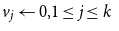$v_j\leftarrow 0, 1\le j\le k$ . We have the following telescoping property

\begin{align*} Z(G)&= x^{-1}(G,v_1\leftarrow 0)Z(G,\beta _1) \\[3pt] &= x^{-1}(G,v_1\leftarrow 0)x^{-1}(G,v_2\leftarrow 0, \beta _1)Z(G,\beta _2)\\[3pt] &= \prod _{1\le k\le m}x^{-1}(G,v_k\leftarrow 0, \beta _{k-1}), \end{align*}

under the convention that $\beta _0$ is an empty set of constraints. Suppose we algorithmically produce a sequence of estimations $y(G, v_k \leftarrow 0, \beta _{k-1}), 1\le k\le m$ of $x(G, v \leftarrow k, \beta _{k-1})$ up to multiplicative precision say $1/m^2$ . Namely,

\begin{align*} 1-1/m^2\le \frac {x(G, v_k \leftarrow 0, \beta _{k-1})}{y(G, v_k \leftarrow 0, \beta _{k-1})}\le 1+1/m^2. \end{align*}

Then $\hat Z(G) \triangleq \prod _k y^{-1}(G, v_k \leftarrow 0, \beta _{k-1})$ satisfies

\begin{align*} (1-1/m^2)^m=1-O(1/m)\le \frac {\hat Z(G)}{Z(G)} \le (1+1/m^2)^m =1+O(1/m), \end{align*}

and hence we achieve our goal of estimating $Z(G)$ up to multiplicative approximation better than any fixed constant $\epsilon$ for large $m$ . Thus our focus now is designing an algorithm for producing approximations $y(G, v \leftarrow n,\beta )$ of $x(G, v \leftarrow n, \beta )$ .

Our next step towards stating the Correlation Decay property is establishing a recursion structure exhibited by the marginal probabilities $x(G, v \leftarrow n, \beta )$ . This recursive structure in full generality was introduced in [Reference Gamarnik and Katz14] and we adopt it here as well.

We fix a graph $G=(V,E)$ , node $v\in V$ , and any set of constraints $\beta$ . Let $v_1,\ldots ,v_d$ be the neighbours of $v$ , where $d=d(v)$ is the degree of the node. For any sequence of integers $n_1,\ldots ,n_d\in [0,(1-\alpha )N]$ , we denote $(n_1,\ldots ,n_i)$ by $\bar n_i$ for short and consider the associated marginal probabilities

\begin{align*} x^i(\bar n_i)\triangleq x\left (G\setminus v, v_i\leftarrow n_i, \left(\beta , \left (v_j\leftarrow n_j, 1\le j\le i-1\right )\right )\right )\!. \end{align*}

Namely, this is the probability that when nodes $v_1,\ldots ,v_{i-1}$ are assigned values $n_1,\ldots ,n_{i-1}$ respectively (thus updating the set of constraints from $\beta$ to $\beta , v_j\leftarrow n_j, j\le i-1$ ), and $v$ is eliminated from $G$ , the node $v_i$ receives value $n_i$ . The vector $(x^i(\bar n_i), 1\le i\le d)$ of marginals is denoted by $\textbf {x}$ . For every $k$ , we let $S_k=[0,\min \left (N-k,(1-\alpha )N\right )]$ . Define the sequence $\left (f_n, n\in [0,(1-\alpha )N]\right )$ as follows:

(4) \begin{align} f_n({\textbf {x}}) = \frac {\sum \limits _{n_1, \ldots n_d \in S_n} x^1(\bar {n}_1) \ldots x^d(\bar {n}_d)} {\sum \limits _{m=0}^{(1-\alpha )N} \sum \limits _{n_1, \ldots n_d \in S_m} x^1(\bar {n}_1) \ldots x^d(\bar {n}_d)} . \end{align}

The recursive structure is stated in the following proposition which will be proved in the next section.

Proposition 2. The following relation holds for every $n\in [0,(1-\alpha )N]$ :

\begin{align*} x(G,v\leftarrow n, \beta )=f_n({\textbf {x}}). \end{align*}

Ultimately, we will use the recursion equation (4) to compute estimations $\textbf {y}$ of the true marginal probabilities $\textbf {x}$ recursively. We will introduce the notion of a Feasible Marginal Distribution for this problem setup in Section 3.1.2, and show that both the true marginals $\textbf {x}$ and the recursive estimates $\textbf {y}$ satisfy the definition. Our main Correlation Decay result states that provided two vectors $\textbf {x}$ and $\textbf {y}$ are Feasible Marginal Distributions and $\alpha \lt \alpha _\Delta$ , where $\alpha _\Delta$ satisfies equation (1), the following contraction property holds for every $n\in [0,(1-\alpha )N]$ and for some  $0\lt c=c(\alpha){\lt}{1}$ ,

\begin{align*} |f_n(\textbf {y})-f_n({\textbf {x}})|\le c \|\textbf {y}-{\textbf {x}}\|_\infty . \end{align*}

Namely, every iteration of the recursion encoded in $f_n$ decreases the estimation error geometrically. Provided the number of iterations is of the order $\Theta (\log m)$ , we will obtain the required upper $1/m^{\Omega (1)}$ on the estimation error. This is the Correlation Decay on the computation tree property which is the main technical underpinning of our work.

2.2 Integration

We now formally introduce the integration framework presented in the introduction, as well as the corresponding main theorem. Consider a hypergraph $G = (V,E)$ with $m$ vertices of some fixed maximum degree $\Delta$ (meaning each vertex in the hypergraph is a member of at most $\Delta$ edges). We will further assume that each vertex has at most $\eta$ neighbours, where a neighbour is defined as any other vertex which shares at least one edge (notice that $\eta \leq R \Delta$ ). We will define a hypergraph potential function to be any function $p({\textrm{n}}) \, : \, {\mathbb{R}}^{m} \rightarrow {\mathbb{R}}$ which takes the form

(5) \begin{align} p({\textrm{n}}) = \prod _{e \in E} \Phi _e({\textrm{n}}_e). \end{align}

We refer to each function $\Phi _e$ as the edge potential function for the edge $e$ . We wish to compute the expression

\begin{equation*}\int 1({\textrm{n}} \in [0,1]^{m}) p({\textrm{n}}) d\lambda ({\textrm{n}}),\end{equation*}

where $\lambda$ is the Lebesgue measure. Though we define the region of integration to be $[0,1]^m$ here for convenience, similar results will hold for any rectangular domain. Rather than computing a direct approximation of this integral, we will instead compute an approximation of the corresponding Riemann Sum. Fix some relaxation parameter $N$ , and let ${\mathcal{D}} = \{{\textrm{n}}/N| {\textrm{n}} \in {\mathbb Z}^m, 0 \leq n_v \lt N \ \forall v \in V\}$ . We define the partition function

(6) \begin{align} Z(G) = \sum \limits _{{\textrm{n}} \in {\mathcal{D}}} p({\textrm{n}}), \end{align}

which is equivalent to a traditional Riemann Sum scaled up by a factor of $N^m$ , with the goal of approximating this value. We will restrict ourselves to the setting where each $\Phi _e$ above satisfies

(7) \begin{align} c_e \leq \Phi _e({\textrm{n}}_e) \leq (1 - \delta )^{1/2\Delta } c_e\left (1 + \frac {\log (1 + \frac {1}{\eta })}{2\Delta }\right ), \end{align}

for some constant $c_e \gt 0$ unique to each edge and a universal constant $\delta \gt 0$ which controls the rate of convergence for our algorithm. In this setting, we will be able to show that the correlation decay property holds, once more allowing us to approximate the value $Z(G)$ . We will then be able to relate this approximation back to the value of the original integral. In particular, we will show the following.

Theorem 3 (Approximating integrals of hypergraph potential functions). Suppose we have a function $p$ taking the form of equation ( 5 ) with respect to some hypergraph $G$ . Further, suppose each function $\Phi _e$ is differentiable, satisfies the condition in equation ( 7 ), and there exists some $k \gt 0$ such that every $\Phi _e$ satisfies $\|\nabla \Phi _e({\textrm{n}}_e)\|_2 \leq k c_e$ for every ${\textrm{n}} \in [0,1]^m$ . Then, there exists an algorithm to produce an estimate $\tilde V$ of $\int 1({\textrm{n}} \in [0,1]^{m}) p({\textrm{n}}) d\lambda$ such that

\begin{equation*}\bigg | \frac {\tilde V}{\int 1({\textrm{n}} \in [0,1]^{m}) p({\textrm{n}}) d\lambda } - 1 \bigg | \leq O(1/m^2).\end{equation*}

Taking $k, \Delta ,$ and $ \eta$ to be constants, this algorithm will run in $m^{O(\log (m))}$ time.

In the course of our approximation algorithm, we will again need to iteratively restrict the domain of our partition function. Thus, we will introduce constraints of the form $v \leftarrow n$ , equivalent to restricting ${\textrm{n}}_v = n$ , and let $\beta$ be collections of such constraints. We then define ${\mathcal{D}}_\beta \subset {\mathcal{D}}$ to be the set of points in $\mathcal{D}$ that satisfy every constraint in $\beta$ . We will use the notation $(\beta , v \leftarrow n)$ to denote $\beta \cup \{v \leftarrow n\}$ . With this notation, we can define the following family of restricted partition functions

(8) \begin{align} Z(G, \beta ) = \sum \limits _{{\textrm{n}} \in {\mathcal{D}}_\beta } p({\textrm{n}}). \end{align}

We again use this to define a probability distribution over the assignments to each vertex in the hypergraph $G$ induced by the function $f$ and constraints $\beta$ . In particular, we define

\begin{equation*}x(G, v \leftarrow n, \beta ) = \frac {Z(G,(\beta , v \leftarrow n))}{Z(G,\beta )},\end{equation*}

which for each well formulated $\beta$ will define a probability distribution over the assignments 0 to $N-1$ for the vertex $v$ . Our algorithm will rely on computing an approximation $\tilde x(G, v \leftarrow n, \beta )$ of the above value, which will be done by exploiting the recursive nature of the problem. In particular, if we order the vertices 1 through $m$ and let $\beta _i = (v_j \leftarrow 0, j \leq i)$ for $i \in [0,m]$ , with $\beta _0 = \{\}$ , we can see

(9) \begin{align} Z(G) &= x^{-1}(G, v_1 \leftarrow 0, \beta _0 ) Z(G, \beta _1)\nonumber \\[3pt] &= \prod \limits _{i = 1}^{m} x^{-1}(G, v_i \leftarrow 0, \beta _{i-1}) Z(G, \beta _m)\nonumber \\[3pt] &= p(\textbf {0}) \prod \limits _{i = 1}^{m} x^{-1}(G, v_i \leftarrow 0, \beta _{i-1}), \end{align}

since $Z(G, \beta _m) = p(\textbf {0})$ by construction. Thus, if we can approximate the values of $x(G, v_i \leftarrow n, \beta _{i-1})$ within a factor of $\frac {1}{m^2}$ , we will be able to approximate $Z(G)$ within a factor of $\frac {1}{m}$ . We will accomplish this with the same high level technique used in the polytope section.

3.1 Preliminary results

This section will be primarily focused on providing a complete proof of Proposition 2. We will then provide a definition of a Feasible Marginal Distribution and establish a few related properties.

3.1.1 Proof of Proposition 2

We will now show how to write an expression for $x(G, v \leftarrow n, \beta )$ in terms of the variables $x^i(\bar {n}_i)$ , which represent the probability distribution over the assignments of adjacent vertices in smaller graphs. We will again assume that the vertex $v$ has $d \leq \Delta$ neighbours $v_1, \ldots v_d$ . We start this process by proving the next two Lemmas.

Lemma 4 (Recursive deconstruction).

\begin{align*} x(G, v \leftarrow n, \beta ) = \,& x(G, v \leftarrow 0, \beta ) \sum \limits _{n_1, \ldots n_d \in S_n} x^1(\bar {n}_1) \ldots x^d(\bar {n}_d) \end{align*}

Proof. Notice that

\begin{equation*}Z(G, (\beta , v \leftarrow 0)) = Z(G \setminus v, \beta ),\end{equation*}

and more generally

\begin{equation*}Z(G, (\beta , v \leftarrow n)) = \sum \limits _{(n_1, \ldots n_d) \in S_n^d} Z(G \setminus v, (\beta , (v_i \leftarrow n_i \forall i))).\end{equation*}

Using this, we have

\begin{align*} &x(G, v \leftarrow n, \beta )\\[3pt] &\quad = \frac {Z(G, (\beta , v \leftarrow n))}{Z(G,\beta )}\\[3pt] &\quad = \frac {Z(G, (\beta , v \leftarrow 0)) Z(G, (\beta , v \leftarrow n))}{Z(G, \beta ) Z(G \setminus v, \beta )}\\[3pt] &\quad =\frac {x(G, v \leftarrow 0, \beta )}{Z(G \setminus v, \beta )} Z(G, (\beta , v \leftarrow n))\\[3pt] &\quad = \frac {x(G, v \leftarrow 0, \beta )}{Z(G \setminus v, \beta )} \sum \limits _{(n_1, \ldots n_d) \in S_n^d} Z(G \setminus v, (\beta , (v_i \leftarrow n_i \forall i)))\\[3pt] &\quad = \frac {x(G, v \leftarrow 0, \beta )}{Z(G \setminus v, \beta )} \sum \limits _{n_1 \in S_n} Z(G\setminus v, (\beta , v_1 \leftarrow n_1)) \sum \limits _{(n_2, \ldots n_d) \in S_n^{d-1}} \frac {Z(G \setminus v, (\beta , (v_i \leftarrow n_i \forall i)))}{Z(G\setminus v, (\beta , v_1 \leftarrow n_1))}\\[3pt] &\quad = x(G, v \leftarrow 0, \beta ) \sum \limits _{n_1 \in S_n} \frac {Z(G\setminus v, (\beta , v_1 \leftarrow n_1))}{Z(G \setminus v, \beta )} \sum \limits _{(n_2, \ldots n_d) \in S_n^{d-1}} \frac {Z(G \setminus v, (\beta , (v_i \leftarrow n_i \forall i)))}{Z(G\setminus v, (\beta , v_1 \leftarrow n_1))}\\[3pt] &\quad = x(G, v \leftarrow 0, \beta ) \sum \limits _{n_1 \in S_n} x(G\setminus v, v_1 \leftarrow n_1, \beta ) \sum \limits _{(n_2, \ldots n_d) \in S_n^{d-1}} \frac {Z(G \setminus v, (\beta , (v_i \leftarrow n_i \forall i)))}{Z(G\setminus v, (\beta , v_1 \leftarrow n_1))}\\[3pt] &\quad = x(G, v \leftarrow 0, \beta ) \sum \limits _{n_1 \in S_n} x^1(\bar {n}_1) \sum \limits _{(n_2, \ldots n_d) \in S_n^{d-1}} \frac {Z(G \setminus v, (\beta , (v_i \leftarrow n_i \forall i)))}{Z(G\setminus v, (\beta , v_1 \leftarrow n_1))}\\[3pt] &\quad = x(G, v \leftarrow 0, \beta ) \sum \limits _{n_1 \in S_n} x^1(\bar {n}_1) \ldots \sum \limits _{n_d \in S_n} x^d(\bar {n}_d) \\[3pt] &\quad = x(G, v \leftarrow 0, \beta ) \sum \limits _{n_1 , \ldots n_d\in S_n} x^1(\bar {n}_1) \ldots x^d(\bar {n}_d), \end{align*}

where the second to last line is derived by repeating the same logic for each neighbour $v_i$ with a, appropriately modified value of $\beta$ .

Lemma 5 (Normalizing term).

\begin{align*} x(G, v \leftarrow 0, \beta ) = \frac {1}{\sum \limits _{m=0}^{(1-\alpha )N} \sum \limits _{n_1 , \ldots n_d\in S_m} x^1(\bar {n}_1) \ldots x^d(\bar {n}_d)}. \end{align*}

Proof. By construction, $\sum \nolimits _{m=0}^{(1-\alpha )N} x(G, v \leftarrow m, \beta ) = 1$ , since $((x(G, v\leftarrow m, \beta ))$ is a probability vector for $m \in [0,(1-\alpha )N]$ . Thus, by Lemma 4,

\begin{align*} 1 = \sum \limits _{m=0}^{(1-\alpha )N} x(G, v \leftarrow m, \beta ) = x(G, v \leftarrow 0, \beta ) \sum \limits _{m=0}^{(1-\alpha )N} \sum \limits _{n_1 , \ldots n_d\in S_m} x^1(\bar {n}_1) \ldots x^d(\bar {n}_d). \end{align*}

Rearranging terms, we have

\begin{equation*}x(G, v \leftarrow 0, \beta ) = \frac {1}{ \sum \limits _{m=0}^{(1-\alpha )N} \sum \limits _{n_1 , \ldots n_d\in S_m} x^1(\bar {n}_1) \ldots x^d(\bar {n}_d)}.\end{equation*}

Combining Lemmas 4 and 5, we immediately obtain Proposition 2.

3.1.2 Bounds on marginal probabilities

Section 3.2 will be dedicated to establishing a bound on the 1-norm of the function $f_n$ from equation (4). The bound we compute will need to hold not just on the true probability distribution $\textbf {x}$ , but also on any linear interpolation between the true distribution and our probability estimates. To do this, we identify the primary properties we need for the contraction to hold. Thus, we introduce the following notion of a Feasible Marginal Distribution, and show that our bound will hold on all such distributions.

Definition 1 (Feasible marginal distribution). Fix some $\textbf {w} = \{w_k \gt 0, 0 \leq k \leq (1- \alpha ) N\}$ . We say that $\textbf {w}$ is a Feasible Probability Distribution if

(10) \begin{align} \sum \limits _{k = 0}^{(1-\alpha )N} w_k &= 1, \\[-10pt] \nonumber \end{align}

(11) \begin{align} w_k &\geq w_{k+1}, \\[-10pt] \nonumber \end{align}

(12) \begin{align} w_{k} &= w_{k'} \quad \quad \forall k,k' \leq \alpha N. \\[10pt] \nonumber\end{align}

Further, we say $\textbf {y} = \{y^{\,j}(\bar {n}_j)| j \in \{1, \ldots d\}, \bar {n}_j \in [0,(1-\alpha )N]^j\}$ is a Feasible Marginal Distribution if for every $j \in \{1, \ldots d\}$ and $\bar {n}_{j-1} \in [0, (1-\alpha )N]^{j-1}$ where $(\beta , v_i \leftarrow n_i, i \lt j)$ forms a feasible set of constraints, the values $y_i = y^{\,j}(\bar {n}_{j-1}, i)$ for $i \in [0, (1-\alpha )N]$ form a Feasible Probability Distribution and for every $\bar {n}_j, \bar {m}_j \in [0, \alpha N]$ ,

(13) \begin{align} y^{\,j}(\bar {n}_j) = y^{\,j}(\bar {m}_j). \end{align}

We now show that $\textbf {x}$ as defined above is a Feasible Marginal Distribution. Firstly, observe from the problem’s construction that for any fixed $j, n_1, \ldots n_{j-1}$ , the set $\{x^j(\bar {n}_{j-1}, n_j)| n_j \in [0,(1-\alpha )N] \}$ forms a probability distribution when $(\beta , v_i \leftarrow n_i, i \lt j)$ forms a feasible set of constraints, meaning equation (10) is satisfied. Next, notice that $Z(G, (\beta , v \leftarrow n)) \geq Z(G, (\beta , v \leftarrow n+1))$ , since for every relaxed independent set where $v$ is assigned $n+1$ there is a relaxed in dependent that is identical except $v$ is assigned $n$ . Thus, we have that for every fixed $\bar {n}_{j-1}$ , $x^j(\bar {n}_{j-1},n_j) \geq x^j(\bar {n}_{j-1},n_j + 1)$ , so $\textbf {x}$ satisfies equation (11). Finally, we have that $Z(G, (\beta , v \leftarrow n)) = Z(G, (\beta , v \leftarrow n'))$ for every $0 \leq n,n' \leq \alpha N$ , since assigning any vertex a value in $[0, \alpha N]$ cannot violate any constraints. More generally, if every constraint in $\beta$ and $\beta '$ assigns a value of at most $\alpha N$ , then $Z(G, \beta ) = Z(G, \beta ')$ . This implies $\textbf {x}$ must satisfy equations (12) and (13). Therefore, $\textbf {x}$ is a Feasible Marginal Distribution.

Lemma 6 (Closure of feasible marginal distributions under $f_n$ ). Let ${\textrm{y}}$ be a Feasible Marginal Distribution, and let $y_n' = f_n({\textrm{y}})$ for $n \in [0, (1-\alpha )N]$ . Then, the set of $y_n'$ form a Feasible Probability Distribution.

Proof. Notice that $S_n = S_{n'}$ for any $n,n' \leq \alpha N$ by construction. By equation (4), we can clearly see this implies $f_n(\textbf {y}) = f_{n'}(\textbf {y})$ when $n,n' \leq \alpha N$ , so the values of $y_n'$ satisfy equation (12). Equation (10) is satisfied because

\begin{align*}\sum \limits _{n=0}^{(1-\alpha )N} f_n(\textbf {y}) = \frac {\sum \limits _{n=0}^{(1-\alpha )N} \sum \limits _{n_1, \ldots n_d \in S_n} y^1(\bar {n}_1) \ldots y^d(\bar {n}_d)} {\sum \limits _{m=0}^{(1-\alpha )N} \sum \limits _{n_1, \ldots n_d \in S_m} y^1(\bar {n}_1) \ldots y^d(\bar {n}_d)} = 1. \end{align*}

Finally, equation (11) is clearly satisfied because $S_n$ is non-increasing in $n$ and each term in the numerator sum is non-negative.

Lemma 7 (Linear interpolations of feasible Marginal distributions). Let ${\textrm{y}}$ and ${\textrm{z}}$ be two Feasible Marginal Distributions. Then, for any $w \in [0,1]$ , $w {\textrm{y}} + (1 - w) {\textrm{z}}$ is a Feasible Marginal Distribution, where the sum is taken pointwise.

The proof of Lemma 7 follows directly from the linearity of the four equations (10), (11), (12), and (13). These results will allow us to construct the contraction in sufficient generality. We conclude by proving two Lemmas about Feasible Probability Distributions.

Lemma 8. For any Feasible Probability Distribution ${\textrm{y}}$ , we have

\begin{equation*}y_i \leq \frac {1}{\alpha N}.\end{equation*}

Proof. By equation (12), for any $i,j \in [0, \alpha N]$ , the value of $y_i = y_j$ . There are $\alpha N$ such values, so each one must be no greater than $\frac {1}{\alpha N}$ . Additionally, for any $i$ , $y_i \leq y_0 \leq \frac {1}{\alpha N}$ by equation (11), finishing the proof.

Lemma 9. For any Feasible Probability Distribution $\textbf {y}$ , we have

\begin{equation*} \frac {\alpha }{1-\alpha } \le \sum _{i=0}^{\alpha N} y_i \le 1. \end{equation*}

Proof. The upper bound holds directly from equation (10). To prove the lower bound, first observe equation (10) implies 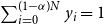$\sum \nolimits _{i = 0}^{(1-\alpha )N} y_i = 1$ . If 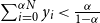$\sum \nolimits _{i = 0}^{\alpha N} y_i \lt \frac {\alpha }{1 - \alpha }$ , then it would have to be the case that $\sum \nolimits _{i = \alpha N + 1}^{(1 - \alpha ) N} y_i \gt \frac {1 - 2\alpha }{1-\alpha }$ . This would imply the last $1 -2\alpha$ terms in the sequence had a larger average value than the first $\alpha$ terms. Equation (11) implies this sequence must be decreasing, which is a contradiction. Thus, the bound must hold.

3.2 Proof of the polytope correlation decay property

In this section, we establish the key correlation decay property necessary to design the approximation algorithm. The primary result, occurring at the end of the section, will be a bound on $\|f_n(\textbf {y})\|_1$ defined in equation (4) with respect to a vertex $v$ with $d$ neighbours for any Feasible Marginal Distribution $\textbf {y}$ . The bound will be in terms of $\alpha$ and $d$ , and will be bounded away from 1 as $\alpha$ approaches $1/2$ for any fixed $d$ .

3.2.1 Expressions for partial derivatives

We now introduce the following two expressions to represent the numerator and denominator of equation (4):

\begin{align*} U_n &= \sum \limits _{n_1, \ldots n_d \in S_n} y^1(\bar {n}_1) \ldots y^d(\bar {n}_d),\\[3pt] L &= \sum \limits _{m=0}^{(1-\alpha )N} \sum \limits _{n_1, \ldots n_d \in S_m} y^1(\bar {n}_1) \ldots y^d(\bar {n}_d) = \sum \limits _{m=0}^{(1-\alpha )N} U_m. \\[-30pt] \end{align*}

In particular, we have that $f_n(\textbf {y}) = \frac {U_n}{L}$ . By the chain rule, we can see

(14) \begin{align} \frac {\partial f_n(\textbf {y})}{\partial y^{\,j}(\bar {n}_j)} = \frac {L \frac {\partial U_n(\textbf {x})}{\partial x^{j}(\bar {n}_{j})} - U_n \frac {\partial L(\textbf {x})}{\partial x^{j}(\bar {n}_{j})}}{L^2} . \end{align}

Let

\begin{align*} B_j(\bar {n}_{j-1}) &= y^1(\bar {n}_1) \ldots y^{j-1}(\bar {n}_{j-1}),\\[3pt] A_j(n, \bar {n}_j) &= \sum \limits _{n_{j+1}, \ldots n_d \in S_n} y^{j+1}(\bar {n}_{j+1}) \ldots y^{d}(\bar {n}_{d}). \end{align*}

Thus, for any $j \in [1,d]$ , we have

(15) \begin{align} U_n &= \sum \limits _{n_1, \ldots n_{j-1} \in S_n} B_j(\bar {n}_{j-1}) \sum \limits _{n_j \in S_n} y^{\,j}(\bar {n}_j) A_j(n,\bar {n}_j) , \\[-10pt] \nonumber \end{align}

(16) \begin{align} L &= \sum \limits _{m=0}^{(1-\alpha )N} \sum \limits _{n_1, \ldots n_{j-1} \in S_m} B_j(\bar {n}_{j-1}) \sum \limits _{n_j \in S_m } y^{\,j}(\bar {n}_j) A_j(m,\bar {n}_j) . \\[10pt] \nonumber \end{align}

Fix $j \in [1,d]$ and some $\bar {n}_j \in [0, (1-\alpha )N]^j$ . Letting $I(A)$ be the indicator variable for the event $A$ , we obtain

(17) \begin{align} \frac {\partial U_n}{\partial x^j(\bar {n}_j)} &= I(\bar {n}_j \in S_n^d) B_j(\bar {n}_{j-1}) A_j(n, \bar {n}_j), \\[-10pt] \nonumber \end{align}

(18) \begin{align} \frac {\partial L}{\partial x^j(\bar {n}_j)} &= \sum \limits _{m=0}^{(1-\alpha )N} I(\bar {n}_j \in S_m^d) B_j(\bar {n}_{j-1}) A_j(m, \bar {n}_j). \\[10pt] \nonumber \end{align}

Lemma 10. For any $j \in [1,d]$ , $n \in [0,(1-\alpha )N]$ , and $n_1, \ldots n_{j} \in [0,(1-\alpha )N]$ , we have

\begin{align*} A_j(n, \bar {n}_{j}) &\leq 1,\\[3pt] B_j(\bar {n}_{j-1}) &\leq \frac {1}{(\alpha N)^{j-1}}. \end{align*}

Proof. Recall that for any $\bar {n}_{d-1}$ , $y^d(\bar {n}_d)$ is a probability distribution as $n_d$ varies. Thus,

\begin{equation*}\sum \limits _{n_d \in S_n} y^d(\bar {n}_d) \leq \sum \limits _{n_d=0}^{(1-\alpha )N} y^d(\bar {n}_d) = 1.\end{equation*}

Iterating this process for vertices $v_d, v_{d-1}, \ldots v_{j+1}$ leads to the bound on $A_j$ . The bound on $B_j$ follows from Lemma 8.

Lemma 11. For any $j \in [1,d]$ , $n \in [0,(1-\alpha )N]$ , $n_1, \ldots n_{j} \in [0,\alpha N]$ , and $m_1, \ldots m_{j} \in [0,\alpha N]$ we have that

\begin{align*} A_j(n, \bar {n}_j) &= A_j(n, \bar {m}_j)\\[3pt] B_j(\bar {n}_{j-1}) &= B_j(\bar {m}_{j-1}) \end{align*}

Proof. By definition, we have 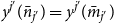$y^{j'}(\bar {n}_{j'}) = y^{j'}(\bar {m}_{j'})$ for any $j' \le j$ . Repeatedly substituting these equalities into the definitions of $A_j$ and $B_j$ produces the desired result.

We now move to bounding our numerator and denominator functions, $U_n$ and $L$ , directly.

Lemma 12 (Gradient denominator).

\begin{align*} L \geq \alpha N \end{align*}

Proof. Fix any $m \leq \alpha N$ . We will have that $S_m = [0, \min (N-m, (1-\alpha )N] = [0,(1-\alpha )N]$ . For any $n_1, \ldots n_{j-1}$ , $\sum \limits _{n_j = 0}^{\alpha N} y^{\,j}(\bar {n}_j) = 1$ since $\textbf {y}$ is a Feasible Marginal Distribution. Thus,

\begin{align*} \sum \limits _{n_1, \ldots n_d \in S_m} y^1(\bar {n}_1) \ldots y^d(\bar {n}_d) = \sum \limits _{n_1, \ldots n_d=0}^{(1-\alpha )N} y^1(\bar {n}_1) \ldots y^d(\bar {n}_d) = 1. \end{align*}

We then obtain

\begin{align*} L = \sum \limits _{m=0}^{(1-\alpha )N} \sum \limits _{n_1, \ldots n_d \in S_m} y^1(\bar {n}_1) \ldots y^d(\bar {n}_d) \geq \sum \limits _{m=0}^{\alpha N} \sum \limits _{n_1, \ldots n_d \in S_m} y^1(\bar {n}_1) \ldots y^d(\bar {n}_d) = \sum \limits _{m=0}^{\alpha N} 1 = \alpha N. \end{align*}

Lemma 13 (Upper bounds). For any $j \in [1,d]$ , $n \in [0,(1-\alpha )N]$ , and $n_1, \ldots n_{j-1} \in [0,(1-\alpha )N]$ , we have

\begin{align*} U_n &\leq 1, \\[3pt] L &\leq (1-\alpha )N, \\[3pt] \frac {\partial U_n(\textbf {x})}{\partial x^{j}(\bar {n}_{j})} &\leq \frac {1}{(\alpha N)^{j-1}}, \\[3pt] \frac {\partial L(\textbf {x})}{\partial x^{j}(\bar {n}_{j})} &\leq \frac {(1-\alpha )N}{(\alpha N)^{j-1}}. \end{align*}

Proof. We will show the bounds on $U_n$ and $\frac {\partial U_n(\textbf {x})}{\partial x^{j}(\bar {n}_{j})}$ . These will immediately imply the bounds on $L$ and $\frac {\partial L(\textbf {x})}{\partial x^{j}(\bar {n}_{j})}$ by definition. Writing $U_n$ in terms of $A_1$ in equation (15), we see that

\begin{align*} U_n = \sum \limits _{n_1 \in S_n} y^{\,j}(\bar {n}_1) A_1(n, \bar {n}_1) \leq \sum \limits _{n_1 \in S_n} y^{\,j}(\bar {n}_1) \leq 1, \end{align*}

where the first inequality follows from Lemma 10 and the second follows from equation (10). Similarly, we can write $\frac {\partial U_n(\textbf {x})}{\partial x^{j}(\bar {n}_{j})}$ in terms of $A_j$ and $B_j$ as in equation (17) to see that

\begin{equation*}\frac {\partial U_n(\textbf {x})}{\partial x^{j}(\bar {n}_{j})} = I(\bar {n}_j \in S_n^d) B_j(\bar {n}_{j-1}) A_j(n, \bar {n}_j) \leq B_j(\bar {n}_{j-1}) A_j(n, \bar {n}_j) \leq \frac {1}{(\alpha N)^j},\end{equation*}

where the last inequality follows from Lemma 10.

3.2.2 Upper bounds on partial derivatives

We are now obtain bounds on the value of the partial derivatives of $f(\textbf {y})$ , in order to ultimately bound $\|\nabla f(\textbf {y})\|_1$ . We will do this by using two different bounds on $\frac {\partial f(\textbf {y})}{\partial y^{\,j}(\bar {n}_j)}$ , depending on the value of $\bar {n}_j$ . We present the looser bound first, which applies to all partial derivatives.

Theorem 14 (Loose partial bound). For any $j \in [1,d]$ and $\bar {n}_j \in [0,(1-\alpha )N]^j$ ,

\begin{equation*}\left | \frac {\partial f({\textrm{y}})}{\partial y^{\,j}(\bar {n}_j)} \right | \leq \frac {(1-\alpha ) N}{(\alpha N)^{j+1}}\end{equation*}

Proof. As we saw in equation (14), we have

\begin{align*} \left |\frac {\partial f(\textbf {y})}{\partial y^{\,j}(\bar {n}_j)} \right | &= \left |\frac {L \frac {\partial U_n(\textbf {x})}{\partial x^{j}(\bar {n}_{j})} - U_n \frac {\partial L(\textbf {x})}{\partial x^{j}(\bar {n}_{j})}}{L^2} \right |\\[3pt] &\leq \frac {\max (L \frac {\partial U_n(\textbf {x})}{\partial x^{j}(\bar {n}_{j})}, U_n \frac {\partial L(\textbf {x})}{\partial x^{j}(\bar {n}_{j})}}{L^2}\\[3pt] & {\stackrel {\mbox{a}} \leq \, } \frac {\max (L \frac {\partial U_n(\textbf {x})}{\partial x^{j}(\bar {n}_{j})}, U_n \frac {\partial L(\textbf {x})}{\partial x^{j}(\bar {n}_{j})})}{(\alpha N)^2}\\[3pt] & {\stackrel {\mbox{b}} \leq \, } \frac {(1-\alpha ) N}{(\alpha N)^{j+1}}, \end{align*}

where inequality a follows from Lemma 12 and inequality b follows from Lemma 13.

As we will see in the next section, this bound alone will not be sufficiently tight. Next, we introduce a tighter bound on the partial derivative for cases where $\bar {n}_j \in [0,\alpha N]^j$ .

Theorem 15 (Tighter partial bound). For any $j \in [1,d]$ and $\bar {n}_j \in [0,\alpha N]^j$ ,

\begin{equation*}\left |\frac {\partial f({\textrm{y}})}{\partial y_j(\bar {n}_j)} \right | \leq \frac {j(1-2\alpha )(1-\alpha )^j}{\alpha ^{2j+1} N^{j}}.\end{equation*}

Proof.

\begin{align*} &\left |\frac {\partial f(\textbf {y})}{\partial y_j(\bar {n}_j)} \right |\\[3pt] &\quad= \frac {|L \frac {\partial U_n(\textbf {x})}{\partial x^{j}(\bar {n}_{j})} - U_n \frac {\partial L(\textbf {x})}{\partial x^{j}(\bar {n}_{j})}|}{L^2}\\[3pt] &\quad {\stackrel {\mbox{a}}\leq \,} \frac {1}{(\alpha N)^2} |L \frac {\partial U_n(\textbf {x})}{\partial x^{j}(\bar {n}_{j})} - U_n \frac {\partial L(\textbf {x})}{\partial x^{j}(\bar {n}_{j})}|\\[3pt] &\quad {\stackrel {{\mbox{b}}}= \,} \frac {1}{(\alpha N)^2} \left |\sum \limits _{m=0}^{(1-\alpha )N}\left [ \sum \limits _{\bar {m}_j \in S_m^j} \frac {\partial U_n(\textbf {x})}{\partial x^{j}(\bar {n}_{j})} B_j(\bar {m}_{j-1})y^{\,j}(\bar {m}_j) A_j(m, \bar {m}_j) - U_n I(\bar {n}_j \in S_m^j) B_j(\bar {n}_{j-1}) A_j(m, \bar {n}_j) \right ] \right | \\[3pt] &\quad {\stackrel {{\mbox{c}}}= \, } \frac {1}{(\alpha N)^2} \Bigg |\sum \limits _{m=0}^{(1-\alpha )N}\Bigg [ \sum \limits _{\bar {m}_j \in S_m^j} I(\bar {n}_j \in S_n^j) B_j(\bar {n}_{j-1}) A_j(n, \bar {n}_j) B_j(\bar {m}_{j-1})y^{\,j}(\bar {m}_j) A_j(m, \bar {m}_j) \\[3pt] &\qquad - \sum \limits _{\bar {p}_j \in S_n^j} B_j(\bar {p}_{j-1}) y^{\,j}(\bar {p}_j) A_j(n, \bar {p}_j) I(\bar {n}_j \in S_m^j) B_j(\bar {n}_{j-1}) A_j(m, \bar {n}_j) \Bigg ] \Bigg | \\[-3pt] &\quad {\stackrel {{\mbox{d}}}=\,} \frac {B_j(\bar {n}_{j-1})}{(\alpha N)^2} \Bigg |\sum \limits _{m=0}^{(1-\alpha )N}\Bigg [ \sum \limits _{\bar {m}_j \in S_m^j} \bigg \{ A_j(n, \bar {n}_j) B_j(\bar {m}_{j-1})y^{\,j}(\bar {m}_j) A_j(m, \bar {m}_j) \bigg \} \\[3pt] &\qquad - \sum \limits _{\bar {p}_j \in S_n^j} \bigg ( B_j(\bar {p}_{j-1}) y^{\,j}(\bar {p}_j) A_j(n, \bar {p}_j) A_j(m, \bar {n}_j) \bigg ) \Bigg ] \Bigg | \\[-20pt] \end{align*}

where inequality a comes from Lemma 12 , and equalities b and c come from applying equations (16), (18), (15), and (17). Equality d comes from factoring out $B_j(\bar {n}_{j-1})$ and observing that $\bar {n}_j \in S_n^j, S_m^j$ because we assumed it was in $[0,\alpha N]^j$ , which is a subset of $S_k$ for every $k$ .

We observe that when $\bar {m}_j, \bar {p}_j \in [0,\alpha N]^j$ , the expression above in the braces $\{\}$ will be equal to the expression in the parentheses $()$ by Lemma 11 and equation (13). Additionally, we bound the expression in the braces $\{\}$ . Using Lemmas 8 and 10, we have that for any $\bar {m}_j$

\begin{equation*}A_j(n, \bar {n}_j) B_j(\bar {m}_{j-1})y^{\,j}(\bar {m}_j) A_j(m, \bar {m}_j) \leq \frac {1}{(\alpha N)^j},\end{equation*}

with the same bound being true for the expression in the parentheses $()$ . Thus, we see

\begin{align*} \left |\frac {\partial f(\textbf {y})}{\partial y_j(\bar {n}_j)} \right | \leq & \frac {B_j(\bar {n}_{j-1})}{(\alpha N)^2} \sum \limits _{m=0}^{(1-\alpha )N}\Bigg [ \max \Bigg ( \sum \limits _{\bar {m}_j \in S_m^j, \bar {m}_j \not \in [0,\alpha N]^j} A_j(n, \bar {n}_j) B_j(\bar {m}_{j-1})y^{\,j}(\bar {m}_j) A_j(m, \bar {m}_j), \\[3pt] &\quad \sum \limits _{\bar {p}_j \in S_n^j, \bar {p}_j \not \in [0,\alpha N]^j} B_j(\bar {p}_{j-1}) y^{\,j}(\bar {p}_j) A_j(n, \bar {p}_j) A_j(m, \bar {n}_j) \Bigg ) \Bigg ] \\[3pt] {\stackrel {\mbox{a}}\leq \,}& \frac {B_j(\bar {n}_{j-1})}{(\alpha N)^2} \sum \limits _{m=0}^{(1-\alpha )N} \frac {N^j[(1-\alpha )^j - \alpha ^j]}{(\alpha N)^j} \\[3pt] {\stackrel {\mbox{b}}\leq \,}& \frac {1}{(\alpha N)^{j+1}} \sum \limits _{m=0}^{(1-\alpha )N} \frac {N^j[(1-\alpha )^j - \alpha ^j]}{(\alpha N)^j} \\[3pt] =\, & \frac {(1-\alpha )N}{(\alpha N)^{j+1}} \left (\frac {(1-\alpha )^j}{\alpha ^j} - 1 \right ) \end{align*}

Inequality b comes from Lemma 10. Inequality a comes from the bound above, and observing that there are at most $N^j(1-\alpha )^j$ vectors in $S_m^j$ or $S_n^j$ and exactly $N^j \alpha ^j$ vectors in $[0,\alpha N]^j$ .

3.2.3 Bounding the gradient

We are now able to prove a bound on the gradient of the function in equation (4) in terms of $d$ and $\alpha$ .

Theorem 16 (Bounded gradient). For any $n \in [0, (1-\alpha )N]$ ,

\begin{equation*}\|\nabla f_n({\textrm{y}})\|_1 \leq \frac {2d(1-\alpha )}{\alpha }\left (\frac {(1-\alpha )^d}{\alpha ^d} - 1 \right ).\end{equation*}

In particular, when $G$ has maximum degree $\Delta$ , $\|\nabla f_n(\textbf {y})\|_1 \lt 1$ so long as $\alpha \gt \alpha _\Delta$ , where $\alpha _\Delta$ is defined in equation ( 1 ).

Proof. First, fix some $j \in [1,d]$ . Notice that there are exactly $(\alpha N)^j$ different $\bar {n}_j \in [0,\alpha N]^j$ . Further, there are $(1-\alpha )^j N^j$ different $\bar {n}_j \in [0,(1-\alpha ) N]^j$ , meaning there are $N^j[(1-\alpha )^j - \alpha ^j]$ vectors in the latter not in the former.

Using theorems14 and 15, we obtain

\begin{align*} \sum \limits _{\bar {n}_j \in [0,(1-\alpha )N]^j} \left | \frac {\partial f(\textbf {y})}{\partial y^{\,j}(\bar {n}_j)} \right | &\leq (\alpha N)^j \frac {(1-\alpha )N}{(\alpha N)^{j+1}} \left (\frac {(1-\alpha )^j}{\alpha ^j} - 1 \right ) + N^j((1-\alpha )^j - \alpha ^j) \frac {(1-\alpha )N}{(\alpha N)^{j+1}}\\[3pt] &= \frac {2(1-\alpha )}{\alpha }\left (\frac {(1-\alpha )^j}{\alpha ^j} - 1 \right ). \end{align*}

Using this, we can conclude

\begin{align*} \|\nabla f_n(\textbf {y})\|_1 &= \sum \limits _{j=1}^d \sum \limits _{\bar {n}_j \in [0,(1-\alpha )N]^j} \left | \frac {\partial f(\textbf {y})}{\partial y^{\,j}(\bar {n}_j)} \right |\\[3pt] &\leq \sum \limits _{j=1}^d \frac {2(1-\alpha )}{\alpha }\bigg (\frac {(1-\alpha )^j}{\alpha ^j} - 1 \bigg )\\[3pt] &\leq \sum \limits _{j=1}^d \frac {2(1-\alpha )}{\alpha }\bigg (\frac {(1-\alpha )^d}{\alpha ^d} - 1 \bigg )\\[3pt] &= \frac {2d(1-\alpha )}{\alpha }\bigg (\frac {(1-\alpha )^d}{\alpha ^d} - 1 \bigg ). \\[-24pt] \end{align*}

Evaluated at $\Delta = 3$ , we obtain $\alpha _3 \approx 0.488$ . Take $\alpha = 0.5 - c/\Delta ^\gamma$ , with $c$ a constant not dependent on $\Delta$ and $\gamma \gt 0$ . When $\gamma \lt 2$ , we have

\begin{equation*}\lim _{\Delta \rightarrow \infty } \frac {2\Delta (0.5 + c/\Delta ^\gamma )}{(0.5 - c/\Delta )^\gamma }\left (\frac {(0.5 + c/\Delta ^\gamma )^\Delta }{(0.5 - c/\Delta ^\gamma )^\Delta } - 1 \right ) = \infty .\end{equation*}

But, when $\gamma = 2$ and $c \lt \frac {1}{8}$ , we have

\begin{equation*}\lim _{\Delta \rightarrow \infty } \frac {2\Delta (0.5 + c/\Delta ^2)}{(0.5 - c/\Delta )^2}\left (\frac {(0.5 + c/\Delta ^2)^\Delta }{(0.5 - c/\Delta ^2)^\Delta } - 1 \right ) = 8c \lt 1.\end{equation*}

Thus, $\alpha _\Delta$ is of the form $0.5 - O(1/\Delta ^2)$ .

3.3 A counting algorithm

In this section, we design an algorithm to approximate $Z(G)$ . We first demonstrate how to use the contraction proven in Section 3.2 to design a recursive algorithm which approximates $x(G, v \leftarrow n, \beta )$ with error decaying geometrically in the recursion depth. With this, we will present the approximation algorithm and formalize the argument from Section 2.

Algorithm 1

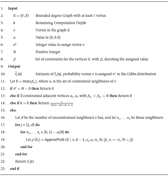
ApproxProb

Algorithm 1 Long description

An equation describing an algorithm to approximate the probability that a vertex v is assigned an integer value n* in a graph G. The algorithm involves checking constraints and computing probabilities based on the remaining computation depth k. It includes conditions for returning zero and calculating the probability based on unconstrained neighbors.

3.3.1 Approximating probabilities

In this section, we introduce Algorithm1, ApproxProb. This algorithm recursively computes an approximation $y(G, v \leftarrow n, \beta )$ of $x(G, v \leftarrow n, \beta )$ .

Lemma 17. Take some arbitrary graph $G$ with degree bounded by $\Delta$ , as well as some parameters $N, \alpha , \beta$ satisfying $\|\nabla f^v_n\|_1 = c \lt 1$ , where $f^v_n$ is the function from equation ( 4 ), for each vertex $v$ in every subgraph of $G$ with any $\beta$ for the particular values of $N$ and $\alpha$ . Pick any computation depth $k \gt 0$ . Algorithm 1 called with parameters $G, k, \alpha , N,$ and $ \beta$ will produce an approximation $y = y(G, v \leftarrow n^*, \beta )$ of $x = x(G, v \leftarrow n^*, \beta )$ satisfying

\begin{equation*}|y - x| \leq c^k.\end{equation*}

Further, it will do so in time $N^{O(k\Delta )}$ .

Proof. We will first need to establish that the estimated marginal probabilities $\textbf {y}$ computed on line 19 form a Feasible Marginal Distribution. We will do so inductively, starting with $k=1$ , as it is the first time we compute such a $\textbf {y}$ . When $k = 1$ , $\textbf {y}$ will form a Feasible Marginal Distribution by construction. The Feasible Probability Distribution requirements will be satisfied by the value returned on line 14, since it will be the uniform probability measure over all feasible values of $n^*$ . Further, for any $j \in \{1, \ldots d\}$ and $\bar {n}_{j}, \bar {m}_j \in [0,\alpha N]^j$ , $y^{\,j}(\bar {n}_j) = y^{\,j}(\bar {m}_j) = \frac {1}{(1-\alpha )N}$ , satisfying the final requirement.

Proceeding by induction for $k \gt 1$ , we have that the Feasible Probability Distribution requirements will be satisfied by Lemma 6 and the inductive hypothesis. Additionally, observe that if $n,m \leq \alpha N$ , changing $u \leftarrow n$ to $u \leftarrow m$ in a constraint set $\beta$ will not change the result of running ApproxProb. This is because $u$ assigned to either value cannot violate any constraints. Finally, notice that the vector $\textbf {y}$ computed in a call to ApproxProb does not depend on $n^*$ , and $f_n = f_m$ for any $n,m \le \alpha N$ . Thus, the vector $\textbf {y}$ computed on line 19 must satisfy equation (13), so $\textbf {y}$ is a Feasible Marginal Distribution.

We will now show the main result via induction. For the base case, suppose that $k=1$ . Let $\textbf {x}$ be the true values of the variables $x^i(\bar {n}_i)$ according to the Gibbs distribution of their corresponding graphs. Let $\textbf {y}$ be the values of the variables computed in the execution of the algorithm on line 19. By the mean value theorem, there must exists some $\textbf {z}$ , which is a linear interpolation of $\textbf {y}$ and $\textbf {x}$ such that

\begin{equation*}f_n^v({\textbf {x}}) - f_n^v(\textbf {y}) = \nabla f^v_n(\textbf {z}) \cdot ({\textbf {x}} -\textbf {y}).\end{equation*}

By Lemma 7, $\textbf {z}$ must also be a Feasible Marginal Distribution. Further, every entry in $\textbf {x}$ and $\textbf {y}$ is non-negative and bounded by 1. Thus,

\begin{equation*}|f_n^v({\textbf {x}}) - f_n^v(\textbf {y})| \leq \|\nabla f^v_n(\textbf {z})\|_1 \|{\textbf {x}} -\textbf {y}\|_\infty \leq c.\end{equation*}

We now induct over the values of $k$ . Once again, let $\textbf {x}$ be the true values of the variables $x^i(\bar {n}_i)$ , and let $\textbf {y}$ be the values computed on line 19 during the outermost layer of the recursion. Notice that any entries of $\textbf {y}$ which are 0 will also be 0 in $\textbf {x}$ . This, combined with the inductive hypothesis, implies that $\|{\textbf {x}} - \textbf {y}\|_\infty \leq c^{k-1}$ . Thus, using the same logic as above, we can use the mean value theorem to show that $|f^v_n({\textbf {x}}) - f^v_n(\textbf {y})\| \leq c^k$ as desired.

Additionally, we wish to analyse the runtime of Algorithm1. Let $T(k)$ denote the runtime of the algorithm with the input $k$ , and notice that $T(0) = O(1)$ . For runs with higher values of $k$ , the limiting time step will be computing the recursive calls on line 20. There will be at most $(1-\alpha )^\Delta N^\Delta$ iterations, and each will take $O(\Delta ^2)$ time to update the values of $\beta$ . Therefore, we get that $T(k) = O((1-\alpha )^\Delta N^\Delta \Delta ^2 T(k-1))$ implying that $T(k) = O\left (\left ((1-\alpha )^\Delta N^\Delta \Delta ^2\right )^k\right )$ . Since we are interested in the runtime in terms of $\Delta$ , $k$ and $N$ , this gets us that $T(k) = N^{O(k\Delta )}$ .

Algorithm 2

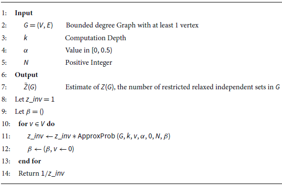
ApproxZ

Algorithm 2 Long description

The table outlines an algorithm named ApproxZ. It starts with input parameters including a bounded degree graph G, computation depth k, value alpha, and positive integer N. The output is an estimate of Z(G), the number of restricted relaxed independent sets in G. The algorithm initializes variables and iterates over each vertex in the graph, updating the estimate using a function ApproxProb. The final output is the reciprocal of the initialized variable z_inv.

3.3.2 Counting algorithm

We now introduce Algorithm2 ApproxZ, which will approximately compute $Z(G)$ , the number of restricted relaxed independent sets in the graph $G$ . This algorithm directly computes the telescoping definition of $Z(G)$ using the approximated marginal probabilities produced by Algorithm1. We will show the following main result.

Theorem 18. For any graph $G$ of maximum degree $\Delta$ with $m$ vertices, Algorithm 2 will produce an estimate $\hat Z(G)$ satisfying

\begin{equation*}1 - O(1/m) \leq \frac {\hat Z(G)}{Z(G)} \leq O(1/m),\end{equation*}

for any $N$ and any $\alpha \gt \alpha _\Delta$ for some $k$ which is $O(\log mN)$ . Further, the algorithm will run in $N^{O(\Delta \log Nm)}$ time.

Proof. Since $\alpha \gt \alpha _\Delta$ , we have that $\|\nabla f_n\|_1 \leq c \lt 1$ with respect to every vertex $v$ in ever subgraph of $G$ . Observe that equations (10) and (11) together imply that $y(G, v \leftarrow 0, \beta ) \geq \frac {1}{(1-\alpha ) N + 1}$ . Thus, letting $k = \log _c\left (\frac {1}{((1-\alpha )\alpha N + 1)m^2}\right )$ in the execution of Algorithm2, Lemma 17 says the estimates $y(G, v_k \leftarrow 0, \beta _{k-1})$ of $x(G, v_k \leftarrow 0, \beta _{k-1})$ will satisfy

\begin{equation*}|x(G, v_k \leftarrow 0, \beta _{k-1})-y(G, v_k \leftarrow 0, \beta _{k-1})| \leq \frac {1}{((1-\alpha ) N + 1)m^2} \leq \frac {y(G, v_k \leftarrow 0, \beta _{k-1})}{m^2}.\end{equation*}

Dividing both sides of the equation by $y(G, v_k \leftarrow 0, \beta _{k-1})$ results in

\begin{equation*} \left|\frac {x(G, v_k \leftarrow 0, \beta _{k-1})}{y(G, v_k \leftarrow 0, \beta _{k-1})} - 1 \right| \leq \frac {1}{m^2}.\end{equation*}

As discussed in Section 2, this bound is sufficient to show that the estimate $\hat Z(G)$ satisfies

\begin{equation*}1 - O(1/m) \leq \frac {\hat Z(G)}{Z(G)} \leq O(1/m).\end{equation*}

We finish by noting that since $c \lt 1$ , $k$ is $O(\log mN)$ for constant $\alpha$ . The bound on the running time follows directly from the bound in Lemma 17.

3.4 From counting to volumes

Now that we have an algorithm to count restricted relaxed independent sets, we move to showing how one can approximate the volume of $\mathcal{P}_{\textrm {IS}}(G, \alpha )$ using this discrete approximation.

Fix an arbitrary graph $G = (V,E)$ with $V = \{v_1, \ldots v_m\}$ , where each vertex has degree at most $\Delta$ . We define a set of graphs $G_n = (\{v_1, \ldots v_n\}, E_n)$ where $E_n = \{(v_i,v_j) \in E| i,j \leq n\}$ , so that $G_m = G$ . Additionally, fix $\alpha \geq \alpha _\Delta$ and $N$ . Since we will be inducting over the size of the graph, we will redefine $\beta$ to be a set of constraints of the form $x_i \leq c$ , and have $\beta _i$ denote the tightest constraint on $x_i$ . In particular, meaning any $\textbf {x}$ satisfying every constraint in $\beta$ satisfies $x_i \leq \beta _i$ . Similarly, we will redefine $v_i \leftarrow c$ to be the set of constraints $\{x_j \le N-c|(v_i, v_j) \in E\}$ . We assume that $\alpha N \leq \beta _i \leq (1-\alpha )N$ . Under this setup, we define the following family of polytopes,

\begin{equation*}{\mathbb Q}(G_n, \alpha , \beta ) = \{{\textbf {x}} \in {\mathbb{R}}^n: 0 \leq x_i \leq \beta _i\ \forall i\in [1,n], x_i + x_j \leq N \ \forall (v_i,v_j) \in E_n\}.\end{equation*}

We will show that for any such polytope, we can approximate its volume by counting the number of restricted relaxed independent sets in $G$ . To do this, we define the following two sets,

\begin{align*} {\mathcal{U}}(G_n, \alpha , \beta ) &= \{{\textbf {x}} \in {\mathbb Z}^n: 0 \leq x_i \leq \beta _i \ \forall i\in [1,n], x_i + x_j \leq N \ \forall (v_i,v_j) \in E_n\},\\[3pt] {\mathcal{L}}(G, \alpha , \beta ) &= \{{\textbf {x}} \in {\mathbb Z}^n: 0 \leq x_i \leq \beta _i - 1 \ \forall i\in [1,n], x_i + x_j \leq N-2 \ \forall (v_i,v_j) \in E_n\}. \end{align*}

Notice that $\frac {{\mathbb Q}(G, \alpha , \beta )}{N^m} \subseteq \mathcal{P}_{\textrm {IS}}(G, \alpha )$ , and when $\beta$ is such that $\beta _i = (1-\alpha )N, \forall i$ , $|{\mathcal{U}}(G, \alpha , \beta )| = Z(G)$ and $\frac {{\mathbb Q}(G, \alpha , \beta )}{N^m} = \mathcal{P}_{\textrm {IS}}(G, \alpha )$ .

Lemma 19 (Volume bound). For any graph $G$ and any $n, \beta , \alpha , N$ ,

\begin{align*}|{\mathcal{L}}(G, \alpha , \beta )| \leq \operatorname {Vol}({\mathbb Q}(G_n, \alpha , \beta )) \leq |{\mathcal{U}}(G_n, \alpha , \beta )|. \end{align*}

Now, we move on to the main theorem of this section.

Theorem 20 (Volume approximation). For any graph $G$ and any of $n, \beta , \alpha , N$ ,

\begin{align*} \left (1 - \frac {n}{\alpha N}\right ) |{\mathcal{U}}(G_n, \alpha , \beta )| \leq \operatorname {Vol}({\mathbb Q}(G_n, \alpha , \beta )) \leq |{\mathcal{U}}(G_n, \alpha , \beta )|. \\[-15pt] \end{align*}

Proof. Let ${\textbf {x}} \in {\mathcal{U}}(G_n, \alpha , \beta )$ be picked uniformly at random. Further, let $\mu _\beta ^n = {\mathbb{P}}({\textbf {x}} \not \in {\mathcal{L}}(G, \alpha , \beta )) = \frac {|{\mathcal{U}}(G_n, \alpha , \beta )| - |{\mathcal{L}}(G, \alpha , \beta )|}{|{\mathcal{U}}(G_n, \alpha , \beta )|}$ . We will show $\mu _\beta ^n \leq \frac {n}{\alpha N}$ by induction on $n$ . This will directly imply the result by Lemma 19 since $|{\mathcal{L}}(G_n, \alpha , \beta )| = (1 - \mu _\beta ^n) |{\mathcal{U}}(G_n, \alpha , \beta )|$ . In the base case, if $n = 1$ , then $\mu _\beta ^1 = {\mathbb{P}}(x_1 \leftarrow \beta _1) = \frac {1}{\beta _1+1} \leq \frac {1}{\alpha N}$ , since $x_1$ is uniformly distributed over $[0,\beta _1]$ and $\beta _1 \geq \alpha N$ .

We now proceed by induction. First, notice that for any ${\textbf {x}} \in {\mathcal{U}}(G_n, \alpha , \beta )$ , replacing the $n$ th entry of $\textbf {x}$ with any smaller value will produce a new ${\textbf {x}}' \in {\mathcal{U}}(G_n, \alpha , \beta )$ . In particular, this means for any $0 \leq j \leq i$ , it must be that ${\mathbb{P}}(x_n \leftarrow i) \leq {\mathbb{P}}(x_n \leftarrow j)$ . Thus,

\begin{equation*}{\mathbb{P}}(x_n \leftarrow i) \leq \frac {{\mathbb{P}}(x_n \leftarrow i)}{\sum _{j=0}^i{\mathbb{P}}(x_n \leftarrow j)} \leq \frac {{\mathbb{P}}(x_n \leftarrow i)}{(i+1){\mathbb{P}}(x_n \leftarrow i)} = \frac {1}{i+1},\end{equation*}

and since $\beta _n \geq \alpha N$ , we get that ${\mathbb{P}}(x_n \leftarrow \beta _i) \leq \frac {1}{\alpha N}$ .

Next, consider any ${\textbf {x}} \in {\mathcal{U}}(G_n, \alpha , \beta )$ with $x_n = k$ where ${\textbf {x}} \not \in {\mathcal{L}}(G, \alpha , \beta )$ . It must be that either $x_n = \beta _n$ or $(x_1, \ldots x_{n-1}) \not \in {\mathcal{L}}(G_{n-1}, \alpha , (\beta , v_n \leftarrow k))$ . Notice that $k \leq (1-\alpha )N$ , since $\beta _n \leq (1-\alpha )N$ by assumption. Therefore, we can use the inductive hypothesis to see

\begin{align*} \mu _\beta ^n &= {\mathbb{P}}(x_n \leftarrow \beta _n) + \sum \limits _{i=0}^{\beta _i-1} {\mathbb{P}}(x_n \leftarrow i) \mu ^{n-1}_{(\beta , x_n \leftarrow i)} \\[3pt] &\leq \frac {1}{\alpha N} + \sum \limits _{i=0}^{\beta _i-1} {\mathbb{P}}(x_n \leftarrow i) \frac {n-1}{\alpha N}\\[3pt] &\leq \frac {n}{\alpha N}. \end{align*}

With this analysis, we are ready to complete the proof of our main result, Theorem1.

Proof of Theorem 1. We will actually prove an asymptotically stronger result, namely that there is an algorithm running in $m^{O(\log m)}$ time which produces a value $\tilde V$ satisfying

\begin{equation*}1 - O(1/m) \le \frac {\tilde V}{\operatorname {Vol}(\mathcal{P}_{\textrm {IS}}(G,\alpha ))} \leq 1 + O(1/m)\end{equation*}

when $G$ is an $m$ node graph with a maximum degree of $\Delta$ and $\alpha \gt \alpha _\Delta$ . The proof which follows can be modified to a proof of the main theorem by setting $N$ to be $O(m/\epsilon )$ and modifying Theorem18 to have $k$ be $O(\log m/\epsilon )$ .

We start by setting $N = \frac {m^2}{\alpha }$ . Let $\beta$ be such that $\beta _i = (1-\alpha )N$ for every $i$ . We have that $\mathcal{P}_{\text{IS}}(G,\alpha ) = \frac {{\mathbb Q}(G, \alpha , \beta )}{N^m}$ . By Theorem20, we have

\begin{equation*}\left (1 - \frac {m}{\alpha N}\right )|{\mathcal{U}}(G, \alpha , \beta )| = \left (1 - \frac {1}{m}\right ) |{\mathcal{U}}(G, \alpha , \beta )| \leq \operatorname {Vol}({\mathbb Q}(G, \alpha , \beta )) \leq |{\mathcal{U}}(G, \alpha , \beta )|,\end{equation*}

as a result

\begin{align*} |{\mathcal{U}}(G, \alpha , \beta )| - \operatorname {Vol}({\mathbb Q}(G, \alpha , \beta ))| &= |{\mathcal{U}}(G, \alpha , \beta )| - \operatorname {Vol}({\mathbb Q}(G, \alpha , \beta ))\\[3pt] &\leq \frac {|{\mathcal{U}}(G, \alpha , \beta )|}{m}\\[3pt] &\leq \frac {2 \operatorname {Vol}({\mathbb Q}(G, \alpha , \beta ))}{m} , \end{align*}

where the last inequality follows from $1 - \frac {1}{m} \geq \frac {1}{2}$ (unless the graph is trivial) implying that $2\operatorname {Vol}({\mathbb Q}(G, \alpha , \beta )) \geq |{\mathcal{U}}(G, \alpha , \beta )|$ . Additionally, we have that $|{\mathcal{U}}(G, \alpha , \beta )| = Z(G)$ by construction. Theorem18 implies the existence of a deterministic algorithm to produce an estimate $\tilde {Z}(G)$ satisfying $|\tilde {Z}(G) - |{\mathcal{U}}(G, \alpha , \beta )|| \leq c|{\mathcal{U}}(G, \alpha , \beta )|/m$ for some universal constant $c$ . Thus, we get

\begin{align*} |\operatorname {Vol}({\mathbb Q}(G, \alpha , \beta )) - \tilde {Z}(G, \alpha )| &\leq |\operatorname {Vol}({\mathbb Q}(G, \alpha , \beta )) - |{\mathcal{U}}(G, \alpha , \beta )|| + ||{\mathcal{U}}(G, \alpha , \beta )| - \tilde {Z}(G,\alpha )|\\[3pt] &\leq \frac {2}{m} \operatorname {Vol}({\mathbb Q}(G, \alpha , \beta )) + \frac {c}{m} |{\mathcal{U}}(G, \alpha , \beta )|\\[3pt] &\leq \frac {2}{m} \operatorname {Vol}({\mathbb Q}(G, \alpha , \beta )) + \frac {2c}{m} \operatorname {Vol}({\mathbb Q}(G, \alpha , \beta ))\\[3pt] &= \frac {2c +2}{m} \operatorname {Vol}({\mathbb Q}(G, \alpha , \beta )), \end{align*}

where the last inequality again holds because $2\operatorname {Vol}({\mathbb Q}(G, \alpha , \beta )) \geq |{\mathcal{U}}(G, \alpha , \beta )|$ . Therefore, we can take $\tilde V = \frac {\tilde {Z}(G, \alpha )}{N^m}$ to be our estimate of the volume of $\mathcal{P}_{\text{IS}}$ to see

\begin{equation*}|\operatorname {Vol}(\mathcal{P}_{\text{IS}}) - \frac {\tilde {Z}(G, \alpha )}{N^m}| = \frac {|\operatorname {Vol}({\mathbb Q}(G, \alpha , \beta )) - \tilde {Z}(G, \alpha )|}{N^m} \leq \frac {2c+2}{mN^m } \operatorname {Vol}({\mathbb Q}(G, \alpha , \beta )) = \frac {2c+2}{m} \operatorname {Vol}(\mathcal{P}_{\text{IS}}). \end{equation*}

Additionally, substituting in the value of $N$ , the algorithm from Theorem18 will run in $m^{O(\Delta \log m)}$ time.

3.5 Barriers to the $\alpha = 0$ case

In this section, we discuss some challenges we encounter when designing an algorithm to compute the volume of the unrestricted ( $\alpha = 0$ ) independent set polytope. While the gradient bound given in Section 3.2 is loose and some adjustment to the argument may admit an asymptotic improvement on our values of $\alpha _\Delta$ , it clearly will not generalize to $\alpha = 0$ . In fact, we have been able to show computationally that the values of $|\nabla f_n|_1$ , with $f_n$ defined as in equation (4) exceeds 1 in bounded degree graphs when $\alpha = 0$ . We set $N = 64$ and take a 4-regular tree of depth 50, and assigned each leaf vertex 0 with probability 1. We were than able to repeatedly apply equation (4) to produce a probability distribution for the assignment of the vertices at each level of the tree. We know that correlation decay holds on trees [Reference Gamarnik and Ramanan16], so the probability distributions quickly converges to a fixed point distribution. At depth 50, the probability of a vertex being assigned a value $n$ had converged within 5 significant decimal places.

We evaluated $|\nabla f_n({\textbf {x}})|_1$ for each $n$ with this probability distribution $\textbf {x}$ . We found that for $n \leq 13$ , $|\nabla f_n({\textbf {x}})|_1 \gt 1$ . When we modified $N$ , we found that roughly the same proportion of values $n$ satisfied $|\nabla f_n({\textbf {x}})|_1 \gt 1$ . Increasing the degree of the tree increased the number of $n$ where $|\nabla f_n({\textbf {x}})|_1 \gt 1$ .

Since we initialized each leaf node with the same value, every vertex at a specified depth in our tree will have the same probability distribution over $[0,N]$ . Thus, we can modify equation (4) to be only a function of $x_0, \ldots x_N$ , where $x_i$ is the probability a vertex of depth one below our current vertex is assigned $i$ . This allows us to construct the $N+1 \times N+1$ matrix $M$ , where $M_{ij} = \frac {\partial f_i({\textbf {x}})}{\partial x_j}$ . In all of the cases above, we found that this matrix $M$ had a largest singular value greater than 1, and thus had an operator norm exceeding 1. This seems to suggest that methods of showing correlation decay which relies on showing a universal single step contraction, such as one similar to ([Reference Chen, Liu, Mani and Moitra10]) does not succeed. It is possible that methods based on multi-step contraction or based on other single step but non-spectral type of contraction do succeed. We leave it as a very interesting question for further research.

4.1 Preliminary results

Fix a vertex $v \in V$ and a set of constraints $\beta$ . Let $v_1, \ldots v_{\eta '}$ , $\eta ' \leq \eta$ , be the unconstrained neighbours of $v$ (we will take $v_0$ to be the vertex $v$ itself). For any sequence $n_1, \ldots n_{\eta '} \in [0,N-1]$ and any $i \in [1,\eta ']$ , we will use $\bar n_i$ to denote $(n_1, \ldots n_i)$ . For each such sequence, we can consider the associated marginal probabilities

\begin{equation*}x^i(\bar n_i) \triangleq x(G \setminus v, v_i \leftarrow n_i, (\beta , (v_j \leftarrow n_j, j \lt i))). \end{equation*}

We will use $\textbf {x}$ to denote the vector of marginals $(x^i(\bar n_i), 1 \leq i \leq \eta ', \bar n_i \in [0,N-1]^i)$ . Notice that for any fixed $i$ and $\bar n_{i-1}$ , we have

\begin{equation*}\sum \limits _{n_i=0}^{N-1} x^i(\bar n_i) = \frac {\sum \limits _{n_i=0}^{N-1} Z(G \setminus v, (\beta , (v_j \leftarrow n_j, j \leq i)))}{Z(G \setminus v, (\beta , (v_j \leftarrow n_j, j \lt i)))} =\frac {Z(G \setminus v, (\beta , (v_j \leftarrow n_j, j \lt i)))}{Z(G \setminus v, (\beta , (v_j \leftarrow n_j, j \lt i)))} = 1, \end{equation*}

which inductively implies

(19) \begin{align} \sum \limits _{n_1, \ldots n_i \in [0,N-1]} \prod \limits _{j=1}^i x^i(\bar n_i) = 1. \end{align}

We now define the function

(20) \begin{align} g_n({\textbf {x}}) = \frac {\sum \limits _{n_1, \ldots n_{\eta '} \in [0,N-1]} \prod \limits _{j=1}^{\eta '} x^j(\bar n_j) \prod \limits _{e \in E, v \in e} \Phi _{e}(n, {\textrm{n}}_{e\setminus v})} {\sum \limits _{n_0, n_1, \ldots n_{\eta '} \in [0,N-1]} \prod \limits _{j=1}^{\eta '} x^j(\bar n_j) \prod \limits _{e \in E, v \in e} \Phi _{e}({\textrm{n}}_e)} \end{align}

for every $n \in [0,N-1]$ , where ${\textrm{n}}_{e\setminus v} = (n_i, v_i \in e, v_i \neq v)$ (in other words, the value in $\bar n$ corresponding to all the vertices in $e$ , excluding the root vertex). This function captures the recursive structure of the problem, as we will see when we use the following proposition in the next section.

Proposition 21. The following relation holds for every $n \in [0,N-1]$ and every $\beta$ :

\begin{align*} x(G,v \leftarrow n, \beta )=g_n({\textbf {x}}). \end{align*}

Proof. Starting from equation (8), we see that

\begin{align*} Z(G,\beta ) &= \sum \limits _{{\textrm{n}} \in D_\beta } p({\textrm{n}})\\[3pt] &= \sum \limits _{{\textrm{n}} \in D_\beta } \prod \limits _{e \in E} \Phi _{e}({\textrm{n}}_e)\\[3pt] &= \sum \limits _{n_0, n_1, \ldots n_{\eta '} \in [0,N-1]} \prod _{e \in E, v \in e} \Phi _{e}({\textrm{n}}_e) \sum \limits _{{\textrm{n}}\setminus \{0,\ldots \eta '\} \in D_{\beta }} \prod \limits _{e \in E, v \in e} \Phi _{e}({\textrm{n}}_e)\\[3pt] &= \sum \limits _{n_0, n_1, \ldots n_{\eta '} \in [0,N-1]} \prod _{e \in E, v \in e} \Phi _{e}({\textrm{n}}_e) Z(G\setminus v, (\beta , (v_i \leftarrow n_i, i \in 1, \ldots \eta ')))\\[3pt] &= \sum \limits _{n_0, n_1, \ldots n_{\eta '} \in [0,N-1]} \frac {\prod \limits _{j=1}^{\eta '} Z(G \setminus v, (\beta , (v_i \leftarrow n_i, i \leq j)))} {\prod \limits _{j=1}^{\eta '-1} Z(G \setminus v, (\beta , (v_i \leftarrow n_i, i \leq j)))} \prod _{e \in E, v \in e} \Phi _{e}({\textrm{n}}_e) \\[3pt] &= \sum \limits _{n_0, n_1, \ldots n_{\eta '} \in [0,N-1]} Z(G \setminus v, (\beta , v_1 \leftarrow n_1)) \prod \limits _{j=2}^{\eta '} x^j(\bar n_j) \prod _{e \in E, v \in e} \Phi _{e}({\textrm{n}}_e). \\[3pt] \end{align*}

By a similar line of reasoning we will also get that

\begin{equation*}Z(G, (\beta , v \leftarrow n)) = \sum \limits _{ n_1, \ldots n_{\eta '} \in [0,N-1]} Z(G \setminus v, (\beta , v_1 \leftarrow n_1)) \prod \limits _{j=2}^{\eta '} x^j(\bar n_j) \prod _{e \in E, v \in e} \Phi _{e}(n, {\textrm{n}}_{e\setminus v}).\end{equation*}

Combining these, we can see that

\begin{align*} x(G, v \leftarrow n, \beta ) &= \frac {Z(G, (\beta , v \leftarrow n))}{Z(G, \beta )} \\[3pt] &= \frac {\sum \limits _{n_1, \ldots n_{\eta '} \in [0,N-1]} Z(G \setminus v, (\beta , v_1 \leftarrow n_1)) \prod \limits _{j=2}^{\eta '} x^j(\bar n_j) \prod _{e \in E, v \in e} \Phi _{e}(n, {\textrm{n}}_{e\setminus v})} {\sum \limits _{n_0, n_1, \ldots n_{\eta '} \in [0,N-1]} Z(G \setminus v, (\beta , v_1 \leftarrow n_1)) \prod \limits _{j=2}^{\eta '} x^j(\bar n_j) \prod _{e \in E, v \in e} \Phi _{e}({\textrm{n}}_e)} \\&= \frac {\sum \limits _{n_1, \ldots n_{\eta '} \in [0,N-1]} \prod \limits _{j=1}^{\eta '} x^j(\bar n_j) \prod _{e \in E, v \in e} \Phi _{e}(n, {\textrm{n}}_{e\setminus v})} {\sum \limits _{n_0, n_1, \ldots n_{\eta '} \in [0,N-1]} \prod \limits _{j=1}^{\eta '} x^j(\bar n_j) \prod _{e \in E, v \in e} \Phi _{e}({\textrm{n}}_e)}, \end{align*}

where the last equality holds by dividing the numerator and denominator by $Z(G\setminus v,\beta )$ . This completes the proof.

4.2 Integration correlation decay

This section will be dedicated to establishing the necessary correlation decay property, to be used later in our final algorithm.

4.2.1 Computation of derivatives

In this next section, we will compute bounds on the values of the derivatives of our function $g_n$ . For the purpose of clarity, we define two expression to represent the numerator and denominator of our function $g_n$ ,

\begin{align*} U_n &= \sum \limits _{n_1, \ldots n_{\eta '} \in [0,N-1]} \prod \limits _{j=1}^{\eta '} x^j(\bar n_j) \prod _{e \in E, v \in e} \Phi _{e}(n, {\textrm{n}}_{e\setminus v})\\[3pt] L = \sum \limits _{l = 0}^{N-1} U_l &= \sum \limits _{l=0}^{N-1} \sum \limits _{n_1, \ldots n_{\eta '} \in [0,N-1]} \prod \limits _{j=1}^{\eta '} x^j(\bar n_j) \prod _{e \in E, v \in e} \Phi _{e}(l, {\textrm{n}}_{e\setminus v}). \end{align*}

First, notice that for any value of $\textbf {x}$ we have that

(21) \begin{align} L \geq \sum \limits _{l=0}^{N-1} \sum \limits _{n_1, \ldots n_{\eta '} \in [0,N-1]} \prod \limits _{j=1}^{\eta '} x^j(\bar n_j) \prod _{e \in E, v \in e} c_e = N \prod _{e \in E, v \in e} c_e, \end{align}

by equations (7) and (19). Now, fix some $k \in [1, \eta ']$ and some vector $\bar n_k \in [0,N-1]^k$ . We have

\begin{align*} \frac {\partial U_n}{\partial x^j(\bar n_k)} &= \prod \limits _{j=1}^{k-1} x^j(\bar n_j) \sum \limits _{n_{k+1}, \ldots n_{\eta '} \in [0,N-1]} \prod \limits _{j=k+1}^{\eta '} x^j(\bar n_j) \prod _{e \in E, v \in e} \Phi _{e}(n, {\textrm{n}}_{e\setminus v}) \\[3pt] \frac {\partial L}{\partial x^k(\bar n_k)} = \sum \limits _{l=0}^{N-1} \frac {\partial U_l}{\partial x^k(\bar n_k)} &= \sum \limits _{l=0}^{N-1} \prod \limits _{j=1}^{k-1} x^j(\bar n_j) \sum \limits _{n_{k+1}, \ldots n_{\eta '} \in [0,N-1]} \prod \limits _{j=k+1}^{\eta '} x^j(\bar n_j) \prod _{e \in E, v \in e} \Phi _{e}(l, {\textrm{n}}_{e\setminus v}). \end{align*}

Using these definitions, we compute

\begin{align*} &\quad \left | L \frac {\partial U_n}{\partial x^(\bar n_k)} - U_n \frac {\partial L}{\partial x^k(\bar n_k)} \right | x^k(\bar n_k) \\[3pt] &\quad= \Bigg | \left [ \sum \limits _{l=0}^{N-1} \sum \limits _{m_1, \ldots m_{\eta '} =0}^{N-1} \prod \limits _{j=1}^{\eta '} x^j(\bar m_j) \prod _{e \in E, v \in e} \Phi _{e}(l, {\textbf {m}}_{e\setminus v}) \right ] \left [ \sum \limits _{n_{k+1}, \ldots n_{\eta '} = 0}^{N-1} \prod \limits _{j=1}^{\eta '} x^j(\bar n_j) \prod _{e \in E, v \in e} \Phi _{e}(n, {\textrm{n}}_{e\setminus v}) \right ] \\[3pt] &\quad \, - \left [ \sum \limits _{m_1, \ldots m_{\eta '} = 0}^{N-1} \prod \limits _{j=1}^{\eta '} x^j(\bar m_j) \prod _{e \in E, v \in e} \Phi _{e}(n, {\textbf {m}}_{e\setminus v}) \right ] \left [ \sum \limits _{l=0}^{N-1} \sum \limits _{n_{k+1}, \ldots n_{\eta '} = 0}^{N-1} \prod \limits _{j=1}^{\eta '} x^j(\bar n_j) \prod _{e \in E, v \in e} \Phi _{e}(l, {\textrm{n}}_{e\setminus v}) \right ] \Bigg |\\ & \quad \leq \sum \limits _{l=0}^{N-1} \sum \limits _{m_1, \ldots m_{\eta '} =0}^{N-1} \sum \limits _{n_{k+1}, \ldots n_{\eta '} = 0}^{N-1} \prod \limits _{j=1}^{\eta '} x^j(\bar m_j) x^j(\bar n_j)\\[3pt] &\qquad \left | \prod _{e \in E, v \in e} \Phi _{e}(l, {\textbf {m}}_{e\setminus v}) \Phi _{e}(n, {\textrm{n}}_{e\setminus v}) - \prod _{e \in E, v \in e} \Phi _{e}(n, {\textbf {m}}_{e\setminus v}) \Phi _{e}(l, {\textrm{n}}_{e\setminus v}) \right |\\[3pt] & \quad \leq \sum \limits _{l=0}^{N-1} \sum \limits _{m_1, \ldots m_{\eta '} = 0}^{N-1} \sum \limits _{n_{k+1}, \ldots n_{\eta '} = 0}^{N-1} \prod \limits _{j=1}^{\eta '} x^j(\bar m_j) x^j(\bar n_j) \left (\prod \limits _{e \in E, v \in E} c_e^2 \right ) \left ((1 - \delta )\left (1 + \frac {\log (1 + \frac {1}{\eta })}{2 \Delta }\right )^{2\Delta } - 1 \right )\\[3pt] & \quad \leq \sum \limits _{l=0}^{N-1} \sum \limits _{m_1, \ldots m_{\eta '} = 0}^{N-1} \sum \limits _{n_{k+1}, \ldots n_{\eta '} = 0}^{N-1} \prod \limits _{j=1}^{\eta '} x^j(\bar m_j) x^j(\bar n_j) \left (\prod \limits _{e \in E, v \in E} c_e^2 \right ) (1 - \delta ) \left (\left (1 + \frac {\log (1 + \frac {1}{\eta })}{2 \Delta }\right )^{2\Delta } - 1 \right )\\[3pt] & \quad \leq (1 - \delta ) \left (e^{\log (1 + 1/\eta )} - 1 \right ) \sum \limits _{m=0}^{N-1} \sum \limits _{m_1, \ldots m_{\eta '} = 0}^{N-1} \sum \limits _{n_{k+1}, \ldots n_{\eta '} = 0}^{N-1} \prod \limits _{j=1}^{\eta '} x^j(\bar m_j) x^j(\bar n_j) \prod \limits _{e \in E, v \in e} c_e^2 \\[3pt] & \quad = \frac {1-\delta }{\eta } \sum \limits _{m=0}^{N-1} \sum \limits _{m_1, \ldots m_{\eta '} = 0}^{N-1} \sum \limits _{n_{k+1}, \ldots n_{\eta '} = 0}^{N-1} \prod \limits _{j=1}^{\eta '} x^j(\bar m_j) x^j(\bar n_j) \prod \limits _{e \in E, v \in e} c_e^2 \\[3pt] & \quad = \frac {N(1-\delta )}{\eta } \prod \limits _{j=1}^{k} x^j(\bar n_j) \prod \limits _{e \in E, v \in E} c_e^2, \end{align*}

where the second inequality comes from equation (7) and the last equality comes from equation (19). Combining this with equation (21), we get

(22) \begin{align} \left|\frac {\partial g_n({\textbf {x}})}{\partial x^k(\bar n_k)} \right| = \left | \frac {L \frac {\partial U_n}{\partial x^k(\bar n_k)} - U_n\frac {\partial L}{\partial x^k(\bar n_k)}}{L^2} \right | \leq \frac {\frac {N(1-\delta )}{\eta } \prod \limits _{j=1}^{k-1} x^j(\bar n_j) \prod \limits _{e \in E, v \in E} c_e^2} {\left (N \prod _{e \in E, v \in e} c_e\right )^2} = \frac {(1-\delta ) \prod \limits _{j=1}^{k-1} x^j(\bar n_j)}{\eta N}. \\[-20pt] \nonumber \end{align}

4.2.2 Bounding the gradient

The remainder of this section will be dedicated to proving the following theorem.

Theorem 22 (Bounded gradients). For any $n \in [0,N-1]$ , we have that

\begin{equation*}\|\nabla g_n \|_1 \leq 1-\delta .\end{equation*}

Proof. Fix some $k \in [1,\eta ']$ . Using equation (22), we define

\begin{equation*}p_k \triangleq \sum \limits _{\bar n_k \in [0,N-1]^k} \left |\frac {\partial g_n({\textbf {x}})}{\partial x^k(\bar n_k)} \right |, \end{equation*}

and use equations (22) and (19) to see

\begin{align*} p_k \leq \sum \limits _{\bar n_k \in [0,N-1]^k} \frac {(1-\delta )\prod \limits _{j=1}^{k-1} x^j(\bar n_j)}{\eta N} = \sum \limits _{n_k=0}^{N-1} \frac {1-\delta }{\eta N} \sum \limits _{\bar n_{k-1} \in [0,N-1]^{k-1}} \prod \limits _{j=1}^{k-1} x^j(\bar n_j) = \frac {1-\delta }{\eta }. \end{align*}

Thus, since the vertex $v$ has $\eta ' \lt \eta$ neighbours, we get that

\begin{align*}\|\nabla g_n \|_1 = \sum \limits _{k=1}^{\eta '} p_k \leq \sum \limits _{k=1}^\eta \frac {1-\delta }{\eta } = 1-\delta . \\[-25pt] \end{align*}

4.3 Approximation algorithm

This section will be dedicated to the algorithm used to approximate the value $Z(G)$ . The primary piece in this algorithm, present in algorithm3, will be a recursive algorithm to approximate the value of $x(G, v \leftarrow n,\beta )$ .

Algorithm 3

ApproxProb’

Algorithm 3 Long description

An equation showing the absolute difference between y of G, v assigned to n, and beta, and x of G, v assigned to n, and beta, is less than or equal to 1 minus delta raised to the power of d. Another equation showing g sub n of y minus g sub n of x equals the gradient of g sub n of x hat dotted with the difference between y and x.

Lemma 23. Algorithm 3 will produce an estimate $y(G, v \leftarrow n, \beta )$ satisfying

\begin{equation*}|y(G, v \leftarrow n, \beta ) - x(G, v \leftarrow n, \beta )| \leq (1 - \delta )^d.\end{equation*}

This estimate will be computed in time $O(N^{\eta d})$ .

Proof. We will prove the above theorem by induction. When $d=0$ , the difference is trivially bounded by 1, so the theorem will hold. For $d \gt 1$ , we have by induction that the coordinates of $\textbf {y}$ computed in the highest level run of the algorithm differ from the coordinates of $\textbf {x}$ by at most $(1-\delta )^{d-1}$ . Further, by the mean value theorem, there must be some linear interpolation $\hat {\textbf {x}}$ of $\textbf {y}$ and $\textbf {x}$ which satisfies

\begin{equation*}g_n(\textbf {y}) - g_n({\textbf {x}}) = \nabla g_n(\hat {\textbf {x}}) \cdot (\textbf {y} - {\textbf {x}}).\end{equation*}

Thus, we can use theorem22 to conclude that

\begin{equation*}|g_n(\textbf {y}) - g_n({\textbf {x}})| \leq \|\nabla g_n(\hat {\textbf {x}})\|_1 \|(\textbf {y} - {\textbf {x}})\|_\infty \leq (1-\delta )^d.\end{equation*}

Additionally, we wish to analyse the runtime of algorithm3. We will let $T(d)$ denote the runtime of the algorithm with recursion depth $d$ , and observe that $T(0) = O(1)$ . For higher values of $d$ , the limiting step will be the runtime of the recursive calls. There will be exactly $N^{\eta '}$ such calls, and each one will take at most $O({\eta '})$ time to update the value of $\beta$ . Thus, we get that $T(d) = N^{\eta '} O({\eta '}) T(d-1)$ , implying that 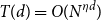$T(d) = O(N^{\eta d})$ , since ${\eta '} \leq \eta$ .

Before we analyse the full algorithm, we will make an observation about the function $g_n$ . In particular, we will require the following Lemma.

Lemma 24. For any vector of marginal probabilities ${\textrm{x}}$ , we have

\begin{equation*}g_n({{\textrm{x}}}) \geq \frac {1}{\sqrt {2}N},\end{equation*}

as long as the underlying hypergraph $G$ is connected.

Proof. So long as the input vector $\textbf {x}$ forms a probability distribution, we use equation (20) to see

\begin{align*} g_n({\textbf {x}}) &= \frac {\sum \limits _{n_1, \ldots n_{\eta '} \in [0,N-1]} \prod \limits _{j=1}^{\eta '} x^j(\bar n_j) \prod \limits _{e \in E, v \in e} \Phi _{e}(n, {\textrm{n}}_{e\setminus v})} {\sum \limits _{n_0, n_1, \ldots n_{\eta '} \in [0,N-1]} \prod \limits _{j=1}^{\eta '} x^j(\bar n_j) \prod \limits _{e \in E, v \in e} \Phi _{e}({\textrm{n}}_e)}\\[3pt] &\geq \frac {\sum \limits _{n_1, \ldots n_{\eta '} \in [0,N-1]} \prod \limits _{j=1}^{\eta '} x^j(\bar n_j) \prod \limits _{e \in E, v \in e} c_e} {\sum \limits _{n_0, n_1, \ldots n_{\eta '} \in [0,N-1]} \prod \limits _{j=1}^{\eta '} x^j(\bar n_j) \prod \limits _{e \in E, v \in e} c_e \left (1 + \frac {\log (1 + \frac {1}{\eta })}{2 \Delta }\right )}\\[3pt] &\geq \frac {\sum \limits _{n_1, \ldots n_{\eta '} \in [0,N-1]} \prod \limits _{j=1}^{\eta '} x^j(\bar n_j)} {\left (1 + \frac {\log (1 + \frac {1}{\eta })}{2 \Delta }\right )^\Delta \sum \limits _{n_0, n_1, \ldots n_{\eta '} \in [0,N-1]} \prod \limits _{j=1}^{\eta '} x^j(\bar n_j) }\\[3pt] &= \frac {1}{N \left (1 + \frac {\log (1 + \frac {1}{\eta })}{2 \Delta }\right )^\Delta }, \end{align*}

where the first inequality follows from the assumption in equation (7), the second inequality follows from $v$ being a member of at most $\Delta$ edges, and the final equality follows from equation (19). Further, we can observe that

\begin{equation*}\left (1 + \frac {\log (1 + \frac {1}{\eta })}{2 \Delta }\right )^\Delta \leq \exp \left (\log \left (1 + \frac {1}{\eta }\right )/2\right ) = \sqrt {1 + \frac {1}{\eta }} \leq \sqrt {2}, \end{equation*}

so long as the hypergraph is connected. Thus,

\begin{align*}g_n({\textbf {x}}) \geq \frac {1}{\sqrt {2}N}. \\[-24pt] \end{align*}

With this Lemma, we conclude with the following theorem.

Algorithm 4

ApproxZ’

Algorithm 4 Long description

An equation describing the estimation of the partition function of a hypergraph. The equation starts with the fraction with numerator one minus O(1/m) and denominator one, less than or equal to the fraction with numerator Z tilde(G) and denominator Z(G), less than or equal to one plus O(1/m). The equation is part of a proof that discusses the approximation of the partition function using an algorithm.

Theorem 25. The estimate $\tilde Z(G)$ of $Z(G)$ produced by algorithm 4 will satisfy

\begin{equation*}1 - O(1/m) \leq \frac {\tilde Z(G)}{Z(G)} \leq 1 + O(1/m)\end{equation*}

for some $d = O(\log (Nm))$ . This estimate will be computed in time $N^{O(\eta \log ( N m))}$ .

Proof. Order the vertices $v_1$ to $v_m$ in the same order they are iterated in algorithm4, and let $\beta _i = (v_j \leftarrow 0, j \leq i)$ as in the end of Section 2. Set 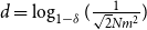$d = \log _{1 - \delta }(\frac {1}{\sqrt {2}Nm^2})$ . This will result in our approximations $y(G, v_i \leftarrow 0, \beta _{i-1})$ computed in the algorithm to satisfy

\begin{equation*}| x(G, v_i \leftarrow 0, \beta _{i-1}) - y(G, v_i \leftarrow 0, \beta _{i-1})| \leq (1 - \delta )^d = \frac {1}{\sqrt {2}Nm^2} \leq \frac {y(G, v_i \leftarrow 0, \beta _{i-1})}{m^2}\end{equation*}

by Lemma 23 and 24. Dividing both sides by $y(G, v_i \leftarrow 0, \beta _{i-1})$ , we get

\begin{equation*}\bigg | \frac { x(G, v_i \leftarrow 0, \beta _{i-1})}{y(G, v_i \leftarrow 0, \beta _{i-1})} - 1 \bigg | \leq \frac {1}{m^2}. \end{equation*}

Next, notice that

\begin{equation*}\frac {\tilde Z(G)}{Z(G)} = \frac {p(\textbf {0}) \prod \limits _{i = 1}^{n} y^{-1}(G, v_i \leftarrow 0)}{p(\textbf {0}) \prod \limits _{i = 1}^{n} x^{-1}(G, v_i \leftarrow 0)} = \frac {\prod \limits _{i = 1}^{n} x(G, v_i \leftarrow 0)}{\prod \limits _{i = 1}^{n} y(G, v_i \leftarrow 0)},\end{equation*}

by equation (9). Therefore, the estimate $\tilde Z$ produced by algorithm4 will satisfy

\begin{equation*}\left (1- \frac {1}{m^2}\right )^m = 1 - O(1/m) \leq \frac {\tilde Z(G)}{Z(G)} \leq 1 + O(1/m) \leq \left (1 + \frac {1}{m^2}\right )^m.\end{equation*}

The runtime of this algorithm will be dominated by the calls to the function ApproxProb’, which each take time $O(N^{\eta d})$ by Lemma 23. Further, notice that $d = O(\log (Nm))$ since $(1 - \delta ) \lt 1$ . Thus, since there are $m$ calls to this function with this $d$ , the algorithm will take time $N^{O(\eta \log ( Nm))}$ .

4.4 From discrete to continuous approximations

In this section, we will present one method for relating the value of a Riemann sum to the value of the corresponding integral, based on bounding the functions $l2$ -norm. This process will conclude with a short proof of theorem3.

Lemma 26. Suppose we have a function $f$ defined as in equation ( 5 ), where each function $\Phi _e$ is differentiable and satisfies $\|\nabla \Phi _e({{\textrm{x}}})\|_2 \leq kc_e$ for every ${{\textrm{x}}} \in [0,1]^m$ . Then,

\begin{equation*}\left ( 1 - \frac {\sqrt {m}k}{N} \right )^{|E|} \leq \frac {\int 1({\textrm{n}} \in [0,1]^m) p({\textrm{n}}) d\lambda }{Z(G)/N^m} \leq \left ( 1 + \frac {\sqrt {m}k}{N} \right )^{|E|} ,\end{equation*}

where $Z(G)$ is defined as in equation ( 6 ).

Proof. Pick any vector ${\textrm{n}} \in {\mathcal{D}}$ , and let ${\textrm{n}}'$ be any vector satisfying $n_i \leq n_i' \lt n_i + 1/N$ for each index $i$ . We will denote the set of all such ${\textrm{n}}'$ as ${\mathcal{D}}_{{\textrm{n}}}$ . Notice that 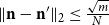$\|{\textrm{n}} - {\textrm{n}}'\|_2 \leq \frac {\sqrt {m}}{N}$ . Thus, for every edge $e \in E$ , we have

\begin{equation*}\Phi _e({\textrm{n}}) - \frac {\sqrt {m}}{N} k c_e \leq \Phi _e({\textrm{n}}') \leq \Phi _e({\textrm{n}}) + \frac {\sqrt {m}}{N}kc_e. \end{equation*}

Using this, we see

\begin{align*} \frac {\int _{{\mathcal{D}}_{{\textrm{n}}}} p({\textbf {x}}) d{\textbf {x}}}{p({\textrm{n}})/N^m} \leq \frac {\int _{{\mathcal{D}}_{{\textrm{n}}}} \prod \limits _{e \in E} \left (\Phi _e({\textrm{n}}) + \frac {\sqrt {m}}{N}kc_e d{\textbf {x}} \right )}{\prod \limits _{e \in E} \Phi _e({\textrm{n}})/N^m} = \frac {\prod \limits _{e \in E}\left (\Phi _e({\textrm{n}}) + \frac {\sqrt {m}}{N}kc_e\right )}{\prod \limits _{e\in E} \Phi _e({\textrm{n}})} \leq \left ( 1 + \frac {\sqrt {m}k}{N} \right )^{|E|}, \end{align*}

where the first inequality follows from the above equation, and the second inequality follows from the assumption in equation (7). Similar reasoning will yield that 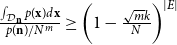$\frac {\int _{{\mathcal{D}}_{{\textrm{n}}}} p({\textbf {x}}) d{\textbf {x}}}{p({\textrm{n}})/N^m} \geq \bigg ( 1 - \frac {\sqrt {m}k}{N} \bigg )^{|E|}$ . Finally, we observe that

\begin{equation*}\frac {\int 1({\textrm{n}} \in [0,1]^m) p({\textrm{n}}) d\lambda }{Z(G)/N^m} = \frac {\sum \limits _{{\textrm{n}} \in {\mathcal{D}}} \int _{{\mathcal{D}}_{{\textrm{n}}}} p({\textbf {x}}) d{\textbf {x}}}{\sum \limits _{{\textrm{n}} \in {\mathcal{D}}} p({\textrm{n}})/N^m} \leq \max _{{\textrm{n}} \in {\mathcal{D}}} \frac {\int _{{\mathcal{D}}_{{\textrm{n}}}} p({\textbf {x}}) d{\textbf {x}}}{p({\textrm{n}})/N^m} \leq \left ( 1 + \frac {\sqrt {m}k}{N} \right )^{|E|},\end{equation*}

with similar logic yielding

\begin{equation*}\frac {\int 1({\textrm{n}} \in [0,1]^m) p({\textrm{n}}) d\lambda }{Z(G)/N^m} \geq \left ( 1 - \frac {\sqrt {m}k}{N} \right )^{|E|}.\end{equation*}

We are now ready to prove our second main result.

Proof of Theorem3

Let $N = k m^{3/2} |E|$ . By Lemma 26, we will have that

\begin{equation*}e^{-1/m} \leq \frac {\int 1({\textrm{n}} \in [0,1]^m) p({\textrm{n}}) d\lambda }{Z(G)/N^m} \leq e^{1/m},\end{equation*}

implying that

\begin{equation*}1 - O(1/m) \leq \frac {Z(G)/N^m}{\int 1({\textrm{n}} \in [0,1]^m) p({\textrm{n}}) d\lambda } \leq 1 + O(1/m).\end{equation*}

Now, let $\tilde Z(G)$ be the estimate of $Z(G)$ produced by algorithm4 when $d = O(\log (Nm)) = O(\log (m k |E|))$ . By theorem25, we must have that

\begin{equation*}1 - O(1/m) \leq \frac {\tilde Z(G)}{Z(G)} \leq 1 + O(1/m).\end{equation*}

Finally, we observe that

\begin{equation*}\left (\frac {Z(G)/N^m}{\int 1({\textrm{n}} \in [0,1]^m) p({\textrm{n}}) d\lambda }\right )\left (\frac {\tilde Z(G)}{Z(G)}\right ) = \frac {\tilde Z(G)/N^m}{\int 1({\textrm{n}} \in [0,1]^m) p({\textrm{n}}) d\lambda }, \end{equation*}

which means

\begin{equation*}(1-O(1/m))^2 = 1 - O(1/m) \leq \frac {\tilde Z(G)/N^m}{\int 1({\textrm{n}} \in [0,1]^m) p({\textrm{n}}) d\lambda } \leq 1 + O(1/m) = (1 + O(1/m))^2.\end{equation*}

Thus, if we set our estimate of the integral $\tilde V = \tilde Z(G)/N^m$ , we will have that

\begin{equation*}\bigg | \frac {\tilde V}{\int 1({\textrm{n}} \in [0,1]^m) p({\textrm{n}}) d\lambda } - 1 \bigg | \leq O(1/m).\end{equation*}

Further, the runtime to compute this estimate will be dominated by the runtime of algorithm4. By Theorem25, this will be $(k m |E|)^{O( \eta \log ( k m |E|))}$ . Observing $|E| \leq \Delta m$ and taking $\eta$ , $k$ , and $\Delta$ to be constants, we get a runtime of $m^{O(\log m)}$ .