1. Introduction
Simultaneous Localization and Mapping (SLAM), as a key technology for mobile robot navigation, utilizes onboard sensors to perform localization and mapping in unknown environments. Visual odometry often struggles with accurate distance measurement under varying illumination [Reference Loo, Amiri, Mashohor, Tang and Zhang1, Reference Campos, Elvira, Rodríguez, Montiel and Tardós2], leading to instability in dynamic environments. LiDAR-based odometry overcomes this by providing direct distance measurements with high accuracy and robustness [Reference Fasiolo, Scalera and Maset3, Reference Cao, Zhu, Choset and Zhang4]. While mechanical LiDARs achieve wide horizontal field-of-view (FoV), their limited vertical angular coverage results in significant cost and size constraints. Solid-state LiDARs resolve these issues with compact size, lower cost, and enhanced stability [Reference Lin and Zhang5, Reference Lee, Jung, Yang and Kim6], driving their adoption in mobile robotics.
Despite the strong development potential of solid-state LiDARs, it also brings new challenges: (1) Unlike mechanical LiDARs, solid-state LiDARs feature a narrower horizontal FoV and an irregular scanning pattern, which may cause scene degradation [Reference Smith and Cheeseman, “7, Reference Hu, Zhou, Miao, Yuan and Liu8]. Consequently, existing localization algorithms designed for mechanical LiDARs exhibit insufficient accuracy when applied to solid-state LiDARs. While learning-based approaches show potential in addressing such sparse point cloud registration [Reference J.F. and R.9, Reference S, M, M, J and S10], their reliance on extensive training data and substantial computational resources introduces significant constraints. (2) 3D maps are commonly stored in linear mode [Reference Gutmann and Konolige11, Reference Cadena, Carlone, Carrillo, Latif, Scaramuzza, Neira, Reid and Leonard12], which consumes a lot of computing resources when adding or deleting point clouds. Traditional tree structure used for representing point cloud maps [Reference Guttman13] can result in a large number of memory copies when the data structure is expanded, leading to a heavy computational load that hinders real-time updates.
In this paper, we address these issues through three key novel approaches: sparse voxel structures for incremental updating, a faster sparse Voxelized Generalized Iterative Closest Point (VGICP) algorithm, and an enhanced tightly-coupled LiDAR-Inertial fusion method via the Gauss-Newton method. Specifically, our contributions are as follows:
-
1. This paper proposes a novel sparse voxel maps (SVM) storage method that incorporates new voxel information and an update function to address the problems mentioned above. After accumulating and downsampling LiDAR measurements, feature points can be incrementally added or deleted from the SVM using a novel hash function. Compared to map storage structures based on kd-tree, the time complexity of voxel searches in SVM is O(1), significantly enhancing the efficiency of map registration.
-
2. We use SVM-based local maps combined with the Generalized Iterative Closest Point (GIPC) method to achieve point cloud registration. This approach optimizes localization deviations caused by insufficient LiDAR feature points in small FoV scenarios and achieves better robustness in sparse point cloud environments, especially when great motion changes occur between frames.
-
3. We incorporate the above two key technologies into an enhanced tightly coupled LiDAR-inertial odometry (LIO) system. This system performs forward propagation via IMU measurement, followed by a rigorous back-propagation process to correct for the motion-induced distortion of each feature point. Ultimately, the system estimates its complete state through the Gauss-Newton method and updates the SVMs based on the feedback from these estimation results.
The remainder of this paper is organized as follows. In Section 2, we synthesize pertinent research studies. In Section 3, we provide an overview of the entire system pipeline. Sections 4, 5, and 6 detail the IMU state, LiDAR point cloud, and state estimation component, respectively. The experimental results are presented in Section 7. Finally, Section 8 concludes the paper.
2. Related work
2.1. Dynamic data structure in mapping
K-d tree [Reference Bentley14] and R*-tree [Reference Beckmann, Kriegel, Schneider and Seeger15] efficiently support k-nearest neighbor search for real-time mapping in two categories: data division and space splitting. The incremental k-d tree (ikd-Tree) used by FAST-LIO2 [Reference Xu, Cai, He, Lin and Zhang16] reduces the time to update data while maintaining real-time ability. Tree data structures could be improved to more compact forms for neighborhood search, such as the hashed voxel structure, which is a common alternative to hierarchical tree structure. For instance, LiTAMIN [Reference Yokozuka, Koide, Oishi and Banno17] divides the points into individual voxels and performs a normal distribution transformation within each voxel. FASTER-LIO [Reference Bai, Xiao, Chen, Wang, Zhang and Gao18] improves the data structure from ikd-Tree to iVox, further enhancing the algorithm’s speed to achieve more efficient odometry with the same level of accuracy. Compared to tree data structure, the voxelization method is not only easier to construct but also exhibits stable time complexity for modifications and deletions.
2.2. 3D point cloud registration
The existing LiDAR SLAM research works are extensive. For traditional spinning LiDARs, some low-latency methods, such as LoLa-SLAM [Reference Karimi, Oelsch, Stengel, Babaians and Steinbach19], utilize partial scan data for point cloud registration. However, these methods are primarily applicable to spinning LiDARs and present significant challenges when adapted to solid-state LiDARs.
The Iterative Closest Point (ICP) algorithm proposed by Besl et al. [Reference Besl and McKay20] estimates the corresponding pose between consecutive frames by minimizing the transformation error, but ICP tends to fall into local minima and has high initial positional requirements. The normal distributions transform (NDT) [Reference Biber and Strasser21] avoids point-to-point matching by creating normal distributions to align two point clouds, but NDT is sensitive to the choice of voxel resolution. Zhang et al. [Reference Zhang and Singh22] propose LOAM, which identifies bumps on edges and surfaces by evaluating the smoothness of the local planes and correcting point cloud registration. Common algorithms such as LOAM take about 100 ms to perform point cloud registration, but higher processing speeds must be achieved for solid-state LiDARs.
2.3. Tightly coupled LiDAR-inertial odometry
Compared to the loosely coupled approaches, where sensors calculate their states separately before fusing them, tightly coupled methods integrate data fusion during the sensor state computation process, achieving better performance in terms of robustness and accuracy. LILI-OM [Reference Li, Li and Hanebeck23] uses a lightweight LiDAR odometer in the front end to provide fast motion estimation for adaptive keyframes and optimizes the back end performs through a hierarchical sliding window based on keyframes. IN2LAMA [Reference Gentil, Vidal-Calleja and Huang24] utilizes the up-sampled IMU pre-integration to optimize the motion distortion, and designs a streaming optimization framework that includes the sensor time-shift factor, which effectively removes motion distortion but performs poorly in real-time applications. LIO-SAM [Reference Shan, Englot, Meyers, Wang, Ratti and Rus25] algorithm uses pre-integration estimation of IMU for both motion compensation and optimization in factorization maps, but it fails in degraded environments due to a lack of valid observations. With the development of high-frequency solid-state LiDARs, LIO requires higher computational efficiency. FAST-LIO [Reference Xu and Zhang26] addresses the computationally intensive problem by introducing a novel Kalman gain formulation, but it may not perform well when the point cloud is sparse or irregular and does not provide an efficient solution for reducing feature extraction consumption. Further, FAST-LIO2 [Reference Xu, Cai, He, Lin and Zhang16] avoids feature extraction procedure through the ikd-Tree data structure and directly matches scans with local maps, improving speed and accuracy, but ikd-Tree is not well-suited for constructing large-scale maps and can only maintain a specific range.
The system’s overall pipeline.

3. System overview
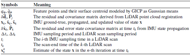
The overview of our framework is shown in Figure 1. The LiDAR inputs are first preprocessed, and then the undistorted LiDAR feature points and the IMU forward propagation state prediction values are used to compute the constraints. Subsequently, these constraints are locally optimized using the Gauss-Newton method for tight coupling. Finally, the optimally selected feature points are merged into the existing SVM, and the updated voxel map is utilized to register new feature points in the next step. In addition, we will use the notations summarized in Table I.
Notations.

4. IMU state propagation
4.1. IMU measurement model
In this paper, the first frame of IMU data is set as the global system. The state of the mobile robot
 $\mathbf{x}$
is defined as follows:
 \begin{equation} {\mathbf{x}}\ \dot =\ {\left [ {\begin{array}{c@{\quad}c@{\quad}c@{\quad}c@{\quad}c@{\quad}c@{\quad}c@{\quad}c} {^G{\mathbf{R}}_I^T}&{^G{\mathbf{p}}_I^T}&{^G{\mathbf{v}}_I^T}&{{\mathbf{b}}_{\mathbf{a}}^T}&{{\mathbf{b}}_{\boldsymbol{\omega }}^T}&{{}^G{{\mathbf{g}}^T}}&{^I{\mathbf{R}}_L^T}&{^I{\mathbf{p}}_L^T} \end{array}} \right ]^T} \end{equation}
where
 $^G{{\textbf {R}}_I} \in SO(3)$
and
 $^G{{\textbf {p}}_I} \in {\mathbb{R}^3}$
denote the IMU rotation matrix and position vector in the global frame,
 $^G{{\textbf {v}}_I} \in {\mathbb{R}^3}$
denotes IMU velocity vector in the global frame,
 $({}^I{{\textbf {R}}_L},{}^I{{\textbf {p}}_L}) \in SE(3)$
represents the known extrinsic transformation between LiDAR and IMU,
 ${{\mathbf{b}}_{\mathbf{a}}} \in {\mathbb{R}^3}$
and
 ${{\mathbf{b}}_{\boldsymbol{\omega }}} \in {\mathbb{R}^3}$
are the IMU biases modeled as random walk process, and
 ${}^G{\mathbf{g}}\in {\mathbb{R}^3}$
is the gravity vector in the global frame.
Based on continuous model [Reference Xu, Cai, He, Lin and Zhang16, Reference Xu and Zhang26] and encapsulation operators
 $ \oplus$
,
 $ \ominus$
[Reference Hertzberg, Wagner, Frese and Schröder27], we can discretize the state at the IMU sampling period
 $\Delta {t_i}$
. During a LiDAR scan sampling period
 $\Delta {t_k}$
, there are multiple IMU measurements, each sampled at time
 ${t_i} \in [{t_{k - 1}},{t_k}]$
with the respective state
 ${\mathbf{x}}_i$
as follows:
 \begin{equation} {{\mathbf{x}}_{i + 1}} = {{\mathbf{x}}_i} \oplus ({\mathbf{f}}({{\mathbf{x}}_i},{{\mathbf{u}}_i},{{\mathbf{w}}_i})\Delta {t_i}) \end{equation}
where
 $i$
is the index of IMU measurements, and
 ${\mathbf{x}}_i$
,
 ${\mathbf{u}}_i$
,
 ${\mathbf{w}}_i$
are the ground-true values of the state, input, and noise at
 $i$
-th IMU sampling time. These values are defined by IMU measurement model as follows:
 \begin{align} {\mathbf{u}} &\doteq {\left [ {\begin{array}{c@{\quad}c} {{{\mathbf{a}}^T}}&{{{\boldsymbol{\omega }}^T}} \end{array}} \right ]^T},{\mathbf{w}}{\text{ }} \!\doteq \! {\left [ {\begin{array}{c@{\quad}c@{\quad}c@{\quad}c} {{\mathbf{n}}_{\mathbf{a}}^T}&{{\mathbf{n}}_{\boldsymbol{\omega }}^T}&{{\mathbf{n}}_{{\mathbf{ba}}}^T}&{{\mathbf{n}}_{{\mathbf{b}{\boldsymbol{\omega }}}}^T} \end{array}} \right ]^T} \nonumber\\[6pt] {\mathbf{f}}({\mathbf{x}},{\mathbf{u}},{\mathbf{w}}) &= \left [ {\begin{array}{c} {{\boldsymbol{\omega }} - {{\mathbf{b}}_{\boldsymbol{\omega }}} - {{\mathbf{n}}_{\boldsymbol{\omega }}}} \\ {^G{{\mathbf{v}}_I} + \frac {1}{2}{(^G}{{\mathbf{R}}_I}({\mathbf{a}} - {{\mathbf{b}}_{\mathbf{a}}} - {{\mathbf{n}}_{\mathbf{a}}}) + {}^G{\mathbf{g}})\Delta t} \\ {^G{{\mathbf{R}}_I}({\mathbf{a}} - {{\mathbf{b}}_{\mathbf{a}}} - {{\mathbf{n}}_{\mathbf{a}}}) + {}^G{\mathbf{g}}} \\ {{{\mathbf{n}}_{{\mathbf{ba}}}}} \\ {{{\mathbf{n}}_{{\mathbf{b}{\boldsymbol{\omega }}}}}} \\ {{{\mathbf{0}}_{3 \times 1}}} \\ {{{\mathbf{0}}_{3 \times 1}}} \\ {{{\mathbf{0}}_{3 \times 1}}} \end{array}} \right ] \end{align}
where
 $\mathbf{a}$
and
 $\boldsymbol{\omega }$
are linear acceleration and angular velocity inputs from IMU measurements, and
 ${\mathbf{n}}_{\mathbf{a}}$
,
 ${\mathbf{n}}_{\boldsymbol{\omega }}$
,
 ${\mathbf{n}}_{{\mathbf{ba}}}$
,
 ${\mathbf{n}}_{{\mathbf{b}{\boldsymbol{\omega }}}}$
are white noise of IMU measurements.
4.2. Forward propagation
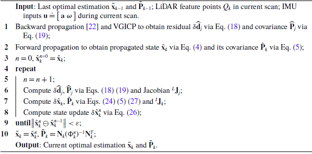
The update frequency is determined by the LiDAR scan sample time. Forward propagation is executed each time a new IMU input is received. As shown in Figure 2, IMU forward propagation is based on the last scan optimal estimate
 $\bar{\mathbf{x}}_{k\!-\!1}$
with covariance matrix
 $\bar{\mathbf{P}}_{k \!-\! 1}$
at time
 $t_{k \!-\! 1}$
and the IMU measurement between time
 $t_{k \!-\! 1}$
and
 $t_k$
, to obtain the propagated state
 $\hat{\mathbf{x}}_k$
and propagated covariance
 $\hat{\mathbf{P}}_k$
at time
 $t_k$
.
The forward and backward propagation.

Specifically, the propagated state follows the discrete model (2) by setting the noise
 ${\mathbf{w}}_i$
to zero:
 \begin{align}{\hat{\mathbf{x}}_{i + 1}} &= {\hat{\mathbf{x}}_i} \oplus ({\mathbf{f}}({\hat{\mathbf{x}}_i},{{\mathbf{u}}_i},{\mathbf{0}})\Delta {t_i});\,{\hat{\mathbf{x}}_0} = {\bar{\mathbf{x}}_k}\end{align}
 \begin{align}{\hat{\mathbf{P}}_{i + 1}} &= {{\mathbf{F}}_{\!\delta {{\mathbf{x}}_i}}}{\hat{\mathbf{P}}_i}{\mathbf{F}}_{\!\delta {{\mathbf{x}}_i}}^T \!+ {{\mathbf{F}}_{{{\mathbf{w}}_i}}}{{\mathbf{Q}}_i}{\mathbf{F}}_{{{\mathbf{w}}_i}}^T;\,{\hat{\mathbf{P}}_0} = {\bar{\mathbf{P}}_k}\end{align}
where
 $\hat{\mathbf{x}}_i$
is the propagated state prediction value at
 $i$
-th IMU sampling time,
 $\hat{\mathbf{P}}_i$
is the propagated covariance, and
 ${\mathbf{Q}}_i$
is the covariance of noise
 ${\mathbf{w}}_i$
. The calculation of matrix
 ${\mathbf{F}}_{\!\delta {{\mathbf{x}}_i}}$
and
 ${\mathbf{F}}_{{{\mathbf{w}}_i}}$
will be performed next.
To propagate the covariance while considering the error, we use the error state dynamic model obtained below:
 \begin{equation} \begin{aligned} \delta {{\hat{\mathbf{x}}}_{i + 1}} &= {{\mathbf{x}}_{i + 1}} \ominus {{\hat{\mathbf{x}}}_{i + 1}} \\ &= ({{\mathbf{x}}_i} \oplus ({\mathbf{f}}({{\mathbf{x}}_i},\!{{\mathbf{u}}_i},\!{{\mathbf{w}}_i})\Delta {t_i})) \ominus ({{\hat{\mathbf{x}}}_i} \oplus ({\mathbf{f}}({{\hat{\mathbf{x}}}_i},\!{{\mathbf{u}}_i},\!{\mathbf{0}})\Delta {t_i})) \\ &\approx {{\mathbf{F}}_{\!\delta {\mathbf{x}}}}\delta {{\mathbf{x}}_i} + {{\mathbf{F}}_{{{\mathbf{w}}_i}}}{{\mathbf{w}}_i} \end{aligned} \end{equation}
From dynamic model in Eq. (6), it can be deduced that
 ${{\textbf {x}}_i} = {\hat{\mathbf{x}}_i} \oplus \delta {\hat{\mathbf{x}}_i}$
. Then we define
 ${\mathbf{g}}(\delta {{\mathbf{x}}_i},{{\mathbf{w}}_i}) = {\mathbf{f}}({{\mathbf{x}}_i},{{\mathbf{u}}_i},{{\mathbf{w}}_i})\Delta {t_i} = {\mathbf{f}}({\hat{\mathbf{x}}_i} \oplus \delta {{\mathbf{x}}_i},{{\mathbf{u}}_i},{{\mathbf{w}}_i})\Delta {t_i}$
, thus the error state dynamic model (6) can be rewritten as:
 \begin{equation} \begin{aligned} \delta {{\mathbf{x}}_{i + 1}} &= (({{\hat{\mathbf{x}}}_i} \oplus \delta {{\mathbf{x}}_i}) \oplus {\mathbf{g}}(\delta {{\mathbf{x}}_i},{{\mathbf{w}}_i})) \ominus ({{\hat{\mathbf{x}}}_i} \oplus {\mathbf{g}}({\mathbf{0}},{\mathbf{0}})) \\ &\doteq {\mathbf{G}}(\delta {{\mathbf{x}}_i},{\mathbf{g}}(\delta {{\mathbf{x}}_i},{{\mathbf{w}}_i})) \\ \end{aligned} \end{equation}
Following the chain rule for partial differentials, matrices
 ${\mathbf{F}}_{\!\delta {{\mathbf{x}}_i}}$
and
 ${\mathbf{F}}_{{{\mathbf{w}}_i}}$
are computed as follows:
 \begin{equation} \begin{aligned} &{{\textbf {F}}_{\!\delta {{\hat{\mathbf{x}}}_i}}} = {\left . {\frac {{\partial {\textbf {G}}\!\left ( {\delta {{\textbf {x}}_i},{\textbf {g}}\left ( {\delta {{\textbf {x}}_i},{\textbf {0}}} \right )} \right )}}{{\partial \!\left ( {\delta {{\textbf {x}}_i}} \right )}}} \right |_{\delta {{\hat{\mathbf{x}}}_i} = {\textbf {0}}}} = {\left . {\left ( {\frac {{\partial {\textbf {G}}\!\left ( {\delta {{\textbf {x}}_i},{\textbf {g}}({\textbf {0}},{\textbf {0}})} \right )}}{{\partial \!\left ( {\delta {{\textbf {x}}_i}} \right )}} + \frac {{\partial {\textbf {G}}\!\left ( {{\textbf {0}},{\textbf {g}}\!\left ( {\delta {{\textbf {x}}_i},{\textbf {0}}} \right )} \right )}}{{\partial {\textbf {g}}\!\left ( {\delta {{\textbf {x}}_i},{\textbf {0}}} \right )}}\frac {{\partial {\textbf {g}}\!\left ( {\delta {{\textbf {x}}_i},{\textbf {0}}} \right )}}{{\partial \!\left ( {\delta {{\textbf {x}}_i}} \right )}}} \right )} \right |_{\delta {{\hat{\mathbf{x}}}_i} = {\textbf {0}}}}\\[5pt] &{{\textbf {F}}_{{{\textbf {w}}_i}}} = {\left . {\frac {{\partial {\textbf {G}}\!\left ( {{\textbf {0}},{\textbf {g}}\!\left ( {{\textbf {0}},{{\textbf {w}}_i}} \right )} \right )}}{{\partial {{\textbf {w}}_i}}}} \right |_{{{\textbf {w}}_i} = {\textbf {0}}}} = {\left . {\left ( {\frac {{\partial {\textbf {G}}\!\left ( {{\textbf {0}},{\textbf {g}}\!\left ( {{\textbf {0}},{{\textbf {w}}_i}} \right )} \right )}}{{\partial {\textbf {g}}\!\left ( {{\textbf {0}},{{\textbf {w}}_i}} \right )}}\frac {{\partial {\textbf {g}}\!\left ( {{\textbf {0}},{{\textbf {w}}_i}} \right )}}{{\partial {{\textbf {w}}_i}}}} \right )} \right |_{{{\textbf {w}}_i} = {\textbf {0}}}} \end{aligned} \end{equation}
The partial differentials in Eq. (8) are computed in Eq. (9), where
 ${{\boldsymbol{\hat \omega }}_i} = {{\boldsymbol{\tilde \omega }}_i} - {\hat{\mathbf{b}}_{{{\boldsymbol{\omega }}_i}}}$
,
 ${\hat{\mathbf{a}}_i} = {\tilde{\mathbf{a}}_i} - {\hat{\mathbf{b}}_{{{\mathbf{a}}_i}}}$
.
 \begin{align*} \frac {{\partial {\textbf {G}}\!\left ( {\delta {{\textbf {x}}_i},{\textbf {g}}({\textbf {0}},{\textbf {0}})} \right )}}{{\partial \! \left ( {\delta {{\textbf {x}}_i}} \right )}} &= \left [ {\begin{array}{c@{\quad}c} {{\mathop {\textrm {Exp}}\nolimits } \left ( { - {{{\boldsymbol{\hat \omega }}}_i}\Delta t} \right )}&{\textbf {0}}\\ {\textbf {0}}&{{{\textbf {I}}_{21}}} \end{array}} \right ]\nonumber\\[5pt] \frac {{\partial {\textbf {G}}\!\left ( {{\textbf {0}},{\textbf {g}}\left ( {\delta {{\textbf {x}}_i},{\textbf {0}}} \right )} \right )}}{{\partial {\textbf {g}}\!\left ( {\delta {{\textbf {x}}_i},{\textbf {0}}} \right )}} &= \frac {{\partial {\textbf {G}}\!\left ( {{\textbf {0}},{\textbf {g}}\left ( {{\textbf {0}},{{\textbf {w}}_i}} \right )} \right )}}{{\partial {\textbf {g}}\!\left ( {{\textbf {0}},{{\textbf {w}}_i}} \right )}} = \left [ {\begin{array}{c@{\quad}c} {{\textbf {A}}{{\left ( {{{{\boldsymbol{\hat \omega }}}_i}\Delta t} \right )}^T}}&{\textbf {0}}\\ {\textbf {0}}&{{{\textbf {I}}_{21}}} \end{array}} \right ]\end{align*}
 \begin{align}\frac {{\partial {\textbf {g}}\!\left ( {\delta {{\textbf {x}}_i},{\textbf {0}}} \right )}}{{\partial \!\left ( {\delta {{\textbf {x}}_i}} \right )}} &= \frac {{\partial {\textbf {f}}\!\left ( {{{\hat{\mathbf{x}}}_i} \oplus \delta {{\textbf {x}}_i},{{\textbf {u}}_i},{\textbf {0}}} \right )}}{{\partial \!\left ( {\delta {{\textbf {x}}_i}} \right )}}\Delta t = \left [ {\begin{array}{c@{\quad}c@{\quad}c@{\quad}c@{\quad}c@{\quad}c@{\quad}c@{\quad}c} {\textbf {0}}&{\textbf {0}}&{\textbf {0}}&{ - {{\textbf {I}}_3}}&{\textbf {0}}&{\textbf {0}}&{\textbf {0}}&{\textbf {0}}\\ {\textbf {0}}&{\textbf {0}}&{{{\textbf {I}}_3}}&{\textbf {0}}&{\textbf {0}}&{\textbf {0}}&{\textbf {0}}&{\textbf {0}}\\ {{ - ^G}{{\widehat {\textbf {R}}}_{{I_i}}}{{[{{\hat{\mathbf{a}}}_i}]}^ \wedge }}&{\textbf {0}}&{\textbf {0}}&{\textbf {0}}&{{ - ^G}{{\widehat {\textbf {R}}}_{{I_i}}}}&{{{\textbf {I}}_3}}&{\textbf {0}}&{\textbf {0}}\\ {\textbf {0}}&{\textbf {0}}&{\textbf {0}}&{\textbf {0}}&{\textbf {0}}&{\textbf {0}}&{\textbf {0}}&{\textbf {0}}\\ {\textbf {0}}&{\textbf {0}}&{\textbf {0}}&{\textbf {0}}&{\textbf {0}}&{\textbf {0}}&{\textbf {0}}&{\textbf {0}}\\ {\textbf {0}}&{\textbf {0}}&{\textbf {0}}&{\textbf {0}}&{\textbf {0}}&{\textbf {0}}&{\textbf {0}}&{\textbf {0}}\\ {\textbf {0}}&{\textbf {0}}&{\textbf {0}}&{\textbf {0}}&{\textbf {0}}&{\textbf {0}}&{\textbf {0}}&{\textbf {0}}\\ {\textbf {0}}&{\textbf {0}}&{\textbf {0}}&{\textbf {0}}&{\textbf {0}}&{\textbf {0}}&{\textbf {0}}&{\textbf {0}} \end{array}} \right ]\!\Delta t\nonumber\\[5pt] \frac {{\partial {\textbf {g}}\!\left ( {{\textbf {0}},{{\textbf {w}}_i}} \right )}}{{\partial {{\textbf {w}}_i}}} &= \frac {{\partial {\textbf {f}}\!\left ( {{{\hat{\mathbf{x}}}_i},{{\textbf {u}}_i},{{\textbf {w}}_i}} \right )}}{{\partial {{\textbf {w}}_i}}}\Delta t = \left [ {\begin{array}{c@{\quad}c@{\quad}c@{\quad}c} { - {{\textbf {I}}_3}}&{\textbf {0}}&{\textbf {0}}&{\textbf {0}}\\ {\textbf {0}}&{\textbf {0}}&{\textbf {0}}&{\textbf {0}}\\ {\textbf {0}}&{{ - ^G}{{\widehat {\textbf {R}}}_{{I_i}}}}&{\textbf {0}}&{\textbf {0}}\\ {\textbf {0}}&{\textbf {0}}&{{{\textbf {I}}_3}}&{\textbf {0}}\\ {\textbf {0}}&{\textbf {0}}&{\textbf {0}}&{{{\textbf {I}}_3}}\\ {\textbf {0}}&{\textbf {0}}&{\textbf {0}}&{\textbf {0}}\\ {\textbf {0}}&{\textbf {0}}&{\textbf {0}}&{\textbf {0}}\\ {\textbf {0}}&{\textbf {0}}&{\textbf {0}}&{\textbf {0}} \end{array}} \right ]\!\Delta t \end{align}
where
 $[\mathbf{u}]^ \wedge$
denotes the skew-symmetric matrix of vector
 ${\mathbf{u}} \in {\mathbb{R}^3}$
.
 $\mathbf{A}(\mathbf{u})^{-1}$
is the inverse right Jacobian of
 $SO(3)$
, mapping rotation matrices
 $\mathbf{R} \in SO(3)$
to their corresponding Lie algebra representations
 $[\mathbf{u}]^\wedge$
:
 \begin{equation} {\textbf {A}}{(\mathbf{u})^{ - 1}} = {\textbf {I}} - \frac {1}{2}{[\mathbf{u}]^ \wedge } + \left ( {1 - \frac {{\left \| \mathbf{u} \right \|}}{2}\cot \frac {{\left \| \mathbf{u} \right \|}}{2}} \right )\frac {{{{\left ( {{{[\mathbf{u}]}^ \wedge }} \right )}^2}}}{{{{\left \| \mathbf{u} \right \|}^2}}} \end{equation}
Substituting Eq. (9) into Eq. (8) gives:
 \begin{align} &{{\textbf {F}}_{\!\delta {{\textbf {x}}_i}}} = \left [ {\begin{array}{c@{\quad}c@{\quad}c@{\quad}c@{\quad}c@{\quad}c@{\quad}c@{\quad}c} {{\rm {Exp}}\left ( { - {{{\boldsymbol{\hat \omega }}}_i}\Delta t} \right )}&{\textbf {0}}&{\textbf {0}}&{ - {\textbf {A}}{{\left ( {{{{\boldsymbol{\hat \omega }}}_i}\Delta t} \right )}^T}\Delta t}&{\textbf {0}}&{\textbf {0}}&{\textbf {0}}&{\textbf {0}}\\ {\textbf {0}}&{\textbf {I}}&{{\textbf {I}}\Delta t}&{\textbf {0}}&{\textbf {0}}&{\textbf {0}}&{\textbf {0}}&{\textbf {0}}\\ {{ - ^G}{{\widehat {\textbf {R}}}_{{I_i}}}{{[{{\hat{\mathbf{a}}}_i}]}^ \wedge }\Delta t}&{\textbf {0}}&{\textbf {I}}&{\textbf {0}}&{{ - ^G}{{\widehat {\textbf {R}}}_{{I_i}}}\Delta t}&{{\textbf {I}}\Delta t}&{\textbf {0}}&{\textbf {0}}\\ {\textbf {0}}&{\textbf {0}}&{\textbf {0}}&{\textbf {I}}&{\textbf {0}}&{\textbf {0}}&{\textbf {0}}&{\textbf {0}}\\ {\textbf {0}}&{\textbf {0}}&{\textbf {0}}&{\textbf {0}}&{\textbf {I}}&{\textbf {0}}&{\textbf {0}}&{\textbf {0}}\\ {\textbf {0}}&{\textbf {0}}&{\textbf {0}}&{\textbf {0}}&{\textbf {0}}&{\textbf {I}}&{\textbf {0}}&{\textbf {0}}\\ {\textbf {0}}&{\textbf {0}}&{\textbf {0}}&{\textbf {0}}&{\textbf {0}}&{\textbf {0}}&{\textbf {I}}&{\textbf {0}}\\ {\textbf {0}}&{\textbf {0}}&{\textbf {0}}&{\textbf {0}}&{\textbf {0}}&{\textbf {0}}&{\textbf {0}}&{\textbf {I}} \end{array}} \right ]\nonumber \\[5pt] &{{\textbf {F}}_{{{\textbf {w}}_i}}}{\rm { }} = \left [ {\begin{array}{c@{\quad}c@{\quad}c@{\quad}c} { - {\textbf {A}}{{\left ( {{{{\boldsymbol{\hat \omega }}}_i}\Delta t} \right )}^{\rm {T}}}\Delta t}&{\textbf {0}}&{\textbf {0}}&{\textbf {0}}\\ {\textbf {0}}&{\textbf {0}}&{\textbf {0}}&{\textbf {0}}\\ {\textbf {0}}&{{ - ^G}{{\widehat {\textbf {R}}}_{{I_i}}}\Delta t}&{\textbf {0}}&{\textbf {0}}\\ {\textbf {0}}&{\textbf {0}}&{{\textbf {I}}\Delta t}&{\textbf {0}}\\ {\textbf {0}}&{\textbf {0}}&{\textbf {0}}&{{\textbf {I}}\Delta t}\\ {\textbf {0}}&{\textbf {0}}&{\textbf {0}}&{\textbf {0}}\\ {\textbf {0}}&{\textbf {0}}&{\textbf {0}}&{\textbf {0}}\\ {\textbf {0}}&{\textbf {0}}&{\textbf {0}}&{\textbf {0}} \end{array}} \right ] \end{align}
After the propagated state
 $\hat{\mathbf{x}}_i$
is updated by multiple IMU measurements, the forward propagation continues until reaching the end time of the scan
 $t_k$
. Thus, we obtain the propagated state
 $\hat{\mathbf{x}}_k$
and propagated covariance
 $\hat{\mathbf{P}}_k$
at time
 $t_k$
through state propagation Eqs. (4) and (5).
5. LiDAR point cloud registration
The point cloud registration process is illustrated in Figure 3. The algorithm begins with preprocessing, undistortion, and voxel covariance estimation. Subsequently, the point cloud is aligned with the sub-map based on the number of point cloud frames. During the initial stage, when the local map is sparse, direct local map updating or scan-to-map matching methods [Reference Segal, Hähnel and Thrun28] are employed. Once the point cloud data in the local map become dense, the VGICP algorithm [Reference Koide, Yokozuka, Oishi and Banno29] is utilized for point cloud registration to derive LiDAR constraints. These LiDAR constraints are subsequently utilized for real-time localization, and the updated pose is employed to refine the local map.
LiDAR point clouds registration pipeline.

5.1. Sparse voxel maps
We design a sparse voxel structure, which incorporates new voxel information and an update function to preserve feature point information and construct local maps
 $M$
during LiDAR scanning. Each voxel in the SVMs is designed as:
 \begin{equation} {V_m} = [\begin{array}{c@{\quad}c@{\quad}c@{\quad}c} {{N_m}^T}&{{U_m}^T}&{{O_m}^T}&{{C_m}^T} \end{array}] \end{equation}
where
 ${V_m} \in M$
,
 $m \in [0,{s_M}]$
represents the
 $m$
-th sparse voxel in the local map,
 $s_M$
is the total number of sparse voxels in the local map, determining the hash table size,
 $N_m$
is the number of feature points contained in this voxel,
 $U_m$
is the sum of the 3D coordinates of all feature points in this voxel,
 $O_m$
is the sum of the outer products of the feature points contained in this voxel, and
 $C_m$
is the covariance of this voxel.
The point cloud is sparse and unordered. Using an ordered array storage structure would waste storage space; therefore, we employ an unordered hash map to store the sparse voxels that contain at least one point. The hash index is computed by discretizing the feature point coordinates into voxel grid indices and applying a hash function:
 \begin{align}{{\textbf {h}}_V} &= {[\begin{array}{c@{\quad}c@{\quad}c} {{h_x}}&{{h_y}}&{{h_z}} \end{array}]^T} = {\left [ {\begin{array}{c@{\quad}c@{\quad}c} {{\rm {floor}}\left(\frac {{{p_x}}}{{{s_V}}}\right)}&{{\rm {floor}}\left(\frac {{{p_y}}}{{{s_V}}}\right)}&{{\rm {floor}}\left(\frac {{{p_z}}}{{{s_V}}}\right)} \end{array}} \right ]^T}\nonumber\\ i{d_V} &= {\rm {hash}}({{\textbf {h}}_V}) = ({h_x}{n_x}){\rm {xor}}({h_y}{n_y}){\rm {xor}}({h_z}{n_z})\!\!\,\bmod \,\!\!{s_M}\end{align}
where
 $p_x$
,
 $p_y$
,
 $p_z$
are the coordinates of feature point,
 $s_V$
is the voxel size, defining the spatial resolution of the voxel grid,
 ${\rm {floor}}(x)$
represents the greatest integer less than or equal to
 $x$
, and
 $n_x$
,
 $n_y$
,
 $n_z$
are large prime numbers. Obviously, we added a
 ${\rm {floor}}(x)$
function to the hash function mentioned above to reduce the computational consumption. This discretization converts continuous coordinates to integer voxel indices for efficient spatial indexing. Prime-based hashing ensures uniform distribution of
 $id_V$
, while the modulo operation constrains memory consumption –
 $s_V$
governs spatial resolution and
 $s_M$
specifies the maximum sparse voxels in the local map.
The incremental map update involves the insertion and deletion of voxels. Before point insertions, we downsample the point using Voxel-Grid filter to maintain the shape features of the point cloud while reducing unnecessary points. After downsampling, we use the hash function (13) to compute the hash index of the feature point
 $q_m$
, and incrementally add
 $q_m$
into the matching sparse voxels
 $V_m$
. The updates to
 $N_m$
,
 $U_m$
,
 $O_m$
,
 $C_m$
are shown in Eq. (14). Finally, the updated voxels are integrated into SVM.
 \begin{align}N'\!_{m} &= {N_m} + {\tilde N}_{m}\nonumber\\[3pt]U'\!_{m} &= {U_m} + {\tilde U}_{m}\nonumber\\[3pt]O'\!_{m} &= {O_m} + {\tilde O}_{m}\\[3pt]{{C'}\!_m} &= \frac {1}{{{{N'}\!_m}}} \left [\begin{array}{c} {{{O'}\!_m} - {{U'}\!_m} \cdot {{\left(\dfrac {{{U_m}}}{{{N_m}}}\right)}^T}}\nonumber\\ \end{array}\right ]\end{align}
The above update function enhances the efficiency and accuracy of map updates and point cloud registration through the use of
 $O_m$
elements and a novel covariance update calculation method. Meanwhile, this paper employs the Least Recently Used (LRU) cache strategy [Reference O’Neil, O’Neil and Weikum30] to achieve incremental deletion. The LRU maintains a queue of recently visited voxels and deletes the least used voxels, which can avoid data redundancy as the map expands.
5.2. Voxelized GICP
To achieve LIO, LiDAR is required to perform point cloud registration to compute the transformation between two consecutive frames. This section further combines the SVMs with GICP algorithm [Reference Segal, Hähnel and Thrun28] to implement incremental point cloud registration.
The sampling rate of the LiDAR raw points is high (Livox Avia used in this paper has a sampling rate of at least 240 kHz). These raw points are accumulated over a 100 ms period (corresponding to a 10 Hz update rate). The accumulated point cloud is referred to as a LiDAR scan, and the period for sampling a LiDAR scan is denoted as
 $\Delta {t_k}$
.
We employ the backpropagation proposed in ref. [Reference Xu and Zhang26], which enables us to project all feature points (i.e. accumulated and downsampled LiDAR raw points) to the scan end time
 $t_k$
based on IMU measurements.
Assuming that the following steps have been completed, including LiDAR input preprocessing, undistortion, and covariance estimation. We now compute the transformation matrix
 ${\textbf {T}} \in SE(3)$
, which aligns the point cloud from the previous frame
 ${Q_{k \!-\! 1}} = \{ {q_0}, \ldots ,{q_j}\}$
with the point cloud from the next frame
 ${Q_k} = \{ {q_0}, \ldots ,{q_m}\}$
. We assume that the correspondences between point sets
 $Q_{k \!-\! 1}$
and
 $Q_k$
are determined using the nearest neighbor search:
 ${q_m} = {\textbf {T}}{q_j}$
. The GICP algorithm models the sampling surface of each feature point as a Gaussian distribution:
 ${q_m} \!\sim \! \mathcal{N}({\hat{q}_m},{C_m})$
,
 ${q_j} \!\sim \! \mathcal{N}({\hat q_j},{C_j})$
. The transformation error can be defined as follows:
 \begin{equation} \delta {\widehat {\textbf {d}}_j} = \sum \limits _m {\left ( {{{\hat q}_m} - {\textbf {T}}{{\hat q}_j}} \right )} \end{equation}
where
 $\delta {\widehat {\textbf {d}}_j}$
represents the distance between a feature point
 $q_j$
and its corresponding neighbor points
 $q_m$
under
 $\left \| {{q_j} - {q_m}} \right \| \le r$
. The distribution of
 $\delta {\widehat {\textbf {d}}_j}$
is given by:
 \begin{eqnarray}&\delta\widehat{\mathbf{d}_{j}} \sim \left (\mathbf{\mu},\mathbf{P} \right )\nonumber\\[6pt]&\mathbf{\mu} = \sum\limits_{m}\left ({\hat q}_{m} - \mathbf{T}{\hat q}_{j} \right)\\[6pt]&\mathbf{P} = \sum\limits_{m}\left(C_{m} + \mathbf{T}C_{j}\mathbf{T}^{T}\right )\nonumber\end{eqnarray}
We estimate the transformation
 $\textbf {T}$
by combining maximum likelihood with SVMs:
 \begin{eqnarray}&\mathbf{T} = \arg \mathop{\min}\limits_{\mathbf{T}} \sum\limits_{i} \delta \widehat{\mathbf{d}}_{j}^{T} \ \widehat{\mathbf{P}}_{j}^{-1} \delta \widehat{\mathbf{d}}_{j} \nonumber\\[3pt]&\delta \widehat {\mathbf{d}}_{j} = \frac{q_m}{N_m} - \mathbf{T}{q}_{j} \\[6pt]&\widehat{\mathbf{P}}_{j} = {C}_{m} + \mathbf{T}{C}_{j}\mathbf{T}^{T}\nonumber\end{eqnarray}
Subsequently, we construct the residual and covariance of LiDAR by combining LiDAR constraints (17) with mobile robot state (1). Our novel algorithm optimally assigns weights to reasonably allocate the computational contributions of LiDAR and IMU:
 \begin{equation}\delta {\widehat {\mathbf{d}}_j} = \frac {{{q_m}}}{{{N_m}}}{ - ^G}{{\mathbf{T}}_L}{q_j} = \frac {{{q_m}}}{{{N_m}}} - {}^G{{\mathbf{R}}_I}\left ( {{}^I{{\mathbf{R}}_L}{q_j} + {}^I{{\mathbf{p}}_L}} \right )+{}^G{{\mathbf{p}}_I}\end{equation}
 \begin{equation}{\widehat {\mathbf{P}}_j} = \xi \left({C_m} + {}^G{{\mathbf{R}}_I}{C_j}^G{\mathbf{R}}_I^T\right)\end{equation}
Clearly
 ${}^G{{\mathbf{R}}_I}$
,
 ${}^I{{\mathbf{R}}_L}$
,
 ${}^I{{\mathbf{p}}_L}$
,
 ${}^G{{\mathbf{p}}_I}$
are all elements of the state
 ${\mathbf{x}}_k$
. The weighting factor
 $\xi$
in Eq. (19) dynamically balances LiDAR and IMU contributions by scaling the LiDAR covariance:
 \begin{equation} \xi = \kappa \cdot \exp \left(\!- \frac {{{C_m}^2}}{{{N_m}}}\right) \end{equation}
where
 $\kappa = 0.6$
is an empirically determined scaling constant. This formulation reduces
 $\xi$
in sparse regions to suppress unreliable LiDAR constraints, while maintaining higher
 $\xi$
in dense regions to preserve geometric accuracy.
The proposed method enables the rapid computation of LiDAR constraints (i.e. LiDAR residuals
 $\delta {\widehat {\mathbf{d}}_j}$
and covariance
 $\widehat {\mathbf{P}}_j$
) and the fast registration of LiDAR point clouds. Notably, the voxel GICP constraint degrades to a point-to-plane constraint when there are insufficient point clouds, as shown in Figure 3.
6. State estimation
Fusing IMU propagated state and LiDAR attitude at
 $t_k$
through LiDAR-IMU extrinsic parameters yields the maximum a posteriori (MAP) estimate.
 \begin{equation} \mathop {\min }\limits _{\delta \hat{\mathbf{x}}_k^n} \left\{ \sum \limits _{j \in Q} {\left \| {\delta {{\widehat {\mathbf{d}}}_j}} \right \|_{{{\widehat {\mathbf{P}}}_j}^{ - 1}}^2} + \left \| {\delta {{\hat{\mathbf{x}}}_k}} \right \|_{\hat{\mathbf{P}}_k^{ - 1}}^2\right\} \end{equation}
where
 $\left \| {\text{x}} \right \|_{\text{M}}^{\text{2}} = {{\text{x}}^{\text{T}}}{\text{M x}}$
. As defined in Table I,
 $\mathbf{x}_k$
denotes the true state at time
 $t_k$
, while
 $\mathbf{x}^n_k$
represents its estimate at the
 $n$
-th Gauss-Newton iteration.
 $Q$
is a set of feature points after downsampling and undistortion. The MAP estimation problem formulated in Eq. (21) can be cast as an unconstrained least squares problem and solved using the Gauss-Newton method, transforming the aforementioned problem into:
 \begin{equation} \left(\sum \limits _l {{\mathbf{J}}_l^T} {{\mathbf{P}}_l}{{\mathbf{J}}_l}\right)\delta {\mathbf{x}}_k^n = \sum \limits _l - {\mathbf{J}}_l^T{{\mathbf{P}}_l}{{\mathbf{r}}_l} \end{equation}
where
 $\delta {\mathbf{x}}_k^n = \left \| {{\mathbf{x}}_k^n \ominus {\mathbf{x}}_k^{n -\! 1}} \right \|$
is the difference between the values of two consecutive state update iterations. The residual
 ${\mathbf{r}}_l$
and the corresponding covariance
 ${\mathbf{P}}_l$
. The Jacobian matrix
 ${\mathbf{J}}_l$
of the residuals with respect to
 $\delta {\mathbf{x}}$
will be computed for the IMU and LiDAR, respectively.
For LiDAR, the Jacobian matrix
 ${}^L{{\mathbf{J}}_j}$
of the residuals
 $\delta {\widehat {\mathbf{d}}_j}$
with respect to
 $\delta {\mathbf{x}}$
can be computed as below:
 \begin{equation} {}^L{{\mathbf{J}}_j} = \left [ {\begin{array}{c@{\quad}c@{\quad}c@{\quad}c@{\quad}c} {^G{{\mathbf{R}}_I}{{\left [ {^I{{\mathbf{R}}_L}{q_j} + {}^I{{\mathbf{p}}_L}} \right ]}^ \wedge }}&{ - {\mathbf{I}}}&{{{\mathbf{0}}_{3 \times 12}}}&{{{\left [ {^I{{\mathbf{R}}_L}{q_j}} \right ]}^ \wedge }}&{ - {\mathbf{I}}} \end{array}} \right ] \end{equation}
For IMU, the residual
 $\delta {\hat{\mathbf{x}}_k} = {{\mathbf{x}}_k} \ominus {\hat{\mathbf{x}}_k}$
measures the deviation between the true state and propagated estimate. This residual follows a normal distribution as below:
 \begin{equation} \begin{aligned} \delta {{\hat{\mathbf{x}}}_k} = {{\mathbf{x}}_k} \ominus {{\hat{\mathbf{x}}}_k} = (\hat{\mathbf{x}}_k^n \oplus \delta {\mathbf{x}}_k^n) \ominus {{\hat{\mathbf{x}}}_k} & = \hat{\mathbf{x}}_k^n \ominus {{\hat{\mathbf{x}}}_k} + {}^I{{\mathbf{J}}_k}\delta {\mathbf{x}}_k^n \\[5pt] & \sim \mathcal{N}({\bf 0},{{\hat{\mathbf{P}}}_k}) \end{aligned} \end{equation}
where
 ${}^I{{\mathbf{J}}_k}$
is the partial differentiation of
 $(\hat{\mathbf{x}}_k^n \oplus \delta {\mathbf{x}}_k^n) \ominus {\hat{\mathbf{x}}_k}$
with respect to
 $\delta \hat{\mathbf{x}}_k^n$
evaluated at zero:
 \begin{equation} {}^I{{\mathbf{J}}_k} = \left [ {\begin{array}{c@{\quad}c@{\quad}c@{\quad}c} {{\mathbf{A}}{{\left ( {\delta {}^G{\theta _{{I_k}}}} \right )}^{ \!- T}}}&{{{\mathbf{0}}_{3 \times 15}}}&{{{\mathbf{0}}_{3 \times 3}}}&{{{\mathbf{0}}_{3 \times 3}}} \\ {{{\mathbf{0}}_{15 \times 3}}}&{{{\mathbf{I}}_{15 \times 15}}}&{{{\mathbf{0}}_{3 \times 3}}}&{{{\mathbf{0}}_{3 \times 3}}} \\ {{{\mathbf{0}}_{3 \times 3}}}&{{{\mathbf{0}}_{3 \times 15}}}&{{\mathbf{A}}{{\left ( {\delta {}^I{\theta _{{L_k}}}} \right )}^{ \!- T}}}&{{{\mathbf{0}}_{3 \times 3}}} \\ {{{\mathbf{0}}_{3 \times 3}}}&{{{\mathbf{0}}_{3 \times 15}}}&{{{\mathbf{0}}_{3 \times 3}}}&{{{\mathbf{I}}_{3 \times 3}}} \end{array}} \right ] \end{equation}
where
 $\delta {}^G{\theta _{{I_k}}} = \log \left ({^G\bar{\mathbf{R}}_I^T{}^G{{\mathbf{R}}_I}} \right )$
and
 $\delta {}^I{\theta _{{L_k}}} = \log \left ( {^I\bar{\mathbf{R}}_L^T{}^I{{\mathbf{R}}_L}} \right )$
are IMU’s attitude error states in different frames. Then the incremental Eq. (22) can be rewritten as:
 \begin{equation} \left [ {{}^I{\mathbf{J}}_k^T\hat{\mathbf{P}}_k^{ - 1}{}^I{{\mathbf{J}}_k} + \sum \limits _j {{}^L{\mathbf{J}}_j^T} \hat{\mathbf{P}}_j^{ - 1}{}^L{{\mathbf{J}}_j}} \right ]\delta \hat{\mathbf{x}}_k^n = - {}^I{\mathbf{J}}_k^T\hat{\mathbf{P}}_k^{ - 1}\delta {\hat{\mathbf{x}}_k} + \sum \limits _j - {}^L{\mathbf{J}}_j^T{\mathbf{\widehat P}}_j^{ - 1}\delta {\hat{\mathbf{d}}_j} \end{equation}
The error state distribution of the IMU forward propagation follows the distribution
 $\delta {\hat{\mathbf{x}}_k} \!\sim \! \mathcal{N}\!\left ( {\delta \hat{\mathbf{x}}_k^n,{{\left ( {\Phi _k^n} \right )}^{\! -\! 1}}} \right )$
, where
 $\Phi _k^n = {}^I{\mathbf{J}}_k^T\hat{\mathbf{P}}_k^{ -\! 1}{}^I{{\mathbf{J}}_k} \!+\! \sum \limits _j \!{{}^L{\mathbf{J}}_j^T} {\mathbf{\widehat P}}_j^{ -\!1}{}^L{{\mathbf{J}}_j}$
. However, during the forward propagation process, it is necessary to ensure that the error state distribution conforms to
 $\delta {\hat{\mathbf{x}}_k} \!\sim \! N\left ( {{\mathbf{0}},{{\left ( {{{\hat{\mathbf{P}}}_k}} \right )}^{ \!\!-\! 1}}} \right )$
. Thus, the error state covariance matrix after measurement update is transformed accordingly:
 \begin{equation} {\hat{\mathbf{P}}_k} = {{\mathbf{N}}_k}{(\Phi _k^n)^{ \!-\! 1}}{\mathbf{N}}_k^T \end{equation}
where the transformation matrix
 ${\mathbf{N}}_k$
is:
 \begin{equation} {{\mathbf{N}}_k} = \left [ {\begin{array}{c@{\quad}c@{\quad}c@{\quad}c} {{\mathbf{I}} \!-\! \frac {1}{2}{{\left [ {\delta {{\left ( {^G{{\hat \theta }_I}} \right )\!}^n}} \right ]}^ \wedge }}&{{{\mathbf{0}}_{3 \times 15}}}&{{{\mathbf{0}}_{3 \times 3}}}&{{{\mathbf{0}}_{3 \times 3}}} \\ {{{\mathbf{0}}_{15 \times 3}}}&{{{\mathbf{I}}_{15 \times 15}}}&{{{\mathbf{0}}_{15 \times 3}}}&{{{\mathbf{0}}_{15 \times 3}}} \\ {{{\mathbf{0}}_{3 \times 3}}}&{{{\mathbf{0}}_{3 \times 15}}}&{{\mathbf{I}} \!-\! \frac {1}{2}{{\left [ {\delta {{\left ( {^I{{\hat \theta }_L}} \right )\!}^n}} \right ]}^ \wedge }}&{{{\mathbf{0}}_{3 \times 3}}} \\ {{{\mathbf{0}}_{3 \times 3}}}&{{{\mathbf{0}}_{3 \times 15}}}&{{{\mathbf{0}}_{3 \times 3}}}&{{{\mathbf{I}}_{3 \times 3}}} \end{array}} \right ] \end{equation}
As summarized above, the update error
 $\delta \hat{\mathbf{x}}_k^n$
is calculated using incremental Eq. (26). The residuals
 ${\mathbf{r}}_l$
, covariance
 ${\mathbf{P}}_l$
, and Jacobian matrix
 ${\mathbf{J}}_l$
for both the IMU and LiDAR are then recomputed and iterated again using the updated error
 $\delta \hat{\mathbf{x}}_k^n$
until
 $\left \| {\hat{\mathbf{x}}_k^n \ominus \hat{\mathbf{x}}_k^{n \!-\! 1}} \right \| \!\lt \! \varepsilon$
or the maximum number of iterations is reached.
Our state estimation process is summarized in Algorithm 1.
State Estimation.

7. Experiments
7.1. Open datasets and private datasets
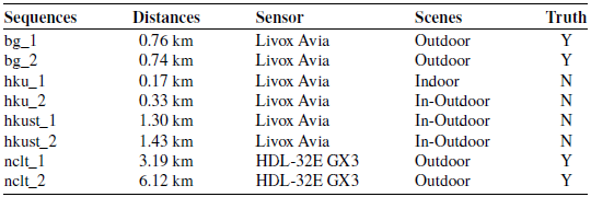
This section presents a series of experiments designed to evaluate the computational efficiency, accuracy, and robustness of the LIO system. These experiments are conducted on a total of 13 datasets, including 8 open datasets and 5 self-collected datasets from a campus environment. All LiDAR frame rates are set to 10 Hz.
The information regarding the open datasets, including types of sensors, distances, and scenes, is summarized in Table II. For instance, the BotanicGarden (bg) dataset [Reference Liu, Fu, Qin, Xu, Xu, Chen, Goossens, Sun, Yu, Liu, Chen, Tao and Zhao31] is collected using a spinning LiDAR, the Livox Avia (
 $70.4^\circ \!\times \! 77.2^\circ$
FoV), operating at 10 Hz, and a 9-axis Xsens MTi-680G IMU sampled at 400 Hz. This dataset features long loop closure paths. The hku dataset and the hkust dataset [Reference Lin and Zhang32] cover both indoor and outdoor scenes collected by a FLIR Blackfiy global shutter camera, a Livox AVIA LiDAR, and a built-in IMU at the Hong Kong University of Science and Technology and Hong Kong University. The nclt [Reference Carlevaris-Bianco, Ushani and Eustice33] dataset contains a Velodyne HDL-32E LiDAR at 10 Hz and a Microstrain MS25 IMU sampled at 50 Hz, featuring long trajectories from the University of Michigan’s North Campus. The open datasets utilized in this study are representative and are used to validate the algorithm’s performance from multiple perspectives.
Details of open datasets.

In addition to the open datasets, we also collected various challenging data on our self-built platform (see Figure 4). The mobile robot experimental platform used in this paper is equipped with an AMD Ryzen 3 3200G CPU. The sensor suite includes a Livox Avia solid-state LiDAR with a non-repetitive horizontal FoV of
 $70.4^\circ$
and a vertical FoV of
 $77.2^\circ$
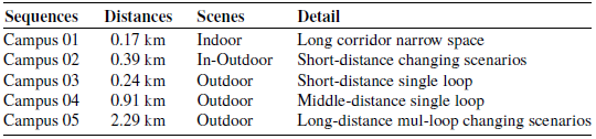
, capable of ideally obtaining 240,000 laser points per second. The IMU integrated within the Avia LiDAR is BMI088 model, a 6-axis sensor comprising a 3-axis accelerometer, and a 3-axis gyroscope, providing data at an output frequency of 200 Hz. All the self-collected campus datasets in this paper are from the South China University of Technology campus, and the detailed information of the multiple campus environments is presented in Table III. Clearly, the campus datasets provide a comprehensive foundation for validating the algorithm.
Details of campus datasets.

Experimental equipment setup for campus datasets.

7.2. Computational efficiency
We evaluate the algorithm’s computational efficiency and accuracy using both open datasets and campus datasets. All experiments were conducted on a comprehensive simulation validation platform equipped with an AMD Ryzen 7 7735H CPU and an NVIDIA 3060 GPU. The same resolution was used for point cloud downsampling in all algorithms.
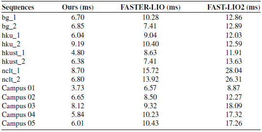
Table IV compares the average computational time per scan (10 Hz) with an average of 1862 effective feature points between our algorithm, FASTER-LIO, and FAST-LIO2. Baseline selection prioritizes methods optimized for solid-state LiDARs (e.g. FAST-LIO2 [Reference Xu, Cai, He, Lin and Zhang16], FASTER-LIO [Reference Bai, Xiao, Chen, Wang, Zhang and Gao18]), which outperform spinning LiDAR-oriented approaches (e.g. LIO-SAM [Reference Shan, Englot, Meyers, Wang, Ratti and Rus25], LOAM [Reference Zhang and Singh22]) in handling irregular scan patterns. Other methods require over 10 ms to process a single frame of scan, while our algorithm consistently operates in less than 10 ms, reducing the average computation time by 24.7–60.1%. Particularly in outdoor datasets such as nclt and Campus 05, where FAST-LIO2 requires 26 ms per scan, our method only needs 6 ms, achieving a reduction in processing time of nearly 75%. The speed of our algorithm is attributed to avoiding pairwise point comparisons and utilizing approximate correspondence matching during the VGICP procedure. The faster convergence is achieved through the use of the Gauss-Newton method.
Next, we evaluate the average processing time for each step, as shown in Figure 5. Our algorithm can save approximately 23.5–66.4% of the processing time for LiDAR measurement and state updating while consuming more time during the downsampling step. That is because our algorithm achieves concurrent processing of covariance calculation and voxelization, so the process of covariance calculation is categorized under the downsampling step in our method.
Average time consumption per scan at 10Hz.

Time consumption in each step compared with advanced methods. (left: Ours, middle: FASTER-LIO, right: FAST-LIO2).

7.3. Accuracy
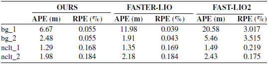
For the sequences that adopt the GPS values as the ground truth: bg_1, bg_2, nclt_1, and nclt_2, we calculate the root mean square error (RMSE) of the absolute pose error (APE) to evaluate the overall trajectories evaluation and the relative pose error (RPE) to assess drift. The error is computed based on the difference between the ground truth trajectory and the algorithm trajectory. As shown in Table V, our algorithm demonstrates superior APE performance compared to other algorithms. Our algorithm exhibits good localization accuracy in both short and long distance datasets, with the exception of the bg_2 dataset, where the localization accuracy is slightly inferior to that of FASTER-LIO. Additionally, the RPE of our algorithm is better than that of FAST-LIO2 and achieves comparable accuracy to FASTER-LIO at a faster processing speed (typically with a relative pose error of 0.05–0.15 m). The marginally higher RPE observed in bg_1 and bg_2 results from environmental factors beyond sensor FoV limitations, specifically dense foliage inducing laser absorption and multi-path reflections. These conditions degrade point cloud integrity, as evidenced by FASTER-LIO’s 11.98 m APE in bg_1. Under such feature-sparse conditions, our method achieves 60.1% faster processing than FAST-LIO2 (Table V), demonstrating significant efficiency gains in geometrically degraded scenarios characteristic of narrow FoV environments.
Trajectory accuracy evaluation using APE and RPE metrics.

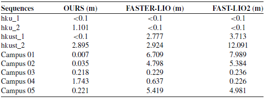
End to end errors.

For the self-collected campus datasets and the partially open datasets that lack ground truth, the localization accuracy was evaluated using end-to-end error. Ignoring fluctuations within 0.1 m, the data in the Table VI indicate that our algorithm maintains the same level as the existing algorithms in terms of accuracy and slightly outperforms the other two algorithms in dynamic scenes. On the Campus 05 trajectory, our odometry achieves an end-to-end drift of 0.221 m without loop closure, demonstrating low inherent drift. The system outputs keyframe poses with associated covariance matrices
 $\hat{\mathbf{P}}_k$
and compressed voxel submaps, ensuring compatibility with back-end optimization frameworks such as GTSAM.
In Campus 04’s long corridors (Figure 7c), solid-state LiDARs’ narrow FoV causes feature degradation, yielding 1.743 m end-to-end error (Table VI). While FASTER-LIO and FAST-LIO2 achieve lower localization errors (0.637 and 0.226 m, respectively), our approach maintains significantly faster processing.
Next, we conducted a trajectory analysis of bg_1, as shown in Figure 6. All three algorithms are able to achieve relatively accurate fitting to the ground truth in the x-axis and y-axis. However, there is a large gap between the position obtained by the algorithms and the ground truth in the z-axis, primarily due to insufficient sensor observations. Specifically, our algorithm achieves an average APE of 5.86 m in the z-axis, compared to an average APE of 12.14 m for the other algorithms. As the algorithms continue to process data, the localization errors gradually increase, but our algorithm exhibits a smaller error. That is because our algorithm effectively mitigates the deviations of localization caused by a lack of feature points.
Mapping result of ground-true and different LIO methods in bg_1. (a) 3D trajectory diagram. (b) Localization error of three axis.

The mapping results for the Campus dataset are shown in Figure 7. In Campus 01, an area of
 $76\,{\text{m}} \!\times \! 17\,{\text{m}}$
is mapped accurately, with no large angular offset throughout the operation (localization drift less than 0.7% over a 170-m trajectory). Experiment conducted in Campus 02 demonstrates that our algorithm has satisfactory transition capabilities at the boundary between indoor and outdoor areas (4.3% drift in 396 m trajectory). In Campus 03, 04, and 05, motion trajectories of the mobile robot are relatively simple, resulting in nearly identical trajectories generated by three algorithms.
Mapping results of different LIO packages in Campus dataset. Blue: OURS, green: FASTER-LIO, red: FAST-LIO2. (a) Campus 01. (b) Campus 02. (c) Campus 05. The trajectories of Campus 03 and Campus 04 generated by three algorithms are too similar to be displayed separately.

7.4. Robustness
The robustness of the proposed method was evaluated using the Campus 01 dataset. This dataset was collected by a mobile robot navigating indoors on campus, traversing narrow corridors, negotiating tight right-angle corners (creating limited-FoV scenarios), folding back at the end, and finally returning to the initial pose. The Campus 01 dataset presents three significant challenges for LIO: (1) long straight corridors with sparse features, susceptible to heading drift; (2) severe FoV restrictions during sharp turns, causing sudden feature loss; and (3) temporary occlusions or pedestrian crossings, introducing dynamic object interference to point cloud matching.
Our method is compared against FAST-LIO2 and FASTER-LIO algorithms. As shown in Figure 7(a), the trajectories of baseline methods exhibit pronounced divergence from the ground truth path during right-angle turns, while our algorithm maintains precise path following. Crucially, these turns create challenging limited-FoV scenarios where baseline methods accumulate unrecoverable drift due to feature loss. Detailed pose analysis in Figure 8 reveals that baseline methods develop substantial y-axis drift and yaw deviations during turning periods, directly attributable to FoV limitations. In contrast, our method maintains stable pose estimation throughout the trajectory.
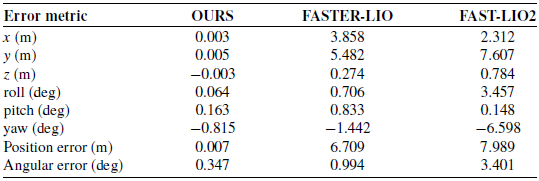
Quantitative results in Table VII confirm these observations: baseline methods exhibit considerable terminal position errors (FASTER-LIO: 6.709 m, FAST-LIO2: 7.989 m) and angular deviations (FAST-LIO2 yaw: −6.598
 $^\circ$
), while our method achieves minimal error (position: 0.007 m, angular: 0.347
 $^\circ$
). This significant difference stems from baseline methods’ inability to handle FoV restrictions during sharp turns, where they lose critical features. These results explicitly demonstrate our method’s robustness in limited-FoV scenarios, maintaining accuracy through adaptive keyframe management and motion-compensated feature association where baseline algorithms fail.
8. Conclusion
This paper proposed a computationally efficient and accurate LIO framework. First, we designed a novel SVMs to reduce the consumption of computation; subsequently, we developed a GICP algorithm based on sparse voxels, which outperforms other point cloud registration methods in terms of processing speed; finally, we analyzed the residuals and covariance of the IMU and LiDAR, and achieved sensor data fusion through the Gauss-Newton method. The algorithm was validated on both open datasets and campus datasets, and the experimental results demonstrate that our algorithm maintains the localization accuracy and robustness of the LIO while significantly improving computational efficiency.
Pose estimation errors on Campus 01 dataset.

Pose analysis on Campus 01 dataset. (a) Position errors along three axes (b) Euler angle variations.

Author contributions
All authors contributed to the study conception and design. Zi Ding conducted data gathering and wrote the article. Pengfei Lyu performed statistical analyses. Wei Xie and Langwen Zhang provided critical revisions to the manuscript.
Funding statement
This work was supported by the Guangdong Basic and Applied Basic Research Foundation under Grant 2025A515010413 and Grant 2023A1515240070.
Competing interests
The authors declare that no conflicts of interest exist.
Ethical approval
Not applicable.