Introduction
The Antarctic continent is often cited as being the highest, driest, windiest, and generally one of the most hostile environments on Earth. Despite great improvements in satellite and model data products and reanalysis datasets in recent years, a considerable proportion of study of the Antarctic atmosphere continues to be dependent on data collected in situ by automatic weather stations (AWSs).
The importance of this form of data in Antarctica is illustrated by the wealth of studies that have incorporated such records into their analyses since the large-scale introduction of AWS units into the Antarctic in the early 1980s. Early results from AWS studies are summarized by Stearns & Wendler (Reference Stearns and Wendler1988). Data are particularly useful in analysing local and mesoscale meteorological effects and have been used to study the temperature and wind characteristics of many regions of the continent. The Ross Ice Shelf air stream and associated Transantarctic Mountains barrier flow (O'Connor et al. Reference O'Connor, Bromwich and Carrasco1994, Seefeldt et al. Reference Seefeldt, Cassano and Parish2007, Steinhoff et al. Reference Steinhoff, Chaudhuri and Bromwich2009) have been particularly well-studied due to the development of a network of AWS sites on the Ross Ice Shelf over the course of several decades. Around Ross Island, AWS data have been used to predict strong winds that may prevent aircraft activity (Holmes et al. Reference Holmes, Stearns, Weidner and Keller2000) and aided in the study of the anomalously calm area of Windless Bight (O'Connor & Bromwich Reference O'Connor and Bromwich1988). Within the Transantarctic Mountains data have been used to study katabatic and anabatic flows (Zawar-Reza et al. Reference Zawar-Reza, George, Storey and Lawson2010). In the McMurdo Dry Valleys, katabatic and föhn activity have been investigated (Doran et al. Reference Doran, McKay, Clow, Dana, Fountain, Nylen and Lyons2002, Nylen et al. Reference Nylen, Fountain and Doran2004). Data from the high plateau of East Antarctica have also been analysed (Zhou et al. Reference Zhou2009), as have data from the area around Terra Nova Bay (Cogliani et al. Reference Cogliani, Abbate and Racalbuto1996). These articles represent only a small cross-section of published research dealing with Antarctic AWS data. It is clear that a large sum of knowledge on Antarctic meteorology has been acquired through the use of such devices. Furthermore, AWS data have also been employed to determine and validate long-term temperature trends and changes in circulation. Information of this type is extremely important given that, in contrast to the majority of the Earth's surface, the spatial temperature trends of Antarctica are neither fully known nor fully understood. Single long-running AWS sites can furnish data on long-term trends in a local area, such as at Fossil Bluff on the Antarctic Peninsula (Harangozo et al. Reference Harangozo, Colwell and King1997) and three West Antarctic stations investigated by Shuman & Stearns (Reference Shuman and Stearns2001). Data have also been used in large-scale and continent-wide assessments (Jacka et al. Reference Jacka, Budd and Holder2004, Steig et al. Reference Steig, Schneider, Rutherford, Mann, Comiso and Shindell2009). Studies that have utilized gridded reanalyses datasets, such as the NCEP/NCAR or ERA40, are also dependent on in situ data for both input and verification (e.g. Yu et al. Reference Yu, Zhang, Zhou, Zhong, Lenschow, Hsu, Wu and Sun2010).
While improvements have been made in the AWS network distribution (Lazzara et al. Reference Lazzara, Weidner, Keller, Thom and Cassano2012), Antarctic AWSs are still relatively thinly spread, particularly in the continental interior. Furthermore, as a result of the extreme weather of the continent and the difficulties and cost in transport and logistics, it is inevitable that AWS systems occasionally fail, leading to gaps in an already sparse dataset. Quality control can become problematic with particularly remote stations, as there exist no reference data to compare suspect records. Research into localized effects has also suffered because of the sparse nature of AWS sites and coarseness of model grids, particularly in the complex coastal margins.
Thus, the problems with current AWS design and spread are twofold: firstly, there is a lack of redundancy within the AWS network, secondly, small-scale meteorological and climate effects are ill-understood, due to a paucity of data at kilometre scales. Over the summer Antarctic field season of 2011/12, a team from the University of Canterbury carried out tests of a novel meteorological monitoring system called SNOW-WEB. The system consists of a network of simple, cost-effective weather stations that can be deployed efficiently in snow- and ice-covered conditions. The system is equipped with GPS technology for accurate positioning and time-keeping, and the potential for measuring ice shelf movement. Individual stations carry onboard wireless transceivers, enabling them to transfer data in real-time and be controlled remotely from manned bases in the region or via an internet interface. The system adds redundancy to data collection as a large number of stations can be deployed in a small area, ensuring data collection continues if one or more stations were to fail due to high wind events or other malfunctions. SNOW-WEB provides a large volume of spatially detailed data over the deployment area that would not be captured by a single AWS. Finally, the distributed nature of the system can aid with the validation of gridded datasets.
Field testing has confirmed that the concept of wireless data transfer over tens of kilometres in Antarctica is viable and has provided a large amount of meteorological data for study. This paper reports on the development of the system and our findings thus far. The following section gives a description of the SNOW-WEB network. This is followed by a report on the deployment and withdrawal of the equipment during the 2011/12 field season and the functioning of the network during its deployment. We perform a validation of the data collected by the network using pre-established weather station data from the observation region. A comparison is performed with output from the Antarctic Mesoscale Prediction System (AMPS). We also present a case study that highlights the advantages of SNOW-WEB data, and finally offer a summary and details on planned future development of the network.
SNOW-WEB description
SNOW-WEB is a distributed system of environmental monitoring sensors designed and constructed by the Atmospheric Group, Department of Physics & Astronomy, at the University of Canterbury, New Zealand. The system is specifically designed for use in Antarctica. It consists of a series of low-cost and low-power weather stations that can be deployed over a large area, in order to provide robustness and redundancy to weather and climate monitoring and to facilitate high-resolution meteorological studies. The system is unique in Antarctica in that each node is equipped with a wireless transceiver, enabling it to communicate remotely with its neighbours via the mesh-networking ZigBee protocol. Data can then be routed back to a coordinating computer at a manned station in the region. The wireless communication is handled by Digi XBee-Pro Series 2 wireless transceivers, operating at 2.4 GHz. The transceivers are pre-installed with advanced wireless mesh-networking protocols for the purposes of routing data. Each transceiver has a unique serial number, which can be used to address packets specifically to that device. This unique address is also used to identify nodes from their transmissions by logging software. One major limitation of remote data transfer at this frequency is that line-of-sight is required between nodes for transmissions to succeed. This is a particularly pressing issue in Antarctica, where surface wind flows tend to be tied to the underlying terrain, and thus line-of-sight problems are most likely to occur in areas where the wind field is interesting due to complex topography. By strategically placing nodes and using high-gain antennae these areas can still be sampled. Whilst the SNOW-WEB deployment range was dictated mostly by logistical considerations, terrain can limit the range of networks that rely solely on wireless communication.
The SNOW-WEB system incorporates three types of node, with important distinctions between their operation. What follows is a description of the hardware and workings of each flavour of node.
Coordinator node
The coordinator node is a transceiver programmed with firmware that takes control of the network, constructs a table of networked nodes, and handles packet routing. For the purposes of the SNOW-WEB network, all data packets containing meteorological and GPS positioning information are routed towards the coordinator, which is connected to a computer via Universal Serial Bus (USB). The computer is programmed with data-logging software, such that users can download data and view it in real-time. The software also handles user remote control of the network.
During the 2011/12 field season, the coordinator node of the SNOW-WEB network was located at Scott Base, Ross Island. A communications mast provided elevation and hence better line-of-sight transmissions for the attached 1.5 m passive isotropic antenna to increase the range of broadcast and transmission.
Primary node
Within the ZigBee mesh-network framework, primary nodes are designated as ‘routers’. This means that they must be powered all the time, as they are required to route transmissions from distant nodes towards the coordinator. They act as the spine of the network as all information proceeds through them.
Primary nodes are controlled by an AVR ATmega64 microcontroller which is used for data logging and initial processing. They are equipped with a temperature and relative humidity (RH) sensor (Sensiron SHT75), and wind speed (NRG #40H) and direction (NRG #200P) measuring devices. They also include a GPS module (Navman Jupiter 130) for ice shelf and glacier movement studies. The GPS also provides accurate time information for synchronization across the network, and its one-second output is used as a timer for processes such as data collection and transmission. A Secure Digital (SD) memory card provides ample onboard data storage for the nodes, which is particularly important if the network fails.
The default time resolution of the primary node is a 30 second meteorological data collection interval, accompanied by the collection of GPS data at two minute intervals. However, wireless connectivity allows the user to change the default interval of data collection from 30 seconds to ten seconds, if an interesting meteorological event is evident. Ultimately, future designs will have logging software loaded onto the coordinator node that will be able to intelligently ascertain significant changes in weather conditions and alter the time resolution accordingly. Wireless connectivity also allows the user to manually reset the network or an individual node via the coordinator, if that node has failed. Individual nodes can also be queried for specific data, such as remaining power or memory capacity.
Automatic communications between the primary and coordinator nodes are straightforward. A standard format of data string is defined, and each time the node records either meteorological or GPS data it is forwarded on to the coordinator node to be recorded on the computer at the base station.
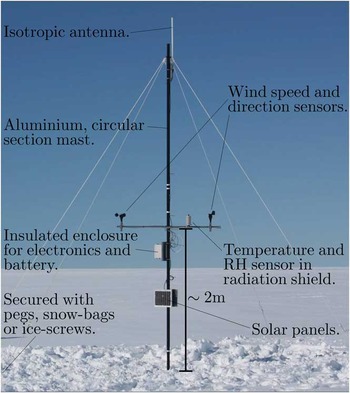
Figure 1 shows a photograph of the mechanical design of the primary node, consisting of a series of 2.2 m circular-section anodized aluminium poles, which interlock to form a mast from 2–6 m high, in 2 m intervals. The mast's varying height allows the user to overcome problems of line-of-sight due to uneven terrain. The mast is anchored at the surface by a wooden base, attached with an articulated joint to aid in erection. The base is dug into the snow or ice for support. Four guy ropes are attached to the top of the mast and secured at ground level by snowbags, pegs or ice-screws, depending on the terrain. At 2 m above snow-level, a boom is attached, on which are mounted the atmospheric sensors, with the temperature and relative humidity sensor contained in a radiation shield. Cables from these lead to a well-insulated box below the boom, which houses the data logger and battery. A 1 m passive isotropic antenna is mounted at the top of the mast. Primary nodes are powered by a single 12 V sealed lead-acid battery, and charged by two 5 W solar panels, which are attached to the mast below the electronics box, perpendicular to the ground for maximum incident radiation and minimum snow accumulation.
Photograph of primary node mechanical design.

Secondary node
Secondary nodes are scaled down primary nodes, designed to increase the spatial extent of the network whilst maintaining low power consumption. They are controlled by a much lower power microprocessor, the AVR ATtiny2313a. This limits their functionality to collecting temperature and relative humidity data, and transmitting to their parent node. Secondary nodes are designated as ‘end device’ nodes in the ZigBee scheme. This means that they do not route data, they merely communicate with a parent node, a router or coordinator that is also part of the network. This allows the secondary nodes to turn their transceivers to sleep for the majority of the time.
The lessened processing power of the secondary node and the lack of GPS or a real-time clock to provide time information dictates that the secondary must send its raw data to its parent primary, which then processes and saves the data and forwards it to the coordinator. The lack of processing power also means that the secondary node cannot be controlled via wireless connections, it simply sleeps, wakes up, takes a reading, forwards the reading to the parent node, and then returns to sleep. This allows the secondary node to have very low power consumption.
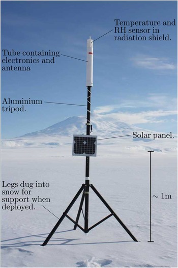
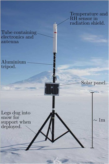
The mechanical design of the secondary node is shown in Fig. 2. It consists of an aluminium tripod, on which sits an insulated cylindrical tube, which houses the electronics and a c. 20 cm passive isotropic antenna. On top of the tube is a radiation shield, containing the temperature and relative humidity sensor (SHT75). For deployment, the three legs of the tripod are dug into the snow or ice, and covered. The upright pole of the tripod is extendable, such that the sensors can be accurately positioned at 2 m above snow level. The tripod design allows very rapid deployment of the secondary nodes, which is a significant advantage in the Antarctic environment. Secondary nodes are powered by a 3.7 V lithium-ion battery pack, and a single 5 W solar panel, mounted on the tripod, perpendicular to the ground.
Photograph of secondary node mechanical design.
Sensors and uncertainties
The temperature and relative humidity sensor used on both the primary and secondary nodes is the Sensiron SHT75. The manufacturer specified uncertainty on this device is ± 0.5°C at 0°C, which increases linearly to ± 1°C at -20°C. The average summertime temperature in the SNOW-WEB testing area is c. -5°C, hence the general uncertainty of the sensor over the observational period will be in the region of ± 0.6°C. For relative humidity the uncertainty is ± 2% within the range of 10–90%.
Wind speed data are collected by a vertical axis cup-type anemometer, the NRG #40H. An electrical pulse is induced at a specific point in each rotation of the device. The microprocessor times the interval between successive pulses to determine the angular frequency. A calculation is then performed to convert this frequency into a wind speed based on the physical properties of the anemometer. The maximum counting period of the microprocessor limits the minimum wind speed that the device can record to 0.6 m s-1, hence all wind speed values below this are recorded as 0 m s-1. The highest wind speed that can be handled by the sensor is given as 96 m s-1, which is vastly higher than any wind speed encountered in Antarctica during the summer months. Measurement uncertainty is ± 0.14 m s-1 at 10 m s-1, but probably slightly higher away from this magnitude as the linear transformation from frequency to wind speed becomes less accurate. We consider a conservative estimate of the uncertainty on the wind speed to be ± 0.3 m s-1.
Wind direction information is recorded via an NRG #200P wind vane. The device measures direction via a potentiometer connected directly to the vane. The potential is communicated to the microprocessor via an analogue to digital converter. The stated linearity of the potentiometer is 1%, thus a conservative estimate of the uncertainty of the device is ± 3°.
Field report
Deployment environment
For approximately two months of the summer field season of 2011/12, SNOW-WEB was deployed on, and in the vicinity of, Ross Island, Antarctica. Ross Island is a mountainous, predominantly snow-covered island at the north-western edge of the Ross Ice Shelf. The topography of the island is dominated by a chain of three mountains, Erebus, Terra Nova, and Terror, which proceed from west–east. At the south-east of Mount Erebus descends the Hut Point Peninsula, at the tip of which lie the primary American and New Zealand Antarctic research bases, McMurdo Station (77°51′S, 166°40′E) and Scott Base (77°51′S, 166°45′E), respectively. To the west of the island lies McMurdo Sound, and beyond this the Transantarctic Mountains and McMurdo Dry Valleys. To the north is the Ross Sea. To the east and south is the Ross Ice Shelf, the largest of the Antarctic floating ice masses. The shelf consists of almost flat, floating ice that can be up to several hundred metres thick. Two ice runways, Pegasus and William's Field are located to the south-west and east of the Hut Point Peninsula, respectively. To the immediate south of the island is the wide bay, Windless Bight, bounded by the Hut Point Peninsula to the west and Cape MacKay to the east. Further south are White Island and Black Island, and the barrier of Minna Bluff.
Ross Island is located at the northern end of the Ross Ice Shelf air stream (RAS), which is characterized by a strong south and south-easterly flow. The RAS is a semi-permanent feature of the Ross Ice Shelf, which displays strong low-level flow parallel to the Transantarctic Mountains. It is fed by katabatic drainage at the Siple Coast at the south-east border of the Ross Ice Shelf and glaciers within the Transantarctic Mountains to the south. Investigation of the RAS has been performed by Parish et al. (Reference Parish, Cassano and Seefeldt2006), Seefeldt & Cassano (Reference Seefeldt and Cassano2008) and Seefeldt & Cassano (Reference Seefeldt and Cassano2012), using output from the AMPS model. Dominant wind regimes in the region have also been studied by Seefeldt et al. (Reference Seefeldt, Cassano and Parish2007) using AWS data. A climatology of the Ross Island region was given by Monaghan et al. (Reference Monaghan, Bromwich, Powers and Manning2005) using archived AMPS output.
The action of the southerly wind as it encounters the high and steep slopes of Ross Island has also been the focus of study. Detailed analyses of the wind field of the area including theoretical and model studies have been carried out by O'Connor & Bromwich (Reference O'Connor and Bromwich1988) and Seefeldt et al. (Reference Seefeldt, Tripoli and Stearns2003). They found that southerly wind flow often does not have sufficient energy to overcome the elevated terrain of Ross Island, and thus cold air is piled into Windless Bight, generating a pressure gradient that causes calm conditions within the bay, and the turning of the wind to the north-east in a typical barrier flow regime (Schwerdtfeger Reference Schwerdtfeger1984). It is this effect that causes the prevailing wind at Scott Base to be from the north-east.
Ross Island is then clearly interesting in a meteorological sense and, given its vicinity to research bases, logistically ideal for the testing of new AWS technology. Validation and understanding of meteorological data is also aided in that the region around Ross Island has a very high density of AWS sites and 12-hourly radiosonde launches from McMurdo Station. The area is also serviced by the the finest AMPS grid of 1.67 km and hourly time resolution.
Deployment
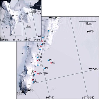
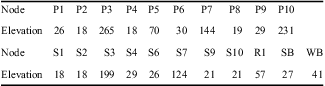
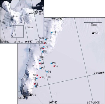
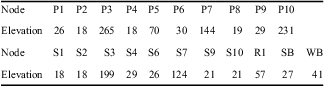
SNOW-WEB was deployed from Scott Base, with a field camp at ‘Room With A View’ (unofficial name), a snow-covered outcrop at the top of the Hut Point Peninsula between Scott Base and Mount Erebus. The light-weight design of the nodes allowed for ski-mobile and Hägglund to provide adequate transport for the deployment. A four person team deployed ten primary nodes and eight secondary nodes along the Hut Point Peninsula and across the ice shelf to the south during early December 2011. An experienced team could erect a primary node in less than one hour and a secondary in 15 minutes. Node communication was tested at the time to ensure adequate line-of-sight transmission for a robust network. Careful planning also ensured that several pathways for data transfer were established from the farthest nodes to guard against data loss due to node failures. The coordinating node was located at Scott Base and the farthest node was located c. 25 km away at ‘Room With a View’. Both the coordinating node and the farthest node were equipped with larger (c. 1.5 m) isotropic antennae for enhanced data transfer range. A line of nodes was then populated to the west and south of ‘Room With a View’, descending the Hut Point Peninsula onto the ice shelf towards Scott Base, with the closest node (P4) stationed c. 3 km from the base. Several nodes were also deployed on the ice shelf to the south, along the flagged route to Windless Bight. This ensured a second path for data from the farthest nodes and also allowed an elevation profile to be sampled. Figure 3 shows a map of the resulting network layout. Altitudes of nodes above mean sea level are given in Table I. Final changes to the network firmware were made on 10 December 2011.
SNOW-WEB distribution in vicinity of Hut Point Peninsula for 2011/12 field season. Primary nodes are designated with a ‘P’ and blue dot. Secondary nodes are shown by red dots and an ‘S’. Locations of McMurdo Station (McM), Scott Base (SB) and the Windless Bight (WB) automatic weather station site are shown in black. R1 (grey dot) is a repeater deployed to further network connectivity. P3 is situated at ‘Room With A View’. Inset shows greater Ross Island area. Satellite imagery is provided by LandSat Image Mosaic of Antarctica (LIMA).
SNOW-WEB node elevation data (in metres), as well as meteorological stations used in subsequent analysis. Elevation data is sourced from the Radarsat Antarctic Mapping Project (RAMPS) (Liu et al. Reference Liu, Jezek, Li and Zhao2001).
SNOW-WEB was left in place for nearly two months of the summer season. During this time, its data logging and transfer routines, electronic and mechanical design, and remote control systems were tested. A second four person team withdrew the network in late January 2012. Nodes were retrieved from 30–31 January, giving a total observational time of 52 days.
Network evaluation
During the observational period, SNOW-WEB nodes transferred a total of 12.2 MBytes of useful data to the coordinating node at Scott Base, and recorded 24.5 MBytes via onboard SD card. Remote control of the network, carried out from Scott Base directly after the deployment and prior to withdrawal times, was demonstrated to be functional. Individual nodes could be polled for data or given commands, and all currently networked nodes could be manipulated from Scott Base. Equipped solar panels provided ample power for the nodes. Sensors and electronics also showed themselves to be robust enough for the summer months, with no physical failures while deployed. The mechanical designs of both the primary and secondary nodes were shown to be adequately hardy, with a few minor changes needed to the primary to aid in efficient erection in the often hostile Antarctic environment. The secondary node design, although in need of some development, was exceptionally quick and easy to deploy, and robust enough for the summer season.
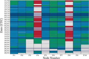
SNOW-WEB successfully transferred meteorological and GPS data from distances of up to 25 km to a manned station via wireless networking. However, an unresolved networking error of the secondary nodes, thought to be a problem with the sleep routine, prevented any significant amount of data being collected from all but two secondary nodes, S9 and S10. Wireless transfer from the primary nodes was far more successful. However, transfer was sometimes erratic and unreliable. In total, accounting for coordinator down-time, 42% of available data was successfully transferred to the coordinator. SD memory card records are more comprehensive, but also included some failures. A diagram illustrating the types of data collected over the experimental period is shown in Fig. 4.
Diagram showing the data collected from each node over the course of SNOW-WEB deployment. Times shown in light and dark blue represent data saved to the onboard Secure Digital (SD) memory. Red represents times when data were recorded via the coordinating node. Green represents times when both methods occurred simultaneously. White represents times when no data were recorded. Dark blue and grey areas show times when the coordinating computer was not operational, and so recording via wireless transfer could not occur.

Figure 4 shows that all primary nodes with the exception of P4 and P8 recorded a significant volume of data to their onboard SD cards. Several failures are evident though, particularly towards the end of the experiment. P3 and P5 for instance, both failed in mid-January due to a firmware overflow associated with corrupted SD memory cards. The overflow caused the primary nodes to continuously reset and cycle power. This resulted in the node leaving and rejoining the network each minute, and hence precluded both SD and wireless records from the affected nodes. As the experiment continued, further nodes were affected by this fault and ceased recording data.
Very little SD memory data was retrieved from P4 or P8. In the case of P4, this was due to a defective SD card reader, although this node did record some data via SD in mid-January. P8 recorded significant data to its SD card, but the data was lost due to a physical failure of the main data chip. Fortunately, each of these nodes transferred a significant volume of data to the coordinating node, which at least in part demonstrates the robustness of the system to physical failures.
Figure 4 shows that P5 collected a significant amount of data. However, upon observation of the data many anomalous points can be identified. Temperatures exceeding 30°C are present, as are wind directions that are regularly out of sync with the rest of the network. Similar recording patterns seen in P5 SD records upon retrieval have led us to believe that data from this node is unreliable due to an error within the microprocessor. The remainder of this paper will disregard P5 data for this reason.
Malfunctions in the logging hardware caused occasional gaps in the wireless transfer record. These gaps are shown by dark blue (for times and nodes where SD data are present) or grey (for times where no data are present) in Fig. 4. Other networking drop-outs are harder to explain. Analysis carried out on the data in search of drop-out cascades, in which one node leaves the network causing others to follow, proved inconclusive. This is possibly due to the fact that several transfer paths were present in the network topography. Thus, a single drop-out might not affect the total transfer to a great degree. Importantly, drop-outs did not appear to be dependent on atmospheric conditions.
A lack of adequate routing throughout the network is another possible explanation for the erratic nature of the data transfer. It was found that if the coordinator gave a network reset command then several, if not all, of the primary nodes would rejoin the network and resume data transfer. It is possible that network traffic proceeded through a small subset of nodes, which became over-loaded and incapable of ferrying signals. As the primary nodes need occasional messages from the coordinator in order to stay on the network, these messages may have been queued, and hence the nodes would leave the network to search for another.
A second possibility is inadequate flow control. Some nodes were found to be forwarding the data of other primary nodes but never transmitting their own. P1 for instance, forwarded much data from more distant nodes in a route analysis exercise. However, Fig. 4 shows that P1 almost never transferred data to the coordinator. Communication of the data from the microprocessor to the transceiver, while the transceiver was busy could have induced this effect.
Despite developmental problems with the SNOW-WEB networking and data collection routines, we consider the summer field season of 2011/12 to be a successful proof of concept demonstration of SNOW-WEB. Data were transferred wirelessly over tens of kilometres for ten nodes and the network primary nodes operated autonomously for the entire 52 day experimental period. A significant volume of data was also recorded. Further work on improvements in the SNOW-WEB mesh-networking scheme is on-going.
Data validation
Subsequent to the withdrawal of the SNOW-WEB network, a significant volume of data was retrieved from the onboard SD memory cards and coordinating computer at Scott Base. Before data can be used in any meteorological analysis it must be validated to ensure its accuracy and reliability. In order to do this, the data must be compared to pre-existing sources of data in the surrounding area. That the area around Ross Island is the busiest region of Antarctica in terms of human activity aids this objective immensely. There exists a relatively dense network of AWS sites in the region. We will employ data from the AWS at Scott Base (SB), which is operated by the National Institute of Water and Atmospheric Research (NIWA), and the AWS at Windless Bight (WB), which is operated by the University of Wisconsin. The locations of both AWS sites are marked in Fig. 3. An in-depth meteorological assessment of the deployment region is beyond the scope of this paper. We will focus on fundamental atmospheric parameters and statistics in order to validate the data such that it can be used for meteorological purposes in the future.
For the purposes of validation, data series are truncated after 44 days. Inspection of Fig. 4 shows that after this time several of the nodes had stopped working. Mean values taken after this time are therefore unrepresentative of the network as a whole. Validation ignores S10, which was located directly beside S9 for the purposes of a separate radiation shield study, and therefore provides no independent data. As stated above, P5 suffered a prolonged malfunction, and so data from this node are removed from further analysis.
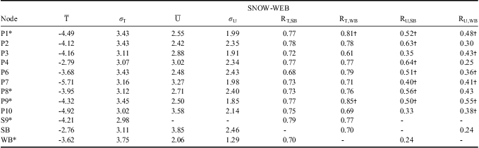
The second to fifth columns of Table II summarize the mean and standard deviations of temperature and wind so that simple comparisons can be made between SNOW-WEB nodes and SB and WB. Scalar wind speed is used in the analysis rather than resolving into zonal and meridional components. Complex topography is known to turn wind in the region such that a comparison of zonal and meridional wind speeds over spatially distant stations makes little sense. We use scalar wind speed to represent the overall wind field of the area.
Statistics for SNOW-WEB. T represents temperature, while U is the scalar wind speed. R is the canonical correlation coefficient. Units for temperature are °C, and wind speed m s-1. SB = Scott Base, WB = Windless Bight.
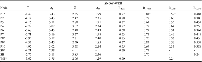
†denotes that a correlation is significantly different from that of SB-WB at the 99% level.
*denotes that the node is situated on the ice shelf towards WB.
Table II shows that the majority of SNOW-WEB nodes have temperature means and standard deviations that are very similar to the established meteorological stations. The coldest nodes are those on the slopes leading up to ‘Room With a View’ (P7 & P10), while the warmest are those close to the base of the peninsula (P4, P6 & P8). The average temperatures at all nodes are colder than that at SB. This is probably due to the ground conditions at the AWS. Scott Base is situated on volcanic rock, which has a significantly lower albedo than the snow-covered ice shelf and peninsula on which SNOW-WEB and WB are located. This may also reduce the amplitude of the diurnal cycle of SB, as it stays warmer for longer during the night. Node temperatures are slightly colder than that at WB.
P4 shows a particularly warm mean temperature, while P7 is particularly cold. It is thought that extremely localized effects may alter the climatology at these stations. P4 is particularly susceptible to the north-westerly wind (see Fig. 5a), which may cause warming in this area. P7 was situated approximately halfway up the slope towards ‘Room With a View’, and was subject to strong down-slope winds and reduced incident radiation due to the slopes to the north, compared to nodes at the top of the ridge. The diurnal variation of temperature of P7 shows that it is as cold at night as nodes on the ice shelf, but not as warm during the day, while ridge-top nodes are warmer at night. This reduces the overall mean at P7 relative to the rest of the network. It is possible that a small calibration bias exists between temperature sensors, although it did not appear in calibration experiments upon the retrieval of the nodes. Temperature standard deviations are comparable across the network and AWS sites.
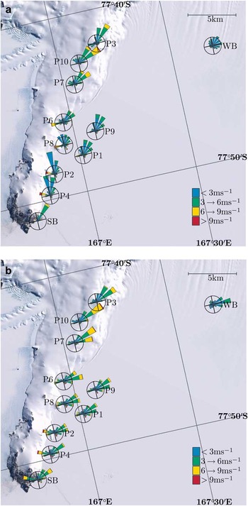
Wind roses for SNOW-WEB, Scott Base (SB) and Windless Bight (WB) data from in situ records and interpolated Antarctic Mesoscale Prediction System (iAMPS) records. Roses represent the 16 cardinal compass points. The distance spanned by petals from the centre represents the frequency of wind from that direction. Coloured sections of each petal represent frequency of wind speeds from that direction. The circle surrounding each rose shows the point of 10% occurrence, except at SB in a., where it represents 20%. Roses are rotated such that compass points are aligned with the map projection. Frequencies are calculated based on the number of available observations. a. SNOW-WEB, and b. iAMPS.

Mean wind speeds are highest at elevated stations, although SB shows the largest speeds in the region. Convergence is observed towards this point in wind roses in Fig. 5a. Calmer conditions are observed at the base of the peninsula and the ice shelf. WB shows the lowest wind speeds. That the speeds measured by SNOW-WEB nodes have magnitudes between those at SB and WB follows expectations and is encouraging in terms of validation. Wind standard deviations are more variable than those for temperature, and appear to scale with increasing wind speed.
Table II also shows canonical correlation coefficients of temperature between SNOW-WEB nodes and SB and WB AWS sites. The correlation between SB and WB is shown for reference and entries that are significantly different from this value at the 99% level are marked. Nodes have consistently high correlations (> 0.7) with both weather stations, which are not significantly different to the correlation between SB and WB. Nodes on the ice shelf show slightly higher correlations with WB than SB. These nodes are marked with an asterisk in the table. For temperature, P1 and P9 have the only correlations which are significantly different from the SB-WB correlation. High correlations of P1 and P9 with WB are probably a reflection of the respective ground conditions and reduced topographical influence further from the peninsula. Nodes at higher altitudes (P3, P7 & P10) show slightly higher correlations with SB, but they are not significantly different from the SB-WB correlation. The correlations of relative humidity (not shown) are of the same order as temperature. The high magnitudes of the correlations further suggest the validity of the SNOW-WEB network data.
Wind correlations with SB are lower than those for temperature and range from c. 0.35 at elevated nodes to 0.63 at P4, the closest node to SB. All nodes except P3 and P10 have significantly higher correlations with SB than the SB-WB correlation, which is rather low. Correlations between the nodes and WB are also reduced. All nodes have significantly higher correlations with WB than SB, except those nodes closest to SB and the base of the peninsula (P2, P4 & P8). Given the well-known influence of topography on modifying wind fields over relatively small distances, it is not surprising that the wind correlations are lower compared to the temperature. The fact that those nodes close to SB show higher correlations is encouraging in terms of data validation. Differences across the network are probably due to underlying differences in the wind field rather than any fault of the SNOW-WEB network. All correlations are significant at the 99% level, except the wind speed correlation of P4 with WB, which is rather low, although still larger than the SB-WB value.
For the purposes of a qualitative assessment of the wind direction and distribution, a wind rose map of the region is displayed in Fig. 5a. The wind rose map shows that the mean wind field of SNOW-WEB data and pre-existing weather data is qualitatively very similar. The direction is modified somewhat by the topography of the region, and hence varies across the station records. However, as mentioned in Seefeldt et al. (Reference Seefeldt, Tripoli and Stearns2003), the dominant wind is light and from the north-east at all stations. The strong southerlies also mentioned in the article do not occur very frequently within the SNOW-WEB dataset, which is probably a product of the season. Strong RAS events that would cause such flows are far more prevalent in the winter and spring (Seefeldt & Cassano Reference Seefeldt and Cassano2008). A secondary peak is seen from the north-west, which is observed even at ridge-top nodes, suggesting that it originates from the sea on the northern side of the peninsula. This peak is confirmed at SB. The distribution is rather different at WB, with eponymously calm conditions. The wind is directed from the north and east predominantly, with occasional north-west and south-easterly components.
AMPS intercomparison
We now examine the SNOW-WEB observations relative to output from archived AMPS forecasts. The generation of AMPS running during the SNOW-WEB deployment period is based on the Polar Weather Research and Forecast (WRF) model. It is initiated with a first-estimate informed by local weather data including AWS and radiosonde records. A description of the working of AMPS and the modifications to WRF to fit the high latitude ice-covered environment is given in Powers et al. (Reference Powers, Monaghan, Cayette, Bromwich, Kuo and Manning2003), Powers (Reference Powers2007) and Hines & Bromwich (Reference Hines and Bromwich2008). The AMPS has been employed in the study of the lower Antarctic atmosphere, particularly in the region around Ross Island and the greater Ross Ice Shelf (Parish et al. Reference Parish, Cassano and Seefeldt2006, Powers Reference Powers2007, Seefeldt & Cassano Reference Seefeldt and Cassano2008, Reference Seefeldt and Cassano2012), where it has identified key circulation features of the area. As a well-established predictive model, we use AMPS to perform an intercomparison with the novel SNOW-WEB data, which serves to validate both data sources and demonstrate the usefulness of SNOW-WEB data. Records from SB and WB are included in the analysis in order to provide a further point of reference. All times in this section are given in UTC, which is thirteen hours behind local time at Ross Island in the summer months.
The highest resolution AMPS sector exists over Ross Island. It is comprised of a 1.67 km polar stereographic grid and proceeds at hourly time steps. Forecasts are performed every 12 hours at 00h00 and 12h00. Following Seefeldt & Cassano (Reference Seefeldt and Cassano2008), we allow a 12 hour spin up for the initial conditions to adjust to the model grid, meaning that the output used is that from 12–23 hours after the forecast initiation. As such, output representing the times 00h00–11h00 on 10 December will be extracted from the 12h00 forecast on 9 December. Output for 12h00–23h00 on 10 December is taken from the forecast of 00h00 on 10 December. At times when the output is missing from a particular forecast we use output from the previous forecast. For example, if 12–23 hour forecast time output is missing from the 00h00 forecast on 10 December then the 24–35 forecast hour output from the 12h00 9 December forecast is used in its place. Using this method we are able to compile an uninterrupted time series from 10 December 2011–31 January 2012.
We use the model air temperature given at an elevation of two metres above ground level. Zonal and meridional winds are logarithmically interpolated to the surface from the two closest pressure levels. AMPS output is interpolated to the locations of the ten SNOW-WEB nodes and the two AWS sites used in the earlier comparison. Interpolation is performed from the four closest grid cells to each weather station. An average is calculated which is weighted by the reciprocal of the distance between the node and the centre of the grid cell, such that the closest cell has the highest weight. This form of interpolation is known to reduce the variance of the resulting interpolated dataset. To counteract this, the interpolated model values are scaled by a factor of  $$--><$>\overline{{{{{\rm{\sigma }}}_{AMPS}}}}/{{{\rm{\sigma }}}_{inter{{p}^} }}}} $$$
, where
 $$--><$>\overline{{{{{\rm{\sigma }}}_{AMPS}}}} $$$
is the mean standard deviation of the four chosen AMPS grid cells, and
 $$--><$>{{{\rm{\sigma }}}_{interp}} $$$
is the standard deviation of the interpolated output. We will refer to the AMPS output interpolated to the spatial positions of SNOW-WEB and AWS sites as iAMPS.
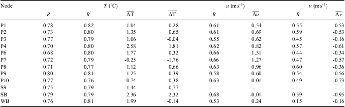
Table III shows statistical relationships between iAMPS values and SNOW-WEB data. We use two statistical metrics to measure the correspondence between SNOW-WEB and iAMPS. The first is the canonical correlation coefficient. The second is the mean bias, which is calculated by taking the difference in records between SNOW-WEB and iAMPS and averaging over all records. Biases are calculated as SNOW-WEB data minus iAMPS, and thus a positive bias indicates that SNOW-WEB averages are higher than iAMPS. Relationships for AWS sites are included for reference.
Computed values of correlation (R) and bias ( $$--><$> \overline{{\rDelta x}} $$$
) between SNOW-WEB node data (including Scott Base (SB) and Windless Bight (WB)) and iAMPS. u (v) is the zonal (meridional) wind speed. Prime values of correlation and bias are calculated from a subset of records that occur concurrently with scalar wind speeds above 4 m s-1.
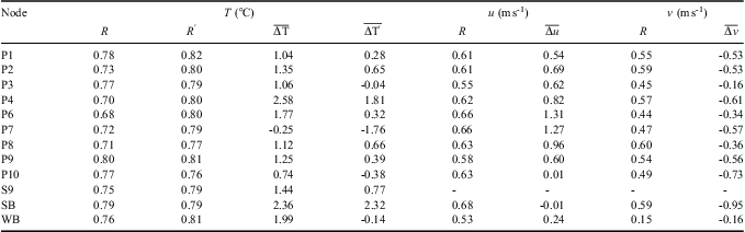
For temperature, we see a very high degree of correlation between iAMPS and SNOW-WEB. All correlations are above 0.7 and statistically significant at the 99% level. Biases range between +1°C and +2°C. Stations highlighted as differing from the norm in the previous section show untypical biases, although the magnitudes of their correlations are comparable to the rest of the network. The bias of P4 is larger than the remainder of the in situ data. P7 shows a slight negative bias. These correspond to results from the previous section, which showed that P4 had an unusually high mean temperature and P7 unusually low.
Complications often arise when measuring temperature in the Antarctic environment because of the high albedo of the ice- or snow-covered surface. Semiconductor-based temperature sensors require thermal equilibrium with the surrounding air to measure temperature accurately. High levels of incident radiation due to the reflectivity of the surface can cause direct heating of radiation shields, which is compounded at low wind speeds due to stagnant air trapped inside. The temperature sensor will then record a temperature that is positively biased compared to the air outside of the shield. Composite days of temperature biases between SNOW-WEB and iAMPS (not shown) reveal more highly positive biases during the early afternoon at all SNOW-WEB nodes and at WB, suggesting that this effect may impact on the general mean. With this effect in mind, we recalculate the correlation and bias between SNOW-WEB and iAMPS using only those records which are concurrent with SNOW-WEB scalar wind speeds > 4 m s-1. The results are shown in Table III as primed variants of the original computed values. Correlations generally increase slightly compared to the original values, although the increases are not statistically significant. The reduction in the bias is large. Biases are reduced to less than 1°C in most cases and at P3, P10 and WB become slightly negative. The bias at P4 is still higher than the remainder of the network, although lower than the original value. All changes in bias (except those of SB and P8) are significantly different from zero at the 99% level derived from a two-sided Student's t-test.
These results indicate that direct heating of radiation shields has caused large positive biases within SNOW-WEB temperature data. However, the effect is observed just as strongly at the established weather station at WB. Genthon et al. (Reference Genthon, Six, Favier, Lazzara and Keller2011) have also reported that large biases are observed by weather stations on the Antarctic Plateau during the summertime. As such, times of strong warming in SNOW-WEB data, concurrent with low wind speeds should be interpreted carefully. Only the value of bias at SB is unchanged by calculating over the subset of data, which suggests that the large positive bias at this station is caused by some other mechanism, perhaps because of the ground conditions at this node. Inspection of the albedo of the AMPS grid shows values of 80% in the area surrounding Scott Base, which is representative of snow or ice cover, but not of exposed rock. The higher albedo used in iAMPS calculations may act to decrease the temperature there.
Temperature biases shown in Table III at higher wind speeds fall within the range reported by Hines & Bromwich (Reference Hines and Bromwich2008) (their table 4), for AWS comparison experiments with the Polar WRF on the Greenland ice sheet. Correlations seen in Greenland appear to be slighter higher than those shown here, which may reflect the relative paucity of data for initiating forecasts in Antarctica, rather than problems with the SNOW-WEB dataset.
Table III also shows equivalent statistics for the zonal and meridional wind at each node. Zonal and meridional winds are used in place of the scalar wind speed as SNOW-WEB nodes and interpolated AMPS output represent the same point in space, and as such both the wind speed and direction should be the same. Correlations are reduced compared to temperature, although they are still significant at the 99% level. Correlations computed at SB are similar to those at SNOW-WEB nodes. Correlations at WB are reduced, suggesting that iAMPS does not reproduce the complicated flow in this area.
Wind is a more difficult variable to simulate in general, particularly in regions of complicated topography where it can change rapidly over small distances. Bromwich et al. (Reference Bromwich, Monaghan, Manning and Powers2005) reported correlations in this region of 0.15–0.31 for zonal and 0.05–0.27 for meridional winds for the 3.3 km grid of the previous generation of AMPS running the polar MM5 model. Much larger correlations were computed for AWS sites on the less complex topography of the ice shelf to the east (their fig. 11b & d). The correlations presented here therefore probably represent an improvement in predictive skill of the current AMPS configuration. It should be noted that these results are valid only for the summer season and may not reflect year-round values. However, Bromwich et al. (Reference Bromwich, Monaghan, Manning and Powers2005) reported reduced correlation coefficients at coastal sites in the summertime compared to winter, attributing the cause to an increased land/sea temperature contrast that is not resolved well by the coarser AMPS grids.
Wind biases are generally small between iAMPS values and SNOW-WEB data, with magnitudes < 1 m s-1, except at P6 and P7. Due to the vector nature of the wind, biases must be carefully interpreted. The prevailing wind in the region is from the north-east. When resolved to its zonal component this produces a negative mean value, as the wind travels in the negative x-direction. Thus, the fact that SNOW-WEB nodes show positive biases for zonal wind implies that iAMPS winds have a larger easterly component of the prevailing wind. This is the case across the network and AWS sites, except at P10 and SB where zonal biases are very small. Zonal biases are particularly large and positive at P6 and P7, which are situated at the base of the peninsula and about halfway up the slope, respectively. It is possible that topographic influences not resolved in the AMPS grid modify the wind at these nodes. Negative biases of meridional wind speed imply that iAMPS has a reduced northerly wind component, which is seen at all nodes.
Mean differences between SNOW-WEB and iAMPS winds are perhaps better illustrated by an analogue to the wind rose map shown in Fig. 5a, and as such we include one in Fig. 5b. Qualitative assessment of the two diagrams shows a degree of similarity between SNOW-WEB and iAMPS on a mean basis. However, iAMPS winds are consistently more easterly than SNOW-WEB, particularly at P6 and P7. Directions of peaks from the north-east appear to match rather well, although they are more frequent in iAMPS. That the differences between SNOW-WEB and iAMPS are also observed at SB and WB suggests that discrepancies are due to deficiencies in AMPS rather than SNOW-WEB. Given that the bias of the easterly wind component increases with proximity to the base of the peninsula, we suggest that AMPS underestimates the ability of the peninsula to act as a barrier and turn the wind to the north, possibly as a result of topographical smoothing.
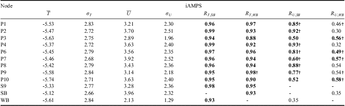
For the purpose of comparing spatial and temporal variability of iAMPS with that of SNOW-WEB, Table IV shows the statistics of mean, standard deviation and correlation for iAMPS. Values are equivalent to those in Table II for SNOW-WEB. Temperature distribution patterns are similar. Scott Base is the warmest interpolated point and P10 the coldest, but temperatures vary more greatly over the region in SNOW-WEB records than in iAMPS. Furthermore, the standard deviation of SNOW-WEB data is larger, suggesting that SNOW-WEB records are more variable than iAMPS. Inspection of iAMPS temperature records shows that they are smoother in general than those of SNOW-WEB (for example, see case study presented below), this is unsurprising given the model resolution. Wind speed distribution is reproduced well. Speeds are higher in general, but show highest values at P7, P10 and SB and lowest at WB, as seen for observations in Table II. iAMPS wind standard deviations match very well with their SNOW-WEB counterparts, suggesting that the time variability is captured well during this period.
Statistics for iAMPS. T represents temperature, while U is the scalar wind speed. R is the canonical correlation coefficient. Units for temperature are °C, and wind speed m s-1. SB = Scott Base, WB = Windless Bight.
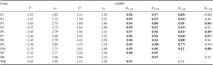
†denotes that a correlation is significantly different from that of SB-WB at the 99% level.
Bold font denotes that correlation is significantly different from the corresponding SNOW-WEB correlation at the 99% level.
For temperature, iAMPS values show significantly higher correlations than SNOW-WEB data with both SB and WB. None of the correlations shown by iAMPS is significantly different from the SB-WB value and all are above 0.9, except P3-WB. This suggests a reduced degree of spatial variability present in iAMPS temperature data. Wind correlations with SB are also increased and significantly different from SNOW-WEB in the iAMPS values, although wind correlations with WB tend to be more similar to those computed from SNOW-WEB data. The lower correlations seen in SNOW-WEB data suggest that local variability is present in the region and that it is under-represented in iAMPS.
In summary, standard statistics presented in this section have shown that the correspondence between SNOW-WEB data and iAMPS output is high, particularly for temperature records. Winds correspond less well, but are qualitatively similar between datasets.
EOF comparison
In order to better compare spatial patterns between SNOW-WEB data and iAMPS output we used an empirical orthogonal function (EOF) analysis. EOF analysis is essentially an eigenvalue decomposition of the covariance matrix of data taken at spatially distinct locations. The technique identifies standing oscillations within the spatial data. The EOF is an eigenvector associated with a particular eigenvalue and contains information on the strength of the oscillation as recorded at any location. The time series of the oscillation can be computed, this is known as the principal component (PC). The proportion of the variance that each PC accounts for within the data can also be calculated.
EOFs and PCs of any data series are scaled to each other rather than to an external value. Thus, in order to reasonably compare the EOFs or PCs of distinct datasets, the datasets themselves must be normalized. We normalize each time series by its standard deviation such that it is dimensionless and has a variance of one. The covariance matrix therefore becomes a correlation matrix. Furthermore, the correlation matrix is sensitive to missing data within the time series. Gaps in the records of SNOW-WEB nodes are filled with data from an average day from that node.
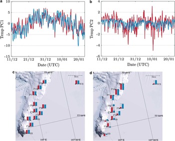
Figure 6a shows the first temperature PC of SNOW-WEB (red) and iAMPS (blue) interpolated values and Fig. 6c its corresponding EOF. EOFs are shown superimposed over a satellite image of the region such that spatial patterns can be readily interpreted. Red bars at node sites show the EOF of SNOW-WEB data, while blue bars show that of the corresponding iAMPS values. The first PC describes the diurnal cycle of the temperature data and the change due to the seasonal march. An increase is seen leading up to the New Year and a decrease succeeding it. EOF loadings show positive values across the entire network and are remarkably similar between SNOW-WEB and iAMPS. The correlation between the two PCs is also high at 0.81, with 74% (97%) of the variance of SNOW-WEB (iAMPS) contained within this EOF.
First two temperature principal components (PCs) and empirical orthogonal functions (EOFs) for SNOWWEB data (red) and iAMPS (blue) output. Dashed lines on EOF bar graphs represent 0.1 increments of an arbitrary scale. They are plotted for ease of comparison. a. PC1, b. PC2, c. EOF1, and d. EOF2.

The second PC and EOF are shown in Fig. 6b & d. The correlation between the iAMPS and SNOW-WEB PCs is still high at 0.58. However, the variance of the SNOW-WEB PC is much higher than that of iAMPS. The percentage of variance accounted for is 9% (2%) for SNOW-WEB (iAMPS). This EOF is interpreted to be the modulation of the diurnal cycle according to elevation and ground cover. SNOW-WEB nodes at high altitudes have large negative EOF values, as the amplitude of the diurnal cycle at these stations is decreased. Ice shelf nodes have amplified diurnal cycles due to the high albedo of the ice and enhanced night-time shading due to slopes to the north, hence the positive EOF loadings at these stations. iAMPS reproduces the spatial patterns adequately, but appears to load too lightly at stations near the base of the peninsula and too heavily at those further away.
The first two EOFs of SNOW-WEB (iAMPS) contain 83% (99%) of the spatial variance. It is clear that more spatial variability exists in the SNOW-WEB data than in iAMPS. However, the correspondence between the first two PCs and EOFs for SNOW-WEB and iAMPS is remarkably good.
EOF analysis on the wind speed (not shown) is much harder to interpret physically. However, results show remarkable similarity between the two datasets, particularly for the first two principal components which are correlated at 0.52 and 0.47, respectively. iAMPS over-represents the variance contained within the first EOF, with 55% observed in SNOW-WEB and 75% in iAMPS. However, the second EOF of both datasets contains 15% of the variance.
We have also performed varimax rotated EOF analysis, following Preisendorfer (Reference Preisendorfer1988) to examine whether the EOF patterns can be physically interpreted. Differences between rotated and unrotated EOFs are negligible. Thus, the presented EOFs are likely to represent physical modes of variation rather than mathematical artefacts.
Case study
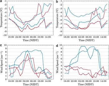
In order to highlight the respective advantages and disadvantages of the SNOW-WEB and iAMPS datasets, we present a short case study of temperature and wind measurements. For logistical purposes, the Ross Island region uses New Zealand Daylight Time (NZDT) in the summer months. As diurnal cycles are relavent in the coming section, we use NZDT from here on. Figure 7 shows temperature and scalar wind speed data series for nodes P6, P9, P2 and P10 of both SNOW-WEB and iAMPS datasets for the day-long period of 17h00 NZDT 20 January to 16h00 NZDT 21 January 2012. P6 and P9 are separated by c. 3.5 km on the ice shelf at the base of the Hut Point Peninsula. P6 is situated at the transition from flat ice to the peninsula slope, adjacent to the GPS route leading to ‘Room With a View’. P9 is located to the south-east of P6, on the Windless Bight route. P2 and P10 are situated at opposite ends of the network range, towards Scott Base and ‘Room With a View’, respectively. The distance between P2 and P10 is c. 12 km.We compare series for P6 and P9 to observe how iAMPS forecasts reproduce the data from two nodes that are very close together but in rather different topographical areas. We compare P2 and P10 to observe differences in iAMPS over larger distances. The time series presented is taken over a period of sustained and relatively strong winds from the north-west.
Time series of temperature and scalar wind speed for 17h00 New Zealand Daylight Time (NZDT) 20 January to 16h00 NZDT 21 January 2012. Solid lines show data for SNOW-WEB nodes. Lines with symbols in corresponding colours show equivalent iAMPS series. a. Temperature, P6 blue, P9 red. b. Temperature, P2 blue, P10 red. c. Wind speed, P6 blue, P9 red. d. Wind speed, P2 blue, P10 red.

Comparison between datasets shows that temperature series (Fig. 7a & b) are generally very similar, although SNOW-WEB temperatures are several degrees higher than those of iAMPS, reflecting the general biases discussed in the AMPS intercomparison section. Both datasets show a diurnal cycle at all nodes with a distinct minimum at around 01h00 NZDT. A maximum is observed at P9 and P10 at 20h00 in SNOW-WEB data, well before local midday. This coincides with a distinct wind speed minimum. It is possible that this peak is due to radiative heating of the radiation shield at these nodes. A similar anomalous peak is seen in the temperature records of P2 and P6 at 19h00. Other peaks in the temperature series coincide well with those at SB (not shown), suggesting that they are representative of air temperature. iAMPS temperature series are similar to SNOW-WEB for P6 and P9 (Fig. 7a). Temperature series are also similar across datasets for P2 and P10 (Fig. 7b), although P2 is somewhat warmer than its iAMPS counterpart. Between 12h00 and 13h00, iAMPS shows a large decrease in temperature that is not seen in SNOW-WEB data. This shift in the iAMPS temperature seems to be caused by the discontinuity introduced by switching across AMPS forecasts and highlights a deficiency in the technique used to compile AMPS time series. A similar discontinuity is observed for iAMPS P2 between 00h00 and 01h00. Discontinuities are not observed in iAMPS wind series.
Temperatures at P6 and P9 appear to be more similar in iAMPS output compared to SNOW-WEB. To quantitatively assess the spatial variability of the temperature series we compute the root-mean-squared (RMS) temperature differences between P6 and P9 for SNOW-WEB and iAMPS. Anomalous peaks in the SNOW-WEB data are removed so as to reduce the influence of heating of radiation shields. SNOW-WEB shows an RMS difference of 1.2°C, while that of iAMPS is 0.7°C, implying that in this case, SNOW-WEB temperatures vary more rapidly with distance than iAMPS. Reduced variability observed in iAMPS is not a product of overlap of the interpolation routine. P6 and P9 do not share any AMPS grid points in their respective interpolations. This suggests that small-scale meteorological differences are not well-simulated in AMPS, due to smoothing across grid cells. The temperature bias between P2 and P10 in iAMPS is more pronounced, reflecting the larger distance between the two nodes. SNOW-WEB records, however, still show a larger bias. The RMS difference value between these nodes for SNOW-WEB (iAMPS) is 2.5°C (1.3°C).
Wind speeds vary more greatly between datasets, particularly at P6 and P9 (Fig. 7c). Strong flow from the north-west is represented in both, but the onset of high winds in iAMPS is later and more sudden than in SNOW-WEB at these nodes. iAMPS shows sharp increases in wind speed at both nodes at around 00h00. Speeds peak and rapidly decline by 07h00. iAMPS winds at P9 are reduced relative to P6, but the timing of peaks and troughs is very similar. In contrast, the SNOW-WEB series show a sudden onset of high winds at P6 at around 19h00, five hours before the increase seen in iAMPS. The wind at this node remains strong until its rapid decline between 11h00 and 12h00. The increase of wind is more gradual at P9. It peaks at 06h00 and declines over the course of the succeeding hour, well before the decline at P6. Wind speed at P9 is consistently lower than at P6. Comparing RMS differences again, we see that SNOW-WEB has a magnitude of 3.5 m s-1 over the period, while that of iAMPS is reduced at 1.2 m s-1.
The difference between wind speeds is much better represented at P2 and P10 (Fig. 7d), the more distant of the comparison pairs. Winds at these nodes are forecast very well during this time, with P10 showing a gradual decline in speeds up to 08h00, and a large sustained peak at P2. The onset of high winds at P2 is later in iAMPS, however. Both datasets show large biases between wind speed at P2 and P10. The RMS difference between P2 and P10 is 4.7 m s-1 (5.0 m s-1) for SNOW-WEB (iAMPS), suggesting that iAMPS represents variation in wind speed more accurately at larger distances. Wind directions are reproduced well throughout the event, particularly during the periods of strongest wind.
These results show that temperature variation with distance is more pronounced in SNOW-WEB over AMPS at both scales inspected. Wind speed variation is more accurately matched. The ability of AMPS to predict biases in wind speed is dependent upon its ability to resolve differences in topography. For larger distances this seems to be resolved rather well, with accurate biases well matched between datasets. However, the bias between P6 and P9, which are close together in space but rather different in terms of topography, is under-represented in iAMPS. The distributed nature of SNOW-WEB allows us to observe these effects in detail.
Summary
SNOW-WEB is a meteorological monitoring system, novel both in its electronic and mechanical design, that has the potential to overcome several drawbacks of conventional Antarctic weather stations. Field testing has shown that the concept of a lightweight, easily deployable, and cost-effective network of weather stations is a viable one. Although the design has only been tested in summer in the Antarctic, the ease with which the nodes can be erected, particularly the secondary design, was considered a success. Development must now be undertaken to ensure the network is capable of lasting the long Antarctic winter and is more robust to failure. Power generation was not problematic for the summer field tests, but will prove a challenge for the future of the project. Large battery banks and wind turbines are being considered as solutions.
The networking aspect of the project has proved itself viable in Antarctica. A significant quantity of meteorological and GPS data were transferred wirelessly to Scott Base over the course of the deployment. Nodes were also controlled remotely from the base in real-time using a mesh-network. To our knowledge, this is a first in Antarctic weather station systems. Development must be carried out on the logging firmware of the devices to ensure fewer stalled nodes in the future and prevent problems originating in individual nodes from flooding the network. A long-term test of the firmware must be carried out before the next field season. Work must also be performed on the networking component of the project to produce a more robust mesh, capable of operating unsupervised for months at a time.
We have performed statistical data validation on the collected meteorological data using established sources. Firstly, verification was carried out using AWS data from the surrounding region. SNOW-WEB data has been shown to correlate well with AWS data and mean and standard deviation statistics are similar. Comparison has also been performed using AMPS forecast records. AMPS forecasts for the summer of 2011/12 show high correlations with SNOW-WEB data and that of established weather stations, and biases are generally low. Comparison statistics for SNOW-WEB are approximately the same as those for the established weather stations, suggesting that SNOW-WEB data is as reliable as that of weather stations already operating in the region. EOF analysis of SNOW-WEB and forecast data shows a high degree of similarity, acting to reinforce the validity of both SNOW-WEB and AMPS data. We have shown that the latest generation of AMPS has probably improved summertime wind prediction capabilities in this region. However, computed biases only describe the reproduction in AMPS of the prevailing conditions. Wind roses show several smaller peaks in wind direction. It is these less frequent peaks that represent the periods of high winds that may ground aircraft or prevent landings at runways near the tip of the peninsula. Following Nigro et al. (Reference Nigro, Cassano and Seefeldt2011), a more detailed analysis of AMPS predictions in the region and their variation with wind regimes is planned.
Deficiencies have become apparent in AMPS, SNOW-WEB and AWS datasets. A simple case study has highlighted that the resolution and extent of SNOW-WEB allows the recording of local-scale processes that are not simulated well in the AMPS record because the spatial variation of the data is too smooth. However, analysis of temperature differences according to wind speed has shown that SNOW-WEB and other AWS units in the region suffer from large positive biases due to direct radiative heating of radiation shields. This effect is amplified at times when wind speeds are low as air stagnates within the radiation shields and generates a warm region around the temperature sensor. Concerning the validation of SNOW-WEB data, this is a drawback but one from which a large number of Antarctic AWS units also suffer. We are considering the inclusion of artificially aspirated radiation shields to prevent warm air stagnation for future generations of SNOW-WEB. Aspirated shields represent a significant increase in power consumption, but they would only be required to function in the summertime when ample light is available for power generation.
We conclude that with careful interpretation SNOW-WEB data from the 2011/12 field season can be usefully employed in the study of mesoscale meteorology in the area surrounding the Hut Point Peninsula. However, given the caveats of SNOW-WEB and AMPS data specified above, it is clearly advantageous to employ a combination of data types. We intend to utilize the summer field season data in dynamical studies of the area and perform high-resolution model validation, such that the mesoscale meteorology of the region can be further understood.
Acknowledgements
Thanks go to the staff of Antarctica New Zealand and Scott Base, for logistical support over the course of the project, especially to Hayden Short for invaluable aid in SNOW-WEB deployment. We would also like to acknowledge the support of NIWA and the University of Wisconsin, Madison, for providing AWS data, and Kevin Manning at UCAR for providing AMPS forecast output for the experimental period. Finally, we wish to thank Holly Painter for her proof-reading services, and two anomymous reviewers for suggestions on the manuscript.