

1 Introduction
The DARPA suboff body (DSub) is a notional geometry, which has been utilized in several studies targeting fluid dynamics phenomena relevant to underwater vehicles. Huang et al. (Reference Huang, Liu, Groves, Forlini, Blanton and Gowing1992) carried out detailed measurements in several configurations, including appendages and wing rings, although most results were provided for the bare hull case. Their findings pointed to the complexity of the flow over the stern, where the boundary layer experiences the effect of a strong adverse pressure gradient. A more recent experimental study by Jiménez, Hultmark & Smits (Reference Jiménez, Hultmark and Smits2010a) reported measurements in the wake of the DSub for Reynolds numbers up to  $Re_{L}=U_{\infty }L/\unicode[STIX]{x1D708}=67\times 10^{6}$ (
 $U_{\infty }$ is the free-stream velocity,
 $L$ the length of the DSub and
 $\unicode[STIX]{x1D708}$ the kinematic viscosity of the fluid), showing the presence of distinct peaks of turbulent fluctuations away from the wake axis. Jiménez, Reynolds & Smits (Reference Jiménez, Reynolds and Smits2010b) verified also that this flow feature was reinforced by the presence of fins in the wake of the appended DSub. They conjectured that the bimodal distribution of the turbulent stresses in the wake originated from the thick boundary layer over the stern. However, they did not report measurements of the stern boundary layer.
Numerous computational studies on the towed DSub configuration are available in the literature, where usually the Reynolds-averaged Navier–Stokes (RANS) equations are solved due to cost considerations (Gorski, Coleman & Haussling Reference Gorski, Coleman and Haussling1990; Givler et al. Reference Givler, Gartling, Engelman and Haroutunian1991; Boger & Dreyer Reference Boger and Dreyer2006; Toxopeus Reference Toxopeus2008; Pan, Zhang & Zhou Reference Pan, Zhang and Zhou2012; Budak & Beji Reference Budak and Beji2016; Cao, Zhu & Zeng Reference Cao, Zhu and Zeng2016; Manshadi, Hejranfar & Farajollahi Reference Manshadi, Hejranfar and Farajollahi2017; Gao et al. Reference Gao, Wang, Pang, Chen and Tang2018; Wang et al. Reference Wang, Gao, Pang and Tang2018; Zhang, Chao & Pan Reference Zhang, Chao and Pan2019), with some works dealing also with the free-surface effects (Shariati & Mousavizadegan Reference Shariati and Mousavizadegan2017; Amiri et al. Reference Amiri, Esperana, Vitola and Sphaier2018). More recently, hybrid formulations such as the detached eddy simulation (DES) approach are gradually replacing RANS in the design cycle. In this case, the boundary layers on the DSub body are still captured using RANS, but large-eddy simulation (LES) is used in the wake (see, for example, Vaz, Toxopeus & Holmes Reference Vaz, Toxopeus and Holmes2010; Zhihua, Ying & Chengxu Reference Zhihua, Ying and Chengxu2011, Reference Zhihua, Ying and Chengxu2012; Bhushan, Alam & Walters Reference Bhushan, Alam and Walters2013; Chase, Michael & Carrica Reference Chase, Michael and Carrica2013; Chase & Carrica Reference Chase and Carrica2013; Kim & Rhee Reference Kim and Rhee2016). Due to cost considerations LESs were only recently introduced, targeting fairly low Reynolds numbers (Mahesh et al. Reference Mahesh, Kumar, Gnanaskandan and Nitzkorski2015; Posa & Balaras Reference Posa and Balaras2016a; Wang et al. Reference Wang, Shi, Li and He2016; Kumar & Mahesh Reference Kumar and Mahesh2018a,Reference Kumar and Maheshb), or utilizing coarse grids that cannot capture the full range of scales (Alin et al. Reference Alin, Bensow, Fureby, Huuva and Svennberg2010; Feng et al. Reference Feng, Wang, Jiang and Zhang2015; Yao et al. Reference Yao, Zhang, Liu and Jiang2017).
In particular, Posa & Balaras (Reference Posa and Balaras2016a) reported wall-resolved LES for the towed DSub configuration at  $Re_{L}=1.2\times 10^{6}$. The results confirmed the complexity of the stern flow and traced the source of the bimodal behaviour of the turbulent stresses in the wake back to the thick boundary layer at the rear of the DSub. The computations also confirmed the experimental observations by Jiménez et al. (Reference Jiménez, Reynolds and Smits2010b), that the junction vortices reinforce the bimodal distribution of the stresses by enhancing turbulence in the boundary layer. The turbulent boundary layer over the cylindrical mid-body, on the other hand, was found to be practically in equilibrium, following closely the growth rate of a zero pressure gradient turbulent boundary layer (ZPGTBL). In a follow up paper Posa & Balaras (Reference Posa and Balaras2016b) considered a self-propelled configuration, where the propulsor was also included in the computation. A strong interaction of the propulsor with the stern flow was demonstrated, while the equilibrium region of the boundary layer further upstream was practically unaffected. Wang et al. (Reference Wang, Shi, Li and He2016) considered the same geometry at a slightly lower Reynolds number,
 $Re_{L}=1.0\times 10^{6}$. Their study focused on the feasibility of LES, coupled with a diffuse-interface immersed-boundary (IB) formulation, such as the one proposed by Shi et al. (Reference Shi, Yang, Jin, He and Wang2019). In the latter, for the first time wall modelling is proposed in the framework of a diffuse-interface IB technique. They reported results in good agreement with the experiments by Huang et al. (Reference Huang, Liu, Groves, Forlini, Blanton and Gowing1992) and the LES solutions by Posa & Balaras (Reference Posa and Balaras2016a).
Recently, Kumar & Mahesh (Reference Kumar and Mahesh2018a,Reference Kumar and Maheshb) carried out wall-resolved LES on the barehull DSub without sail or stern appendages at  $Re_{L}=1.1\times 10^{6}$. They found good agreement with available experiments (Huang et al. Reference Huang, Liu, Groves, Forlini, Blanton and Gowing1992) on the same geometry, as well as the wall-resolved LES on the appended DSub reported earlier (Posa & Balaras Reference Posa and Balaras2016a). They confirmed the fast evolution to self-similarity by first-order statistics, in contrast with the second-order statistics, which take further streamwise development downstream. In addition, they verified the presence of maxima of turbulent kinetic energy in the wake away from its axis, confirming that this feature develops even in absence of stern appendages, coming primarily from the stern boundary layer. However, in these computations the Reynolds number was fairly low and similar to the one considered by Posa & Balaras (Reference Posa and Balaras2016a).
In the present study we report wall-resolved LES at a Reynolds number increased by an order of magnitude to  $Re_{L}=12\times 10^{6}$. The strategy we followed to enable such a dramatic increase in the Reynolds number was guided by the simulations reported by Posa & Balaras (Reference Posa and Balaras2016a), where it was observed that the turbulent boundary layer over the cylindrical mid-body was practically in equilibrium. As such, we adopted a wall-modelling strategy for most of the cylindrical mid-body to reduce the cost and provide high-quality boundary conditions to the downstream computational domain, where the grid was refined to the standards of wall-resolved LES. The main focus is on the effects of the Reynolds number on various flow features along the stern and near wake. These will be established by comparing the present results to the computations at
 $Re_{L}=1.2\times 10^{6}$, reported in Posa & Balaras (Reference Posa and Balaras2016a). Particular emphasis will be placed on the role of the junction vortices and how their dynamics is affected by the Reynolds number, as the current understanding is rather limited. We will show that the flow over the stern is dominated by the adverse streamwise pressure gradient and is weakly dependent on the Reynolds number. The circulation of the junction vortices, however, experienced an increase with the Reynolds number and their role in feeding turbulence to the stern boundary layer was enhanced. This behaviour balanced the lower turbulent kinetic energy within the stern boundary layer at the higher Reynolds number, resulting in similar values for the maxima of turbulent kinetic energy within the wake of the DSub between the two simulated Reynolds numbers.
The paper is organized as follows: in § 2 the numerical approach is discussed, including the wall-modelling strategy; details of the computational set-up are reported in § 3; in § 4 validation, via comparison with experiments in the literature at  $Re_{L}=12\times 10^{6}$, is provided. Then the flow physics on both the stern boundary layer and wake flow are analysed, including comparisons with results at
 $Re_{L}=1.2\times 10^{6}$; conclusions are given in § 5.
2 Methodology
In LES the dynamics of the resolved scales is governed by the filtered Navier–Stokes equations for incompressible flow,
 $$\begin{eqnarray}\displaystyle & \displaystyle \frac{\unicode[STIX]{x2202}\tilde{u} _{i}}{\unicode[STIX]{x2202}x_{i}}=0, & \displaystyle\end{eqnarray}$$
 $$\begin{eqnarray}\displaystyle & \displaystyle \frac{\unicode[STIX]{x2202}\tilde{u} _{i}}{\unicode[STIX]{x2202}t}+\frac{\unicode[STIX]{x2202}\tilde{u} _{i}\tilde{u} _{j}}{\unicode[STIX]{x2202}x_{j}}=-\frac{\unicode[STIX]{x2202}\tilde{p}}{\unicode[STIX]{x2202}x_{i}}-\frac{\unicode[STIX]{x2202}\unicode[STIX]{x1D70F}_{ij}}{\unicode[STIX]{x2202}x_{j}}+\frac{1}{Re_{L}}\frac{\unicode[STIX]{x2202}^{2}\tilde{u} _{i}}{\unicode[STIX]{x2202}x_{j}^{2}}+f_{i}, & \displaystyle\end{eqnarray}$$
where  $\langle {\sim}\rangle$ indicates filtered quantities;
 $u_{i}$ and
 $x_{i}$ are the velocity and spatial coordinate in the
 $i$th direction, respectively;
 $t$ stands for time and
 $p$ for pressure. The subgrid scales stress (SGS) tensor,
 $\unicode[STIX]{x1D70F}_{ij}$, represents the effect of the unresolved scales and was parameterized using the wall-adapting local eddy-viscosity (WALE) model by Nicoud & Ducros (Reference Nicoud and Ducros1999). The forcing term,
 $f_{i}$, was utilized in the framework of the IB method to enforce the no-slip boundary condition on the surface of the DSub (Balaras Reference Balaras2004; Yang & Balaras Reference Yang and Balaras2006). The equations were advanced in time using a fractional step method, and all spatial derivatives were discretized with second-order central differences on a staggered cylindrical coordinates grid. The viscous and convective terms of the azimuthal derivatives were treated implicitly using the Crank–Nicolson scheme. All other terms were advanced with an explicit three-step Runge–Kutta scheme. The resulting Poisson equation was solved using a direct solver based on a divide and conquer strategy (Rossi & Toivanen Reference Rossi and Toivanen1999). Details on the overall formulation can be found in Balaras (Reference Balaras2004) and Yang & Balaras (Reference Yang and Balaras2006), while the implementation details and parallel efficiency for problems of similar size are outlined in Beratlis, Squires & Balaras (Reference Beratlis, Squires and Balaras2012). A demonstration of the accuracy and efficiency of the solver in naval hydrodynamics can be found in Schroeder, Posa & Balaras (Reference Schroeder, Posa and Balaras2014), Balaras, Schroeder & Posa (Reference Balaras, Schroeder and Posa2015), Posa & Balaras (Reference Posa and Balaras2016a,Reference Posa and Balarasb, Reference Posa and Balaras2018), Posa et al. (Reference Posa, Broglia, Felli, Falchi and Balaras2018), Posa, Broglia & Balaras (Reference Posa, Broglia and Balaras2019a,Reference Posa, Broglia and Balarasb) and Posa et al. (Reference Posa, Broglia, Felli, Falchi and Balaras2019c).
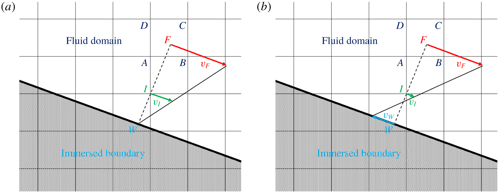
(a) Linear velocity reconstruction at the interface node  $\boldsymbol{I}$ between the wall and the fluid domain; (b) slip wall on the immersed boundary,
 $\boldsymbol{v}_{\boldsymbol{W}}$, correcting the linear reconstruction in
 $\boldsymbol{I}$ in order to compensate for the lost momentum flux, due to under-resolution in the inner layer region.

Central to the implementation of the IB method utilized in this study is the reconstruction of the velocity near the body at computational nodes that are in the fluid phase, but have at least one neighbour in the solid (see figure 1). When the grid resolution is sufficient to place a number of points in the viscous sub-layer, then the linear reconstruction proposed in Balaras (Reference Balaras2004) is accurate. It is illustrated in figure 1(a), where the velocity boundary condition at  $\boldsymbol{I}$,
 $\boldsymbol{v}_{\boldsymbol{I}}$, is interpolated linearly between the projection of the interface node
 $\boldsymbol{I}$ on the surface of the immersed boundary, indicated by
 $\boldsymbol{W}$, and the fluid point
 $\boldsymbol{F}$, along the direction normal to the wall. Since in general
 $\boldsymbol{F}$ is not a grid node, the fluid velocity there,
 $\boldsymbol{v}_{\boldsymbol{F}}$, needs to be interpolated considering the neighbouring grid nodes
 $\boldsymbol{A}$,
 $\boldsymbol{B}$,
 $\boldsymbol{C}$ and
 $\boldsymbol{D}$. For the range of Reynolds numbers considered in the present work, resolving the boundary layers upstream of the stern is prohibitively expensive and the grid is designed to resolve the outer layer only. As a result, point
 $\boldsymbol{I}$ is practically located in the logarithmic layer and the linear reconstruction described above leads to large errors. To address this issue a wall-modelling strategy is used. In particular, the velocity at the fluid point
 $\boldsymbol{F}$ is the input to the standard log law (Spalding Reference Spalding1961):
 $$\begin{eqnarray}y^{+}=v^{+}+\text{e}^{-B\unicode[STIX]{x1D705}}[\text{e}^{\unicode[STIX]{x1D705}v^{+}}-1-\unicode[STIX]{x1D705}v^{+}-(\unicode[STIX]{x1D705}v^{+})^{2}/2!-(\unicode[STIX]{x1D705}v^{+})^{3}/3!-(\unicode[STIX]{x1D705}v^{+})^{4}/4!],\end{eqnarray}$$
where  $y^{+}$ and
 $v^{+}$ are the distance and the tangential velocity in wall units, and
 $k=0.41$,
 $B=5.0$. Note that
 $y^{+}=yu_{\unicode[STIX]{x1D70F}}/\unicode[STIX]{x1D708}$,
 $v^{+}=v/u_{\unicode[STIX]{x1D70F}}$ and
 $u_{\unicode[STIX]{x1D70F}}=\sqrt{\unicode[STIX]{x1D70F}_{w}/\unicode[STIX]{x1D70C}}$, with
 $\unicode[STIX]{x1D70F}_{w}$ and
 $\unicode[STIX]{x1D70C}$ standing for the wall stress and the fluid density, respectively. Equation (2.3) is then solved using an iterative Newton–Raphson procedure to compute the wall stress,
 $\unicode[STIX]{x1D70F}_{w}^{sol}$. The initial guess in this process is the wall stress computed from a provisional linear reconstruction of the solution, while convergence is achieved when the error is less than 10-8. To avoid excessive fluctuations of the estimated wall shear stress, local averaging along the azimuthal direction was performed at point
 $\boldsymbol{F}$.
Next, the velocity  $\boldsymbol{v}_{\boldsymbol{I}}$ at point
 $\boldsymbol{I}$ can be estimated from the log law. This would be the final step in the implementation of an equilibrium wall model in a classical boundary conforming method. In the case of an IB formulation, however, setting the velocity
 $\boldsymbol{v}_{\boldsymbol{I}}$ to the proper value does not guarantee that the viscous flux at the wall will be correct: other quantities within the finite-difference operators, such as the turbulent viscosity, need to be adjusted (see Balaras Reference Balaras2004, for a discussion). Depending on the geometry, this can be a complex process, which may impact accuracy and robustness. To keep such errors small enough, in the present work we introduce the following control strategy: the value
 $\unicode[STIX]{x1D70F}_{w}^{sol}$, which is consistent with the initial reconstruction from the log law, is compared to a reference one,
 $\unicode[STIX]{x1D70F}_{w}^{ref}$, to define the error,
 $e=\unicode[STIX]{x1D70F}_{w}^{ref}-\unicode[STIX]{x1D70F}_{w}^{sol}$. The reference wall stress is estimated from the wall-resolved LES at a lower Reynolds number,
 $Re_{L}=1.2\times 10^{6}$, by scaling it to account for the difference between the two Reynolds numbers (
 $\unicode[STIX]{x1D70F}_{w}\propto Re_{L}^{-0.2}$). The error is then utilized as input to a proportional–integral (PI) controller to define a negative slip-wall velocity,
 $\boldsymbol{v}_{\boldsymbol{W}}$, and adjust the velocity at the interface node
 $\boldsymbol{I}$ (figure 1b). As a result, the PI controller dynamically adjusts the slip-wall velocity,
 $\boldsymbol{v}_{\boldsymbol{W}}$, in order for the outer layer to match the target wall stress, based on the velocity at the fluid point
 $\boldsymbol{F}$ and the log law
 $$\begin{eqnarray}\boldsymbol{v}_{\boldsymbol{W}}=P\unicode[STIX]{x1D716}+I\int _{0}^{t}\unicode[STIX]{x1D716}\,\text{d}t,\end{eqnarray}$$
where  $P$ and
 $I$ are the constants of the proportional and integral components of the controller that, in the present study, were both selected equal to 10, while
 $\unicode[STIX]{x1D716}$ is the relative error, computed as
 $\unicode[STIX]{x1D716}=e/\unicode[STIX]{x1D70F}_{w}^{ref}$. The proportional and integral constants of the controller were modified empirically during the computations in order to achieve a quick response of the controller, still able to avoid instabilities of the solution and large overshooting behaviours of
 $\unicode[STIX]{x1D70F}_{w}^{sol}$, relative to
 $\unicode[STIX]{x1D70F}_{w}^{ref}$, to accelerate the establishment of a statistically steady solution in line with the target value for the wall stress.
It is worth noting that the availability of a reference value,  $\unicode[STIX]{x1D70F}_{w}^{ref}$, is critical for the accuracy of the above strategy. In the present case, it comes from the earlier wall-resolved LES (Posa & Balaras Reference Posa and Balaras2016a), where we also observed that the boundary layer over the surface of the mid-body behaves as a ZPGTBL. The adaptation of the model to flows where this information is not directly available, but can be estimated, is possible, but is beyond the scope of the present work.
3 Set-up of the computations
The design of the present computations is driven by our prior wall-resolved LES of the same geometry in towed (Posa & Balaras Reference Posa and Balaras2016a) and self-propelled (Posa & Balaras Reference Posa and Balaras2018) configurations at  $Re_{L}=1.2\times 10^{6}$. These computations demonstrated that the turbulent boundary layer over most of the DSub body is in equilibrium and it is the stern geometry that introduces significant pressure gradients, affecting the evolution of the boundary layers as well as the near-wake structure. The presence of the appendages and resulting junction flows adds to the complexity. In addition, in Posa & Balaras (Reference Posa and Balaras2018) we verified that the interaction between the propeller and the stern flow is also very strong, while the rest of the boundary layer upstream of the stern is practically unaffected. Based on these findings we chose to focus the computational resources at the stern and in the near-wake area, where the highest fidelity is required in the present computations at a much higher Reynolds number,
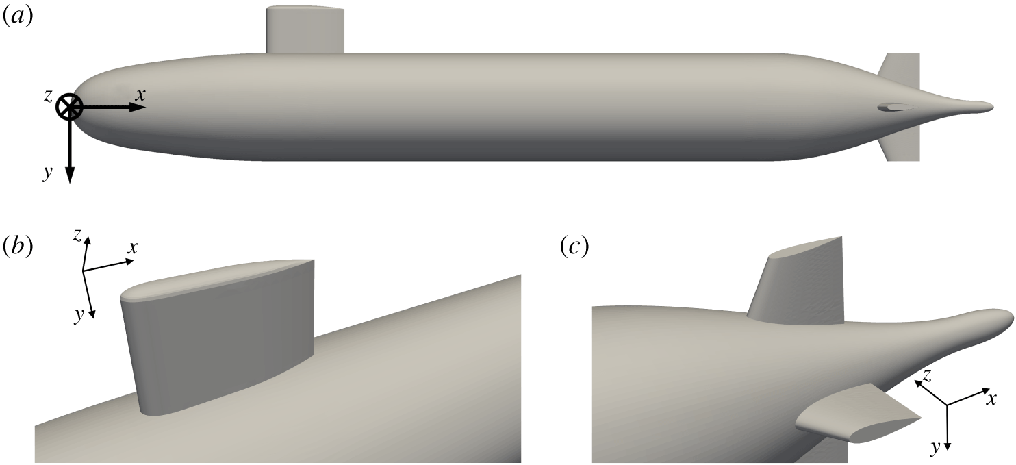
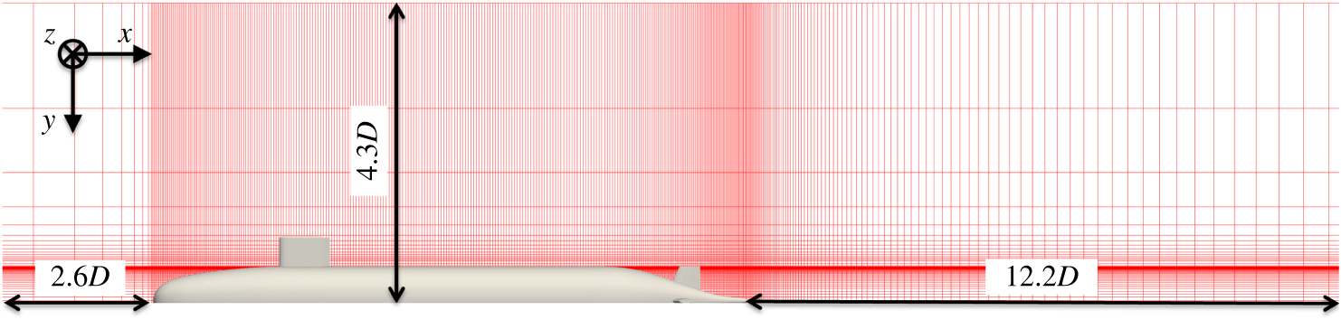
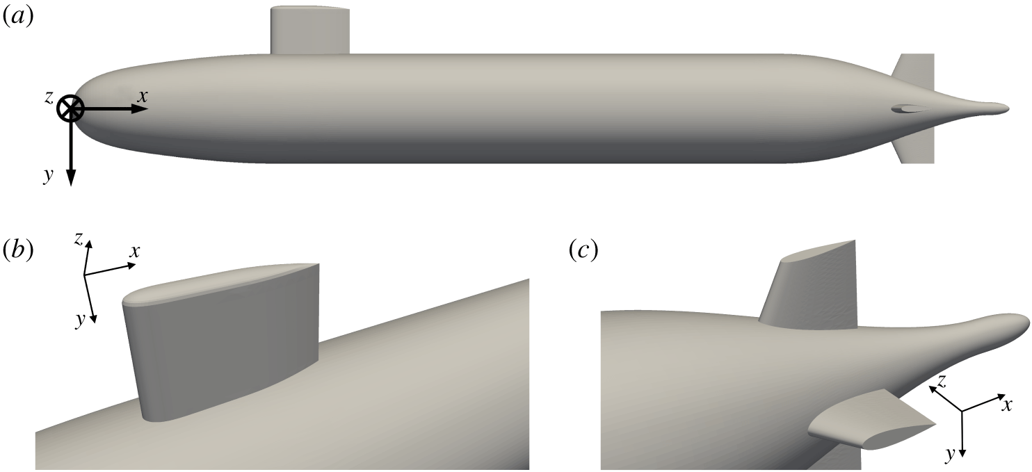
 $Re_{L}=12\times 10^{6}$. The geometry of the appended DSub is shown in figure 2, including the sail and four stern fins. The size of the computational domain is reported in figure 3, where also a meridian slice of the computational grid is shown (only 1 of every 16 points plotted).
(a) Full geometry of the appended DSub; (b) detail of sail; (c) detail of fins.
A numerical trip wire was used to force transition to turbulence at approximately the same location as in the reference experiments (approximately  $0.25D$ from the nose of the DSub as in Huang et al. Reference Huang, Liu, Groves, Forlini, Blanton and Gowing1992 and Jiménez et al. Reference Jiménez, Hultmark and Smits2010a,Reference Jiménez, Reynolds and Smitsb). It was introduced by IB forcing, where the no-slip condition was enforced within a few cells of the computational grid. The extent of this region across the cross-stream and streamwise directions was selected roughly equal to the diameter of the physical trip wire adopted in the experiments, corresponding to approximately 1 % of the diameter of the DSub. This forcing was distributed across the whole azimuthal extent of the bow. The numerical trip wire acts as the one in the experiments, triggering transition of the boundary layer via local separation, followed by turbulent reattachment. The implementation details can be found in Posa & Balaras (Reference Posa and Balaras2016a).
Computational domain and a meridian slice of the computational grid (1 in every 16 nodes shown).

The conditions at the boundaries of the computational domain are a uniform velocity at the inlet, convective at the outlet (Orlanski Reference Orlanski1976) and free slip at the radial boundaries. No-slip conditions or the wall-modelling strategy discussed above were used on the DSub walls. In particular, the wall model was activated just after the trip wire and deactivated at the beginning of the stern. The grid resolution was adjusted to satisfy the requirements for wall-modelled LES in the section  $0.25D<x<0.70D$: the first point was placed in the log layer and the average resolution within the outer layer was 303 points in each
 $\unicode[STIX]{x1D6FF}^{3}$, with
 $\unicode[STIX]{x1D6FF}$ standing for the boundary layer thickness. In the stern area, where the boundary layer is much thicker, the grid resolution was adjusted to be compatible with wall-resolved LES. Overall, the cylindrical coordinate grid was composed of
 $902\times 1502\times 6002$ (8.1 billion) nodes along the radial, azimuthal and axial directions, respectively. At the mid-bow, 140 nodes were placed within the turbulent boundary layer. Along the stern, at the streamwise location corresponding to 86 % of the DSub length, upstream of the stern appendages, the number of nodes within the boundary layer was equal to 235, while at 90 % of the DSub length, between the stern appendages, the number of grid nodes was 275.
The computations were carried out on 3000 cores of a Cray XC40 cluster, featuring 2.3 GHz Intel Xeon E5-2698 v3 cores. The computational grid was decomposed into cylindrical subdomains, splitting the overall problem across the streamwise direction, using a message passing interface strategy to handle communications across subdomains. Computations were carried out for more than 2 flow-through times, requiring a wall clock time of approximately 1 month, with an overall cost of approximately 2 million CPU hours. All statistics presented in the next sections were computed during the second flow-through time, when transients were washed out. We found that this statistical sample is sufficient for converged first- and second-order statistics. Increasing the sample certainly results in smoother profiles, but it does not affect the quantitative comparisons with the experiments or the analysis of the results. The maximum difference in the velocity root mean squares, for example, when the sample size was increased from 0.5 flow-through times to 1.0 flow-through times, was found to be less than 5 %. We should also note that most of the statistics were computed on-the-fly, enabling us to sample approximately 70 000 realizations during one flow-through time.
4 Results
4.1 Validation
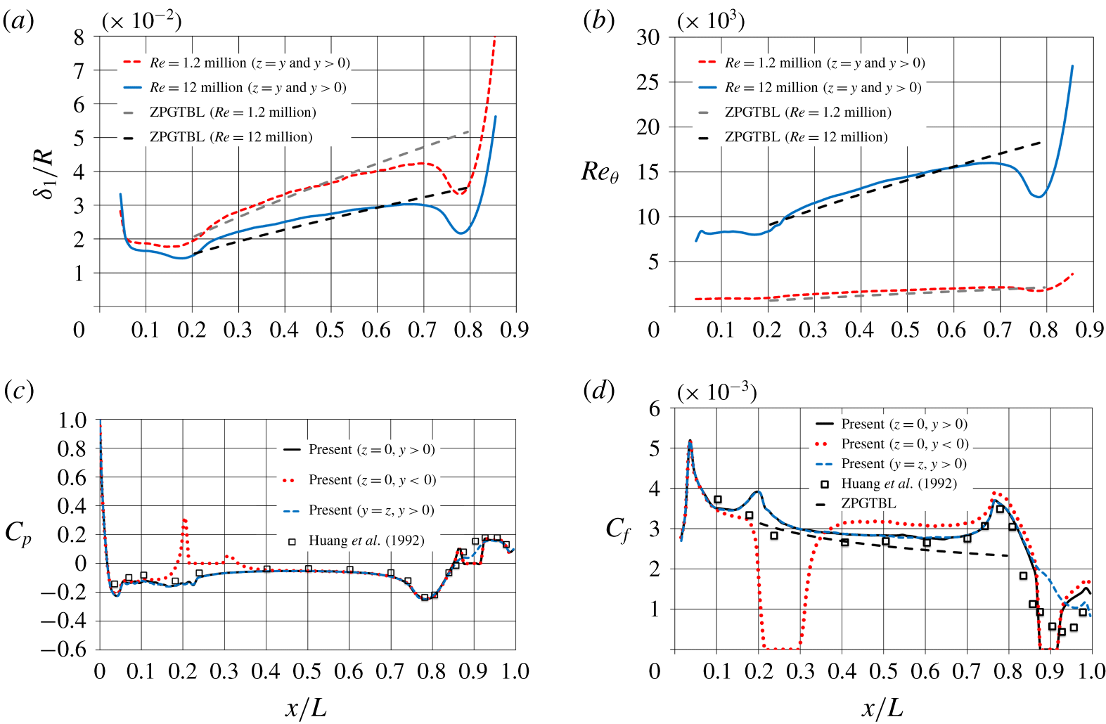
The growth of the boundary layer along the DSub body is illustrated in figure 4(a,b), where the evolution of the displacement thickness,  $\unicode[STIX]{x1D6FF}_{1}$, and momentum thickness Reynolds number,
 $Re_{\unicode[STIX]{x1D703}}=\unicode[STIX]{x1D6FF}_{2}U_{\infty }/\unicode[STIX]{x1D708}$ (
 $\unicode[STIX]{x1D6FF}_{2}$ stands for momentum thickness) are shown. The results at the lower Reynolds number,
 $Re_{L}=1.2\times 10^{6}$, reported in Posa & Balaras (Reference Posa and Balaras2016a), are added for comparison together with the slope for the case of a ZPGTBL. For both wall-resolved and wall-modelled simulations the evolution of
 $\unicode[STIX]{x1D6FF}_{1}$ and
 $Re_{\unicode[STIX]{x1D703}}$ for the cylindrical part of the geometry (
 $0.25D<x<0.7D$) agrees with the ZPGTBL slope. As expected, the boundary layer is thinner at
 $Re_{L}=12\times 10^{6}$ and the momentum thickness Reynolds number is larger. For instance, at the mid-body location the displacement thickness is equal to
 $\unicode[STIX]{x1D6FF}_{1}/R\approx 0.0366$ and
 $\unicode[STIX]{x1D6FF}_{1}/R\approx 0.0275$ for
 $Re_{L}=1.2\times 10^{6}$ and
 $Re_{L}=12\times 10^{6}$, respectively. At the same position along the hull the momentum thickness Reynolds numbers are equal to
 $Re_{\unicode[STIX]{x1D703}}\approx 1840$ and
 $Re_{\unicode[STIX]{x1D703}}\approx 14\,470$ for the two cases.
Time-averaged distribution of: (a) displacement thickness; (b) momentum thickness Reynolds number; (c) pressure coefficient,  $C_{p}$; (d) skin-friction coefficient,
 $C_{f}$. Here
 $R$ denotes the radius of the cylindrical mid-body.

In figure 4(c,d) the time-averaged distributions of pressure coefficient,  $C_{p}=(p-p_{\infty })/(0.5\unicode[STIX]{x1D70C}U_{\infty }^{2})$, and skin-friction coefficient,
 $C_{f}=\unicode[STIX]{x1D70F}_{w}/(0.5\unicode[STIX]{x1D70C}U_{\infty }^{2})$, where
 $p_{\infty }$ is the free-stream pressure, are compared to the experimental results by Huang et al. (Reference Huang, Liu, Groves, Forlini, Blanton and Gowing1992) for a bare hull DSub. The LES results are shown at three azimuthal coordinates to illuminate the effect of both sail and stern appendages. Over the mid-body the agreement of
 $C_{p}$ and
 $C_{f}$ with the experimental data is very good in the two planes away from the sail. Downstream of the sail
 $C_{f}$ is higher, due to the presence of the junction vortices. As we will discuss below in detail, they originate at the root of the sail and bring higher momentum fluid towards its wake from the outer layer at azimuthal locations away from the plane of the appendage. This effect is also distinguishable over the upstream region of the stern, where the skin friction remains slightly higher than at the other azimuthal locations. An acceleration of the boundary layer is generated at the convex edge between cylindrical mid-body and stern (
 $x/L\approx 0.75$), as confirmed by the distribution of the pressure coefficient and the close agreement between computations and experiments. In the present results this is also evident at the edge between bow and cylindrical mid-body (
 $x/L\approx 0.2$), where the local maximum is higher than in the experiments by Huang et al. (Reference Huang, Liu, Groves, Forlini, Blanton and Gowing1992). This may be due to the influence of the sail, generating additional blockage, compared to the bare hull configuration of the measurements.
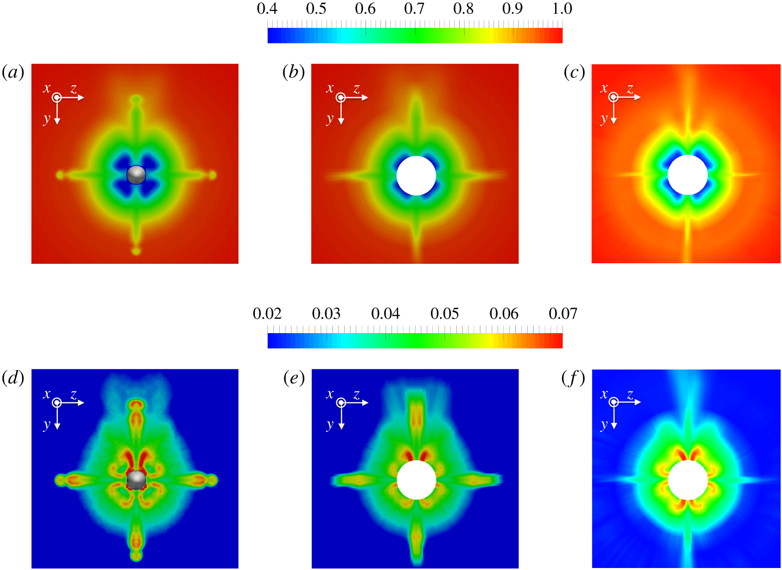
Contours of time-averaged streamwise velocity,  $u_{x}/U_{\infty }$ (a–c) and its root mean square,
 $u_{x}^{\prime }/U_{\infty }$ (d–f) for a cross-section at
 $x/L=0.978$: (a,d) computation on the original grid; (b,e) computation interpolated on the same grid utilized in the experiments; (c,f) measurements by Huang et al. (Reference Huang, Liu, Groves, Forlini, Blanton and Gowing1992).

A comparison of the velocity statistics with the measurements by Huang et al. (Reference Huang, Liu, Groves, Forlini, Blanton and Gowing1992) on the appended DSub is shown in figure 5. Both time-averaged and root mean square fluctuations of the streamwise velocity over a cross-section at  $x/L\approx 0.978$ near the tail of the body are plotted. When the computational results are interpolated on the same grid adopted to acquire the experimental data the agreement is very good. The asymmetry of the fields, relative to the
 $z$ axis, associated with the flow coming from the sail, is also reproduced by the computations, with the influence of its junction vortices extending up to the outer region of the stern boundary layer. The resolution of the experimental grid utilized to create the contours plot in figure 5(c,f) is equivalent to a spacing of
 $2^{\circ }$ along the azimuthal direction, while along the radial direction 11 points were distributed between the radial locations at
 $r=0.125D$ and
 $r=1.000D$. It is worth noting that the footprint of the appendages in the computations is more obvious, when compared to the experiments. Just downstream of the appendages the computed velocity fluctuations are higher than those reported in the experiments, especially in the area close to the tip. This may be due to insufficient resolution of the boundary layers developing on the appendages. The comparison of the mean streamwise velocity between LES and experiment (figure 5b and figure 5c, respectively) indicates that the boundary layer on the appendages in the simulation is a little thicker, which may be attributed to limited numerical resolution in that area. Given the nature of the computational grid (cylindrical coordinates), the normal (azimuthal) resolution within the boundary layer on the appendages decreases moving towards the outer radii near their tips. However, the resolution at the junction with the body is much higher, as also indicated by the good agreement between experiments and computations. As this is also the area of major interest of the analysis reported below, we did not perform LES computations with even higher resolution in the azimuthal direction, due to cost considerations.
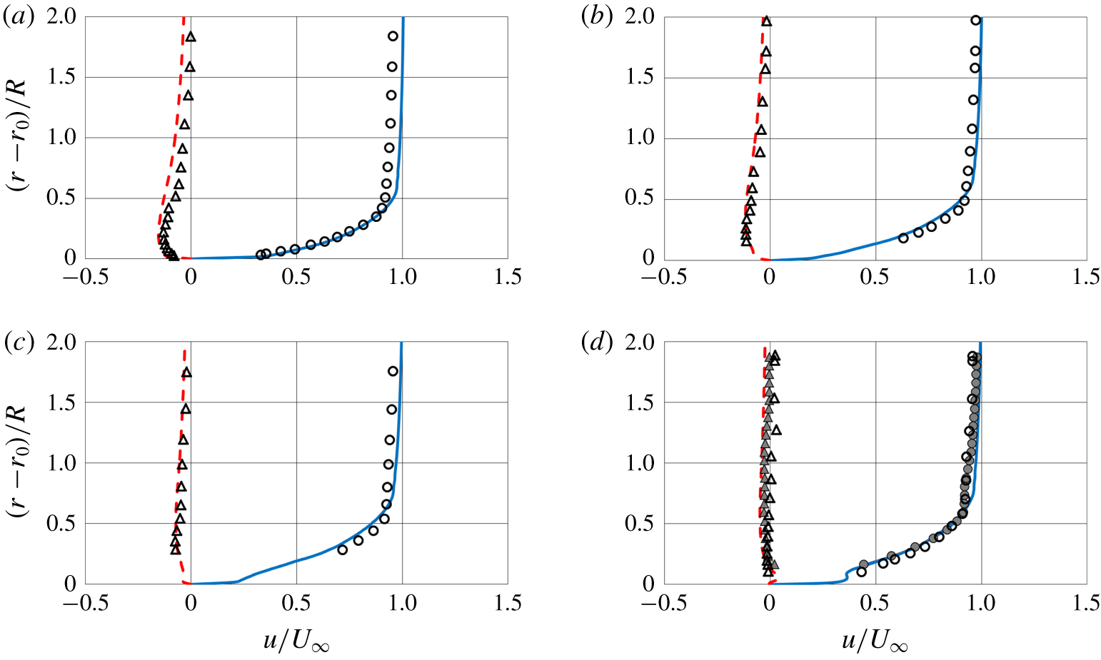
Time-averaged streamwise (solid lines) and radial (dashed lines) velocity profiles from the present simulation at  $Re_{L}=12\times 10^{6}$ at streamwise locations corresponding to
 $x/L=0.904$ (a),
 $x/L=0.927$ (b),
 $x/L=0.956$ (c) and
 $x/L=0.978$ (d). Results from computations extracted over the plane between the fins on the side away from the sail (
 $z=y$ and
 $y>0$). Comparison with measurements on the axial symmetric DSub by Huang et al. (Reference Huang, Liu, Groves, Forlini, Blanton and Gowing1992) (hollow circles and triangles for streamwise and radial velocity, respectively), with the exception of the last location, where experimental measurements on the appended DSub are also shown by solid symbols at the same azimuthal position as LES results. On the vertical axis
 $r_{0}$ stands for the local radial coordinate of the stern surface.

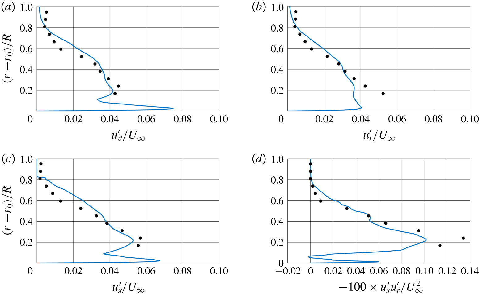
Normal and shear stress distributions at  $Re_{L}=12\times 10^{6}$ on the appended DSub from the present simulation (lines) and measurements by Huang et al. (Reference Huang, Liu, Groves, Forlini, Blanton and Gowing1992) (symbols) at the streamwise location corresponding to
 $x/L=0.978$: (a)
 $u_{\unicode[STIX]{x1D717}}^{\prime }$, (b)
 $u_{r}^{\prime }$, (c)
 $u_{x}^{\prime }$ and (d)
 $-100\times u_{x}^{\prime }u_{r}^{\prime }$. Results extracted over the plane between the fins on the side away from the sail (
 $z=y$ and
 $y>0$).

A direct quantitative comparison on the mean velocity profiles with the measurements by Huang et al. (Reference Huang, Liu, Groves, Forlini, Blanton and Gowing1992) is shown in figure 6. Profiles of streamwise and radial velocity are shown at four stations corresponding to the streamwise locations of the half-chord of the fins ( $x/L=0.904$), immediately downstream of them (
 $x/L=0.927$), half-distance between their trailing edge and the tail of the DSub (
 $x/L=0.956$) and very close to the tail (
 $x/L=0.978$). Note that the measurements were taken on the bare hull, whereas the numerical results were extracted on the meridian plane between the fins on the side away from the sail (
 $z=y$ and
 $y>0$), in order to minimize the influence by the stern appendages, for comparison purposes. An exception is the last location, where experimental results are available also for the appended DSub and are reported by solid symbols at the same azimuthal coordinate as the numerical results. The agreement is very good and the overall development of the boundary layer over the stern is properly captured. At the last station the flow is influenced by the junction vortices from the root of the stern appendages, increasing the momentum in the near-wall region and opposing the effect of the adverse pressure gradient, as shown by the bump in the profile of streamwise velocity. Actually, the influence of the junction vortices is visible also in the measurements by Huang et al. (Reference Huang, Liu, Groves, Forlini, Blanton and Gowing1992), via the comparison between experiments on the DSub with and without stern appendages. They show that, at the selected azimuthal coordinate, the effect of the junction vortices consists of moving streamwise momentum away from the outer layer towards the inner layer and is distinguishable also looking at the increase of the negative radial velocity within the stern boundary layer. For both streamwise and radial velocity components measurements for the appended DSub move indeed closer to the present LES results, compared to the experimental profiles without stern appendages.
In figure 7 the turbulent stresses at  $x/L=0.978$ are compared to the ones from the experiments by Huang et al. (Reference Huang, Liu, Groves, Forlini, Blanton and Gowing1992) on the appended DSub. They were extracted at the same azimuthal coordinate as the mean velocities above. Overall the agreement is satisfactory, especially for the turbulent fluctuations of azimuthal and streamwise velocity components. It is well known that the fluctuations of the normal velocity – which is the radial one at the considered streamwise location – are very challenging to capture. The same behaviour is visible for the profiles of the shear stress. All panels of figure 7 show that the experiments do not have the resolution required to capture the near-wall peak seen in all profiles from the present computations and only display the maximum further out, associated with the internal shear layer.
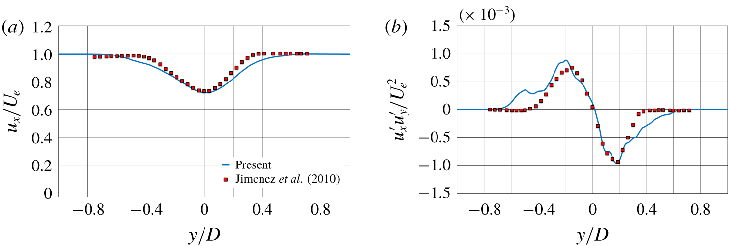
Comparisons at  $Re_{L}=12\times 10^{6}$ with wake measurements by Jiménez et al. (Reference Jiménez, Hultmark and Smits2010a) on the unappended DSub. Location 6 diameters downstream of the tail. Profiles of time-averaged streamwise velocity (a) and
 $u_{x}^{\prime }u_{y}^{\prime }$ shear stress (b) along the
 $y$ direction in the plane of symmetry.
 $U_{e}$ stands for the velocity at the edge of the wake.

For the wake flow, comparisons are presented with the experiments by Jiménez et al. (Reference Jiménez, Hultmark and Smits2010a) at  $Re_{L}=12\times 10^{6}$ on the unappended DSub. We considered those measurements as reference, since results reported for the fully appended DSub by Jiménez et al. (Reference Jiménez, Reynolds and Smits2010b) were taken at much lower values of Reynolds numbers (approximately an order of magnitude). Figure 8 refers to the location six diameters downstream of the tail of the body, along the direction
 $y$ in the plane of symmetry. Figure 8(a) shows that the streamwise velocity at both edges of the wake is slightly lower in the LES profile, which is due to the presence of the stern appendages and the additional momentum deficit in their wake, missing in the wake measurements by Jiménez et al. (Reference Jiménez, Hultmark and Smits2010a) on the bare hull. At inner radii the effect of the wake of the fins is cancelled out by the influence of the junction vortices. They bring higher momentum fluid downstream of the appended DSub, as also reported by Jiménez et al. (Reference Jiménez, Reynolds and Smits2010b), albeit at lower Reynolds numbers. Overall the agreement between computations and experiments in figure 8(a) is good. Comparison for the shear stress,
 $u_{x}^{\prime }u_{y}^{\prime }$, in figure 8(b) is also satisfactory. A dual peak distribution is visible in both LES profiles and measurements, with a good quantitative agreement. At outer radii the wake of the fins is the source of higher values of shear stresses, with an asymmetry caused by the influence of the sail on the side of negative
 $y$ coordinates.
4.2 Analysis of the flow physics
4.2.1 Statistics at the stern boundary layer
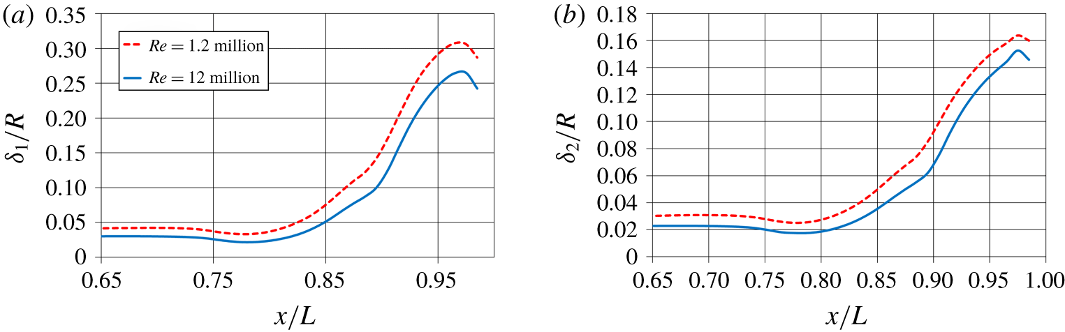
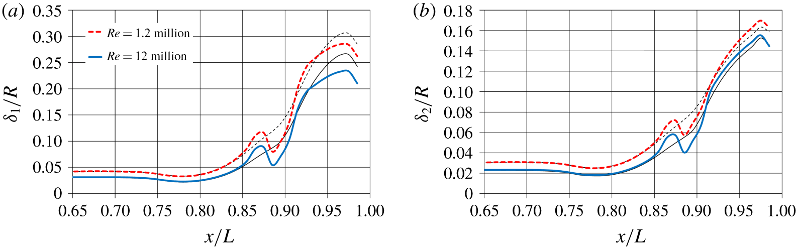
The boundary layer over the cylindrical mid-body is almost a canonical one, whose properties are extensively discussed in the literature, therefore our interest will concentrate towards the stern boundary layer, experiencing a strong adverse pressure gradient and very far from equilibrium conditions. A comparison between Reynolds numbers, concerning the growth of the boundary layer along the stern, is shown in figure 9. The boundary layer thickness is larger for  $Re_{L}=1.2\times 10^{6}$ at all streamwise coordinates and the adverse pressure gradient causes substantial growth in both cases, as demonstrated by the slope of the evolution of
 $\unicode[STIX]{x1D6FF}_{1}$ and
 $\unicode[STIX]{x1D6FF}_{2}$. Note that at the beginning of the stern,
 $x/L\approx 0.75$, the boundary layer thickness experiences actually a slight decrease, since there the convex geometry of the hull produces a mild acceleration of the flow, as shown also by the distributions of pressure and skin-friction coefficients. The most significant boundary layer growth happens in the region
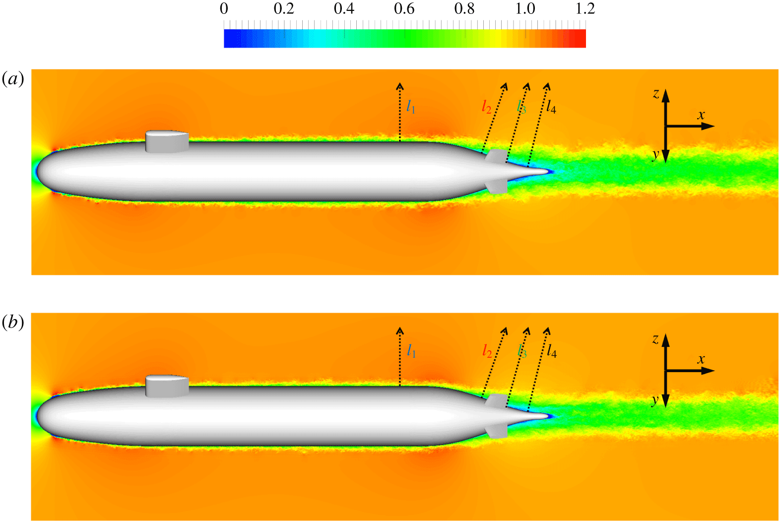
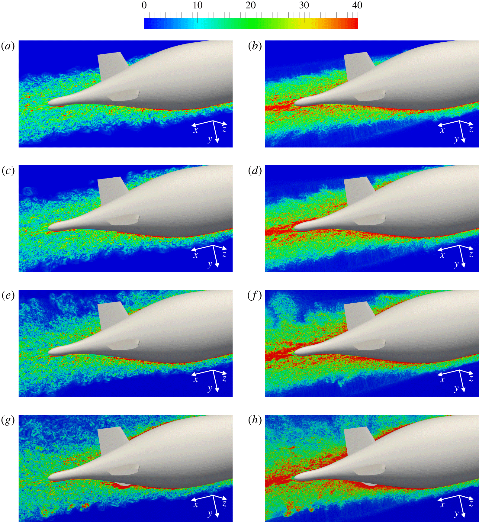
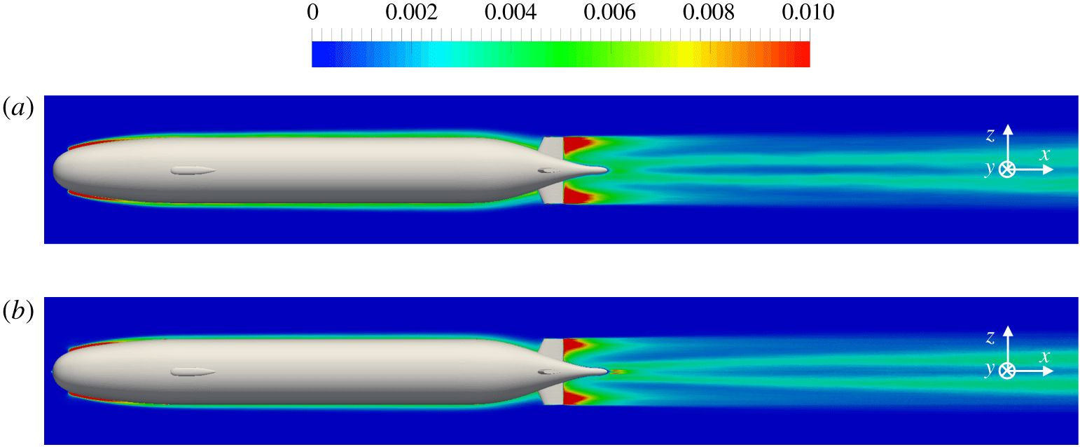
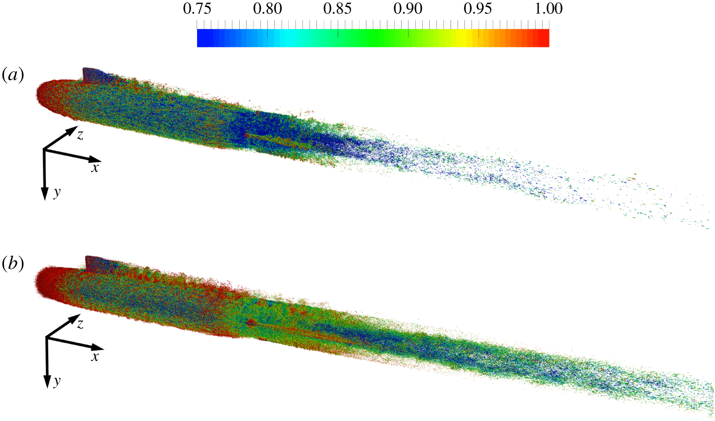
 $0.90<x/L<0.95$, where deceleration is the largest. A global view of the evolution of the boundary layer is shown in figure 10, via instantaneous snapshots of streamwise velocity in the
 $z=y$ plane between the stern appendages. It is clear that: (i) the numerical trip wire triggers a quick transition at the bow; (ii) the boundary layer thickens at the stern, due to the adverse pressure gradient; (iii) the thickness of the boundary layer at the stern sets the width of the wake, which is therefore narrower for
 $Re_{L}=12\times 10^{6}$. However, overall there is a weak dependence of the width of the near wake on the Reynolds number, as also reported in the experimental study by Jiménez et al. (Reference Jiménez, Hultmark and Smits2010a).
Detail of the time-averaged displacement (a) and momentum (b) thickness distributions over the stern. Profiles extracted from the plane between the fins on the side away from the sail ( $z=y$ and
 $y>0$).

Instantaneous streamwise velocity in the plane between the stern appendages ( $z=y$) from the LES computations at
 $Re_{L}=1.2\times 10^{6}$ (Posa & Balaras Reference Posa and Balaras2016a) (a) and
 $Re_{L}=12\times 10^{6}$ (b). Velocity scaled by
 $U_{\infty }$.

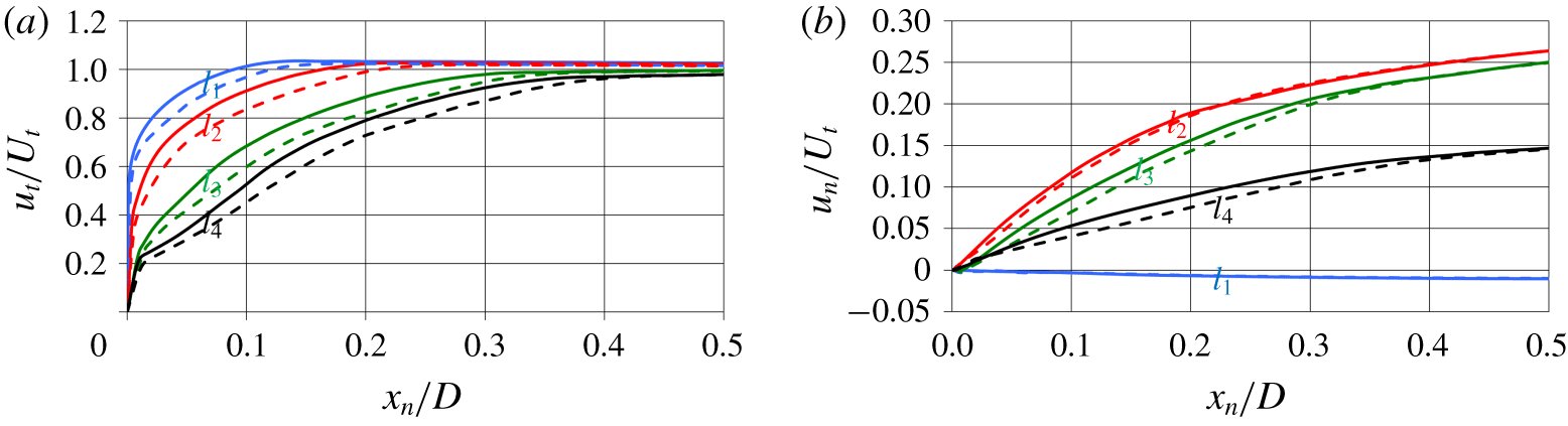
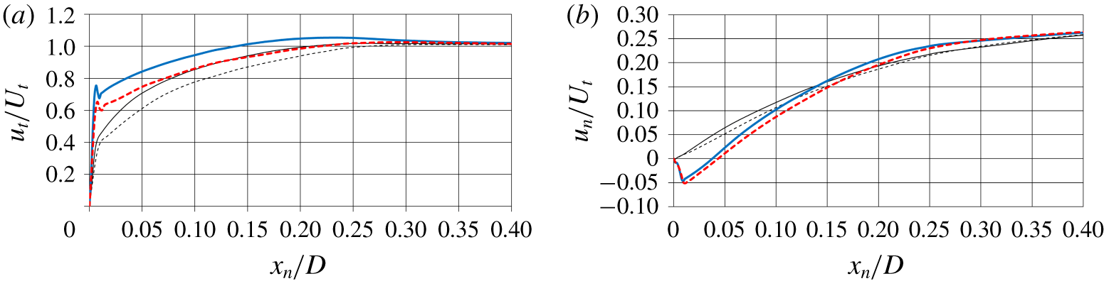
Time-averaged profiles of tangential  $u_{t}$ (a) and normal
 $u_{n}$ (b) velocity along the local direction normal to the stern surface at the streamwise locations
 $l_{1}$ (
 $x/L\approx 0.71$),
 $l_{2}$ (
 $x/L\approx 0.87$),
 $l_{3}$ (
 $x/L\approx 0.92$) and
 $l_{4}$ (
 $x/L\approx 0.96$). Comparison between
 $Re_{L}=1.2\times 10^{6}$ (dashed lines) and
 $Re_{L}=12\times 10^{6}$ (solid lines). Profiles extracted from the plane between the fins on the side away from the sail (
 $z=y$ and
 $y>0$). The variable
 $x_{n}$ stands for the local normal coordinate, while
 $U_{t}$ is the local component of the free-stream velocity tangential to the stern surface.

More details on the evolution of the turbulent boundary layer are reported in figure 11(a), where the time-averaged tangential velocity profiles are shown on the plane between the stern appendages,  $z=y$, on the side opposite to the sail. They were extracted at the streamwise locations
 $x/L\approx 0.71$ (
 $l_{1}$),
 $x/L\approx 0.87$ (
 $l_{2}$),
 $x/L\approx 0.92$ (
 $l_{3}$) and
 $x/L\approx 0.96$ (
 $l_{4}$), which are at the end of the cylindrical mid-body, immediately upstream of the fins, at their trailing edge and downstream of them, respectively, as shown in figure 10. As expected from an equilibrium boundary layer, at
 $l_{1}$ the velocity profile is fuller at the higher Reynolds number, corresponding to smaller values of both displacement and momentum thickness. The shape of the velocity profiles is substantially modified along the stern, featuring a larger size of the outer layer, in comparison with the equilibrium region, due to the strong adverse pressure gradient. Note that at
 $l_{4}$ the velocity profiles experience, in the near-wall region, the additional influence of the junction flows from the appendages, bringing higher momentum in the inner layer. Differences between the two values of Reynolds number are actually more obvious in figure 11(b), where profiles of normal velocity component are reported. At
 $l_{1}$ the normal velocity is negligible. It is slightly negative, because of the mild acceleration at the edge between mid-body and stern. In contrast, at
 $l_{2}$ the normal velocity is a significant fraction of the tangential component: at both Reynolds numbers the boundary layer is growing quickly, with a substantial displacement of momentum away from the stern surface. Values of normal velocity become lower at the locations
 $l_{3}$ and
 $l_{4}$, but they remain quite significant. There, normal velocities are slightly higher at
 $Re_{L}=12\times 10^{6}$, especially in the near-wall region.
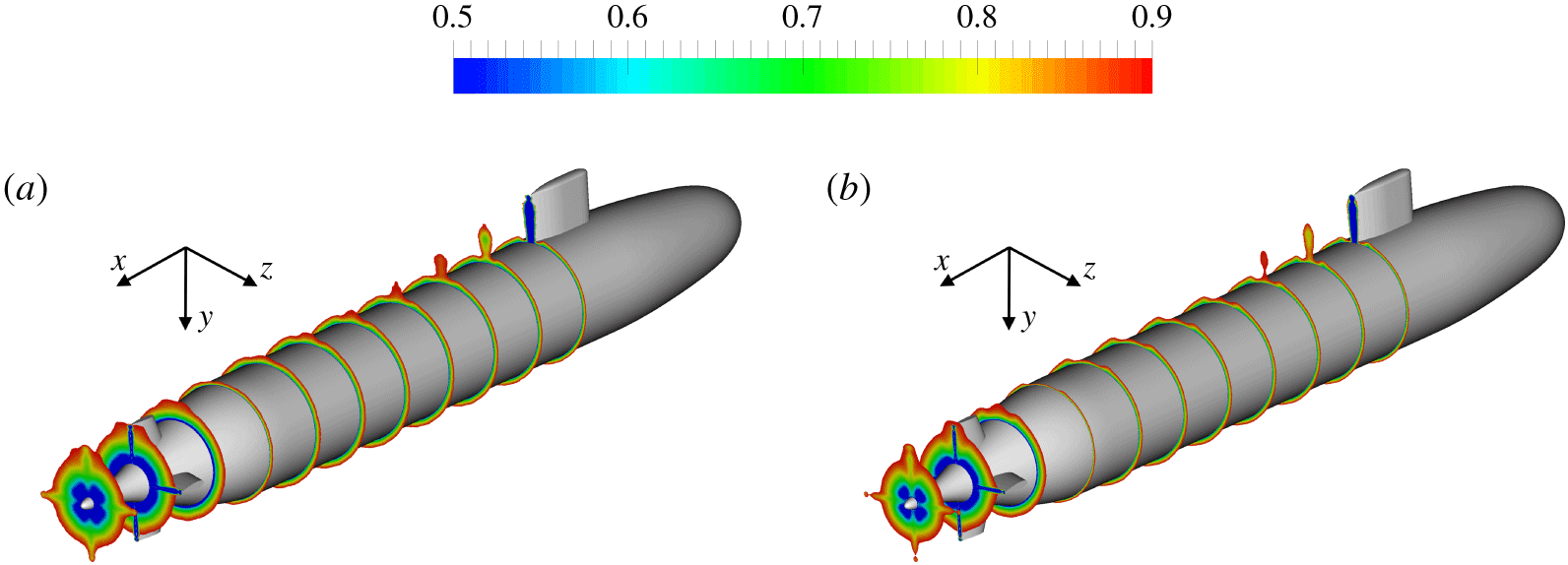
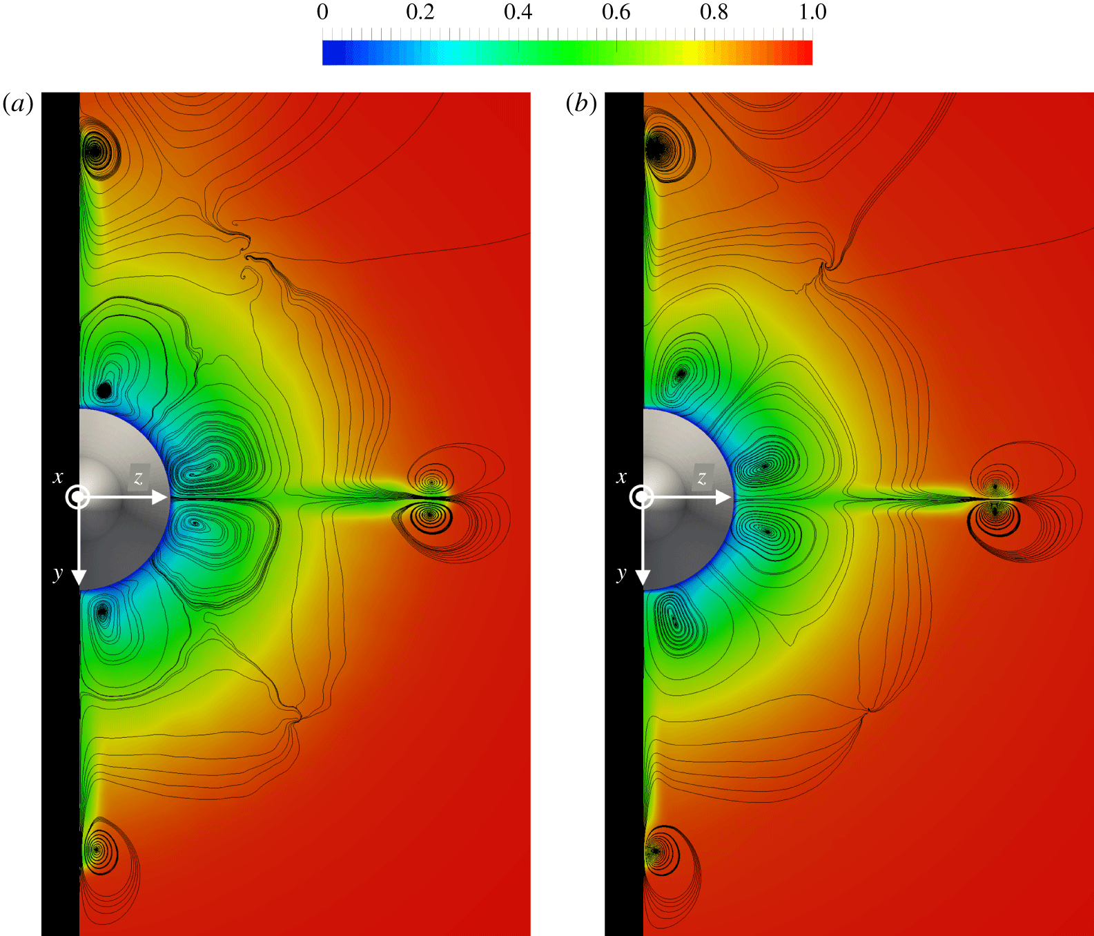
The effect of both adverse pressure gradient across the stern and junction vortices from both sail and fins is well represented in figure 12, where time-averaged contours of streamwise velocity are shown from downstream of the sail up to the tail of the DSub. For visualization purposes, contours were visualized enforcing a maximum threshold equal to  $0.9U_{\infty }$. Results demonstrate for both Reynolds numbers that the junction vortices reorganize the momentum in the wake of both sail and fins, bringing higher momentum into the inner wake of the appendages and lower momentum towards their outer wake. It is also interesting to see that the effect of the junction vortices from the sail remains distinguishable over the whole length of the DSub, up to the fins, where the influence of their junction vortices becomes obviously dominant, producing significant azimuthal gradients, especially at the inner radii of the stern boundary layer. Also in figure 12 it is evident that, at the higher Reynolds number, the boundary layer is thinner, but the growth rate across the rear of the DSub is practically identical between the two considered cases. It is also very obvious at both Reynolds numbers that the boundary layer experiences, between the cylindrical mid-body and the stern, a mild acceleration, reducing locally its thickness.
Time-averaged contours of streamwise velocity from the trailing edge of the sail up to the tail of the DSub. A maximum threshold equal to  $0.9U_{\infty }$ was enforced for visibility purposes. Results at
 $Re_{L}=1.2\times 10^{6}$ (a) and
 $Re_{L}=12\times 10^{6}$ (b).

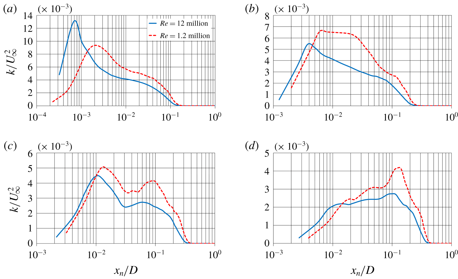
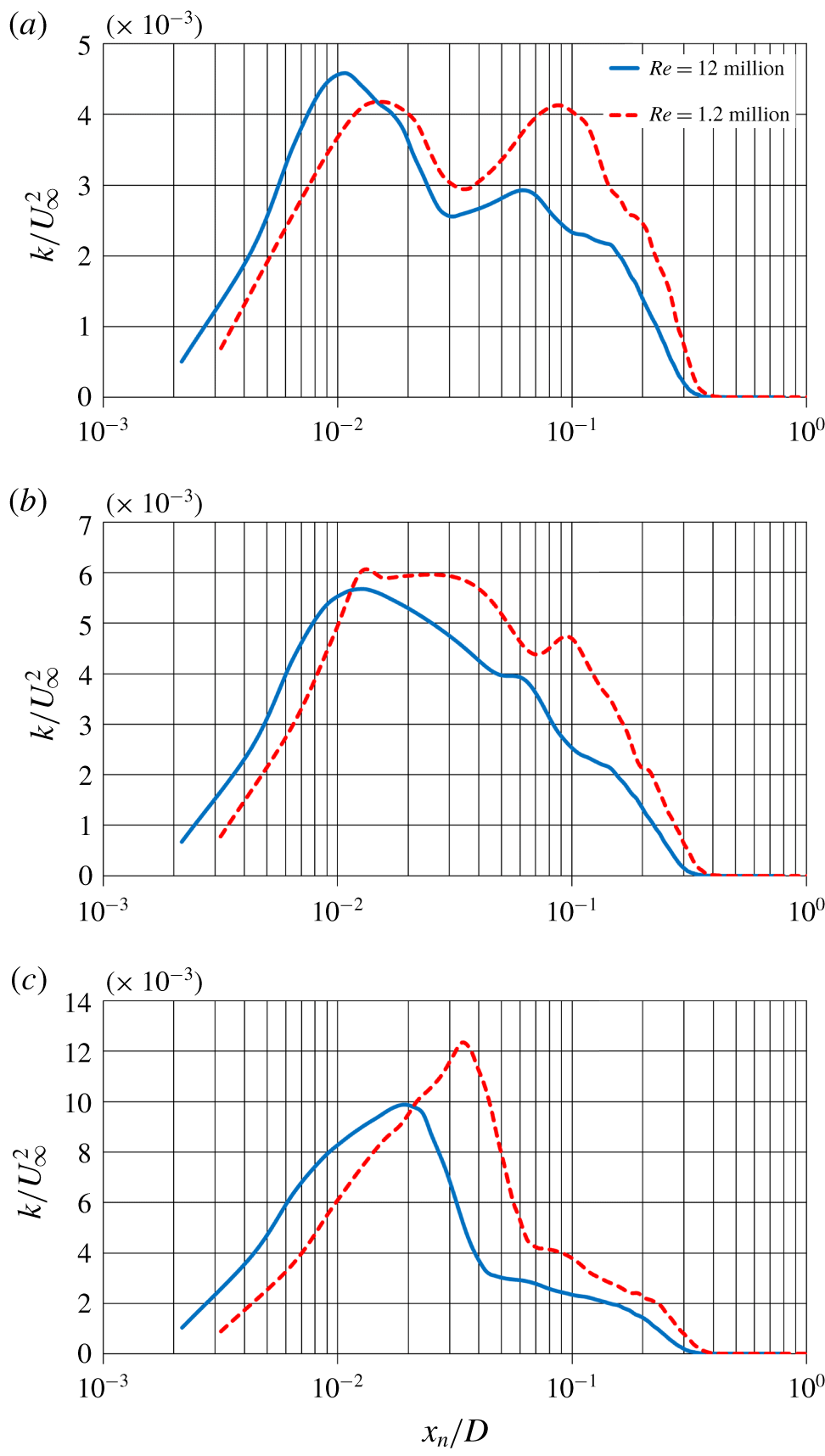
Profiles of turbulent kinetic energy along the local direction normal to the stern surface in the plane between the fins on the side away from the sail ( $z=y$ and
 $y>0$): (a)
 $x/L\approx 0.71$, (b)
 $x/L\approx 0.87$, (c)
 $x/L\approx 0.92$ and (d)
 $x/L\approx 0.96$.

In our earlier work (Posa & Balaras Reference Posa and Balaras2016a) the impact of the adverse pressure gradient on the turbulence distribution was found to be very significant at  $Re_{L}=1.2\times 10^{6}$, affecting also wake features. In that case, we verified that, over the stern, the turbulence peak moves away from the inner layer, towards the outer layer. Such behaviour is actually associated with a decrease of the inner layer turbulence, while outer layer turbulence is almost unaffected. In the present study we observed a similar phenomenon at
 $Re_{L}=12\times 10^{6}$, although the generation of the outer turbulence peak is slower. This is due to lower values of turbulent kinetic energy in the outer layer, as shown in figure 13, where its profiles are represented along the direction normal to the wall again in the plane
 $z=y$ on the side away from the sail. Figure 13(a) refers to the streamwise location at
 $x/L\approx 0.71$ (end of the mid-body). Gradients of turbulent fluctuations between inner and outer layers are more significant at the higher Reynolds number. Values of inner layer turbulence are higher at
 $Re_{L}=12\times 10^{6}$ and vice versa in the outer layer. This is expected, due to the equilibrium nature of the turbulent boundary layer of the mid-body. Figure 13(b) shows the same distributions at the location
 $x/L\approx 0.87$ (upstream of the stern appendages). Values of turbulent kinetic energy in the outer layer are almost unchanged, compared to the upstream location, while the drop of inner layer turbulence is significant, especially at
 $Re_{L}=12\times 10^{6}$. However, turbulence is still higher in the inner layer. The same trend affects the profiles in figure 13(c) for the location
 $x/L\approx 0.92$ (streamwise coordinate of the trailing edge of the fins), but a local outer maximum of turbulent kinetic energy is already distinguishable at both Reynolds numbers. Further downstream in figure 13(d) (
 $x/L\approx 0.96$), the presence of an outer peak is much more obvious at
 $Re_{L}=1.2\times 10^{6}$. Again, outer layer turbulence is almost unaffected, while inner layer turbulence keeps decreasing. As a consequence of this trend, we will show that the bimodal distribution of turbulent fluctuations across the early streamwise development downstream of the DSub is stronger at the lower Reynolds number, because of the larger values of outer layer turbulence within the stern boundary layer, shed into the wake of the body.
4.2.2 Influence of stern appendages on flow features
Flow development along the stern is especially complex. It affects wake features, as extensively discussed in Posa & Balaras (Reference Posa and Balaras2016a), and the flow ingested by the propeller (Posa & Balaras Reference Posa and Balaras2016b, Reference Posa and Balaras2018), although propulsion is not the focus of the present work. Such complexity is tied to the adverse pressure gradient, but also to the presence of appendages and associated wake, tip vortices and junction vortices.
Detail of the time-averaged displacement (a) and momentum (b) thickness distributions over the stern. Profiles extracted from the semi-plane  $\unicode[STIX]{x1D6FF}$ at
 $11^{\circ }$ from the lower fin, whose projection is represented in figure 17. Thinner lines stand for the distributions over the semi-plane
 $\unicode[STIX]{x1D6FC}$ in figure 17, almost unaffected by the junction vortices.

The overall influence of the stern appendages on the development of the boundary layer at the rear of the DSub is shown in figure 14. There, displacement and momentum thicknesses are provided over the meridian semi-plane  $\unicode[STIX]{x1D6FF}$, at
 $11^{\circ }$ from the lower fin, whose projection on a cross-stream section is shown in figure 17 reported below. For comparison, the evolution of the boundary layer thickness over the semi-plane
 $\unicode[STIX]{x1D6FC}$ (see figure 17 for its position) is also reported via thinner lines in the same figure 14 and taken as a reference of a boundary layer almost unaffected by the stern appendages. At the streamwise location corresponding to the leading edge of the fin (
 $x/L\approx 0.88$) for both Reynolds numbers both
 $\unicode[STIX]{x1D6FF}_{1}$ and
 $\unicode[STIX]{x1D6FF}_{2}$ display a couple of local maxima and minima. They are mainly originating from blockage phenomena and the influence of junction vortices there is negligible. The local maximum is indeed tied to lower values of tangential velocity, especially in the outer layer, because of the deceleration upstream of the appendage. Immediately downstream of the leading edge the flow experiences an acceleration, with a consequent sharp decrease of the boundary layer thickness. This is shown in figure 15(a), where the profiles of tangential velocity are provided for both Reynolds numbers over
 $\unicode[STIX]{x1D6FC}$ (thinner lines) and
 $\unicode[STIX]{x1D6FF}$ (thicker lines), demonstrating in the latter case an increase affecting the whole boundary layer thickness. The secondary effect of the junction vortices at this streamwise location, which is limited to the root of the stern appendages, is distinguishable at the inner coordinates, with a small local maximum of tangential velocity very close to the wall and a peak of negative normal velocity in figure 15(b). Thus, higher momentum fluid brought to the inner layer by the junction vortices adds to the decrease of the boundary layer thickness, but in this region of the stern boundary layer this effect is rather marginal and the acceleration near the leading edge of the fins is the main source of the increased tangential velocity. The boundary layer over
 $\unicode[STIX]{x1D6FF}$ accelerates rather uniformly across its whole thickness, with a more obvious increase of tangential velocity for smaller normal coordinates, since the azimuthal distance from the appendage grows moving away from the hull surface. As shown in figure 14, downstream of the leading edge of the fins the gap between distributions over
 $\unicode[STIX]{x1D6FC}$ and
 $\unicode[STIX]{x1D6FF}$ fades out. It grows again downstream of the appendages (
 $x/L>0.92$), due to the influence of the wake of the fin, causing additional momentum deficit. However, moving towards the tail of the DSub, the competing effect of the junction vortices, carrying higher momentum fluid, becomes gradually dominant, because of the momentum recovery within the wake of the fin. This is more evident for the displacement thickness, whose values over
 $\unicode[STIX]{x1D6FF}$ become lower than those over
 $\unicode[STIX]{x1D6FC}$ at the most downstream coordinates of the stern surface. This phenomenon is slightly more distinguishable at the higher Reynolds number, for which also the momentum thickness displays a similar trend very close to the tail.
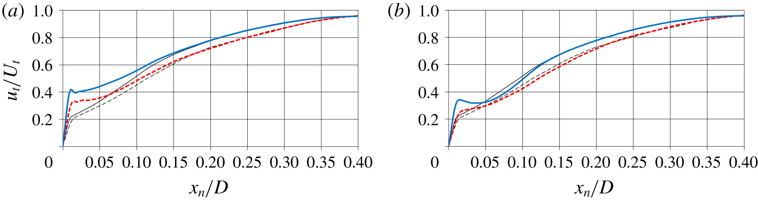
Time-averaged profiles of tangential (a) and normal (b) velocity along the local direction normal to the stern surface at the streamwise location  $x/L=0.885$, immediately downstream of the leading edge of the fins. Thinner and thicker lines stand for the profiles over the semi-planes
 $\unicode[STIX]{x1D6FC}$ and
 $\unicode[STIX]{x1D6FF}$, respectively, represented in figure 17. Comparison between cases at
 $Re_{L}=1.2\times 10^{6}$ (dashed lines) and
 $Re_{L}=12\times 10^{6}$ (solid lines).

The effect of the junction flows on the shape of the boundary layer near the tail is discussed in more detail via figure 16, where time-averaged profiles of tangential velocity are reported at  $x/L\approx 0.96$. In figure 16(a) the profiles over
 $\unicode[STIX]{x1D6FF}$ show an increase of tangential velocity at inner radii, compared to those over
 $\unicode[STIX]{x1D6FC}$, while in the outer region of the boundary layer they practically overlap each other. This behaviour is very similar between the two values of Reynolds number, albeit slightly stronger at
 $Re_{L}=12\times 10^{6}$. Also, at the present streamwise location the influence of the junction vortices extends further away along the azimuthal coordinate. For instance, figure 16(b) shows profiles of tangential velocity over the semi-plane
 $\unicode[STIX]{x1D6FE}$ (see its projection in figure 17 below), located at approximately
 $22^{\circ }$ from the lower fin, where values in the near-wall region differ from those over
 $\unicode[STIX]{x1D6FC}$. Note also that, being the impact of the junction vortices on velocity profiles limited to small normal coordinates, they affect the evolution of the displacement thickness more than that of the momentum thickness, as demonstrated in figure 14. Overall, figure 14 highlights that the growth of the boundary layer thickness is independent of Reynolds number for streamwise locations downstream of the cylindrical section of the DSub, revealing that it is dominated by the effect of the adverse pressure gradient and that the influence of the appendages, via blockage and root vortices, albeit very significant, is practically the same for the two simulated Reynolds numbers, at least within the stern boundary layer. We will show later that differences between the two cases will become more significant in the near wake of the DSub.
Time-averaged profiles of tangential velocity along the local direction normal to the stern surface at the streamwise location  $x/L=0.96$. In panels (a,b) thicker lines stand respectively for the profiles over the semi-planes
 $\unicode[STIX]{x1D6FF}$ and
 $\unicode[STIX]{x1D6FE}$, represented in figure 17. Thinner lines show the profiles over the semi-plane
 $\unicode[STIX]{x1D6FC}$. Comparison between cases at
 $Re_{L}=1.2\times 10^{6}$ (dashed lines) and
 $Re_{L}=12\times 10^{6}$ (solid lines).

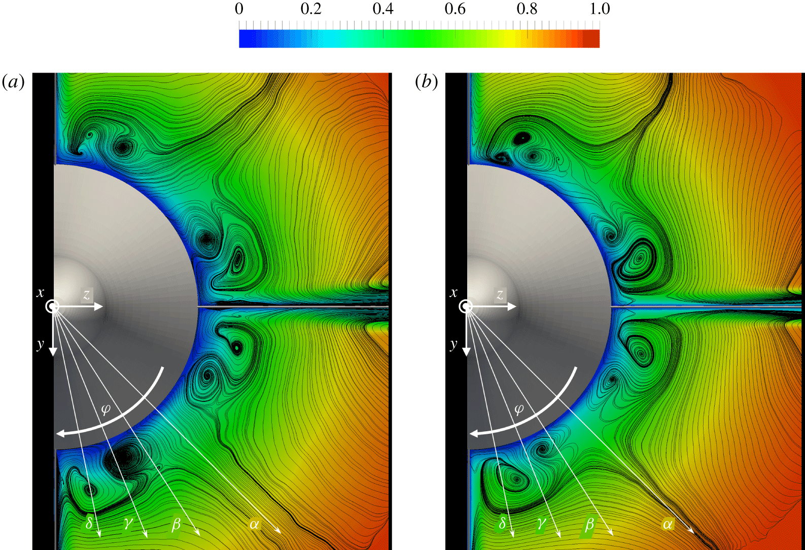
Contours of time-averaged streamwise velocity on the cross-section at the trailing edge of the stern appendages for  $Re_{L}=1.2\times 10^{6}$ (a) and
 $Re_{L}=12\times 10^{6}$ (b). Also the projection of the streamlines of the secondary flows is shown, to emphasize the presence of junction vortices. Velocity scaled by
 $U_{\infty }$.

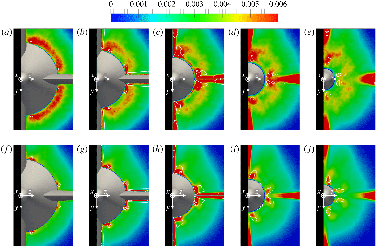
Contours of turbulent kinetic energy on the cross-sections at  $x/L\approx 0.88$ (a,f),
 $x/L\approx 0.90$ (b,g),
 $x/L\approx 0.92$ (c,h),
 $x/L\approx 0.94$ (d,i) and
 $x/L\approx 0.96$ (e,j) for
 $Re_{L}=1.2\times 10^{6}$ (a–e) and
 $Re_{L}=12\times 10^{6}$ (f–j). Values scaled using
 $U_{\infty }^{2}$. Also isolines of the second invariant of the velocity gradient tensor are shown to indicate the areas of highest rotation within the flow field.

Profiles of turbulent kinetic energy at  $x/L\approx 0.92$ along the local directions normal to the stern surface, represented in figure 17: profiles along
 $\unicode[STIX]{x1D6FD}$ (a),
 $\unicode[STIX]{x1D6FE}$ (b) and
 $\unicode[STIX]{x1D6FF}$ (c). For the profiles along the direction
 $\unicode[STIX]{x1D6FC}$ refer to figure 13(c).

More details on junction vortices are reported in figure 17, via the time-averaged field of streamwise velocity at the root of the fins on a cross-section at the trailing edge of the appendages. Also, the projection of the streamlines of the secondary flows is provided, to highlight the presence of junction vortices. Those streamlines were generated by removing from the velocity field the mean radial velocity across the stern boundary layer, in order to isolate the radial flows due to the junction vortices from those tied to the tapered geometry of the stern. Figure 17 shows that: (i) junction vortices affect substantially the streamlines at the root of the stern appendages; (ii) their size is nearly independent of Reynolds number; (iii) a complex pattern of secondary vortices is visible at both Reynolds numbers; (iv) an asymmetry relative to the horizontal plane is generated in both cases, due to the influence by the wake of the sail; (v) the core of the junction vortices is closer to the stern surface at the higher Reynolds number; since the junction vortices originate from the interaction of the stern boundary layer with the leading edge of the stern appendages, it is likely that the thinner boundary layer at  $Re_{L}=12\times 10^{6}$ leads to junction flows closer to the stern surface.
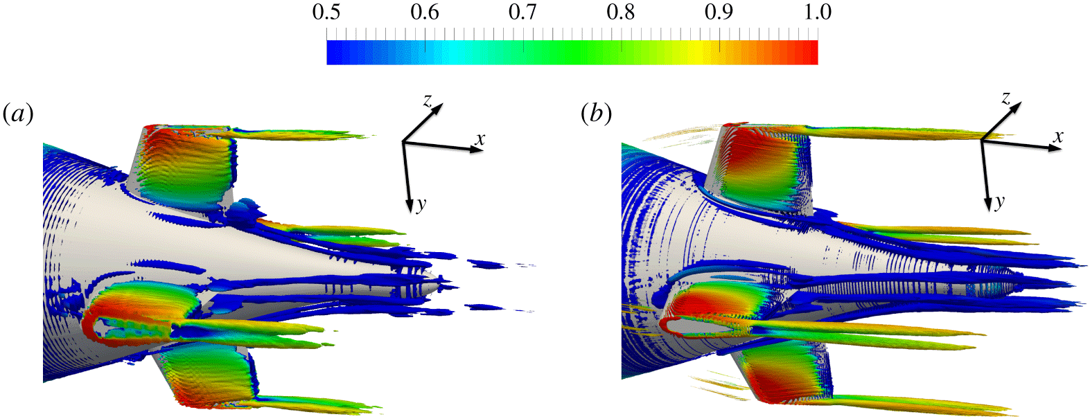
Isosurfaces of  $Q$ (
 $QD^{2}/U_{\infty }^{2}=1$), coloured by streamwise velocity, from the time-averaged fields for
 $Re_{L}=1.2\times 10^{6}$ (a) and
 $Re_{L}=12\times 10^{6}$ (b). Velocity scaled by
 $U_{\infty }$.

Isolines of the second invariant of the velocity gradient tensor,  $Q$, computed from the time-averaged flow fields, are shown in figure 18 at five cross-sections across the stern, to identify the cores of the junction vortices. They are reported on top of contours of turbulent kinetic energy. The impact of the junction vortices on turbulence at the root of the appendages is obvious and is rather similar between the two Reynolds numbers, at least in a qualitative sense. It is also interesting to see that the size of the areas of large rotation of the flow grows up to the trailing edge of the fins, at the streamwise location of panels (c,h), and then it starts decreasing, suggesting that the interaction of the junction vortices with the boundary layer over the appendages plays a role in their enhancement as they move downstream.
Instantaneous contours of vorticity magnitude for  $Re_{L}=1.2\times 10^{6}$ (a,c,e,g) and
 $Re_{L}=12\times 10^{6}$ (b,d,f,h) on the meridian planes
 $\unicode[STIX]{x1D6FC}$ (a,b),
 $\unicode[STIX]{x1D6FD}$ (c,d),
 $\unicode[STIX]{x1D6FE}$ (e,f) and
 $\unicode[STIX]{x1D6FF}$ (g,h). Detail over the stern. Values scaled by
 $U_{\infty }/D$.

Contours of time-averaged streamwise velocity component on the cross-section at  $x/L\approx 0.94$ for
 $Re_{L}=1.2\times 10^{6}$ (a) and
 $Re_{L}=12\times 10^{6}$ (b). Also the projection of the streamlines of the secondary flows is shown, to emphasize the presence of tip and junction vortices. Velocity scaled by
 $U_{\infty }$.

Overall, figure 18 confirms that the influence of Reynolds number on junction vortices is not dramatic in a qualitative sense. However, a more quantitative comparison allows us to provide a better insight into such influence. Values of circulation,  $\unicode[STIX]{x1D6E4}$, were computed via integration of the streamwise vorticity across the areas defined by the isolines in figure 18 at the root of the stern appendages. We excluded from the integration the areas of large
 $Q$ associated with secondary radial flows over the surface of the appendages and in their wake, due to phenomena different from junction vortices (radial pressure gradients across the span of the fins). Values of circulation are reported in table 1. They are obviously larger at the higher Reynolds number. In both cases the evolution is non-monotonic, as suggested by the visualizations in figure 18, since they start decreasing downstream of the fins. Having verified that the effect of the junction vortices on statistics within the stern boundary layer is weakly dependent on Reynolds number, we can conjecture that a lower viscosity allows the generation of stronger junction vortices, but also reduces the propagation of their effect on the surrounding fluid within the stern boundary layer.
Circulation associated with the junction vortices found in figure 18, scaled by  $DU_{\infty }$.

The effect of the junction vortices on turbulence distribution is shown in figure 19, where the profiles of turbulent kinetic energy along the normal to the stern surface are provided at the same streamwise position as in figure 17. They refer to the directions  $\unicode[STIX]{x1D6FD}$,
 $\unicode[STIX]{x1D6FE}$ and
 $\unicode[STIX]{x1D6FF}$ represented in figure 17, while those along the direction
 $\unicode[STIX]{x1D6FC}$ were already reported above in figure 13(c). In figure 19(a) profiles along the direction
 $\unicode[STIX]{x1D6FD}$ are very similar to those along
 $\unicode[STIX]{x1D6FC}$, but junction vortices affect substantially turbulence distribution along the direction
 $\unicode[STIX]{x1D6FE}$ in figure 19(b). In the near-wall region turbulence is higher than away from the appendage, along the directions
 $\unicode[STIX]{x1D6FC}$ and
 $\unicode[STIX]{x1D6FD}$, and an outer peak is not distinguishable at all for
 $Re_{L}=12\times 10^{6}$. Along
 $\unicode[STIX]{x1D6FF}$ (figure 19c) the footprint of the junction vortices is even more evident. Although the inner peak of turbulent kinetic energy is higher at the lower Reynolds number, near wall turbulence is again higher at
 $Re_{L}=12\times 10^{6}$, whereas away from the wall the opposite occurs. The overall influence of the junction vortices on turbulence distribution across azimuthal coordinates is similar at the two Reynolds numbers, although it is felt closer to the wall at
 $Re_{L}=12\times 10^{6}$.
A visualization of the junction vortices is provided via isosurfaces of  $Q$ in figure 20, where also the presence of the tip vortices is very evident. Figure 20 is consistent with the results presented above: (i) the junction vortices originating at the leading edge of the stern appendages induce secondary vortices at closer azimuthal locations, eventually becoming the main vortices downstream; (ii) the junction vortices become stronger at the trailing edge of the fins, where the maximum value of circulation was observed at both Reynolds numbers; (iii) junction vortices are stronger at the higher Reynolds number, for which circulation was indeed found higher; (iv) the roll up between the two sides of each appendage and their tip generates well-distinguishable tip vortices.
Figure 21 displays instantaneous fields of vorticity magnitude at the rear of the DSub, providing a global overview of the evolution of the stern boundary layer. The meridian planes corresponding to the directions  $\unicode[STIX]{x1D6FC}$,
 $\unicode[STIX]{x1D6FD}$,
 $\unicode[STIX]{x1D6FE}$ and
 $\unicode[STIX]{x1D6FF}$ are considered. In agreement with the statistics for turbulent kinetic energy, moving closer to the stern appendages, values of vorticity magnitude increase. This phenomenon is mainly due to the boundary layer over the fins and junction flows, thus it is already distinguishable in the region between the fins, affecting also the locations downstream of them. Over the planes
 $\unicode[STIX]{x1D6FE}$ and
 $\unicode[STIX]{x1D6FF}$, the closest to the plane of symmetry of the DSub, vorticity is higher on the upper side of each panel, due to the additional structures populating the wake of the sail. The above behaviours are similar between the two Reynolds numbers, although vorticity magnitude is higher at
 $Re_{L}=12\times 10^{6}$, with also higher values at the axis of the overall wake generated by the DSub. The size of the structures is obviously larger at
 $Re_{L}=1.2\times 10^{6}$, with the finer computational grid adopted at
 $Re_{L}=12\times 10^{6}$ proving to be able to resolve the smaller scales populating the stern boundary layer.
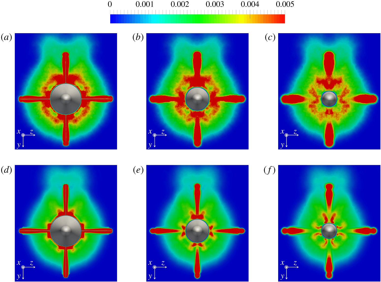
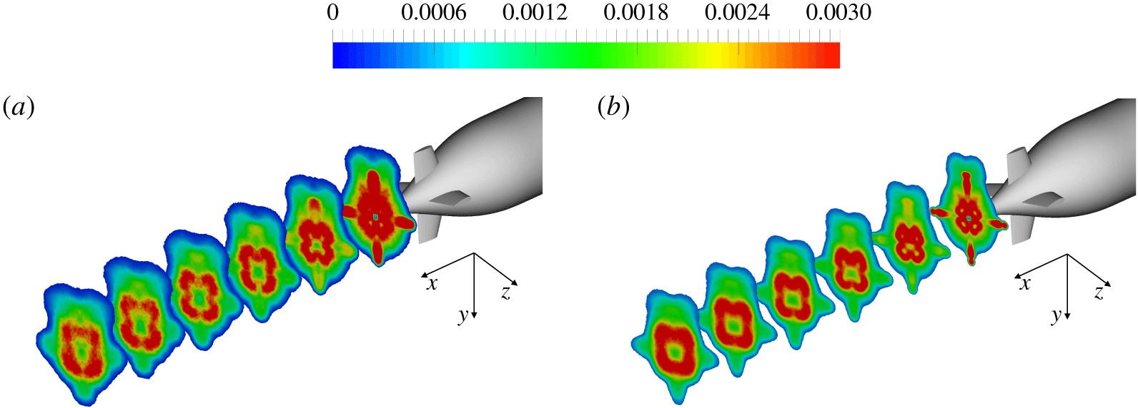
Contours of turbulent kinetic energy for  $Re_{L}=1.2\times 10^{6}$ (a–c) and
 $Re_{L}=12\times 10^{6}$ (d–f). Streamwise locations corresponding to
 $x/L\approx 0.92$ (a,d),
 $x/L\approx 0.94$ (b,e) and
 $x/L\approx 0.96$ (c,f). Values scaled by
 $U_{\infty }^{2}$.

The footprint of the junction vortices downstream of the stern appendages is shown in figure 22 for both Reynolds numbers at a location  $x/L\approx 0.94$ in the wake of the fins. Also the presence of tip vortices is visible. They originate from the pressure gradient between the tip and the lateral surfaces of the fins, even at the 0 yaw angle considered in our computations. Again, asymmetries relative to the horizontal plane are due to the influence by the wake of the sail on the upper side. Compared to the upstream location considered above, the pattern in figure 22 is less complex, without significant secondary vortices associated with the primary junction vortices.
Junction vortices keep affecting turbulent kinetic energy fields in the wake of the appendages. In figure 23 locations corresponding to  $x/L\approx 0.92$ (a,d),
 $x/L\approx 0.94$ (b,e) and
 $x/L\approx 0.96$ (c,f) are considered for both Reynolds numbers. In both cases junction vortices cause higher values of turbulent kinetic energy at the root of the fins, feeding additional turbulence into the stern boundary layer. In addition, downstream of the appendages, values of turbulent kinetic energy away from the wall are higher at the lower Reynolds number. The turbulence outer peak, coming from the stern boundary layer, is easily distinguishable for
 $Re_{L}=1.2\times 10^{6}$, whereas this is not the case at
 $Re_{L}=12\times 10^{6}$. This makes the role of the junction vortices in turbulence shed in the wake by the DSub relatively more significant at the higher Reynolds number. Also the wake of the sail affects turbulence fields: higher values of turbulent kinetic energy populate the upper region of each field for both Reynolds numbers. The comparison between Reynolds numbers highlights that also turbulence associated with the wake of the sail is higher at
 $Re_{L}=1.2\times 10^{6}$. Values are very high downstream of the fins. As expected, the width of their wake is larger at the lower Reynolds number. Note that such turbulence fades away quickly, keeping higher values at outer radii, due to the tip vortices originating from the stern appendages.
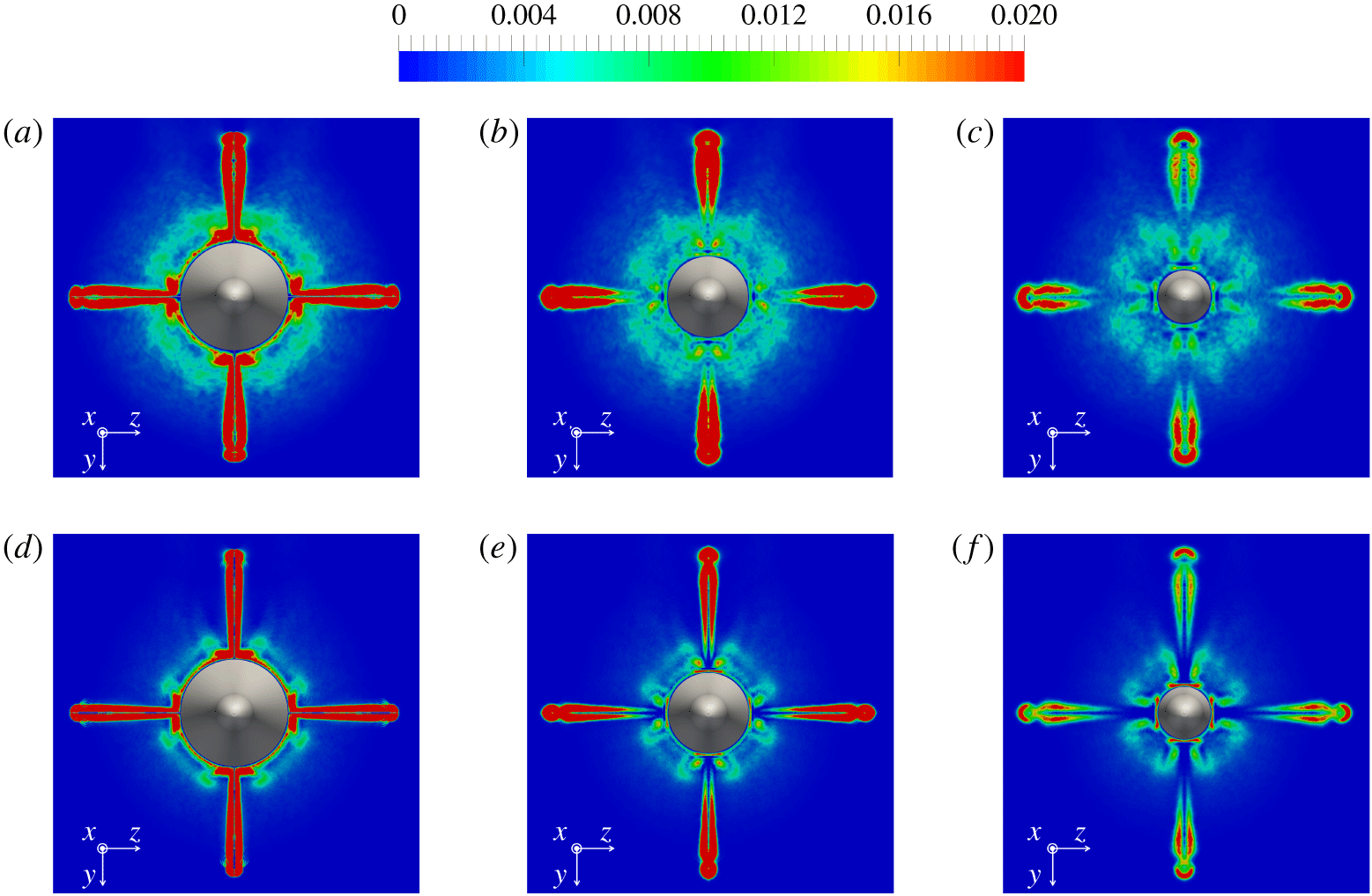
Contours of production of turbulent kinetic energy for  $Re_{L}=1.2\times 10^{6}$ (a–c) and
 $Re_{L}=12\times 10^{6}$ (d–f). Streamwise locations corresponding to
 $x/L\approx 0.92$ (a,d),
 $x/L\approx 0.94$ (b,e) and
 $x/L\approx 0.96$ (c,f). Values scaled by
 $U_{\infty }^{3}/D$.

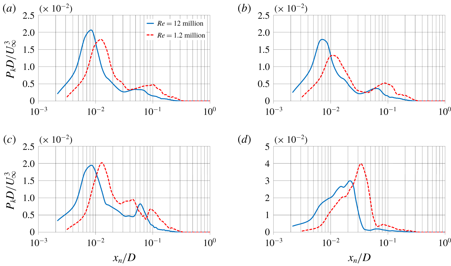
Similarities between the computations carried out at the two Reynolds numbers are evident also in figure 24, where contours for the production of turbulent kinetic energy are shown. It is interesting to notice the complex pattern downstream of the root of the fins. Junction vortices enhance substantially the overall production, which is instead much smaller within the stern boundary layer, due to the dramatic reduction of the gradients over the rear of the DSub. This causes a drastic decrease of production, compared to that within an equilibrium boundary layer. Also in this case the role of the junction vortices is relatively more significant at the higher Reynolds number. As we are going to show, although production in the core of the junction vortices is slightly higher at  $Re_{L}=1.2\times 10^{6}$, its contribution to overall production, relative to that in the stern boundary layer, is more significant at
 $Re_{L}=12\times 10^{6}$. Also in figure 24 we can see that the footprint of the wake of the fins, which is very evident in all panels, displays a more dramatic decreasing trend, in comparison with that at the inner radii, affected by the junction vortices. Moreover, in figure 24 the influence of the sail is weak. However, at both Reynolds numbers slightly higher values are visible at inner radii on the side of the sail, with instead lower values at outer radii. This is consistent with the results by Jiménez et al. (Reference Jiménez, Reynolds and Smits2010b), who reported a destructive effect by the wake of the sail on the shear stresses in the wake of the DSub, where they were slightly higher on the side opposite to the sail.
Profiles of production of turbulent kinetic energy at  $x/L\approx 0.92$ along the local directions normal to the stern surface, represented in figure 17: profiles along
 $\unicode[STIX]{x1D6FC}$ (a),
 $\unicode[STIX]{x1D6FD}$ (b),
 $\unicode[STIX]{x1D6FE}$ (c) and
 $\unicode[STIX]{x1D6FF}$ (d).

A more quantitative comparison is presented in figure 25, where the four panels show the profiles of production of turbulent kinetic energy along the directions  $\unicode[STIX]{x1D6FC}$,
 $\unicode[STIX]{x1D6FD}$,
 $\unicode[STIX]{x1D6FE}$ and
 $\unicode[STIX]{x1D6FF}$, already defined in figure 17, at the streamwise location
 $x/L\approx 0.92$. It is worth noting that, away from the fins, the peak of production of turbulent kinetic energy remains in the inner layer, which is still the region with the largest velocity gradients, although a second lower peak is generated in the outer layer. Production in the near-wall region is higher at
 $Re_{L}=12\times 10^{6}$, whereas the opposite occurs away from the wall, consistent with the behaviour seen for the turbulent kinetic energy. Production experiences an increase in the vicinity of the lower fin. This is already visible in the outer region of the stern boundary layer along the direction
 $\unicode[STIX]{x1D6FE}$ in panel (c), where production is enhanced, compared to that in panels (a,b). However, the effect of the junction flows becomes more evident along
 $\unicode[STIX]{x1D6FF}$ in panel (d), with again higher values near the wall at the higher Reynolds number and away from the wall at the lower Reynolds number, since junction vortices keep closer to the stern surface in the former case. It is also interesting to notice from figure 25(d) that, for both Reynolds numbers, the near-wall trend is actually the result of the overlap of multiple local maxima, as also shown in figure 24.
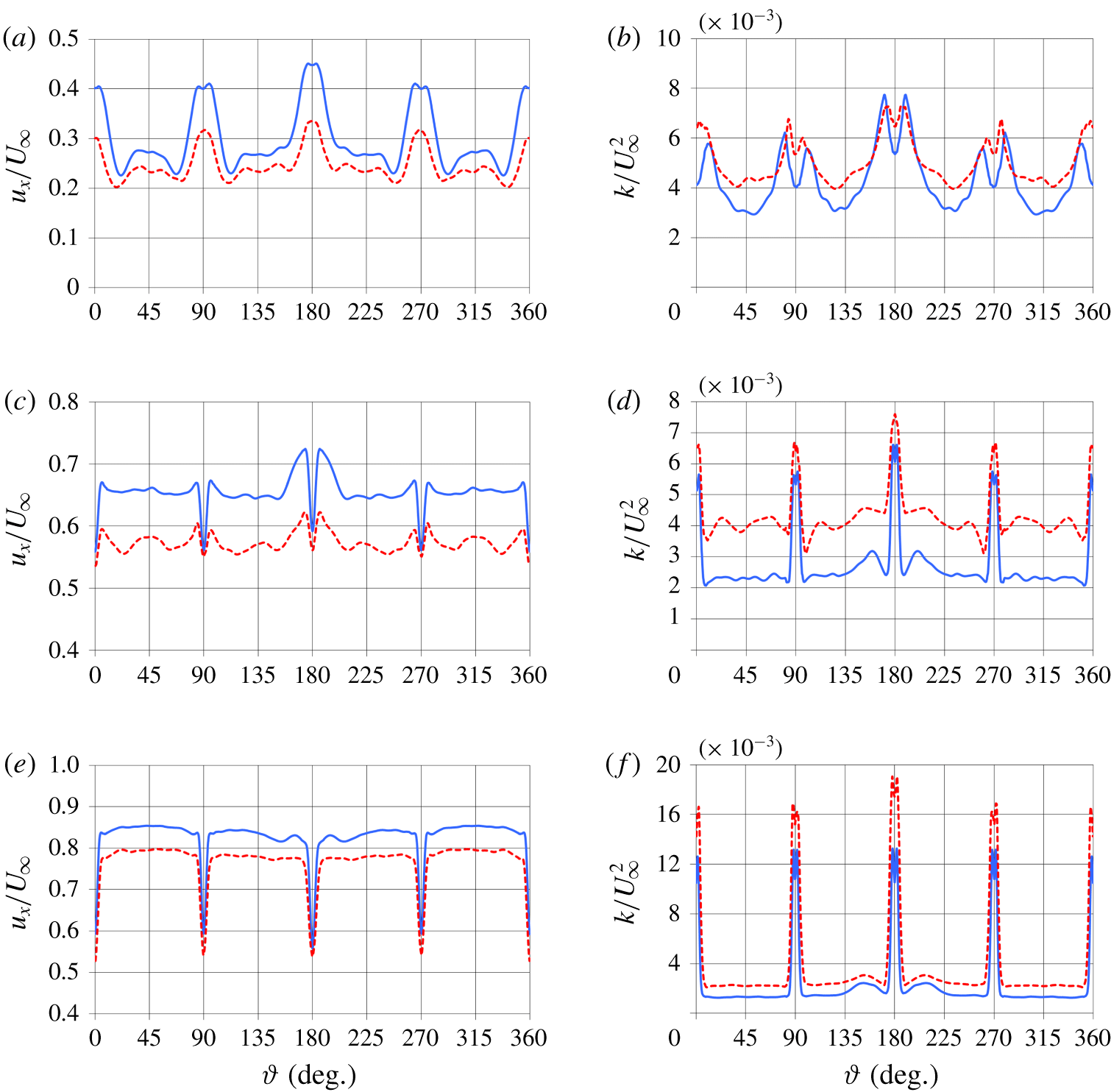
Azimuthal profiles of streamwise velocity (a,c,e) and turbulent kinetic energy (b,d,f) for  $Re_{L}=1.2\times 10^{6}$ (dashed lines) and
 $Re_{L}=12\times 10^{6}$ (solid lines) at the streamwise location
 $x/L\approx 0.94$. Distributions at
 $r/D=0.15$ (a,b),
 $r/D=0.25$ (c,d) and
 $r/D=0.35$ (e,f).

The contours above highlight that the impact of the junction vortices on first-order and second-order statistics within the stern boundary layer is not substantially dependent on Reynolds number, at least for a change of an order of magnitude, as in the present case. This is demonstrated more quantitatively by figure 26, where azimuthal profiles of streamwise velocity component (left) and turbulent kinetic energy (right) are shown at  $x/L\approx 0.94$. Results at additional streamwise locations between the fins and downstream of them were not reported here due to limitation of space, but we verified that they agree with the conclusions below. At the radial coordinate
 $r/D=0.15$ the momentum gain associated with the junction vortices generates maxima of streamwise velocity at the azimuthal coordinates corresponding to the locations of the fins (figure 26a). The low momentum fluid in the wake of the appendages is carried away from those azimuthal locations by the junction vortices, producing this way the local minima seen at both sides of each peak of streamwise velocity. The effect of the junction vortices generated by the sail is very obvious even at the tail of the DSub for both Reynolds numbers, since the maximum at
 $\unicode[STIX]{x1D717}=180^{\circ }$ is significantly higher than those in the wake of the fins not aligned with the sail. The azimuthal extent of the region affected by the junction vortices is similar for the two Reynolds numbers, as well as the momentum gain directly downstream of the fins, relative to the streamwise velocity within the stern boundary layer. This momentum gain is only slightly higher at
 $Re_{L}=12\times 10^{6}$. In figure 26(b) values of turbulent kinetic energy at the couples of maxima associated with the junction vortices are very close between Reynolds numbers, in contrast with the lower values of outer layer turbulence for the higher Reynolds number at the azimuthal coordinates away from the fins. Also in the azimuthal distributions of turbulent kinetic energy the footprint of the junction vortices from the sail is still significant, being the source of the higher values observed around
 $\unicode[STIX]{x1D717}=180^{\circ }$. Moving away from the surface of the stern at
 $r/D=0.25$ (figure 26c) the influence of the junction vortices is weaker, but it remains easily distinguishable. Minima of streamwise velocity occur directly downstream of the fins, because of the momentum deficit in their wake, but the maxima at both edges of each wake confirm the significant role of the junction vortices in readjusting the distribution of momentum downstream of the appendages. Also at this radial location such influence is not obviously dependent on the Reynolds number, although in this panel it is slightly stronger at
 $Re_{L}=1.2\times 10^{6}$, with the exception of the region aligned with the wake of the sail. In figure 26(d) the highest values of turbulent kinetic energy are associated with the wake of the fins, but local maxima/minima still populate the edge of those wakes. In agreement with the results for the streamwise velocity, except for the area around
 $\unicode[STIX]{x1D717}=180^{\circ }$, the distribution away from the wake of the fins is more uniform at the higher Reynolds number. As discussed above, looking at the normal profiles of turbulent kinetic energy, at
 $Re_{L}=12\times 10^{6}$ the influence of the junction vortices is felt slightly closer to the surface of the stern, thus it fades out more quickly moving away to larger radial coordinates. Further away from the hull surface, at
 $r/D=0.35$ (figure 26e,f), the footprint of the junction vortices from the stern appendages is missing in both momentum and turbulence distributions. Instead, that of the junction vortices from the sail is still a source of small local maxima of streamwise velocity and turbulent kinetic energy at the edges of the wake centred at
 $\unicode[STIX]{x1D717}=180^{\circ }$, although the most evident flow features are obviously the momentum deficit in the wake of the fins and the turbulence peak within the shear layer shed from their trailing edge.
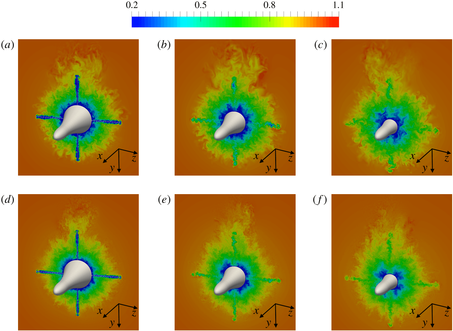
Instantaneous contours of streamwise velocity for  $Re_{L}=1.2\times 10^{6}$ (a–c) and
 $Re_{L}=12\times 10^{6}$ (d–f). Streamwise locations corresponding to
 $x/L\approx 0.92$ (a,d),
 $x/L\approx 0.94$ (b,e) and
 $x/L\approx 0.96$ (c,f). Values scaled by
 $U_{\infty }$.

The increase of momentum directly downstream of the fins in the near-wall region is shown in figure 27, where instantaneous contours of streamwise velocity are reported at the same streamwise locations considered in figure 23. The momentum deficit at inner radii is higher away from the appendages, with azimuthal gradients increasing moving from the left to the right sides of figure 27. The opposite occurs at outer radii, where momentum deficit is higher in the wake of the fins, but the wake recovery across the panels of figure 27 makes the azimuthal distribution of velocity more uniform moving away from the stern appendages. Also, in agreement with the discussion above, although the thickness of the stern boundary layer is slightly dependent on the Reynolds number, its size is dominated by the effect of the adverse pressure gradient. The difference between the two Reynolds number cases is indeed small, compared to the overall boundary layer thickness at the tail of the DSub.
4.2.3 Near-wake development
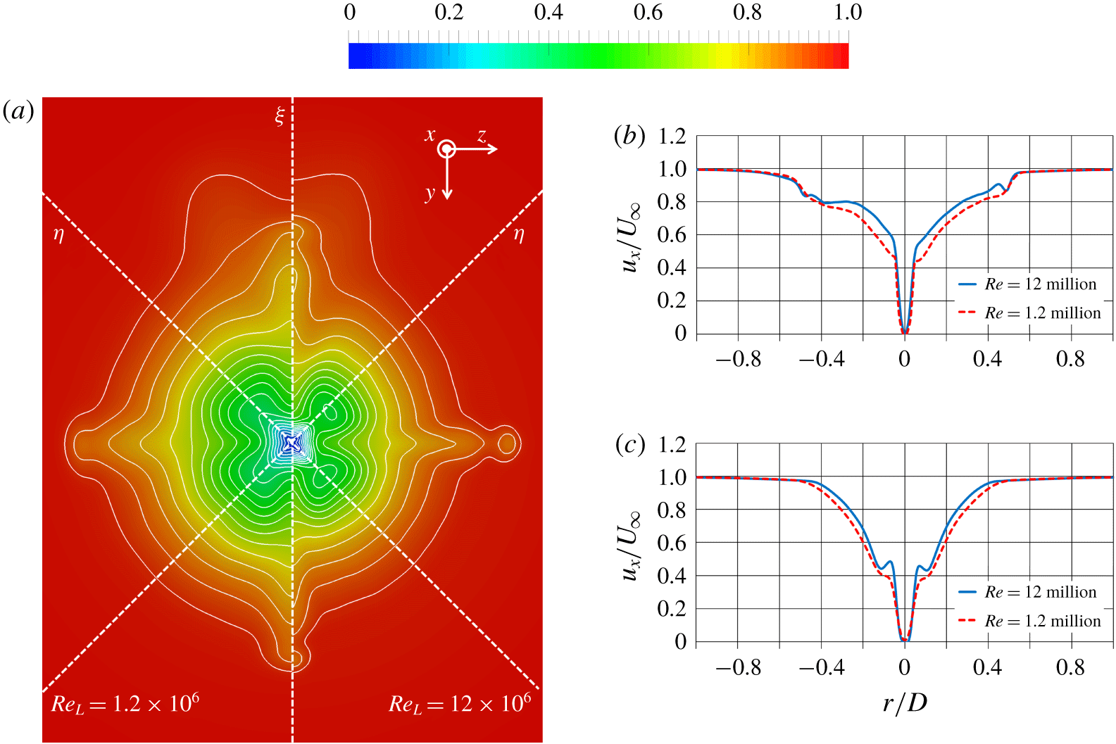
(a) Time-averaged contours of streamwise velocity at the tail of the DSub for  $Re_{L}=1.2\times 10^{6}$ (left) and
 $Re_{L}=12\times 10^{6}$ (right); (b) profiles along the direction
 $\unicode[STIX]{x1D709}$ shown in (a); (c) profiles along the directions
 $\unicode[STIX]{x1D702}$ shown in (a). Velocity scaled by
 $U_{\infty }$.

In this section we will compare the near-wake development for the two simulated Reynolds numbers. Figure 28(a) shows time-averaged contours of streamwise velocity as well as isolines for both  $Re_{L}=1.2\times 10^{6}$ (left) and
 $Re_{L}=12\times 10^{6}$ (right) at the tail of the DSub. With no appendages isolines would be circumferential. Their deformation is caused by the wake of the appendages and by the junction and tip flows originating from them. Inner radii show the effect of the junction vortices. The deformation of the isolines there is due to the higher momentum fluid that junction vortices bring in the wake of the fins, with lower momentum fluid away from them. Such deformation is more evident at
 $Re_{L}=12\times 10^{6}$. Streamwise velocity profiles were extracted along the directions
 $\unicode[STIX]{x1D709}$ and
 $\unicode[STIX]{x1D702}$ and compared between the two Reynolds numbers in figure 28(b) and figure 28(c), respectively. In figure 28(b) the comparison along
 $\unicode[STIX]{x1D709}$ shows: (i) a higher momentum deficit at the lower Reynolds number; (ii) a similar momentum deficit due to tip flows (
 $r/D\approx \pm 0.5$); (iii) a similar footprint of the wake of the sail for the two Reynolds numbers (
 $r/D<-0.5$). Profiles in figure 28(c) along
 $\unicode[STIX]{x1D702}$ are not affected by the wake of the sail and the tip flows from the fins and the effect of the junction vortices from the stern appendages can be isolated. Compared to figure 28(b), momentum deficit at inner radii is higher, which is due to the lower momentum fluid that junction vortices carry away from the wake of the fins, from the azimuthal location
 $\unicode[STIX]{x1D709}$ towards the azimuthal location
 $\unicode[STIX]{x1D702}$. This is especially evident at the higher Reynolds number, with local minima at radial coordinates
 $r/D\approx \pm 0.1$. In contrast, at outer radii momentum deficit is lower, compared to the profiles along
 $\unicode[STIX]{x1D709}$, being
 $\unicode[STIX]{x1D702}$ away from the wake of both sail and fins.
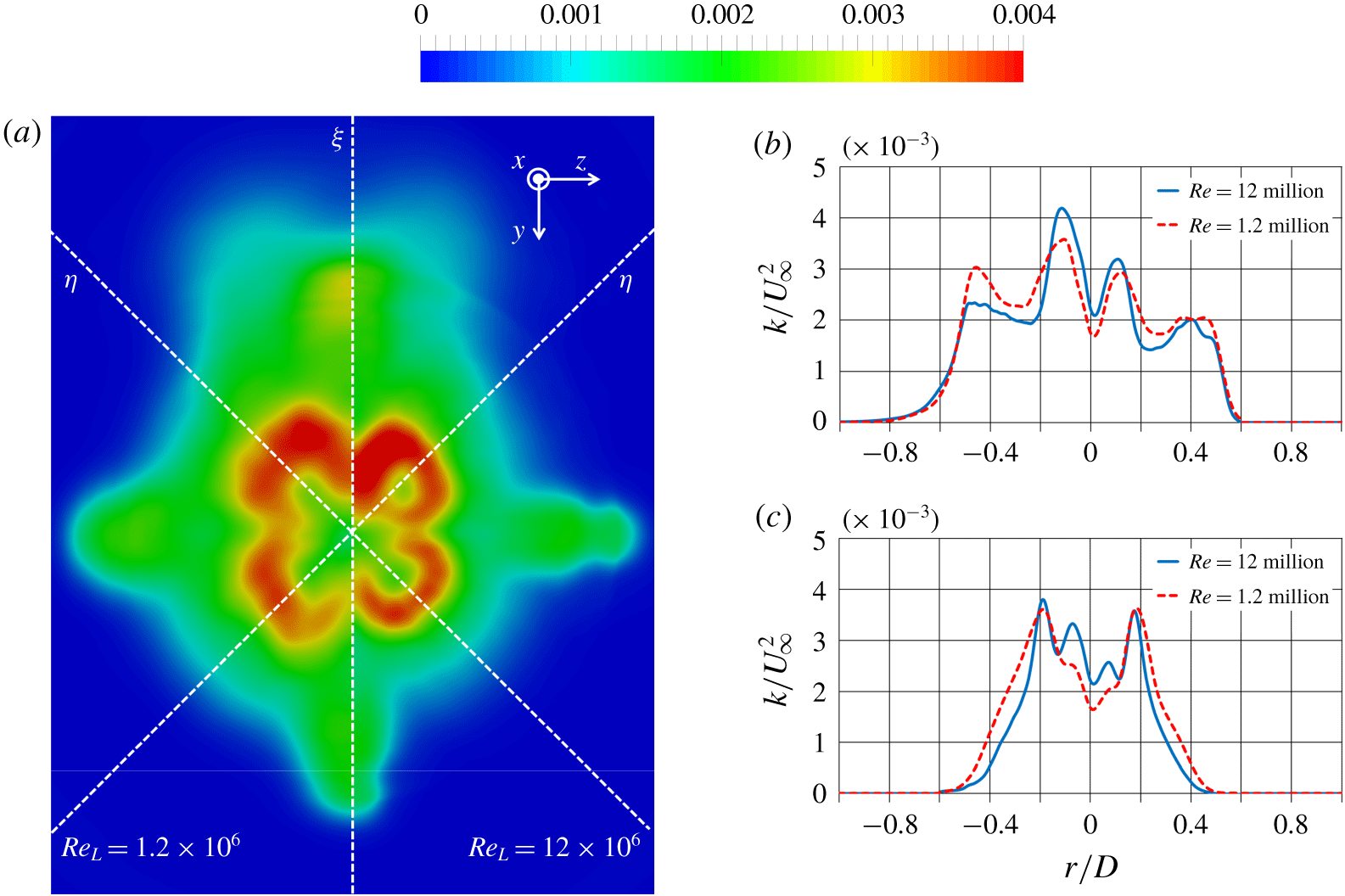
(a) Contours of turbulent kinetic energy at the tail of the DSub for  $Re_{L}=1.2\times 10^{6}$ (left) and
 $Re_{L}=12\times 10^{6}$ (right); (b) profiles along the direction
 $\unicode[STIX]{x1D709}$ shown in (a); (c) profiles along the directions
 $\unicode[STIX]{x1D702}$ shown in (a). Values scaled by
 $U_{\infty }^{2}$.

Results for turbulent kinetic energy at the tail are provided in figure 29. Figure 29(a) shows higher values at outer radii for  $Re_{L}=1.2\times 10^{6}$, which displays a more obvious outer maximum, in agreement with the discussion on boundary layer development in § 4.2.1. We have found, looking at the boundary layer over the stern, that the near-wall turbulence fades away dramatically at both Reynolds numbers and the inner peak is not visible anymore upstream of the tail (see figure 13d). However, due to turbulence associated with junction vortices, in figure 29(a) a local maximum of turbulent kinetic energy is produced at inner radii, even along the directions
 $\unicode[STIX]{x1D702}$, especially at the higher Reynolds number. We recall that the azimuthal extent of the junction vortices, relative to the stern, grows moving downstream, due to the tapered geometry of the aft of the DSub. Therefore they are able to affect also azimuthal coordinates away from the appendages. Figure 29(b) and figure 29(c) allow more quantitative considerations. Profiles along
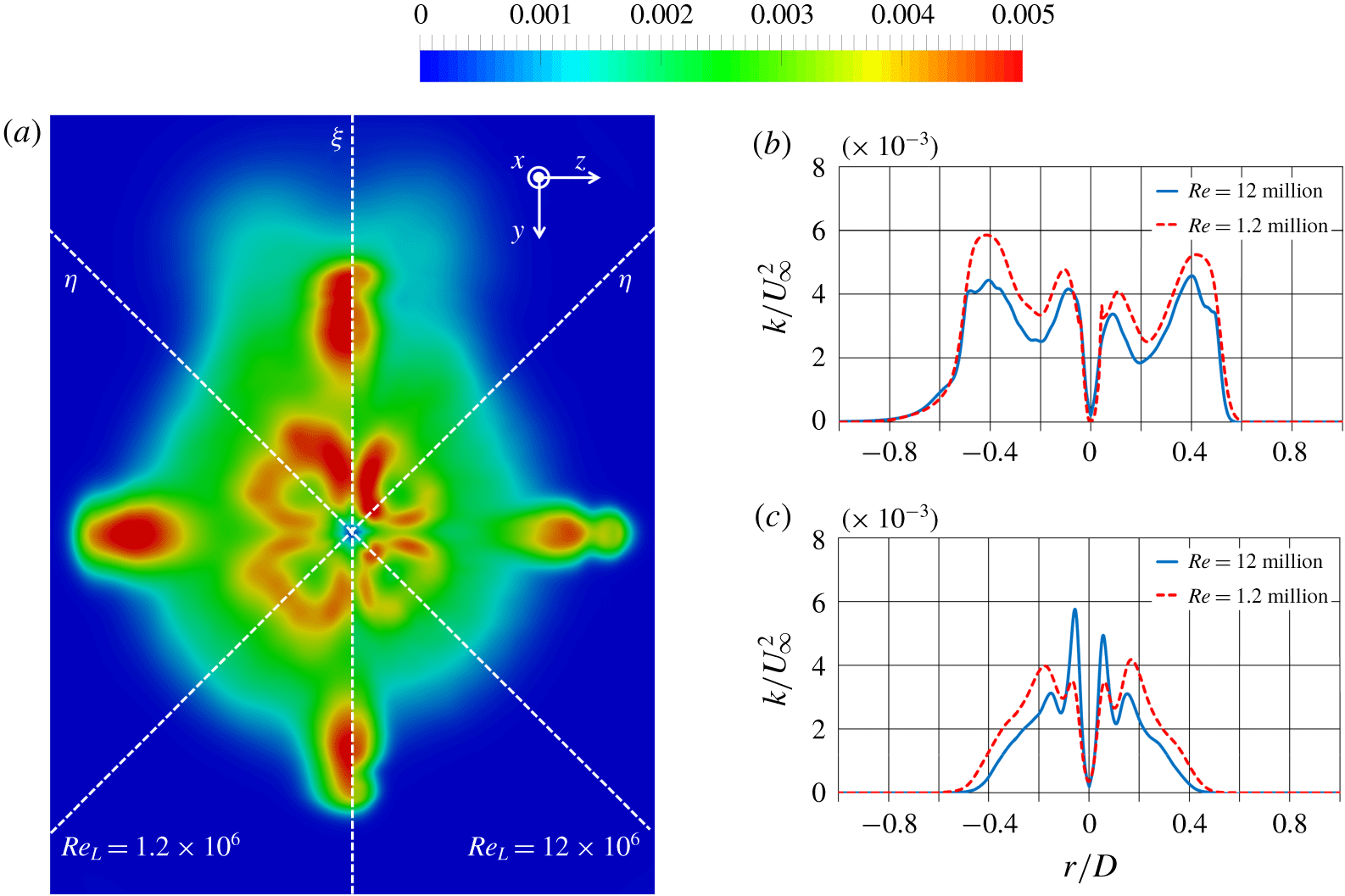
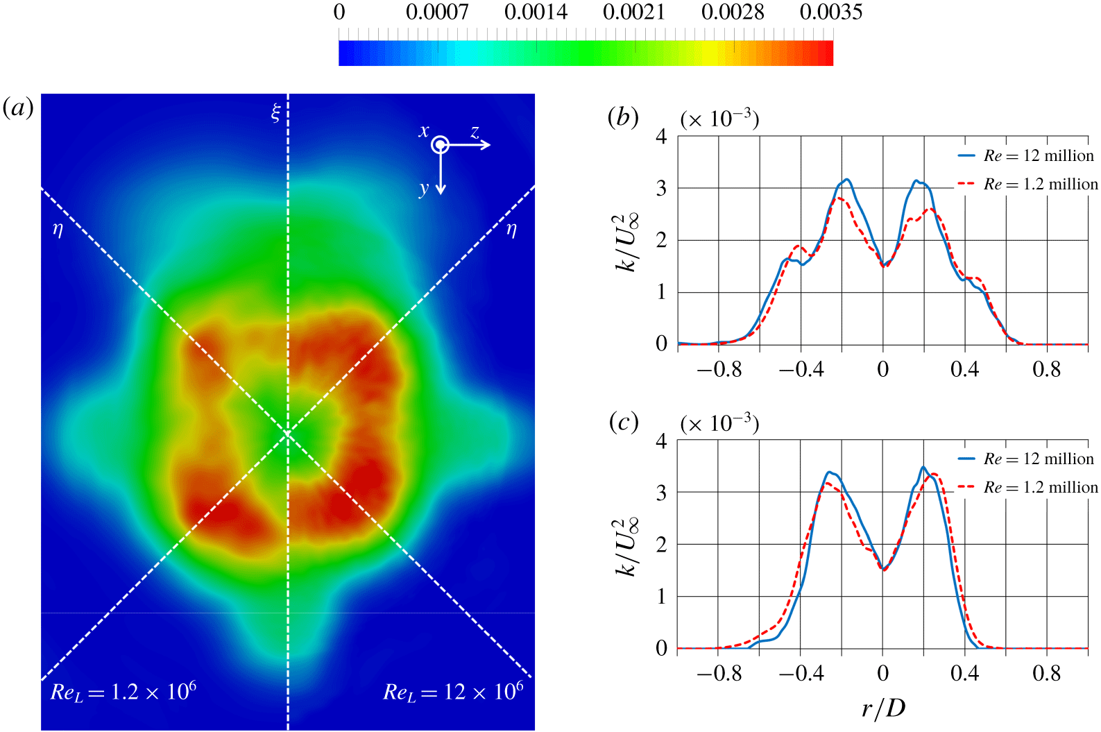
 $\unicode[STIX]{x1D709}$ show two maxima on each side. The outer ones are due to the tip flows from the stern appendages, while the inner ones to the junction flows. This azimuthal coordinate is strongly affected by the wake of the appendages, especially the fins. Therefore, turbulence is higher at the lower Reynolds number. Asymmetry is due to the wake of the sail, causing higher turbulence on the left side of figure 29(b). Profiles along
 $\unicode[STIX]{x1D702}$ in figure 29(c) are substantially different. At outer radii values are lower than in figure 29(b), since the influence of the wake of the appendages is missing. Also in this case two maxima are visible on both sides, but the source of the outer ones is different than in figure 29(b). They originate from the thick stern boundary layer, which developed an outer peak of turbulent kinetic energy. As discussed in § 4.2.1, that peak is larger at the lower Reynolds number. In contrast, the inner maxima, associated with the junction vortices, are substantially higher at
 $Re_{L}=12\times 10^{6}$. Therefore, compared to upstream locations, results at the tail of the DSub indicate that junction vortices from the stern appendages develop gradually a more significant role in both first- and second-order statistics at the higher Reynolds number, with a stronger impact on the near wake of the DSub, albeit over most of the stern boundary layer their footprint is rather similar between
 $Re_{L}=1.2\times 10^{6}$ and
 $Re_{L}=12\times 10^{6}$. The discussion in § 4.2.2 pointed indeed to the higher values of circulation within the junction vortices in the latter case, consistent with their growing influence as the wake of the DSub develops downstream.
Contours of turbulent kinetic energy on the horizontal meridian plane ( $y=0$) for
 $Re_{L}=1.2\times 10^{6}$ (a) and
 $Re_{L}=12\times 10^{6}$ (b). Values scaled by
 $U_{\infty }^{2}$.

Turbulent kinetic energy in the wake of the appended DSub for  $Re_{L}=1.2\times 10^{6}$ (a) and
 $Re_{L}=12\times 10^{6}$ (b) on 6 cross-sections between
 $x/D=0$ and
 $x/D=5$. Values scaled by
 $U_{\infty }^{2}$.

The discussion above pointed to the fact that, at the tail, the outer maxima of turbulent fluctuations, associated with the stern boundary layer, are larger at the lower Reynolds number. However, the evolution downstream for  $Re_{L}=1.2\times 10^{6}$ and
 $Re_{L}=12\times 10^{6}$ is different, making the dual peak in the wake slightly stronger at the higher Reynolds number, in agreement with the results reported for the unappended DSub by Jiménez et al. (Reference Jiménez, Hultmark and Smits2010a). Figure 30 shows a comparison of the fields of turbulent kinetic energy in the horizontal plane (
 $y=0$). The boundary layer over the hull is populated by higher values of turbulent kinetic energy for
 $Re_{L}=1.2\times 10^{6}$. Nonetheless, the bimodal distribution in the wake is similar between the two cases, also in quantitative terms, with even slightly higher values for
 $Re_{L}=12\times 10^{6}$. It is also worth noting that, in both cases, the maxima of turbulent kinetic energy experience a slight increase moving downstream, due to azimuthal readjustment of the wake, as we will discuss more in detail later. Turbulence at the trailing edge of the fins is substantially higher than that shed from the stern boundary layer, especially at outer radii, but it fades out very quickly downstream and boundary layer turbulence already dominates the wake signature at only few diameters away from the tail of the DSub.
(a) Contours of turbulent kinetic energy 1 diameter downstream of the DSub for  $Re_{L}=1.2\times 10^{6}$ (left) and
 $Re_{L}=12\times 10^{6}$ (right); (b) profiles along the direction
 $\unicode[STIX]{x1D709}$ shown in (a); (c) profiles along the direction
 $\unicode[STIX]{x1D702}$ shown in (a). Values scaled by
 $U_{\infty }^{2}$.

(a) Contours of turbulent kinetic energy 5 diameters downstream of the DSub for  $Re_{L}=1.2\times 10^{6}$ (left) and
 $Re_{L}=12\times 10^{6}$ (right); (b) profiles along the direction
 $\unicode[STIX]{x1D709}$ shown in (a); (c) profiles along the direction
 $\unicode[STIX]{x1D702}$ shown in (a). Values scaled by
 $U_{\infty }^{2}$.

The azimuthal readjustment of turbulent kinetic energy is well represented in figure 31, where 6 cross-sections are shown between the streamwise locations at  $x/D=0$ and
 $x/D=5$. At the tail distributions are obviously not axisymmetric, with the footprint of the stern appendages easily distinguishable, besides that of the wake of the sail. Values are higher at the lower Reynolds number. In the near-wake turbulence originating from the fins decreases very quickly moving downstream and a stronger bimodal distribution is visible in the planes away from the appendages, with instead lower values at azimuthal coordinates directly aligned with them. However, moving away from the DSub, the turbulence distribution becomes more symmetric, increasing in the planes through the fins, as pointed in the discussion dealing with figure 30. Note also that, at downstream locations, values of turbulent kinetic energy are actually higher at
 $Re_{L}=12\times 10^{6}$. A more quantitative evidence of this trend is provided in figure 32. We have shown above that at the tail maxima of turbulent stresses, associated with the stern boundary layer, are higher at the lower Reynolds number. This is not the case anymore already at
 $1D$ downstream. Figure 32(a) displays a side-by-side comparison between Reynolds numbers. Maxima away from the axis are already very similar. It is also confirmed that in the DSub wake turbulence due to the junction vortices is higher at the higher Reynolds number, as visible at inner radii at azimuthal coordinates closer to the planes of the appendages (
 $y=0$ and
 $z=0$). Profiles in figure 32(b), extracted along the direction
 $\unicode[STIX]{x1D709}$, show for both Reynolds numbers a substantial decrease of the outer maxima, associated with tip flows from the stern appendages, compared to figure 29(b). In contrast, the inner maxima, mainly tied to the junction flows from the root of the fins, are almost unchanged. Furthermore, at this streamwise location they are already slightly higher at the higher Reynolds number, confirming that their footprint in the near wake becomes more significant for
 $Re_{L}=12\times 10^{6}$. Also the profiles along
 $\unicode[STIX]{x1D702}$ in figure 32(c) show interesting results. The outer peaks, associated with turbulence coming from the stern boundary layer, become very similar at this streamwise location, in contrast with the results reported in figure 29(c). The inner maxima, tied to the junction vortices, are again higher for the case at
 $Re_{L}=12\times 10^{6}$, while they are already practically missing at
 $Re_{L}=1.2\times 10^{6}$.
As seen in figure 31, at downstream locations in the wake, the turbulence distribution becomes more axisymmetric, with slightly higher values of turbulent kinetic energy at the higher Reynolds number, especially at azimuthal coordinates aligned with the stern appendages, which is likely a memory of the stronger footprint of the junction vortices. More details are reported in figure 33, via the comparison between the two Reynolds numbers at 5 diameters from the tail, where figure 33(a) deals with the most downstream section in both panels of figure 31. In figure 33(b) the maxima along the direction  $\unicode[STIX]{x1D709}$ are indeed higher at
 $Re_{L}=12\times 10^{6}$, with still some memory of the wake of the fins at outer radii for both Reynolds numbers. Along the direction
 $\unicode[STIX]{x1D702}$ (figure 33c) profiles are very similar between
 $Re_{L}=1.2\times 10^{6}$ and
 $Re_{L}=12\times 10^{6}$. This result is in agreement with the conclusions by Jiménez et al. (Reference Jiménez, Hultmark and Smits2010a), dealing with the development of the wake of the unappended DSub, who reported that the bimodal distribution of turbulence in the near wake is weakly dependent on Reynolds number, with only slightly lower fluctuations at the lowest value they investigated, equal to
 $Re_{L}=1.1\times 10^{6}$. We also verified that less coherent structures populate the wake of the DSub at the lower Reynolds number. This is shown in figure 34, where the
 $Q$-criterion was utilized. The bimodal distribution seen for the turbulent kinetic energy fields is very well distinguishable also in terms of wake coherence, but at
 $Re_{L}=1.2\times 10^{6}$ the structures originating from the stern boundary layer in figure 34 extend up to smaller distances downstream. At both Reynolds numbers the signature of the wake shed from the stern appendages is already missing few diameters downstream of the tail of the DSub, which is also consistent with the results reported for the statistics in the wake.
Instantaneous visualization of coherent structures using the  $Q$-criterion at
 $Re_{L}=1.2\times 10^{6}$ (a) and
 $Re_{L}=12\times 10^{6}$ (b) (
 $QD^{2}/U_{\infty }^{2}=80$). Coloured by streamwise velocity, scaled by
 $U_{\infty }$.

5 Conclusions
Results were reported of LES computations on the fully appended DSub at  $Re_{L}=12\times 10^{6}$ in towed conditions, providing also a comparison with the case at
 $Re_{L}=1.2\times 10^{6}$ from our earlier study in Posa & Balaras (Reference Posa and Balaras2016a). Computations were performed adopting a wall-modelling strategy over the cylindrical mid-body, where the boundary layer is in equilibrium, with pressure gradient and curvature effects being negligible. In the wall-modelled region the Spalding profile (Spalding Reference Spalding1961) was utilized to define the boundary conditions at the interface nodes of a cylindrical grid composed of a total of approximately 8.1 billion nodes, in the framework of an immersed-boundary methodology. The simulation at
 $Re_{L}=12\times 10^{6}$ was validated against measurements in the boundary layer for both an appended and unappended DSub by Huang et al. (Reference Huang, Liu, Groves, Forlini, Blanton and Gowing1992) and in the wake of the bare hull by Jiménez et al. (Reference Jiménez, Hultmark and Smits2010a) for the same value of the Reynolds number.
Results show that, over the stern, the boundary layer thickness is severely affected by the adverse pressure gradient, experiencing a significant growth, almost independent of the Reynolds number. The development of an outer peak of turbulent kinetic energy, due to the dramatic decrease of the inner layer turbulence, is faster at  $Re_{L}=1.2\times 10^{6}$, since outer layer turbulence is higher in that case and almost unaffected by pressure gradient. The size of the junction vortices at the stern as well as their effect on the boundary layer flow, both in qualitative and quantitative terms, are similar at the two Reynolds numbers, although values of circulation were found higher at
 $Re_{L}=12\times 10^{6}$. In both cases the interaction with the boundary layer over the stern and the appendages produces secondary vortices and growing values of circulation up to the trailing edge of the fins. Junction vortices bring higher momentum fluid at the root of the appendages and downstream of them, where also higher values of turbulent kinetic energy were observed. Such phenomena occur slightly closer to the surface of the stern at
 $Re_{L}=12\times 10^{6}$ and have a significant impact on the evolution of the stern boundary layer downstream of the fins, decreasing its thickness and contributing additional turbulence. Overall, the influence of the junction vortices on the first- and second-order statistics of most of the stern boundary layer is weakly dependent on the Reynolds number. However, starting from the tail of the DSub the footprint of the junction vortices in the near wake becomes gradually more distinguishable at
 $Re_{L}=12\times 10^{6}$ than at
 $Re_{L}=1.2\times 10^{6}$. At the tail of the DSub and immediately downstream, levels of turbulent kinetic energy are indeed higher at
 $Re_{L}=1.2\times 10^{6}$, except at the inner radial coordinates directly affected by the junction vortices coming from the root of the fins. The dual peak of turbulent fluctuations, originating from the stern boundary layer and reinforced by turbulence associated with the junction vortices, is initially stronger at
 $Re_{L}=1.2\times 10^{6}$, but only few diameters away from the DSub it becomes similar between the two Reynolds numbers, with even slightly higher values at
 $Re_{L}=12\times 10^{6}$. This result is in agreement with the findings by Jiménez et al. (Reference Jiménez, Hultmark and Smits2010a), who reported a weak dependence of the maxima of velocity fluctuations in the wake on the Reynolds number. For both
 $Re_{L}=1.2\times 10^{6}$ and
 $Re_{L}=12\times 10^{6}$ an azimuthal readjustment of the wake flow causes increasing values of turbulent kinetic energy over the planes aligned with the stern appendages, due to turbulence coming from the azimuthal locations receiving the outer layer turbulence shed from the stern and that contributed by the junction vortices. Such turbulence sources dominate the wake of the towed DSub at both simulated Reynolds numbers, producing the bimodal distribution of turbulent fluctuations discussed by Jiménez et al. (Reference Jiménez, Hultmark and Smits2010a), observed here also via visualizations of the coherent structures in the wake. In contrast, turbulence and coherence tied to the shear layer shed from the trailing edge of the stern appendages decline very quickly immediately downstream of the DSub. The robustness or these flow phenomena at non-zero yaw and pitch angles is certainly worth investigating via direct numerical simulation, as the flow structures originating from the DSub body can be directly correlated to the wake features. These topics will be addressed in our future work.
Acknowledgements
This work is supported by ONR grant N000141110455, monitored by Dr K.-H. Kim. A.P. is partially supported by the European Union Horizon 2020 research and innovation programme HOLISHIP ‘Holistic Optimisation of Ship Design and Operation for Life Cycle’ under grant agreement n. 689074. Computational time for this work is provided through an allocation from the DoD High Performance Computing Modernization Program (HPCMP). A.P. is grateful to Professor Lippolis for his help and his support for the past several years, first as a teacher and then as a collaborator.
Declaration of interests
The authors report no conflict of interest.