


Impact Statement
This article shows how learned super-resolution can enhance the spatial detail of coarse-resolution weather forecasts without retraining forecasting models at operational resolution. The approach reduces computational requirements, making high-resolution weather products more accessible in research and operational settings with limited resources.
1. Introduction
In recent years, machine learning (ML)-based weather forecasting has advanced significantly, with models now matching or surpassing traditional numerical weather prediction (NWP) systems in forecast skill and inference efficiency (Bi et al., Reference Bi, Xie, Zhang, Chen, Gu and Tian2023; Lam et al., Reference Lam, Sanchez-Gonzalez, Willson, Wirnsberger, Fortunato, Alet, Ravuri, Ewalds, Eaton-Rosen, Hu, Merose, Hoyer, Holland, Vinyals, Stott, Pritzel, Mohamed and Battaglia2023; Lang et al., Reference Lang, Alexe, Clare, Roberts, Adewoyin, Ben Bouallègue, Chantry, Dramsch, Dueben, Hahner, Maciel, Prieto-Nemesio, O’Brien, Pinault, Polster, Raoult, Tietsche and Leutbecher2026). This progress is attributable to the development of increasingly powerful architectures and the availability of high-quality, multi-decadal reanalysis datasets, such as ERA5 (Hersbach et al., Reference Hersbach, Bell, Berrisford, Hirahara, Horányi, Muñoz-Sabater, Nicolas, Peubey, Radu, Schepers, Simmons, Soci, Abdalla, Abellan, Balsamo, Bechtold, Biavati, Bidlot, Bonavita, de Chiara, Dahlgren, Dee, Diamantakis, Dragani, Flemming, Forbes, Fuentes, Geer, Haimberger, Healy, Hogan, Hólm, Janisková, Keeley, Laloyaux, Lopez, Lupu, Radnoti, de Rosnay, Rozum, Vamborg, Villaume and Thépaut2020). This new generation of models enables rapid generation of large ensembles, but training remains computationally demanding: multi-terabyte, high-resolution datasets impose severe data throughput and memory constraints, which typically require access to large-scale computational resources (Bonev et al., Reference Bonev, Kurth, Mahesh, Bisson, Kossaifi, Kashinath, Anandkumar, Collins, Pritchard and Keller2025).
At the same time, models trained at coarser spatial resolutions, where data volume and memory requirements are far more manageable, demonstrate that competitive forecast skill can still be achieved (Nguyen et al., Reference Nguyen, Shah, Bansal, Arcomano, Maulik, Kotamarthi, Foster, Madireddy and Grover2024; Verma et al., Reference Verma, Heinonen and Garg2024; Couairon et al., Reference Couairon, Singh, Charantonis, Lessig and Monteleoni2026). This reflects the scale dependence of atmospheric predictability: for medium-range forecasts, skill is primarily constrained by large-scale atmospheric dynamics (Anthes et al., Reference Anthes, Kuo, Baumhefner, Errico and Bettge1985; Moore, Reference Moore2023). However, this reduced-cost regime remains insufficient to resolve the spatial scales that govern regional weather. These are necessary to represent the organization and intensity of the phenomena that drive local impacts, including heavy precipitation, strong winds, and tropical cyclones.
This motivates exploring alternative strategies that decouple spatial resolution from model training cost. Inspired by advances in computer vision, a natural direction is to employ learned super-resolution (SR) methods (Dong et al., Reference Dong, Loy, He and Tang2016; Ledig et al., Reference Ledig, Theis, Huszar, Caballero, Cunningham, Acosta, Aitken, Tejani, Totz, Wang and Shi2017; Saharia et al., Reference Saharia, Ho, Chan, Salimans, Fleet and Norouzi2023), also commonly referred to as downscaling in the climate sciences. Rather than retraining or fine-tuning a forecasting model at higher resolution, SR aims to learn a mapping from coarse to fine spatial scales. This approach offers complementary advantages in modularity and efficiency: the forecasting and the downscaling models can be developed and optimized independently. In this framework, forecasting operates at low resolution, while super-resolution recovers subgrid-scale variability. So far, data-driven downscaling has primarily focused on regional climate applications (Watt and Mansfield, Reference Watt and Mansfield2024; Hess et al., Reference Hess, Aich, Pan and Boers2025; Mardani et al., Reference Mardani, Brenowitz, Cohen, Pathak, Chen, Liu, Vahdat, Nabian, Ge, Subramaniam, Kashinath, Kautz and Pritchard2025), typically operating on individual states and a limited set of target variables, without explicit consideration of forecast trajectories. Notable exceptions include SwinRDM (Chen et al., Reference Chen, Du, Hu, Wang and Wang2023), which combines a coarse-resolution recurrent forecast model with a diffusion-based upsampling step, demonstrating the viability of cascading forecasting and generative downscaling for high-resolution weather prediction. More recently, Climate in a Bottle (Brenowitz et al., Reference Brenowitz, Ge, Subramaniam, Gupta, Hall, Mardani, Vahdat, Kashinath and Pritchard2025) integrates generative downscaling within a climate modeling pipeline to produce kilometer-scale forecasts.
In this work, we apply learned generative super-resolution to global medium-range forecast trajectories produced by coarse-resolution data-driven models. Using ArchesWeatherGen (Couairon et al., Reference Couairon, Singh, Charantonis, Lessig and Monteleoni2026) as a representative forecasting system, we assess whether super-resolution can reconstruct physically meaningful fine-scale structure while remaining consistent with the underlying large-scale dynamics, thereby supporting its feasibility as a modular and computationally affordable pathway toward higher-resolution forecasting. The remainder of the paper is structured as follows. We first introduce the problem formulation and the proposed super-resolution framework. We then describe the generative model and its application to forecast trajectories, followed by the experimental setup, evaluation methodology, and results. Finally, we discuss the implications, limitations, and possible directions for future work.
2. Methods
2.1. Problem formulation
We consider the problem of reconstructing a high-resolution atmospheric trajectory consistent with a given coarse-resolution forecast. Let
$ {\mathbf{x}}_t $
 denote the global weather state at time
$ t $
 . In our framework,
$ {\mathbf{x}}_t $
 consists of six upper-air variables (temperature, geopotential, specific humidity, wind components
$ U $
 ,
$ V $
 , and
$ W $
 ) sampled on a latitude-longitude grid at 13 pressure levels and four surface variables (2 m temperature, mean sea-level pressure, and 10 m wind components
$ U $
 and
$ V $
 ).
2.1.1. Coarse-resolution forecasts
Let
$ {\mathbf{x}}_t^{\mathrm{LR}} $
 denote a low-resolution (LR) atmospheric state at time
$ t $
 . A forecasting model
$ {f}_{\theta } $
 is trained to predict the future state at a fixed lead time
$ \delta $
 ,

where
$ \delta $
 is set to
$ \delta =24\hskip0.22em \mathrm{h} $
 throughout this work. Forecast trajectories of length
$ T $
 are obtained by applying the model autoregressively,

Our objective is to construct corresponding high-resolution (HR) forecasts
$ {\left({\hat{\mathbf{x}}}_{t+ k\delta}^{\mathrm{HR}}\right)}_{1\le k\le T} $
 .
2.1.2. The coarse-graining operator
The relationship between resolutions is formalized through a known regridding operator
$ \mathcal{C} $
 . For any high-resolution state
$ {\mathbf{x}}_t^{\mathrm{HR}} $
 , the associated coarse representation is given by
$ {\mathbf{x}}_t^{\mathrm{LR}}=\mathcal{C}\left({\mathbf{x}}_t^{\mathrm{HR}}\right). $
 By construction,
$ \mathcal{C} $
 removes information associated with unresolved spatial scales and therefore defines a lossy, non-invertible mapping. The super-resolution problem can thus be viewed as learning an approximate inverse operator
$ {\mathcal{C}}_{\phi}^{-1} $
 such that
$ {\hat{\mathbf{x}}}_t^{\mathrm{HR}}={\mathcal{C}}_{\phi}^{-1}\left({\mathbf{x}}_t^{\mathrm{LR}}\right) $
 . A design objective is that reapplying the coarse-graining operator to the reconstructed high-resolution fields approximately recovers the original coarse state,
$ \mathcal{C}\left({\hat{\mathbf{x}}}_t^{\mathrm{HR}}\right)\approx {\mathbf{x}}_t^{\mathrm{LR}}. $
 This reflects the intent to preserve the large-scale organization of the coarse state while enriching it with unresolved structure.
2.1.3. Residual formulation
To structure this inverse problem, we adopt a residual decomposition formally analogous to a Reynolds decomposition, in which a field is expressed as the sum of a resolved component and a fluctuating part (Reynolds, Reference Reynolds1895). Let
$ \mathcal{I} $
 denote a deterministic interpolation operator (e.g., bicubic) mapping coarse-resolution fields to the high-resolution grid, and define
$ \uparrow {\mathbf{x}}_t^{\mathrm{LR}}=\mathcal{I}\left({\mathbf{x}}_t^{\mathrm{LR}}\right). $
 By construction, this interpolated field preserves the large-scale structure of the coarse state but contains no genuine small-scale variability, that is,
$ \mathcal{C}\left(\mathcal{I}\left({\mathbf{x}}_t^{\mathrm{LR}}\right)\right)\approx {\mathbf{x}}_t^{\mathrm{LR}} $
 . The high-resolution state can then be written as
$ {\mathbf{x}}_t^{\mathrm{HR}}=\uparrow {\mathbf{x}}_t^{\mathrm{LR}}+{\mathbf{r}}_t, $
 where
$ \mathbf{r} $
 represents the unresolved high-frequency residual. We train a neural network
$ {g}_{\phi } $
 to predict this residual,
$ {\hat{\mathbf{r}}}_t={g}_{\phi}\left(\uparrow {\mathbf{x}}_t^{\mathrm{LR}}\right), $
 yielding the final reconstruction

This formulation concentrates model capacity on reconstructing fine-scale structure while explicitly preserving the large-scale information already present in the coarse field. Similar residual strategies have proven effective in climate downscaling (Li et al., Reference Li, Carver, Lopez-Gomez, Sha and Anderson2024; Lopez-Gomez et al., Reference Lopez-Gomez, Wan, Zepeda-Núñnez, Schneider, Anderson and Sha2025; Mardani et al., Reference Mardani, Brenowitz, Cohen, Pathak, Chen, Liu, Vahdat, Nabian, Ge, Subramaniam, Kashinath, Kautz and Pritchard2025).
2.1.4. Stochastic inverse modeling
From a physical standpoint, the inverse problem is inherently non-unique: a coarse forecast constrains the large-scale atmospheric flow but does not uniquely determine fine-scale structure. Subgrid variability admits many realizations compatible with the same resolved state. Accordingly, our objective is not to recover a single deterministic field but to learn a stochastic inverse mapping by modeling the conditional distribution of unresolved residuals,
$ p\left({\mathbf{r}}_t|\uparrow {\mathbf{x}}_t^{\mathrm{LR}}\right) $
 . Although we operate on forecast trajectories, we do not explicitly condition the inverse model on temporal history. At 24-hour lead times and 1.5° resolution, fine-scale organization is primarily constrained by the large-scale flow at that time, making additional temporal conditioning weakly informative while increasing model complexity. We empirically verify this in Supplementary Section C.2.
2.2. Super-resolution model
We adopt a conditional generative super-resolution approach inspired by SR3 (Saharia et al., Reference Saharia, Ho, Chan, Salimans, Fleet and Norouzi2023), adapted to the residual formulation and to global weather fields. Instead of the original SR3 U-Net backbone, we use a 3D Swin U-Net transformer architecture as in ArchesWeather (Couairon et al., Reference Couairon, Singh, Charantonis, Lessig and Monteleoni2026), which better scales to high-resolution fields (Crowson et al., Reference Crowson, Baumann, Birch, Abraham, Kaplan and Shippole2024). To model the stochasticity of unresolved scales, we train the model using flow matching (Lipman et al., Reference Lipman, Chen, Ben-Hamu, Nickel and Le2023), learning the conditional distribution
$ p\left({\mathbf{r}}_t|\uparrow {\mathbf{x}}_t^{\mathrm{LR}}\right) $
 . Further architectural details are provided in Supplementary Section A.2.
2.2.1. Application to forecasts
We apply the super-resolution operator as a post-processing step to coarse-resolution forecast states for all lead times (Figure 1a). Given a coarse-resolution forecast trajectory
$ {\left({\hat{\mathbf{x}}}_{t+ k\delta}^{\mathrm{LR}}\right)}_{1\le k\le T} $
 , the corresponding high-resolution fields are obtained independently at each lead time as

Overview of the super-resolution procedure. (a) Super-resolution is applied independently to each coarse-resolution forecast state produced by the base forecasting model. (b) Sampling procedure: starting from Gaussian noise, a flow-matching model generates a high-resolution residual conditioned on the interpolated coarse-resolution forecast, which is added to obtain the final high-resolution prediction.

Figure 1. Long description
Panel a, titled Application to forecasts, shows a horizontal sequence of three forecasting steps. At the top, a blue box labeled Forecasting model receives a low-resolution input x sub t super L R and produces a forecast x hat sub t plus delta super L R. This output feeds into the next Forecasting model in the sequence. Below each low-resolution forecast, a purple box labeled Super-resolution processes the data to produce a high-resolution prediction x hat sub t plus delta super H R, visualized as a detailed global heat map.
Panel b, titled Sampling, shows the denoising process. A vertical column of four global maps begins at the top with Gaussian noise labeled N(0, I). Arrows point downward through a Denoising process. To the left of this column, an interpolated coarse-resolution forecast x hat sub t plus delta super L R with an upward arrow acts as a Conditional input, with arrows pointing to each stage of the denoising column. The final map at the bottom of the column is labeled r sub t plus delta Generated residual. This residual is added via a plus symbol in a circle to the original conditional input to produce the final high-resolution prediction x hat sub t plus delta super H R on the far right.
In the following, we consider ArchesWeatherGen as the coarse-resolution forecasting framework, which is augmented by the proposed super-resolution approach.
3. Experiments
3.1. Training and evaluation data
Training pairs
$ \left({\mathbf{x}}^{\mathrm{LR}},{\mathbf{x}}^{\mathrm{HR}}\right) $
 are constructed by regridding ERA5 data at 0.25° resolution to 1.5° using the first-order conservative scheme. This remapping ensures that fluxes remapped to the coarse grid represent the same net energy and mass exchange as on the fine grid (Jones, Reference Jones1999). This setup corresponds to a
$ 6\times $
 downscaling task in both latitude and longitude. We use data from 1979 to 2018 for training, 2019 for validation, and 2020 for testing.
3.1.1. Zero-shot application to forecasts
Although the super-resolution model is trained exclusively on reanalysis pairs, we apply it to model forecast outputs in a zero-shot manner. This is possible because ArchesWeatherGen is trained to sample physically plausible coarse-resolution trajectories from the ERA5 data distribution. ArchesWeatherGen produces stochastic ensemble members such that multiple forecast realizations correspond to the same reanalysis state. As a result, no unique supervised mapping from forecast outputs to ERA5 exists, whereas training exclusively on ERA5-based pairs yields a well-posed inverse regridding task that is independent of forecast model errors.
3.2. Evaluation methodology
Our experimental evaluation is organized around two complementary objectives: (i) validating the consistency of the super-resolution operator with respect to the underlying coarse-resolution forecasts and (ii) assessing the quality of the resulting high-resolution forecasts in a standard benchmarking setting. In both sets of experiments, each high-resolution ensemble member is obtained by super-resolving the corresponding low-resolution ArchesWeatherGen trajectory.
3.2.1. Design validation
We first assess the impact of super-resolution on coarse-resolution forecasts produced by ArchesWeatherGen at
$ 1.5{}^{\circ} $
 resolution. To this end, we compare re-coarsened super-resolved forecasts against the original ArchesWeatherGen trajectories using pattern correlation, activity ratio, and normalized RMSE. Re-coarsening is performed using the same conservative regridding operator
$ \mathcal{C} $
 used to construct the coarse-resolution training data. Pattern correlation is computed as the Pearson correlation coefficient over the latitude-longitude grid, while the activity ratio and normalized RMSE quantify changes in resolved-scale variance and amplitude, respectively. Precise definitions of each metric are provided in Supplementary Section B.1.
3.2.2. Forecasting benchmark
In a second set of experiments, we evaluate the quality of super-resolved forecasts within a standard global weather forecasting framework. Following the WeatherBench 2 protocol (Rasp et al., Reference Rasp, Hoyer, Merose, Langmore, Battaglia, Russell, Sanchez-Gonzalez, Yang, Carver, Agrawal, Chantry, Ben Bouallegue, Dueben, Bromberg, Sisk, Barrington, Bell and Sha2024) and the experimental setup of ArchesWeatherGen, we compare post-processed high-resolution forecasts against established baselines, including IFS ENS (ECMWF, 2019), GenCast (Price et al., Reference Price, Sanchez-Gonzalez, Alet, Andersson, El-Kadi, Masters, Ewalds, Stott, Mohamed, Battaglia, Lam and Willson2025), and a naive bicubic interpolation of coarse-resolution ArchesWeatherGen forecasts to the target resolution, which serves as the no-added-value baseline. The exact formula for each metric is presented in Supplementary Section B.2.
4. Results
4.1. Design validation
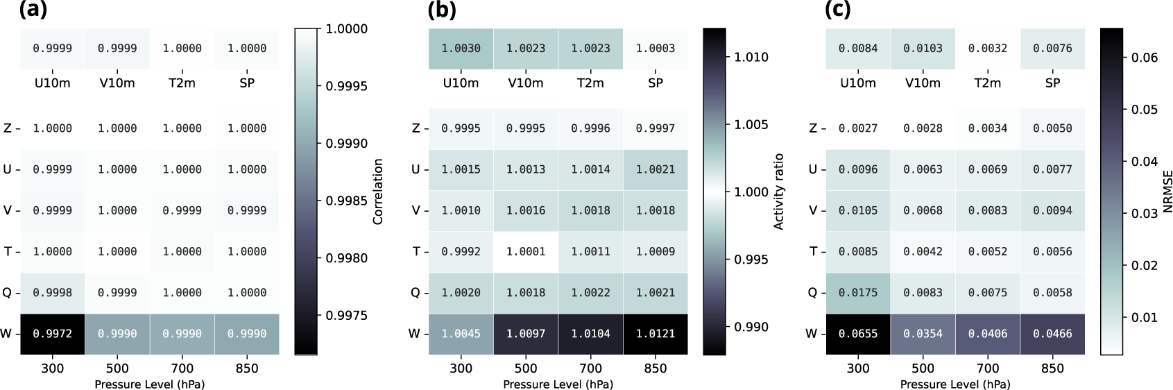
We assess the consistency of the super-resolution design by comparing re-coarsened super-resolved forecasts to the original coarse-resolution trajectories produced by ArchesWeatherGen at a representative lead time of 1 day (Figure 2). This table-based view allows a broader coverage of variables and pressure levels while focusing on a representative short-range lead time. Across all considered surface and upper-air variables, spatial correlations remain extremely close to unity, indicating that the large-scale spatial structure is preserved after super-resolution and re-coarsening. Activity ratios stay near one, ruling out both spurious variance injection and excessive smoothing. Normalized RMSE values remain uniformly small, confirming that reinjecting super-resolved states induces only minor, well-controlled deviations from the original coarse trajectories. Taken together, these diagnostics demonstrate that the proposed super-resolution approach leaves the large-scale state essentially unchanged while introducing only limited and physically consistent subgrid-scale modifications.
Comparison of re-coarsened super-resolved forecasts with the original ArchesWeatherGen coarse-resolution trajectories at 1-day lead time. Shown are (a) spatial correlation, (b) activity ratio, and (c) normalized RMSE, for surface variables and selected pressure levels. Color intensity encodes the deviation from the ideal reference: values approaching white indicate near-perfect agreement (unity for correlation and activity ratio, zero for NRMSE), while darker shades correspond to larger departures from the original coarse-resolution trajectories.

Figure 2. Long description
A three-panel grid of heatmaps. Each panel shares a common X-axis representing Pressure Level in h P a with values 300, 500, 700, and 850. The Y-axis lists atmospheric variables Z, U, V, T, Q, and W. Above the main grid, four surface variables are listed: U 10m, V 10m, T 2m, and S P.
* Panel a Correlation: Values range from 0.9972 to 1.0000. Most cells are white or light gray, indicating near-perfect correlation. The lowest value 0.9972 is at variable W at 300 h P a.
* Panel b Activity ratio: Values range from 0.9992 to 1.0121. The color scale is centered at 1.000 white. Darker shades appear at the bottom row for variable W, particularly at 850 h P a with a value of 1.0121.
* Panel c Normalized R M S E: Values range from 0.0027 to 0.0655. Darker shades indicate higher error. The highest error 0.0655 is located at variable W at 300 h P a. Surface variables show low error ranging from 0.0032 to 0.0103.
Each panel includes a vertical color bar on the right side to map numerical values to color intensity.
4.2. Quality of super-resolved forecasts
We now evaluate the quality of super-resolved forecasts using standard ensemble verification metrics as well as physical consistency diagnostics.
4.2.1. Summary ensemble metrics
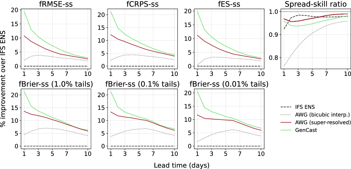
Figure 3 summarizes the performance of the different models using key ensemble metrics, computed in their fair versions: Ensemble Mean RMSE, CRPS, Energy Score (ES), Brier Score, and the spread-skill ratio. Brier Scores are evaluated at symmetric distribution tails by averaging scores at the corresponding lower and upper quantile thresholds (e.g., 1% and 99%). All metrics are expressed as relative improvements with respect to IFS ENS. Scores are averaged over both headline upper-air variables (Z500, Q700, T850, U850, V850) and the four surface variables (T2M, SP, U10M, V10M).
Global ensemble forecast skill at 0.25°. Relative improvement over IFS ENS for fair (
$ f $
 ) ensemble skill-score (
$ ss $
 ) metrics (Ensemble Mean RMSE, CRPS, Energy Score, Brier Score, spread-skill ratio), averaged over WeatherBench headline variables.

Figure 3. Long description
A multi-panel figure with two rows. The y-axis for most panels is percentage improvement over I F S E N S, ranging from 0 to 20. The x-axis for all panels is Lead time in days, ranging from 1 to 10. A legend at the bottom right identifies four models: I F S E N S (dashed black line at 0), A W G bicubic interp. (dotted grey line), A W G super-resolved (solid maroon line), and GenCast (solid light green line).
* Top Row:
1. f R M S E-ss: GenCast starts at 20 percent improvement, decaying to 3 percent by day 10. A W G super-resolved starts at 11 percent, decaying to 2.5 percent. A W G bicubic peaks at day 4 around 4 percent.
2. f C R P S-ss: Similar trends to R M S E, with GenCast starting above 20 percent and A W G super-resolved starting at 12 percent.
3. f E S-ss: Trends mirror the previous panels.
4. Spread-skill ratio: The y-axis ranges from 0.8 to 1.0. I F S E N S is a dashed black line near 0.98. GenCast and A W G super-resolved stay between 0.95 and 1.0. A W G bicubic starts low at 0.76 and rises toward 0.96.
* Bottom Row:
1. f Brier-ss (1.0 percent tails): GenCast starts at 21 percent and decays to 6 percent. A W G super-resolved starts at 14 percent and decays to 6 percent.
2. f Brier-ss (0.1 percent tails): Similar decay, with GenCast and A W G super-resolved converging at 6 percent by day 10.
3. f Brier-ss (0.01 percent tails): GenCast maintains the highest improvement throughout, ending near 7 percent, while A W G super-resolved ends near 6 percent.
Overall, GenCast exhibits the strongest average performance at short to medium lead times (1–7 days). However, ArchesWeatherGen remains competitive and shows comparable skill at longer lead times (7–10 days), particularly for wind components and specific humidity. This behavior is consistent with the increasing dominance of large-scale dynamics at extended lead times. In addition, ArchesWeatherGen displays a more favorable spread-skill ratio across all lead times. While the ensemble remains slightly under-dispersive, this under-dispersion is less pronounced than for GenCast.
4.2.2. Per-variable CRPS analysis
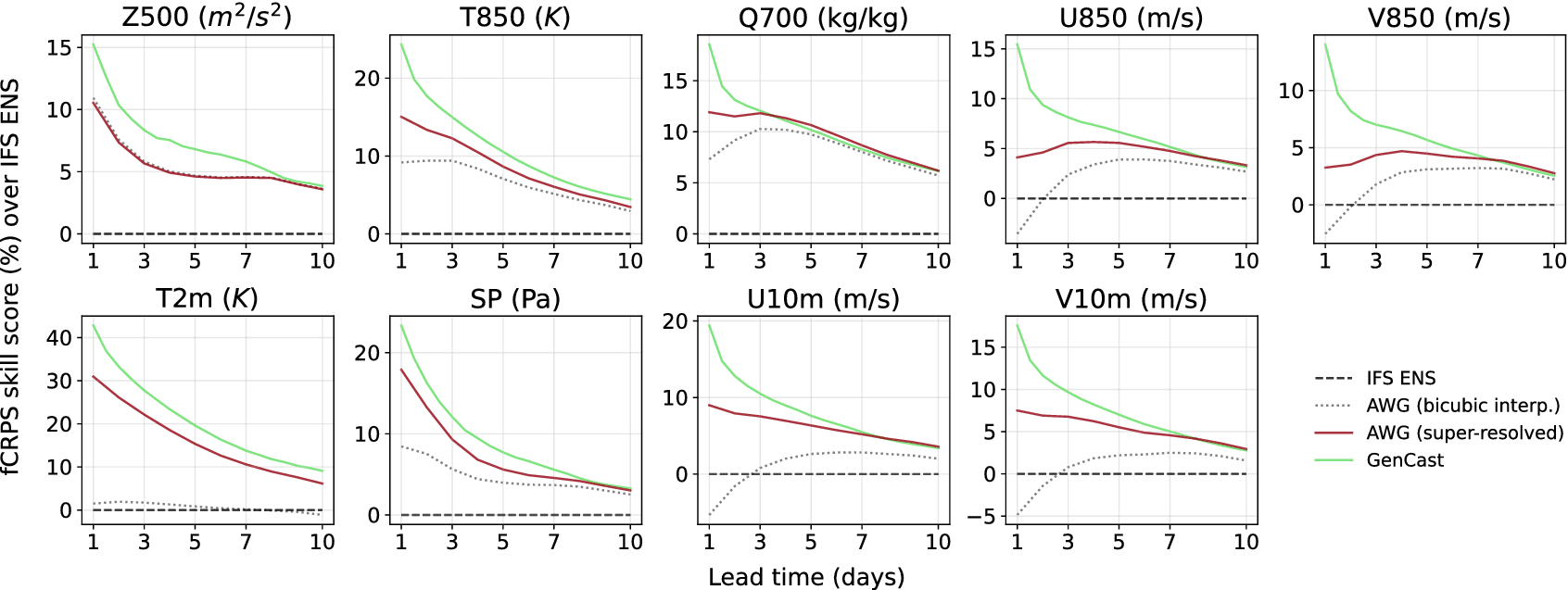
While the previous results focus on metrics averaged across variables, we now examine performance at the level of individual physical variables. Figure 4 reports CRPS skill scores by variable and lead time. We focus on the CRPS, which assesses the quality of the predicted marginal distributions and, when evaluated over long lead times, implicitly penalizes physically inconsistent trajectories in autoregressive models.
Per-variable fair CRPS skill scores relative to IFS ENS at 0.25°. Results are shown for GenCast, and ArchesWeatherGen (AWG) after bicubic interpolation and learned super-resolution, as a function of lead time.

Figure 4. Long description
A multi-panel figure containing nine line graphs arranged in two rows. The y-axis represents f C R P S skill score percentage over I F S E N S, and the x-axis represents Lead time in days from 1 to 10. A legend on the bottom right identifies four lines: a dashed black horizontal line at zero for I F S E N S, a dotted grey line for A W G bicubic interpolation, a solid maroon line for A W G super-resolved, and a solid light green line for GenCast.
Top row panels from left to right:
* Z 500 (m super 2 / s super 2): GenCast starts highest at 15 and decays to 4. A W G super-resolved and bicubic are nearly identical, starting at 11 and decaying to 4.
* T 850 (K): GenCast starts at 25, decaying to 5. A W G super-resolved starts at 15, while bicubic starts at 9; both converge near 4.
* Q 700 (kg / kg): GenCast starts at 18 and decays. A W G super-resolved starts at 12. Bicubic starts at 7, peaks at day 3, then follows the maroon line downward.
* U 850 (m / s): GenCast decays from 15 to 4. A W G super-resolved stays relatively flat between 4 and 6. Bicubic starts negative at -4 and rises to meet the others at day 10.
* V 850 (m / s): Similar to U 850, with GenCast decaying from 14 and bicubic rising from -3.
Bottom row panels from left to right:
* T 2 m (K): GenCast decays from 42 to 10. A W G super-resolved decays from 31 to 6. Bicubic remains flat near zero.
* S P (Pa): GenCast decays from 24 to 4. A W G super-resolved decays from 18 to 4. Bicubic starts at 9 and decays to 3.
* U 10 m (m / s): GenCast decays from 19 to 4. A W G super-resolved decays from 9 to 4. Bicubic starts at -5 and rises to 2.
* V 10 m (m / s): GenCast decays from 18 to 3. A W G super-resolved decays from 8 to 3. Bicubic starts at -5 and rises to 2.
Across all panels, GenCast consistently shows the highest skill score, particularly at shorter lead times, while all models tend to converge as lead time approaches 10 days.
ArchesWeatherGen achieves better CRPS skill scores than IFS ENS across all headline variables and lead times by
$ 7.41\% $
 on average. Compared to GenCast, ArchesWeatherGen exhibits slightly worse performance for lead times of 1–6 days, particularly for wind variables, but achieves similar or better CRPS scores at lead times of 7–10 days. A notable exception is specific humidity, for which ArchesWeatherGen converges to GenCast-level performance at earlier lead times (3–10 days). Relative to bicubic interpolation, the super-resolution approach yields substantially improved probabilistic skill across nearly all variables, with the exception of geopotential. For this variable, bicubic interpolation performs comparatively well due to its intrinsically smooth and large-scale nature. This contrast highlights that the gains from learned super-resolution are most pronounced for variables with richer small-scale variability. We further provide a comparison of fair CRPS skill scores at 1.5° and 0.25° resolutions in Supplementary Section C.3.
4.2.3. Physical consistency and spectral properties
Beyond pointwise probabilistic scores, we assess the physical realism of the generated forecasts through power spectral analysis (Figure 5). Power spectra are computed for selected variables at 1-day and 10-day lead times, with energy averaged across ensemble members. The dashed vertical line marks the transition between scales resolved by the low-resolution forecast (1.5°) and those introduced by super-resolution (0.25°). Both generative models recover substantially more fine-scale energy than bicubic interpolation, demonstrating improved physical consistency at small spatial scales. ArchesWeatherGen exhibits a slightly slower decay of energy at the finest resolved scales compared to GenCast, indicating a better recovery of small-scale variability, although the differences remain moderate. Overall, the spectral analysis confirms that super-resolved forecasts preserve large-scale structure while consistently recovering fine-scale variability.
Comparison of power spectra across models and lead times. Power spectra of Z500, T850, Q700, U850, and V850 at 1-day (top) and 10-day (bottom) lead times. For each model and wavelength, the energy at that wavelength is averaged across samples. The dashed vertical line marks the transition between low- and high-resolution scales (1.5° to 0.25°).

Figure 5. Long description
The multi-panel line graph is organized into two rows and five columns. The top row represents a 1-day lead time and the bottom row represents a 10-day lead time. The columns from left to right represent variables Z 500 (meters-squared per second-squared), T 850 (Kelvin), Q 700 (kilograms per kilogram), U 850 (meters per second), and V 850 (meters per second).
Each graph plots Power Spectrum on the y-axis against Wavelength in kilometers on the x-axis, both on logarithmic scales. The x-axis ranges from 10 super 5 to 10 super 2 kilometers. A vertical dashed line at approximately 600 kilometers marks the transition between low-resolution (1.5 degrees) and high-resolution (0.25 degrees) scales.
Data trends across all panels show a peak in energy at large wavelengths (10 super 4 kilometers) followed by a steep power-law decay as wavelength decreases.
Models compared include:
* E R A 5 (black dashed line)
* GenCast (light green line)
* A W G bicubic interpolation (grey dotted line)
* I F S E N S (blue line)
* A W G super-resolved (dark red line)
In the low-resolution region (left of the dashed line), all models closely overlap with E R A 5. In the high-resolution region (right of the dashed line), the A W G bicubic interpolation line drops significantly below the others, indicating a loss of energy. The GenCast, I F S E N S, and A W G super-resolved lines remain closer to the E R A 5 baseline, though slight divergence occurs at the 10-day lead time, particularly in the Z 500 and V 850 variables where GenCast shows a slight upward curve at the smallest scales.
4.3. Case study: Hurricane Teddy
To complement the quantitative evaluation, we present a case study of Hurricane Teddy, a major Atlantic storm that reached Category 4 intensity in September 2020. It produced one of the most organized deep convective structures of that season. At its peak, Teddy exhibited a well-defined eye, vigorous spiral rainbands, and a broad moisture envelope that spanned much of the subtropical North Atlantic. Figure 6 showcases ArchesWeatherGen super-resolved humidity fields at a 1-day lead time, initialized on September 20, 2020.
Super-resolution of specific humidity at 700 hPa over the North Atlantic (Hurricane Teddy, 21 September 2020 12:00 UTC, +24 h lead time). ERA5 regridded to 1.5° (a) and at native 0.25° (e) serve as low- and high-resolution ground truth, respectively. AWG ensemble forecasts at 1.5° are shown for the best, median, and worst members by RMSE (b–d). Each column of the high-resolution block (f,i,l), (g,j,m), (h,k,n) shows three independent stochastic SR draws at 0.25° for the corresponding LR member. RMSE and bias (g kg
$ {}^{-1} $
 ) against the appropriate ERA5 reference are reported in the top-left corner of each panel.

Figure 6. Long description
A multi-panel set of geographical maps showing specific humidity at 700 h Pa. The color scale on the right ranges from 0 (brown) to 10 (teal) g kg super minus 1.
Top Row (Low-Resolution 1.5 degree):
* Panel a: E R A 5 ground truth showing a pixelated hurricane structure near 30 degrees North, 60 degrees West.
* Panels b, c, and d: A W G ensemble forecasts for best (R M S E 0.80), median (R M S E 0.83), and worst (R M S E 0.87) members.
Second Row (High-Resolution 0.25 degree):
* Panel e: E R A 5 native high-resolution ground truth showing sharp, swirling moisture filaments around the hurricane eye.
* Panels f, g, and h: First set of stochastic super-resolution draws for the best, median, and worst members respectively. R M S E values range from 1.00 to 1.05.
Third Row:
* Panels i, j, and k: Second set of independent stochastic draws for the same three members. R M S E values range from 0.99 to 1.06.
Bottom Row:
* Panels l, m, and n: Third set of independent stochastic draws. R M S E values range from 1.00 to 1.06.
Across all super-resolution panels (f through n), the model reconstructs fine-scale turbulent structures and sharp gradients that are absent in the 1.5 degree inputs, closely mimicking the visual texture of the native 0.25 degree E R A 5 reference in panel e.
At 1.5° resolution, the low-resolution ensemble members (b–d) accurately capture the large-scale moisture distribution and the hurricane’s position, aligning closely with the ERA5 reference (a). Ensemble spread is visible in the representation of the cyclone core: it is less well-defined in the worst-performing member (d) than in the median (c) and best (b) members, while the synoptic-scale flow and storm placement remain consistent across all members. Super-resolution is then applied to each low-resolution member (f–n). At 0.25°, the SR model reconstructs fine-scale structures, including cyclonic moisture spirals, indications of a dry intrusion on the western flank, and sharper outer gradients. For each member, multiple stochastic draws produce distinct realizations that differ in the positioning of small-scale moisture filaments while preserving the large-scale organization inherited from the conditioning low-resolution state. Importantly, this behavior holds consistently across lead times: Supplementary Section C.5 shows that analogous fine-scale structures are recovered at 7-day lead time, demonstrating that the SR model produces physically plausible reconstructions throughout the forecast horizon. It should be noted that such stochastic variability does not necessarily improve forecast skill. Since the SR model is conditioned on the low-resolution input, large-scale errors are not corrected and propagate to the super-resolved outputs. Probabilistic scores may, therefore, penalize the ensemble if it is misaligned with the reference, despite exhibiting realistic fine-scale variability. Nevertheless, by representing physically plausible subgrid structures, super-resolution enables the exploration of internal variability and provides a more complete depiction of uncertainty at fine scales, which is particularly relevant for intense systems such as tropical cyclones. To further quantitatively evaluate the model’s capacity beyond open-ocean dynamics, we extend the analysis to a topographically complex region during the passage of Storm Alex over the Alps (Supplementary Section C.6).
5. Discussion
We investigated learned super-resolution as a modular extension to global weather forecasting models trained at coarse spatial resolution. By decoupling forecasting and downscaling, our approach enables the reconstruction of physically plausible fine-scale structure while preserving the large-scale dynamics learned at low resolution, without retraining forecasting models at operational resolution. Despite its modest computational cost, this strategy achieves competitive forecast performance relative to substantially more expensive end-to-end high-resolution forecasting models.
5.1. Generality and scope
Although demonstrated using the ArchesWeatherGen framework, the proposed approach is not tied to a specific forecasting architecture. In principle, it can be applied to any forecasting model provided that (i) its coarse-resolution outputs represent physically realistic large-scale flow and (ii) its temporal sampling is consistent with the dynamics it resolves. In this work, we focused on daily (24 h) forecast trajectories, a setting in which the method reliably reconstructs fine-scale spatial structure while preserving the underlying coarse-resolution forecast trajectory at the resolved time scale. Extending such daily trajectories to sub-daily (e.g., hourly) outputs would require a dedicated temporal super-resolution component, which we leave for future work. Moreover, by building on probabilistic forecasts rather than deterministic forecasts, the approach naturally decouples large- and fine-scale uncertainties, allowing each to be modeled and sampled independently. Extending the method to deterministic, smoothed inputs would instead require learning a direct or unpaired mapping from forecast outputs to high-resolution reference data (Wan et al., Reference Wan, Baptista, Boral, Chen, Anderson, Sha and Zepeda-Núñez2023; Keisler et al., Reference Keisler, Charantonis, Goude, Oueslati and Monteleoni2026).
5.2. Broader implications
Beyond medium-range weather forecasting, our framework naturally extends to sub-seasonal and climate applications, where large-scale dynamics are generally well represented but fine-scale variability remains under-resolved. In this context, super-resolution models could be trained on high-resolution climate simulations or reanalysis-derived datasets and applied in a zero-shot manner to coarse global climate models, as demonstrated in related work (Hess et al., Reference Hess, Aich, Pan and Boers2025). A particularly promising avenue is the use of global or limited-area kilometer-scale models, such as ICON (Hohenegger et al., Reference Hohenegger, Korn, Linardakis, Redler, Schnur, Adamidis, Bao, Bastin, Behravesh, Bergemann, Biercamp, Bockelmann, Brokopf, Brüggemann, Casaroli, Chegini, Datseris, Esch, George, Giorgetta, Gutjahr, Haak, Hanke, Ilyina, Jahns, Jungclaus, Kern, Klocke, Kluft, Kölling, Kornblueh, Kosukhin, Kroll, Lee, Mauritsen, Mehlmann, Mieslinger, Naumann, Paccini, Peinado, Praturi, Putrasahan, Rast, Riddick, Roeber, Schmidt, Schulzweida, Schütte, Segura, Shevchenko, Singh, Specht, Stephan, von Storch, Vogel, Wengel, Winkler, Ziemen, Marotzke and Stevens2023), as sources of high-resolution reference data.
5.3. Efficiency and limitations
A key advantage of the proposed approach is computational efficiency. Training the full pipeline—deterministic forecasting, generative forecasting, and super-resolution—is on the order of 30 A100-days in total. Super-resolution training represents a relatively small fraction of this cost, requiring approximately 7 A100-days, compared to about 23 A100-days for training ArchesWeatherGen. At inference time, generating a full 10-day high-resolution forecast takes about 8 minutes on a single NVIDIA V100 32GB GPU, which can become significant when applied at scale, such as for long test sets or large ensembles. This computational cost motivates future work on speeding up inference through distillation or consistency-based generative modeling (Stock et al., Reference Stock, Arcomano and Kotamarthi2025).
5.4. Conclusion
Overall, this work demonstrates that learned super-resolution provides a physically grounded and computationally efficient pathway toward higher-resolution weather and climate prediction. By separating large-scale prediction from fine-scale reconstruction, the proposed framework offers flexibility, interpretability, and scalability across forecasting horizons and application domains. Our results demonstrate that this approach achieves competitive forecast skill at operational resolution with substantially reduced computational cost and that recovered small-scale variability exhibits realistic spectral characteristics.
Supplementary material
The supplementary material for this article can be found at http://doi.org/10.1017/eds.2026.10046.
Data availability statement
The ERA5 reanalysis data used in this study are publicly available from the Copernicus Climate Data Store (https://doi.org/10.24381/cds.adbb2d47). The code used in this study is available at https://doi.org/10.5281/zenodo.19355356.
Acknowledgments
The authors thank Guillaume Couairon, David Landry, and Pierre Garcia for fruitful discussions. The authors used Claude (Anthropic) to assist in drafting portions of this manuscript. All content was reviewed and revised by the authors.
Author contribution
Conceptualization: A.D. and A.C. Data curation: A.D. Formal analysis: A.D. Methodology: A.D. Software: A.D. Supervision: A.C. and D.B. Validation: A.D., A.C., and D.B. Visualization: A.D. Writing—original draft: A.D. Writing—review and editing: A.C. and D.B. All authors approved the final submitted draft.
Provenance statement
This article is part of the Climate Informatics 2026 proceedings and was accepted in Environmental Data Science on the basis of the Climate Informatics peer review process.
Competing interests
The authors declare none.
Ethics statement
The research meets all ethical guidelines, including adherence to the legal requirements of the study country.
Funding statement
This work was supported by the French National Research Agency (ANR) and the Ministry of Higher Education and Research. This project was granted HPC resources by GENCI at IDRIS under the allocation AD011016443 on the Jean-Zay supercomputer.





 Open access

