2 Geometrical shock dynamics for fast MHD shocks

3 Comparison of MHD-GSD with full ideal MHD

We test the model with a nonlinear second-order finite-volume solver for the full ideal MHD equations (CMHD) (Samtaney et al. Reference Samtaney, Colella, Ligocki, Martin and Jardin2005). The test case is cylindrical shock collapse in the presence of a spiral magnetic field defined by

where $b$ is a real positive parameter. This spiral magnetic field is solenoidal on $r>0$ . For appropriate choices of $b$ , it allows an oblique orientation of the field to the collapsing shock normal. Behind the shock, particle paths are not radial and do not coincide with rays normal to the shock surface. This then tests the effect of downstream path–ray divergence on the present formulation of MHD-GSD.

The initial conditions for the cylindrical shock are an initial radius of $r_{0}=100$ at an initial preshock magnetosonic Mach number of $M_{f0}=2$ , and we consider values of $b=0.1,1.0,3.0,10.0$ . For the numerical method used in the GSD code, the scale factors are $\unicode[STIX]{x1D70E}=r_{0}e^{-\unicode[STIX]{x1D709}},\unicode[STIX]{x1D70F}=2\unicode[STIX]{x03C0}r_{0}e^{-\unicode[STIX]{x1D709}}$ .

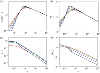
The key variables for comparison are the $M_{f}$ , postshock variables $p$ , tangential magnetic field $B_{\unicode[STIX]{x1D703}}$ , and tangential velocity $u_{\unicode[STIX]{x1D703}}$ , the latter two of which sufficiently account for the oblique postshock particle paths. The comparison is shown in figure 1. The largest discrepancy is observed in postshock pressure $p(r)$ of $9\,\%$ in the peak value. This difference between shock dynamics and the full nonlinear equations is consistent with that seen in previous studies such as Pullin et al. (Reference Pullin, Mostert, Wheatley and Samtaney2014), suggesting that the introduction of the oblique field into MHD shock dynamics has not significantly affected the effectiveness of the approximation. Presently, the presence of downstream path–ray divergence does not appear to compromise the performance of MHD-GSD, suggesting that this is not an important feature of the general GSD framework.

Figure 1.

Comparison between MHD-GSD and CMHD of fast magnetosonic Mach number and three key postshock variables for cylindrical shock collapse in a spiral magnetic field: —, MHD-GSD; - -, CMHD. The CMHD results run with 8000 cells in $r$ , the GSD results at $\unicode[STIX]{x0394}\unicode[STIX]{x1D709}=1\times 10^{-3}$ . On the far left of each panel (a), (b), (d), from top to bottom, $b=0.1,1.0,3.0,10.0$ ; (c), from bottom to top, $b=0.1,1.0,3.0,10.0$ .

4 Stability of plane fast MHD shocks

Consider a simple problem of planar shock propagation in an infinitely wide channel. Planar gas-dynamic shocks are known to be stable in the sense that small initial perturbations decay to zero amplitude over large time (Whitham Reference Whitham2011). The stability of planar MHD shocks is less well studied, but see Trakhinin (Reference Trakhinin2003). Whitham (Reference Whitham2011) argues briefly that an initially smooth disturbance on a planar gas-dynamic shock will undergo wave steepening so that discontinuities on the shock surface, or shock-shocks, form following an initial disturbance.

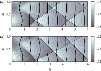
We consider initially planar shocks with sinusoidal perturbation in Mach number $M_{0}=M_{r}\,[1+\unicode[STIX]{x1D716}\,\sin \left(2\unicode[STIX]{x03C0}\,y/\unicode[STIX]{x1D706}\right)]$ , where $y$ is the dimension along the initial planar shock, and $M_{r}=1.8,\unicode[STIX]{x1D706}=1,\unicode[STIX]{x1D716}=0.06$ in this case. Here, $\unicode[STIX]{x1D716}$ is chosen to expose a sizeable perturbation whose motion on the shock may be discerned easily. Figure 2(a) shows the resulting flow pattern for gas-dynamic shocks. The shock travels from left to right and is shown with thick vertical lines, with perturbations on the shock surface exaggerated fivefold. Local $M$ , whose contours can be considered to be characteristics of the disturbance motion along the shock, is shown by shaded colour. Shock-shocks first occur where a kink, or point of infinite curvature, appears on the shock profile, accompanied by the appearance of a discontinuity in $M$ . The onset of shock-shocks can be seen by $M$ contour-gradient steepening followed by the diamond-like formations signalling $M$ discontinuities. These diamonds appear symmetric around their major axes, since disturbances travelling up and down the shock surface have the same strengths and speeds.

Figure 2.

Contours showing successive shock position, moving left to right. Shock position is given by thick vertical lines with perturbation amplitude exaggerated fivefold and local $M$ by faint contours and colour. The colour at a given location shows the shock $M$ when it passed through that location. (a) Gas-dynamic shock; (b) MHD shock, $|B|_{0}=1.55$ , $\unicode[STIX]{x1D719}_{0}=0.199$ . Shocks are initially flat, but perturbed sinusoidally in $M$ with $\unicode[STIX]{x1D716}=0.06$ , $M_{r}=1.8$ .

Figure 2(b), however, shows an equivalent MHD shock for upstream $|B|=1.55,\unicode[STIX]{x1D719}=0.199$ radians, perturbed with the same variation in $M_{0}$ . The general pattern is similar to the gas-dynamic case but there is a clear directional preference in the developed flow. This symmetry-breaking effect is an interesting feature of MHD shocks in oblique magnetic fields, and is caused by the generation of a non-zero downstream tangential velocity that intensifies with increasing magnetic-field strength and decreasing orientation. Indeed, the conditions for figure 2(b) are chosen to make this effect particularly noticeable.

We now seek to quantify the time $t_{B}(\unicode[STIX]{x1D716})$ to first shock-shock formation. A sequence of GSD calculations was performed for both gas-dynamic and MHD shocks over a range of $\unicode[STIX]{x1D716}$ . Shock-shocks are detected as discontinuities in $M$ by an edge-detection algorithm (Gelb & Tadmor Reference Gelb and Tadmor2000, Reference Gelb and Tadmor2006) with a minmod limiter giving a switch between an exponential concentration factor kernel (high order) away from shock-shocks and a first-order polynomial kernel close to shock-shocks, limiting spurious oscillations in the detector. A nonlinear enhancement technique was used to remove small jumps on the grid scale in the discretized solution while allowing $O(M_{r}\unicode[STIX]{x1D716})$ jumps, which correspond to shock-shocks, using a tuning parameter chosen to reflect the expected minimum magnitude of the shock-shock when it forms. The time $t_{B}$ is when the edge detector first gives a non-zero result, and is largely insensitive to plausible choices of the tuning parameter. Parameters used for the nonlinear enhancement technique give resolution-converged results with ${<}1\,\%$ discrepancy between resolutions of $N_{\unicode[STIX]{x1D702}}=2048$ and 4096.

We use uniform upstream magnetic fields of strength $B_{0}=0.5,1,1.5$ and initial upstream orientation $\unicode[STIX]{x1D719}=\unicode[STIX]{x03C0}/4,\unicode[STIX]{x03C0}/2$ , along with a gas-dynamic case. Values of $\unicode[STIX]{x1D716}=4\times 10^{-3},6\times 10^{-3},8\times 10^{-3},1\times 10^{-2},2\times 10^{-2},4\times 10^{-2},8\times 10^{-2}$ are considered with $M_{r}=1.8$ . The scale factors in the numerical method are $\unicode[STIX]{x1D70E}=\unicode[STIX]{x1D70F}=1$ , and the numerical resolution $\unicode[STIX]{x0394}\unicode[STIX]{x1D709},\unicode[STIX]{x0394}\unicode[STIX]{x1D702}$ for these problems is $\unicode[STIX]{x1D716}/20,\unicode[STIX]{x1D706}/2048$ . 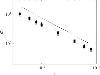Figure 3 shows variation of $t_{B}$ over the $\unicode[STIX]{x1D716}$ considered. A power law $\unicode[STIX]{x1D716}^{-m}$ with exponent close to $m=-1$ is observed across all cases, independent of field strength or orientation. This result can be understood by developing analysis alluded to in passing by Whitham (Reference Whitham2011). The characteristic form of the shock-dynamic equations (2.8) may be written in coordinates $(\unicode[STIX]{x1D6FC},\unicode[STIX]{x1D6FD})$ normal and tangential to the shock as

where $R$ is a Riemann invariant and $\unicode[STIX]{x1D703}$ describes the angle of the local shock normal to some reference axis (for example $x$ ). Here and subsequently, primes indicate differentiation. In (4.1), the $\unicode[STIX]{x1D719},x$ dependence in $A(M,\unicode[STIX]{x1D719},x)$ has been suppressed for clarity.

Figure 3.

Shock-shock formation times $t_{B}$ over initial Mach-number relative disturbance amplitude $\unicode[STIX]{x1D716}$ : $\times$ , gas-dynamic shock; ▾, ▪, ▴, upstream $|B|=0.5,1.0,1.5$ ; filled, unfilled, upstream field orientation $\unicode[STIX]{x1D719}=\unicode[STIX]{x03C0}/2,\unicode[STIX]{x03C0}/4$ ; – –, power law, $t_{B}\sim \unicode[STIX]{x1D716}^{-1}$ expected from the theoretical analysis.

In gas dynamics, $M,c$ have smooth representations $M(R),c(R)$ . We assume that this holds for MHD with $M_{f}>1$ . Now, considering only one family of characteristics and ignoring wave interactions, a nonlinear wave equation can be obtained with wavespeed $c(R)$ ,

where (4.2b ) is a conservation form with $Q^{\prime }(R)=c(R)$ . Now, for an initial condition $R(\unicode[STIX]{x1D6FD}_{0})$ at $\unicode[STIX]{x1D6FC}=0$ , (4.2) has a continuous solution

and at discontinuities (shock-shocks) with speed $S$ the conservation law requires

where subscripts $1,2$ indicate upstream and downstream states respectively and the right-hand side of (4.4) follows from linearizing $c(R)$ , allowing quadratic $Q(R)$ . The solution can thus be written entirely in terms of $c$ , which in this form is also a weak solution to the inviscid Burgers equation (and conservation form), simplifying the problem further,

The first value $\unicode[STIX]{x1D6FC}_{B}$ at which shock-shocks form can be calculated as a function of the initial distribution $c(\unicode[STIX]{x1D6FD}_{0})$ as (Whitham Reference Whitham2011) $\unicode[STIX]{x1D6FC}_{B}=1/|c^{\prime }(\unicode[STIX]{x1D6FD}_{0})|$ , corresponding, by definition of $\unicode[STIX]{x1D6FC}$ , to a shock-shock formation time $t_{B}=(a_{0}|c^{\prime }(\unicode[STIX]{x1D6FD}_{0})|)^{-1}$ .

For an initially sinusoidal, or indeed any continuous periodic distribution of $c$ on the shock with amplitude proportional to $\unicode[STIX]{x1D716}$ , this implies $t_{B}\sim 1/\unicode[STIX]{x1D716}$ to leading order, in agreement with the numerical GSD results. This indicates that $t_{B}$ depends only upon the initial distribution in $c$ and is independent of the $A$ – $M$ relation and therefore of whether the shock is of gas-dynamic or MHD type. Higher-order effects would include the influence of the other characteristic family corresponding to the minus sign in (4.1), which has been ignored here.

5 Stability of converging cylindrical fast MHD shocks

We now consider stability of cylindrical converging MHD shocks. The azimuthal field is given by (3.1) with $b=0$ and the shock is initialized as in § 4 with $M_{r}=5.0,\unicode[STIX]{x1D716}=0.06$ . Scale factors are set as in § 3. The simulation is run on one wavelength, $\unicode[STIX]{x1D706}=2\unicode[STIX]{x03C0}/k$ , with wavenumber $k=20$ and initial radius $r_{0}=1$ . These conditions are chosen to promote short time to shock-shock formation. 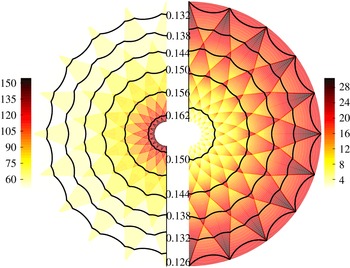The resolution is $N_{\unicode[STIX]{x1D702}}=1024$ , $\unicode[STIX]{x0394}\unicode[STIX]{x1D709}=0.003$ (recall that $\unicode[STIX]{x1D709},\unicode[STIX]{x1D702}$ are curvilinear coordinates). Figure 4 shows the gas-dynamic (left) and MHD (right) shock convergence between the inner and outer radii $r_{in}=0.027,r_{out}=0.3$ and extended periodically to $10$ wavelengths around a half-circle. The colour shows the local postshock pressure and the black line values show $\unicode[STIX]{x1D6FC}$ , which is proportional to $t$ , for the shock position contours.

Figure 4.

Contour maps for cylindrical converging gas-dynamic (left) and MHD (right) shocks. The azimuthal extent of the simulation domain is one wavelength. The inner and outer radii are $r_{in}=0.027,r_{out}=0.3$ . Black contours show successive shock positions, with labels on the top (bottom) half corresponding to gas-dynamic (MHD) shock positions $\unicode[STIX]{x1D6FC}\propto t$ . Shock perturbation amplitudes are exaggerated fourfold. The colour maps indicate local postshock pressure (note the different colour scales). The colour at a given location shows the pressure downstream of the shock as it passes that location. While both shocks exhibit the same polygonal instability, the MHD shock sees a progressive decrease in postshock pressure, in direct contrast to the gas-dynamic shock, and accelerates at a greater rate.

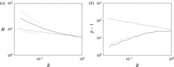
The MHD shock accelerates faster than the gas-dynamic shock. Indeed, figure 5 shows that the gas-dynamic Mach number averaged along the shock approaches an $\bar{R}^{-1}$ asymptote in the MHD case, where $\bar{R}$ is the mean shock radius, compared with $\bar{R}^{-1/n}$ for the gas-dynamic shock, with $n=1+2/\unicode[STIX]{x1D6FE}+(2\,\unicode[STIX]{x1D6FE}/(\unicode[STIX]{x1D6FE}-1))^{1/2}$ and $1/n=0.225425$ for $\unicode[STIX]{x1D6FE}=5/3$ (Whitham Reference Whitham2011). Moreover, unlike the gas-dynamic shock, where the postshock pressure $p$ becomes singular as $\bar{R}\rightarrow 0$ , the converging MHD shock sees $p\sim 1+A\,\bar{R}\ldots$ , $\bar{R}\rightarrow 0$ , where $A$ is a positive constant, as in the unperturbed result (Pullin et al. 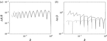Reference Pullin, Mostert, Wheatley and Samtaney2014). Figure 6(a) shows that both shocks have similar profiles in $\unicode[STIX]{x0394}R/\bar{R}$ , where $\unicode[STIX]{x0394}R=R_{max}-R_{min}$ is the peak-to-trough variation of shock radius $R$ along its surface, exhibiting the weak instability noted by Schwendeman (Reference Schwendeman1993) and others. Figure 6(b) shows that the MHD shock instability differs from the gas-dynamic shock in the variation of postshock pressure, $\unicode[STIX]{x0394}p/\bar{p}$ , defined similarly, which grows with decreasing $\bar{R}$ in the MHD case while remaining sensibly constant for the gas-dynamic shock. In addition to the weakening of the shock on collapse in the mean, the MHD shock then also shows a greater relative pressure fluctuation in comparison to the gas-dynamic case. We remark that the hodograph transformation of Whitham (Reference Whitham2011) admits analysis of the perturbed shock collapse for the gas-dynamic case but is not simply extensible to the present MHD case.

Figure 5.

Variation of mean Mach number, pressure over radius: (a) —, $\bar{M}$ for MHD shocks; – –, $\bar{M}$ for gas-dynamic shocks; $\cdots \,$ , $M\sim \bar{R}^{-1/n}$ , gas-dynamic asymptote; – $\cdot$ – $\cdot$ , $M\sim \bar{R}^{-1}$ , MHD asymptote; (b) —, $\bar{p}-1$ for MHD shocks; – –, $\bar{p}-1$ for gas-dynamic shocks; $\cdots \,$ , $\bar{p}-1\sim \bar{R}$ , MHD asymptote.

Figure 6.

Graphs of shock variation in geometry, $\unicode[STIX]{x0394}R/\bar{R}$ (a) and postshock pressure $\unicode[STIX]{x0394}p/\bar{p}$ (b), on the shock as it converges: —, MHD shock; – –, gas-dynamic shock. Here, $\unicode[STIX]{x0394}R$ is the total variation of shock radius along its surface and $\bar{R}$ is its mean radius; $\unicode[STIX]{x0394}p/\bar{p}$ is defined similarly.

6 Concluding remarks

A formulation of GSD has been developed for fast shocks in ideal MHD and implemented numerically using a pseudospectral method. Application to a cylindrically symmetric converging MHD shock in the presence of a non-uniform upstream field at an oblique angle gives satisfactory comparison with results from numerical solutions of the full MHD equations. A novel application to the nonlinear stability of planar fast MHD shocks indicates a time to shock-shock formation inversely proportional to the initial Mach-number perturbation amplitude, in agreement with a simple model based on the Burgers equation. A further comparison between converging MHD and gas-dynamic shocks exposes a notable difference in the postshock pressure variation along the shock, showing a greater growth in pressure fluctuation for the MHD case over the gas-dynamic convergence. The present MHD-GSD approach is expected to be useful in studies of general MHD shock behaviour.