1. Introduction
In the past three decades, computations of invariant solutions of the Navier–Stokes equations have considerably advanced the understanding of subcritical transition to turbulence in wall-bounded shear flows. Invariant solutions, or ‘exact coherent structures’, (Graham & Floryan Reference Graham and Floryan2021) have been computed primarily in pipe flow, plane Couette flow and plane Poiseuille flow (Graham & Floryan Reference Graham and Floryan2021 and references therein). Nagata (Reference Nagata1990) calculated the first known pair of finite-amplitude, nonlinear equilibrium solutions for plane Couette flow using a numerical continuation technique, continuing wavy vortex flow from the Taylor–Couette to plane Couette conditions. The same solution was independently found by Clever & Busse (Reference Clever and Busse1992) and Waleffe (Reference Waleffe2001). Numerous equilibria and travelling waves have since been found for the shear flows mentioned above. For example, see Clever & Busse (Reference Clever and Busse1997), Waleffe (Reference Waleffe1998), Faisst & Eckhardt (Reference Faisst and Eckhardt2003), Wedin & Kerswell (Reference Wedin and Kerswell2004) and Gibson, Halcrow & Cvitanović (Reference Gibson, Halcrow and Cvitanović2009). Periodic and relative periodic orbits have also been computed for plane Couette flow (see Kawahara & Kida Reference Kawahara and Kida2001; Viswanath Reference Viswanath2007; Cvitanović & Gibson Reference Schneider, Gibson and Burke2010), plane Poiseuille flow (Toh & Itano Reference Toh and Itano2003) and pipe flow (Duguet, Willis & Kerswell Reference Duguet, Willis and Kerswell2008). Relatively fewer solutions have been computed for plane Poiseuille flow (see Ehrenstein & Koch Reference Ehrenstein and Koch1991; Waleffe Reference Waleffe1998; Toh & Itano Reference Toh and Itano2003; Waleffe Reference Waleffe2003; Gibson & Brand Reference Gibson and Brand2014; Park & Graham Reference Park and Graham2015; Zammert & Eckhardt Reference Zammert and Eckhardt2015). Much of this work is restricted to small periodic domains.
Another line of work has been to study transitional turbulence in large periodic domains (see Tuckerman, Chantry & Barkley (Reference Tuckerman, Chantry and Barkley2020) and references therein). Large periodic domains allow for complex phenomena such as spatial localisation, because longer wavelengths can be incorporated. In large domains, localised puffs in the case of pipe flow (Avila et al. Reference Avila, Moxey, de Lozar, Avila, Barkley and Hof2011) and bands in the cases of plane Couette (Tuckerman & Barkley Reference Tuckerman and Barkley2011) and plane Poiseuille flow (Tuckerman et al. Reference Tuckerman, Kreilos, Schrobsdorff, Schneider and Gibson2014) are known to be important structures that mediate the transition to turbulence. In plane Couette and Poiseuille flows, the alternating laminar and turbulent bands are often found to be arranged at
 $24^{\circ }$
to the streamwise direction. These tilted transitional bands have been studied in small doubly periodic domains with axes tilted with respect to the streamwise (Tuckerman & Barkley Reference Tuckerman and Barkley2011, Tuckerman et al. Reference Tuckerman, Kreilos, Schrobsdorff, Schneider and Gibson2014). The structures seen in such simulations, e.g. puffs in the case of pipe flow or bands in planar flows, might not be universal to all shear flows, as was recently shown in Gomé et al. (Reference Gomé, Rivière, Tuckerman and Barkley2024). Some phenomenological models have been proposed for the transition to turbulence in pipe flows, based on excitable media (Barkley (Reference Barkley2016)) or stochastic ecological models (Shih, Hsieh & Goldenfeld Reference Shih, Hsieh and Goldenfeld2016; Wang, Shih & Goldenfeld Reference Wang, Shih and Goldenfeld2022). Although the present study is primarily focused on periodic domains aligned with the streamwise forcing, extension to tilted domains is possible and is briefly discussed in § 4.3.
The importance of invariant solutions stems from their role in the dynamical-systems perspective on transitional turbulence. This view considers the dynamics of turbulence in an infinite-dimensional state space, where each point represents an entire fluid velocity field, and where the state-space dynamics is given by the Navier–Stokes equations. In this view, an equilibrium solution is an equilibrium point in state space, and a periodic orbit is a closed loop. Equilibria and periodic orbits are thus zero- and one-dimensional invariant solutions of the governing equations; i.e. each is a subset of state space that remains unchanged under the evolution of the dynamics. Since individual states in an invariant solution repeat themselves in finite time under the dynamics, the linear stability of solutions can be computed by numerical integration of small perturbations (Viswanath Reference Viswanath2007). Invariant solutions for transitional flows typically have very few unstable eigenmodes, a moderate number of weakly stable modes and a very large number of strongly stable modes, so that the dynamics in the neighbourhood of a solution is inherently low-dimensional. Further, we expect a generic dynamical system to have finitely many equilibria (up to equivalence under coordinate transformations), and a generic chaotic system to have a countable and dense set of periodic orbits in its chaotic attractor or repeller. The combination of linearisation and countability leads to periodic orbit theory, in which averages over chaotic sets are computed from the linearisations of finite sets of periodic orbits (Cvitanović et al. Reference Cvitanović, Artuso, Mainieri, Tanner, Vattay, Whelan and Wirzba2005). When discrete symmetries are present, they can be exploited to simplify calculations in periodic orbit theory such as cycle expansions. Furthermore, symmetry-induced factorisations have been shown to lead to an improved convergence of cycle expansions (for example, in the case of chaotic three-disk billiard system, see Cvitanović & Eckhardt (Reference Cvitanović and Eckhardt1989) and Cvitanovic & Eckhardt (Reference Cvitanovic and Eckhardt1993)). Weights for periodic orbits can be guided by symmetry subspaces. In particular, the weights are associated with the characters of the symmetry group. Similar ideas have been used in quantum mechanics to block diagonalise the Hamiltonian (or other quantum operator) when a symmetry group commutes with it (Sakurai & Napolitano Reference Sakurai and Napolitano2020). The hope, then, for the study of invariant solutions of wall-bounded shear flows is to develop a quantitatively accurate, dynamical, spatio-temporal model of transitional turbulence based on computations of invariant solutions and their linearisations. Short of that, the equilibrium, travelling-wave and periodic-orbit solutions of a flow serve as precise representative examples of the flow’s complex, far-from-laminar spatio-temporal dynamics (Gibson et al. Reference Gibson, Halcrow and Cvitanović2008; Budanur et al. Reference Budanur, Short, Farazmand, Willis and Cvitanović2017).
Invariant solutions often satisfy a set of symmetries inherent to the equations of motion. The set of symmetries determines which types of solutions are possible and which solution parameters should be treated as free variables in a search. For example, in plane Couette flow, a parametrically robust equilibrium must have reflection or shift-reflect symmetries in both the spanwise and streamwise directions in order to fix the spatial phase of the velocity field. In the absence of such reflection symmetries, we expect to find travelling waves rather than equilibria, and the wavespeed must be included as an unknown in the search space. Further, symmetries can be leveraged to increase the efficiency of the computational search for invariant solutions, if they are specified prior to the search and imposed as constraints on the search space. Imposing a second-order symmetry (one whose square is the identity) reduces the dimensionality of the search space by a factor of two, leading to a corresponding speedup in the iterative search algorithms used to compute solutions. For both these reasons, it is advantageous to specify the set of symmetries of a solution as a kind of control parameter for its computation. In practice, to find an invariant solution, we first specify a symmetry group, next determine which type of invariant solution the symmetry group allows and then search in the constrained subspace for solutions of the appropriate form.
Knowledge of the subgroups of the general symmetry group of a flow is thus crucial for computing the invariant solutions of that flow. The subgroups of plane Couette flow were partially enumerated and classified in Gibson et al. (Reference Gibson, Halcrow and Cvitanović2009), with an emphasis on subgroups that support equilibrium solutions. In this paper, we partially classify the subgroups of plane Poiseuille flow in doubly periodic rectangular domains. Our main results are (i) determination of all symmetry subgroups with elements up to order two, (ii) classification of these subgroups into equivalence classes of subgroups that are the same up to coordinate transformations and (iii) computation of new travelling waves in several previously explored and some hitherto unexplored symmetry subgroups. We find that doubly periodic plane Poiseuille flow has 39 non-trivial subgroups with elements up to order two, and that these 39 subgroups fall into 24 equivalence classes with distinct dynamical behaviour. We also expand on the analysis of plane Couette subgroups in Gibson et al. (Reference Gibson, Halcrow and Cvitanović2009) by computing and classifying subgroups that support travelling waves and subgroups with diagonal phase shifts.
1.1. The governing equations and invariant solutions
We focus on plane Poiseuille flow driven by a constant bulk velocity
 $U_{\textit{bulk}}$
in the streamwise direction and zero bulk velocity in the spanwise direction. We define the Reynolds number as
 ${\textit{Re}} = U_c h/\nu$
, where
 $h$
is the channel half-height,
 $U_c = 3 U_{\textit{bulk}}/2$
is the centreline velocity of the parabolic laminar flow with the same streamwise bulk velocity and
 $\nu$
is the kinematic viscosity of the fluid. After non-dimensionalisation the equations of motion are
 \begin{align} \begin{split} \frac {\partial \boldsymbol{u_{\textit{tot}}}}{\partial t} + \boldsymbol{u_{\textit{tot}}} \boldsymbol{\cdot }\boldsymbol{\nabla }\boldsymbol{u_{\textit{tot}}} & = - \boldsymbol{\nabla }p_{\textit{tot}} + \frac {1}{\textit{Re}} {\nabla} ^{2} \boldsymbol{u_{\textit{tot}}} , \\ \boldsymbol{\nabla }\boldsymbol{\cdot }\boldsymbol{u_{\textit{tot}}} &= 0. \end{split} \end{align}
We denote the spatial domain of (1.3) by
 $\varOmega$
and the spatial coordinates by
 ${\boldsymbol{x}} = (x,y,z) \in \varOmega$
, where
 $x$
is the streamwise direction,
 $y$
is wall normal and
 $z$
is spanwise. We take
 $\varOmega$
to be doubly periodic with periodic lengths
 $L_x$
and
 $L_z$
, so that
 $\varOmega = [0, L_x) \times [-1, 1] \times [0, L_z)$
, where
 $[0,L)$
denotes the periodic interval of length
 $L$
.
The total velocity and pressure fields are decomposed into a sum of a base flow and a fluctuation,
 $\boldsymbol{u_{\textit{tot}}} ={\boldsymbol{U}} + {\boldsymbol{u}}, p_{\textit{tot}} = P + p$
, where the base velocity
 $\boldsymbol{U}$
is the non-dimensionalised laminar flow solution
 ${\boldsymbol{U}}(y) = (1-y^{2}) {\boldsymbol{e}}_x$
, for which
 $U_c = 1$
and
 $U_{\textit{bulk}} = 2/3$
. The boundary conditions on
 $\boldsymbol{u}$
are periodic in
 $x$
and
 $z$
and
 ${\boldsymbol{u}} = 0$
at the walls
 $y = \pm 1$
. The base pressure takes the form
 $P(t) = x P_x(t) + z P_z (t)$
, giving the total pressure gradient the form
 $\boldsymbol{\nabla }p_{\textit{tot}}({\boldsymbol{x}}, t) = P_x(t) \, {\boldsymbol{e}}_x + P_z(t) \, {\boldsymbol{e}}_z + \boldsymbol{\nabla }p({\boldsymbol{x}},t)$
, where
 ${\boldsymbol{e}}_x, {\boldsymbol{e}}_z$
are unit vectors in the
 $x$
and
 $z$
directions. We constrain
 $\boldsymbol{\nabla }p({\boldsymbol{x}},t)$
to have zero spatial mean so that
 $P_x(t)$
and
 $P_z(t)$
are uniquely determined and adjust dynamically to balance the stream- and spanwise bulk-velocity constraints. In terms of the spatial-average operator
 \begin{equation} \langle \boldsymbol{\cdot }\rangle _{\varOmega } = \frac {1}{\textit{vol}(\varOmega )} \int _{\varOmega } \boldsymbol{\cdot }\, {\rm d} \varOmega , \end{equation}
the constraint for the pressure decomposition is
 $\langle \boldsymbol{\nabla }p \rangle _{\varOmega } = 0$
. The base flow
 ${\boldsymbol{U}}(y)$
carries the bulk velocity,
 $\langle \boldsymbol{u_{\textit{tot}}} \rangle _{\varOmega } = \langle {\boldsymbol{U}} \rangle _{\varOmega } = U_{\textit{bulk}} \, {\boldsymbol{e}}_x$
, so that
 $\langle {\boldsymbol{u}} \rangle _{\varOmega } = 0$
. With this decomposition (1.1) becomes
 \begin{align} \begin{split} \frac {\partial {\boldsymbol{u}}}{\partial t} + {\boldsymbol{u}} \boldsymbol{\cdot }\boldsymbol{\nabla }{\boldsymbol{u}} &= -\boldsymbol{\nabla }p + \frac {1}{\textit{Re}} {\nabla} ^2 {\boldsymbol{u}} + \left (\frac {2}{\textit{Re}} - P_x \right ) {\boldsymbol{e}}_x - P_z {\boldsymbol{e}}_z - 2 y v {\boldsymbol{e}}_y - (1-y^2) \frac {\partial {\boldsymbol{u}}}{\partial x}, \\ \boldsymbol{\nabla }\boldsymbol{\cdot }{\boldsymbol{u}} &= 0. \end{split} \end{align}
Here,
 $v$
is the wall-normal component of
 $\boldsymbol{u}$
; i.e.
 ${\boldsymbol{u}}({\boldsymbol{x}},t) = [u,v,w](x,y,z,t)$
. Henceforth, we refer to the fluctuations
 $\boldsymbol{u}$
and
 $p$
as `velocity’ and `pressure.’ Since the total pressure terms
 $- p - P_x {\boldsymbol{e}}_x - P_z {\boldsymbol{e}}_z$
act as Lagrange multipliers, determined instantaneously to meet the incompressibility and bulk-velocity constraints, we can view the system (1.3) as defining
 $\partial {\boldsymbol{u}}/\partial t$
as a function of
 $\boldsymbol{u}$
alone. We represent this infinite-dimensional dynamical system abstractly as
 \begin{align} \begin{split} \frac {\partial {\boldsymbol{u}}}{\partial t} &= f({\boldsymbol{u}}), \\ {\boldsymbol{u}}(t) &= \phi ^t({\boldsymbol{u}}(0)),\\ \end{split} \end{align}
for
 $t \geqslant 0$
. These equations represent the infinitesimal and finite-time dynamics of (1.3) with the given boundary conditions and bulk constraint. We take the space of solutions of (1.3) to be the set of square-integrable, divergence-free velocity fields on
 $\varOmega$
with Dirichlet boundary conditions at the walls
 \begin{align} \mathbb{U} = \{{\boldsymbol{u}} \in L^2(\varOmega ) : \boldsymbol{\nabla } \boldsymbol{\cdot }{\boldsymbol{u}} = 0, \; {\boldsymbol{u}}|_{y=\pm 1} = 0\}, \end{align}
where the
 $L^2$
norm
 $\|\boldsymbol{\cdot }\|$
is defined by
 $\|{\boldsymbol{u}}\|^2 = \langle {\boldsymbol{u}} \boldsymbol{\cdot }{\boldsymbol{u}} \rangle _{\varOmega }$
. Conveniently,
 $\mathbb{U}$
is a vector space.
An invariant solution of plane Poiseuille flow is a velocity field
 ${\boldsymbol{u}} \in \mathbb{U}$
satisfying
 \begin{align} \sigma \phi ^t({\boldsymbol{u}}) - {\boldsymbol{u}} = 0 ,\end{align}
for some time
 $t\gt 0$
and some symmetry
 $\sigma$
of the equations of motion (see § 1.2). Equilibria satisfy (1.6) for all
 $t \gt 0$
and
 $\sigma = {1}$
. Travelling waves satisfy (1.6) for all
 $t \gt 0$
and some
 $\sigma (t) = \tau (c_x t, c_z t)$
, a phase shift that increases linearly in time by some fixed wavespeeds
 $c_x$
and
 $c_z$
, one or both non-zero (see (1.7)). Periodic orbits satisfy (1.6) with
 $\sigma ={1}$
and
 $t = T$
for a fixed
 $T \gt 0$
, with
 $\phi ^t({\boldsymbol{u}}) \neq {\boldsymbol{u}}$
for
 $0 \lt t \lt T$
. Relative periodic orbits satisfy equation (1.6) with the same temporal conditions as periodic orbits but with
 $\sigma \neq {1}$
. Invariant solutions are computed by solving (1.6) in discretised form from initial guesses
 $\hat {{\boldsymbol{u}}}$
and potentially
 $\hat {\sigma }, \hat {T}$
that approximately satisfy the discretised equations. For simple geometries such as doubly periodic rectangular boxes and low to moderate Reynolds numbers, discretising
 $\boldsymbol{u}$
with a spectral representation and
 $\phi ^t$
with finite-difference time stepping results in a system of
 $10^4$
to
 $10^6$
equations on the same number of unknown spectral coefficients. Depending on the type of invariant solutions, the system can include additional unknowns parameters such as
 $c_x, c_z$
or
 $T$
and additional constraint equations related to these variables. The resulting system of nonlinear discretised equations can be solved efficiently using trust-region Newton–Krylov methods (Viswanath Reference Viswanath2007).
1.2. Symmetries, equivariance and invariant subspaces
The symmetries
 $\sigma$
allowed in (1.6) are given by the plane Poiseuille symmetry group
 $G_{\textit{PPF}}$
. This group is generated by two discrete symmetries corresponding to reflections about the wall-normal and spanwise axes,
 $y$
and
 $z$
, and two continuous symmetries corresponding to translations in the streamwise and spanwise directions,
 $x$
and
 $z$
. We represent these symmetries by operators
 $\sigma _y, \sigma _z,$
and
 $\tau (a,{b})$
, whose actions on velocity fields
 ${\boldsymbol{u}}({\boldsymbol{x}}) = [u,v,w](x,y,z)$
are
 \begin{align} \begin{split} \sigma _y[u, v, w](x, y, z) &= [u, -v, w](x, -y, z),\\ \sigma _z[u, v, w](x, y, z) &= [u, v, -w](x, y, -z), \\ \tau (a, {b}) [u, v, w](x, y, z) &= [u, v, w](x + a, y, z + {b}), \end{split} \end{align}
where
 $a,{b} \in \mathbb{R}$
represent continuous phase shifts. (These definitions are in accordance with Gibson & Brand (Reference Gibson and Brand2014) and differ from the definitions in Gibson et al. (Reference Gibson, Halcrow and Cvitanović2009) which were specialised to plane Couette flow.) The action of a symmetry can be interpreted as either as mapping one velocity field to another in a fixed coordinate system, or a change in the representation of a given velocity field due to a change of coordinates. For the important special cases of translations by half the periodic lengths, we define notation
 \begin{align} \tau _x &= \tau (L_x/2, 0), \nonumber \\ \tau _z &= \tau (0, L_z/2), \nonumber \\ \tau _{xz} &= \tau (L_x/2, L_z/2). \end{align}
The plane Poiseuille symmetry group
 $G_{\textit{PPF}}$
is then defined as the set of all possible products of the generators
 $\sigma _y$
,
 $\sigma _z$
and
 $\tau (a,b)$
 \begin{align} G_{\textit{PPF}} = \langle \sigma _y,\, \sigma _z,\, \{\tau (a, {b}) : a,b \in \mathbb{R} \} \rangle . \end{align}
Here, we follow standard group theory notation, with
 $\langle \gamma _1, \gamma _2, \ldots \rangle$
indicating the group generated by all distinct finite products of the generating elements (or generators)
 $\gamma _1, \gamma _2, \ldots$
. The group multiplication rules for
 $G_{\textit{PPF}}$
are determined by (1.7) and substitution. For example, we deduce
 $\tau (a,b) \, \sigma _z = \sigma _z \tau (a,-b)$
from
 \begin{align} \tau (a,b) \, \sigma _z \, [u,v,w](x,y,z) &= \tau (a,b) [u,v,-w](x,y,-z) \nonumber \\ &= [u,v,-w](x+a,y,-z+b) \nonumber \\ &= \sigma _z [u,v,w](x+a,y,z-b) \nonumber \\ &= \sigma _z \tau (a, -b) \, [u,v,w](x,y,z). \end{align}
The complete set of multiplication rules is
 \begin{align} \begin{split} \sigma _y^2 &= \sigma _z^2 = {1}, \\ \sigma _y \sigma _z &= \sigma _z \sigma _y, \\ \tau (a, {b}) \, \sigma _y &= \sigma _y \, \tau (a, {b}), \\ \tau (a, {b}) \, \sigma _z &= \sigma _z \, \tau (a, \, -{b}), \\ \tau (a_1, b_1) \, \tau (a_2, b_2) &= \tau (a_1+a_2, \, b_1+ b_2), \end{split} \end{align}
where the sums
 $a_1+a_2$
and
 $b_1+b_2$
are understood to be modulo the periodic lengths
 $L_x$
and
 $L_z$
. The inverses of
 $\sigma _y, \sigma _z,$
and
 $\tau (a,b)$
are thus
 $\sigma _y^{-1} = \sigma _y$
,
 $\sigma _z^{-1} = \sigma _z$
and
 $\tau ^{-1}(a,b) = \tau (-a, -b)$
. We use concatenation of subscripts to indicate multiplication of group elements, e.g.
 $\sigma _{yz} = \sigma _y\sigma _z$
. The multiplication rules and concatenation notation allow any element of
 $G_{\textit{PPF}}$
to be written as the product of a single reflection symmetry (one of
 $1, \sigma _y, \sigma _z$
or
 $\sigma _{yz}$
) and a single translation
 $\tau (a,b)$
. We will express such products in either order depending on context and typographical considerations.
Plane Poiseuille flow is equivariant in
 $G_{\textit{PPF}}$
, meaning that all symmetries
 $\gamma \in G_{\textit{PPF}}$
commute with the dynamics
 $f$
and
 $\phi ^t$
 \begin{align} \begin{split} f(\gamma {\boldsymbol{u}}) &= \gamma f({\boldsymbol{u}}), \\ \phi ^t(\gamma {\boldsymbol{u}}) &= \gamma \phi ^t({\boldsymbol{u}}), \end{split} \end{align}
for all
 ${\boldsymbol{u}} \in \mathbb{U}$
and all
 $t\geqslant 0$
. In terms of physics, equivariance means that the equations of motion are preserved under any coordinate transformation described by the group. Given a solution
 ${\boldsymbol{u}}(t)$
of (1.4) and some coordinate transformation
 $\gamma \in G_{\textit{PPF}}$
, let
 ${\boldsymbol{u}}'(t) = \gamma {\boldsymbol{u}}(t)$
. Then
 \begin{align} {\boldsymbol{u}}'(t) = \gamma {\boldsymbol{u}}(t) = \gamma \phi ^t({\boldsymbol{u}}(0)) = \phi ^t(\gamma {\boldsymbol{u}}(0)) = \phi ^t({\boldsymbol{u}}'(0)), \end{align}
and thus
 ${\boldsymbol{u}}'(t)$
is also a solution of (1.4). The dynamics
 $\phi ^t$
is thus preserved under the coordinate transformation
 $\gamma : {\boldsymbol{u}}(t) \rightarrow {\boldsymbol{u}}'(t)$
. The relations in (1.13) are conveyed by the commutation diagram

which shows how the dynamics
 $\phi ^t$
maps initial conditions
 ${\boldsymbol{u}}(0)$
and
 ${\boldsymbol{u}}'(0)$
to future states
 ${\boldsymbol{u}}(t)$
and
 ${\boldsymbol{u}}'(t)$
, and how a symmetry
 $\gamma$
maps a given trajectory
 ${\boldsymbol{u}}(t)$
into a distinct but dynamically equivalent trajectory
 ${\boldsymbol{u}}'(t) = \gamma {\boldsymbol{u}}(t)$
. It is worth emphasising that the actions of symmetries
 $\gamma : {\boldsymbol{u}}(t) \rightarrow {\boldsymbol{u}}'(t)$
are vastly simpler than the action of the dynamics
 $\phi ^t : {\boldsymbol{u}}(0) \rightarrow {\boldsymbol{u}}(t)$
: the former are simple, invertible coordinate transformations, whereas the latter is time integration of the Navier–Stokes equations. In this light, the commutation diagram shows that the complex time evolution of the trajectory
 ${\boldsymbol{u}}'(t)$
is just a mirror image of the complex time evolution of
 ${\boldsymbol{u}}(t)$
, under some symmetric ‘mirror’
 $\gamma$
.
A second important property of equivariance is the preservation of the symmetries of states under the dynamics. If
 ${\boldsymbol{u}}(0)$
is a
 $\gamma$
-symmetric initial condition, i.e. an initial fluid state that satisfies
 ${\boldsymbol{u}}(0) = \gamma {\boldsymbol{u}}(0)$
for some
 $\gamma \in G_{\textit{PPF}}$
, then
 \begin{align} {\boldsymbol{u}}(t) = \phi ^t({\boldsymbol{u}}(0)) = \phi ^t(\gamma {\boldsymbol{u}}(0)) = \gamma \phi ^t({\boldsymbol{u}}(0)) = \gamma {\boldsymbol{u}}(t), \end{align}
so that the entire trajectory
 ${\boldsymbol{u}}(t)$
for
 $t \geqslant 0$
is
 $\gamma$
-symmetric as well. The preservation of symmetry under the dynamics also holds for subgroups of
 $G_{\textit{PPF}}$
. Let
 $H$
be a subgroup of
 $G_{\textit{PPF}}$
, and suppose
 ${\boldsymbol{u}}(0)$
is
 $h$
-symmetric for all
 $h \in H$
. Then,
 ${\boldsymbol{u}}(t)$
is
 $h$
-symmetric for all
 $h \in H$
and all
 $t\geqslant 0$
. A subgroup
 $H$
of
 $G_{\textit{PPF}}$
thus defines a dynamically invariant subspace of velocity fields
 \begin{align} \mathbb{U}_H = \{{\boldsymbol{u}} \in \mathbb{U} : {\boldsymbol{u}} = h {\boldsymbol{u}} \; \forall h \in H\}, \end{align}
with
 ${\boldsymbol{u}}(0) \in \mathbb{U}_H$
implying
 ${\boldsymbol{u}}(t) \in \mathbb{U}_H$
for all
 $t \geqslant 0$
. Since the symmetries in
 $G_{\textit{PPF}}$
act linearly on
 $\boldsymbol{u}$
, each symmetric subspace
 $\mathbb{U}_H$
is a linear subspace of
 $\mathbb{U}$
, in that any linear combination of states in
 $\mathbb{U}_H$
remains in
 $\mathbb{U}_H$
.
1.3. Leveraging symmetry in computation of invariant solutions
The relations between the equations of motion, symmetries and invariant solutions have important practical consequences for the computation of invariant solutions. Firstly, the symmetries of a given subgroup
 $H$
determine which kinds of invariant solutions are allowed within the associated symmetric subspace
 $\mathbb{U}_H$
. For example, subgroups and subspaces with
 $\sigma _z$
symmetry do not support travelling waves that travel in the spanwise direction since the restriction
 $[u,v,w](x,y,z) = [u,v,-w](x,y,-z)$
requires all
 $z$
-varying velocity fields in
 $\mathbb{U}_H$
to have
 $u,v$
even and
 $w$
odd about the fixed
 $z=0$
plane.
Secondly, the computational cost of finding an invariant solution can be significantly reduced by enforcing known symmetry constraints on the search space. The dominant cost of computing an invariant solution comes from the many fixed-length time integrations of small velocity perturbations in the iterative Krylov-subspace solution to the Newton-step equation. Enforcing known symmetries on all velocity fields reduces the effective dimension of the space that the Krylov algorithm explores, so that fewer iterations and fewer time integrations of perturbations are needed to converge on a solution to a given accuracy. For example, velocity fields with
 $\sigma _y$
symmetry satisfy
 $[u,v,w](x,y,z) = [u,-v,w](x,-y,z)$
, and these even/odd symmetries in
 $y$
imply that half the coefficients of the Chebyshev expansions of
 $[u,v,w]$
in
 $y$
are zero. Given the variety of possible symmetry constraints and the general complexity of the algebraic relations they impose on the coefficients, it is impractical to develop specialised time-integration codes that operate on reduced set of spectral coefficients for each set of symmetries. However, an arbitrary symmetry
 $h \in G_{\textit{PPF}}$
can be imposed on the full-coefficient search space by the projection operation
 ${\boldsymbol{u}} \rightarrow ({\boldsymbol{u}} + h {\boldsymbol{u}})/2$
for a second-order
 $h$
(or
 ${\boldsymbol{u}} \rightarrow ({\boldsymbol{u}} + h {\boldsymbol{u}} + h^2 {\boldsymbol{u}} \ldots + h^{m-1} {\boldsymbol{u}})/m$
for
 $m$
th-order
 $h$
). A symmetry group
 $H = \langle h_1, h_2, \ldots \rangle$
can be enforced by projecting with each of its generators sequentially, (e.g.
 ${\boldsymbol{u}} \rightarrow ({\boldsymbol{u}} + h_1 {\boldsymbol{u}})/2$
followed by
 ${\boldsymbol{u}} \rightarrow ({\boldsymbol{u}} + h_2 {\boldsymbol{u}})/2$
), etc. Such projection-based symmetry enforcement is commonly used in the computation of invariant solutions (Gibson et al. Reference Gibson, Halcrow and Cvitanović2009; Willis, Cvitanović & Avila Reference Willis, Cvitanović and Avila2013), and available as functionality in widely used codes such as Openpipeflow (Willis Reference Willis2017) and Channelflow (Gibson et al. Reference Gibson2024).
Each independent second-order symmetry restriction halves the effective dimensionality of the search space and roughly doubles the convergence rate of the Krylov-subspace solution of the Newton-step equation, so that enforcing
 $n$
independent symmetry constraints for a subgroup
 $H$
with
 $n$
second-order generators decreases the overall computational cost of the search by a factor of
 $2^n$
. This halving of effective dimensionality has group-theoretic origin. Each symmetry generator
 $h \in H$
in this case is order two, making the group
 $\{{1}, h\}$
isomorphic to the group
 $\mathbb{Z}_2$
. There are two one-dimensional irreducible representations of
 $\mathbb{Z}_2$
, the trivial representation defined by
 $R_{\textit{trivial}}(g) = 1$
and the so-called ‘sign’ representation defined by
 $R_{\textit{sign}}(g) = -1$
, for
 $g \in \langle h \rangle$
. The isotypic decomposition of the vector space on which these representations act can be written as
 $\mathbb{V} = \mathbb{V}_{\textit{trivial}} \oplus \mathbb{V}_{\textit{sign}}$
, with
 $\mathbb{V}_{\textit{trivial}} = \{{\boldsymbol{u}}: h {\boldsymbol{u}}(\boldsymbol{x}) = {\boldsymbol{u}}(\boldsymbol{x})\}$
and
 $\mathbb{V}_{\textit{sign}} = \{{\boldsymbol{u}}: h {\boldsymbol{u}}(\boldsymbol{x}) = -{\boldsymbol{u}}(\boldsymbol{x})\}$
. In a symmetry-adapted basis, the Jacobian of the Newton–Krylov iteration takes a block-diagonal form with two block diagonals that decouple the even/odd modes and effectively halve the dimension of the search space. This procedure can be generalised for other symmetries of order
 $3$
and higher.
Effect of symmetry restrictions on the convergence of Krylov-subspace methods. The figure shows the normalised residual
 $\|Dg|_{\hat {\boldsymbol{u}}}\; \Delta \hat {\boldsymbol{u}}^{(k)} + g(\hat {\boldsymbol{u}})\|/\|g(\hat {\boldsymbol{u}})\|$
of the Newton-step equation versus GMRES iteration number
 $k$
while enforcing
 $n=0$
, 1 and 2 independent second-order symmetry constraints during a computation of the Nagata lower-branch equilibrium of plane Couette flow. The solution was computed for
 ${\textit{Re}}=400$
and
 $L_x, L_z = 2\pi , \pi$
on a
 $48 \times 49 \times 48$
grid with 2/3-style dealiasing, and third-order semi-implicit backwards differentiation time stepping.

Figure 1 illustrates this
 $2^n$
speed-up in the computation of the upper-branch Nagata equilibrium of plane Couette flow. The plot shows the convergence of the Generalized Minimal Residue (GMRES) algorithm with
 $n=0,1,$
and 2 symmetries imposed. The invariance equation for this solution is
 $g({\boldsymbol{u}}) = \phi ^T({\boldsymbol{u}}) - {\boldsymbol{u}} = 0$
((1.6) with
 $\sigma = 1$
,
 $t$
set to a fixed value
 $T$
and plane Couette conditions rather than plane Poiseuille). Given an approximate solution
 $\hat {\boldsymbol{u}}$
of
 $g({\boldsymbol{u}}) = 0$
, the Newton step is the solution
 $\Delta \hat {\boldsymbol{u}}$
of the linear system
 $Dg|_{\hat {\boldsymbol{u}}}\; \Delta \hat {\boldsymbol{u}} = - g(\hat {\boldsymbol{u}})$
. For the given discretisation with
 $32 \times 49 \times 32 \times 2$
independent spectral coefficients, the discrete representations of
 $\hat {\boldsymbol{u}}$
and
 $\Delta \hat {\boldsymbol{u}}$
are vectors of approximately
 $10^5$
free variables, and
 $Dg|_{\hat {\boldsymbol{u}}}$
is a
 $10^5 \times 10^5$
matrix, the derivative of each component of the discretised equation
 $g({\boldsymbol{u}})$
with respect to each spectral coefficient in
 $\boldsymbol{u}$
evaluated at
 ${\boldsymbol{u}} = \hat {\boldsymbol{u}}$
. An explicit representation of
 $Dg$
is not required for matrix-free Krylov methods; instead, it is sufficient to calculate the action of
 $Dg|_{\hat {\boldsymbol{u}}}$
on test vectors
 $\Delta \hat {\boldsymbol{u}}$
using finite differencing,
 $Dg|_{\hat {\boldsymbol{u}}} \; \Delta \hat {\boldsymbol{u}} = (g(\hat {\boldsymbol{u}} + \epsilon \Delta \hat {\boldsymbol{u}}) - g(\hat {\boldsymbol{u}})) /\epsilon + O(\epsilon )$
. The initial guess for the search was constructed from a smooth, divergence-free, no-slip perturbation of the previously computed Nagata equilibrium, with magnitude 0.02 relative to the unperturbed solution in
 $L^2$
norm. This perturbed velocity field was integrated forward in time for ten outer time units in order to eliminate any artificiality in its spectral characteristics and then projected into the appropriate symmetric subspace to form the initial guess
 $\hat {\boldsymbol{u}}$
. The symmetry group of the Nagata solution in the chosen spatial phase is
 $H = \{1, \sigma _{xy} \tau _z, \sigma _z \tau _x, \sigma _{xyz} \tau _{xz} \}$
(see (1.8)). From these elements we select two generators
 $h_1 = \sigma _{xy} \tau _z$
and
 $h_2 = \sigma _z \tau _x$
. The figure shows GMRES convergence of the same Newton step with no imposed symmetry (
 $n=0$
), with
 $h_1$
imposed (
 $n=1$
), and with
 $h_1, h_2$
imposed (
 $n=2)$
. Symmetries were imposed by projection, e.g.
 ${\boldsymbol{u}} \rightarrow ({\boldsymbol{u}} + h_i {\boldsymbol{u}})/2$
at intervals
 $\Delta T=1$
during time integration and on the initial states and final states of time integrations, in order to keep all states within the specified symmetric subspace to nearly machine precision.
The convergence of GMRES is measured by the normalised residual of the Newton-step equation, namely
 $\|Dg|_{\hat {\boldsymbol{u}}} \, \Delta \hat {\boldsymbol{u}} + g(\hat {\boldsymbol{u}})\|/\|g(\hat {\boldsymbol{u}})\|$
. The figure shows that, for any given level of tolerance in the residual, GMRES converges about twice as quickly with one symmetry enforced, and four times as quickly with two symmetries enforced, confirming the expected
 $2^n$
improvement.
1.4. Equivalent subgroups and equivalence classes
The efficiency gains outlined in § 1.3 require that the generators of the symmetry subgroup are specified beforehand as control parameters for the numerical search. We are thus lead to the questions
-
(i) For a given flow and general symmetry group
 $G$
, what are the subgroups
$H$
of
$G$
?
-
(ii) How are those subgroups specified in terms of generators?
-
(iii) Which subgroups of
$G$
are dynamically distinct, and which are dynamically equivalent?


The main aim of this paper is to answer these questions partially in the context of plane Poiseuille flow. In this section, we use the language of equivalence relations and equivalence classes to formalise the idea of dynamical equivalence and extend it to symmetry subgroups and their associated symmetric subspaces.
For fluid states, we define two velocity fields
 $\boldsymbol{u}$
and
 ${\boldsymbol{u}}'$
to be equivalent or if there is a symmetry
 $\gamma \in G_{\textit{PPF}}$
such that
 ${\boldsymbol{u}}' = \gamma {\boldsymbol{u}}$
. Due to the properties of symmetries as a group, this definition of equivalence is reflexive, symmetric and transitive, and so forms an equivalence relation on velocity fields. We follow common practice and indicate equivalence with the symbol
 $\sim$
, i.e.
 ${\boldsymbol{u}} \sim {\boldsymbol{u}}'$
means
 $\boldsymbol{u}$
and
 ${\boldsymbol{u}}'$
are equivalent by the above definition. The equivalence class
 $\overline {{\boldsymbol{u}}}$
of a given velocity field
 $\boldsymbol{u}$
is then defined as the set of all velocity fields equivalent to
 $\boldsymbol{u}$
under the given equivalence relation, i.e.
 \begin{align} \overline {{\boldsymbol{u}}} &= \{{\boldsymbol{u}}' \in \mathbb{U} : {\boldsymbol{u}}' \sim {\boldsymbol{u}}\} ,\end{align}
or equivalently
 \begin{align} \overline {{\boldsymbol{u}}} &= \{\gamma {\boldsymbol{u}} : \gamma \in G_{\textit{PPF}} \}. \end{align}
For example, the equivalence class of a given travelling-wave solution is the same travelling wave transformed by all possible combinations of phase shifts and
 $y$
and
 $z$
reflections. Similarly, we define two trajectories
 ${\boldsymbol{u}}(t)$
and
 ${\boldsymbol{u}}'(t)$
to be equivalent if there is a
 $\gamma \in G_{\textit{PPF}}$
such that
 ${\boldsymbol{u}}'(t) = \gamma {\boldsymbol{u}}(t)$
. This defines an equivalence relation on trajectories whose equivalence classes are sets of equivalent trajectories. By (1.13) and (1.14), if two initial conditions are equivalent, their ensuing trajectories are equivalent. We will often refer to such states and trajectories as dynamically equivalent to emphasise that
 ${\boldsymbol{u}}'(t)$
and
 ${\boldsymbol{u}}(t)$
are the same trajectory up to a coordinate transformation. If two states or trajectories are not equivalent, we call them dynamically distinct.
Equivalence between symmetry groups is somewhat more complicated. Suppose that
 $\boldsymbol{u}$
and
 ${\boldsymbol{u}}'$
are dynamically equivalent states, related by
 ${\boldsymbol{u}}' = \gamma {\boldsymbol{u}}$
for some
 $\gamma \in G_{\textit{PPF}}$
, and that
 $\boldsymbol{u}$
has symmetry
 $h \in G_{\textit{PPF}}$
. Then
 ${\boldsymbol{u}}'$
has symmetry
 $h' = \gamma h \gamma ^{-1}$
, the conjugate of
 $h$
under
 $\gamma$
. The conjugacy relation can be derived by substituting
 ${\boldsymbol{u}} = \gamma ^{-1} {\boldsymbol{u}}'$
into
 ${\boldsymbol{u}} = h {\boldsymbol{u}}$
and then applying
 $\gamma$
from the left. The conjugacy relation extends to symmetry groups; namely, if the symmetry group of
 $\boldsymbol{u}$
is
 $H$
and
 ${\boldsymbol{u}}' = \gamma {\boldsymbol{u}}$
, then the symmetry group of
 ${\boldsymbol{u}}'$
is
 \begin{align} H' = \gamma H \gamma ^{-1} = \big\{ \gamma h \gamma ^{-1} : h \in H\big\}, \end{align}
the conjugate of
 $H$
under
 $\gamma$
. If we interpret
 ${\boldsymbol{u}}' = \gamma {\boldsymbol{u}}$
as a coordinate transformation on velocity fields, then
 $h = \gamma h \gamma ^{-1}$
and
 $H' = \gamma H \gamma ^{-1}$
are the corresponding coordinate transformation on symmetries and symmetry groups.
Two subgroups
 $H$
and
 $H'$
of
 $G_{\textit{PPF}}$
are then defined as equivalent,
 $H' \sim H$
, if there is a
 $\gamma \in G_{\textit{PPF}}$
such that
 $H' = \gamma H \gamma ^{-1}$
. Note that
 $\gamma$
can be any element of
 $G_{\textit{PPF}}$
, and need not be in either
 $H$
or
 $H'$
. The relation
 $H' \sim H$
, is reflexive, symmetric, and transitive and so defines an equivalence relation on the set of subgroups of
 $G_{\textit{PPF}}$
. The equivalence class
 $\overline {H}$
of subgroup
 $H$
is then the set of all subgroups equivalent to
 $H$
,
 \begin{align} \overline {H} = \big\{H' \leqslant G_{\textit{PPF}} : H' \sim H \big\} = \big\{ \gamma H \gamma ^{-1} : \gamma \in G_{\textit{PPF}} \big\} \end{align}
An equivalence class of subgroups represents a given set of symmetries viewed from all coordinate transformations that preserve the dynamics. By general theorems of equivalence relations and classes, the equivalence classes of subgroups of
 $G_{\textit{PPF}}$
are non-empty, disjoint and complete. Every subgroup
 $H$
of
 $G_{\textit{PPF}}$
is in one and only one equivalence class, and all subgroups in a given equivalence class are equivalent. Lastly, two invariant symmetric subspaces
 $\mathbb{U}_H$
and
 $\mathbb{U}_{H'}$
are defined to be equivalent if their symmetry subgroups
 $H$
and
 $H'$
are equivalent.
The import of these abstract ideas for the problem at hand is this: In general a given invariant solution
 $\boldsymbol{u}$
with symmetry group
 $H$
and in subspace
 $\mathbb{U}_H$
exists in an infinite number of equivalent forms
 ${\boldsymbol{u}}' = \gamma {\boldsymbol{u}}$
with equivalent symmetry groups
 $H' = \gamma H \gamma ^{-1}$
and equivalent subspaces
 $\mathbb{U}_H'$
. We do not need to search for invariant solutions in all possible subgroups and subspaces, but only for those that are dynamically distinct (not equivalent). To accomplish this, we first determine the subgroups
 $H$
of
 $G_{\textit{PPF}}$
and classify them into equivalence classes
 $\overline {H}$
. We then choose one representative subgroup
 $H$
from each equivalence class and search for invariant solutions within
 $\mathbb{U}_H$
. This approach will save us from searching redundantly in multiple different but dynamically equivalent subspaces; i.e. from finding the same solutions repeatedly with different phase shifts and orientations.
1.5. Organisation
This paper is organised as follows. In § 2 we partially enumerate the finite subgroups of
 $G_{\textit{PPF}}$
and their equivalence classes. Section 3 details
 $15$
newly found travelling-wave solutions in several of the subgroups given in § 2. Various properties of the newly found travelling waves are analysed, such as their physical structure, their continuation curves in Reynolds number and their bifurcations. Section 4 focuses on the dynamical importance of the newly found travelling waves. Conclusions are presented in § 5.
2. Finite subgroups of plane Poiseuille flow
We seek to determine the finite subgroups of the plane Poiseuille symmetry group
 $G_{\textit{PPF}}$
, to classify them into equivalence classes of equivalent subgroups, to count the number of equivalence classes (the number of dynamically distinct symmetric subspaces) and to select one representative subgroup from each equivalence class. We focus on discrete symmetries and finite subgroups, since the infinite subgroups with continuous translation symmetries correspond to spanwise- and streamwise-constant velocity fields, which are less relevant to the dynamics of turbulence.
We assume a doubly periodic domain
 $\varOmega = [0, L_x) \times [-1, 1] \times [0, L_z)$
. For phase shifts
 $\tau (a,b)$
, this allows us to conduct arithmetic on
 $a$
and
 $b$
modulo
 $L_x$
and
 $L_z$
respectively. A velocity field on
 $\varOmega$
with symmetry
 $\tau (a,0)$
for
 $0\lt a\lt L_x$
or
 $\tau (0,b)$
for
 $0\lt b\lt L_z$
can be recast on a smaller periodic domain with a simplified symmetry group. We will distinguish between minimal-domain subgroups, which have no elements of the form
 $\tau (a,0)$
for
 $0\lt a\lt L_x$
or
 $\tau (0,b)$
for
 $0\lt b\lt L_z$
, and non-minimal-domain subgroups, which do, and exclude non-minimal-domain subgroups from consideration.
Our strategy is as follows: in § 2.1, we begin with an arbitrary, finite, subgroup
 $\hat {H}$
of
 $G_{\textit{PPF}}$
on a fixed, doubly periodic domain
 $\varOmega$
. If
 $\hat {H}$
contains a
 $z$
-reflection symmetry of a certain form, we perform a phase shift that maps
 $\hat {H}$
to an equivalent subgroup
 $H$
in which the
 $z$
reflection is centred at
 $z=0$
. Otherwise we let
 $H = \hat {H}$
. In either case,
 $H$
is equivalent to
 $\hat {H}$
. In § 2.2, we restrict attention to subgroups
 $\hat {H}$
and
 $H$
whose elements are all second order, except for the identity. We show that all elements of a minimal-domain,
 $z$
-centred subgroup
 $H$
with at most second-order elements can be written as products of the four group elements
 $\sigma _y, \sigma _z, \tau _x = \tau (L_x/2,0)$
and
 $\tau _z = \tau (0,L_z/2)$
. We refer to such subgroups as the half-box subgroups of
 $G_{\textit{PPF}}$
.
In § 2.3, we analyse the half-box subgroups of
 $G_{\textit{PPF}}$
computationally. We generate all of such subgroups, eliminate those that imply non-minimal domains and determine the equivalence classes of the minimal-domain subgroups. We find that there are 40 minimal-domain
 $z$
-centred half-box subgroups in 24 equivalence classes. These are listed in table 1. It follows that any finite, minimal-domain subgroup
 $\hat {H}$
of
 $G_{\textit{PPF}}$
with elements of order two or less belongs to one of these 24 equivalence classes, and that these 24 equivalence classes represent all possible finite, minimal-domain subgroups of
 $G_{\textit{PPF}}$
with elements of maximal order two. In § 2.4 we discuss subgroups with elements of order three or more, present some examples and state without proof some general principles of such groups.
Symmetry subgroups and their equivalence classes for plane Poiseuille flow in minimal doubly periodic domains. The symbol
 $\sim$
denotes equivalence between two subgroups under conjugation. A set of subgroups related by
 $\sim$
symbols forms an equivalence class. A subgroup listed in isolation forms an equivalence class with that subgroup as its sole element. The first subgroup listed in each equivalence class is chosen as the representative for that equivalent class. Subgroups and equivalence classes in bold are new to the literature. The subgroups listed are the complete set of
 $z$
-centred, minimal-domain subgroups with elements of order two or less for plane Poiseuille flow in doubly periodic domains.

2.1. Centring subgroups about
$z=0$

Theorem 1.
Let
 $\hat {H}$
be a subgroup of
 $G_{\textit{PPF}}$
for the doubly periodic domain
 $\varOmega = [0, L_x) \times [-1, 1] \times [0, L_z)$
. Suppose
 $\hat {h} = \sigma _y^k \sigma _z \tau (a,b)$
is an element of
 $\hat {H}$
, where
 $k=0$
or 1,
 $a \in [0, L_x)$
and
 $b \in [0, L_z)$
, and let
 $\gamma = \tau (0,b/2)$
. Then the subgroup
 $H = \gamma \hat {H} \gamma ^{-1}$
of
 $G_{\textit{PPF}}$
is equivalent to
 $\hat {H}$
and contains the element
 $h = \sigma _y^k \sigma _z \tau (a, 0)$
.
Proof.
Assume the suppositions of the enunciation and let
 $H = \gamma \hat {H} \gamma ^{-1}$
for
 $\gamma = \tau (0,b/2) \in G_{\textit{PPF}}$
. By construction
 $H$
is equivalent to
 $\hat {H}$
. Since
 $\hat {h} = \sigma _y^k \sigma _z \tau (a,b)$
is in
 $\hat {H}$
,
 $h = \gamma \hat {h} \gamma ^{-1}$
is in
 $H$
. Substituting in the values of
 $\hat {h}$
and
 $\gamma$
gives
 \begin{align} h &= \tau (0, b/2)\, \sigma _y^k \sigma _z \tau (a,b)\, \tau (0, -b/2), \nonumber \\ &= \sigma _y^k \sigma _z \tau (0, -b/2)\, \tau (a,b)\, \tau (0, -b/2), \nonumber \\ & = \sigma _y^k \sigma _z \tau (a, 0). \end{align}
Thus
 $h = \sigma _y^k \sigma _z \tau (a, 0)$
is in
 $H$
.
Theorem 2.
Let
 $\hat {H}$
be a subgroup of
 $G_{\textit{PPF}}$
for
 $\varOmega = [0, L_x) \times [-1, 1] \times [0, L_z)$
. If
 $\hat {H}$
has one or more elements of the form
 $\hat {h}_i = \sigma _y^{k_i} \sigma _z \tau (a_i, b_i)$
,
 $a_i \in [0, L_x),$
 $b_i \in [0, L_z)$
,
 $k_i=0$
or 1, chose one such element as
 $\hat {h}_1$
and let
 $H = \gamma \hat {H} \gamma ^{-1}$
for
 $\gamma = \tau (0,b_1/2)$
. Otherwise let
 $H = \hat {H}$
. In either case, the implication
 \begin{align} \exists \; h_i = \sigma _y^{k_i} \sigma _z \tau (a_i, b_i) \in H \; \; \Rightarrow \; \; h_1 = \sigma _y^{k_1} \sigma _z \tau (a_1, 0) \in H ,\end{align}
is true.
Proof.
Let
 $\hat {H}$
be a subgroup of
 $G_{\textit{PPF}}$
for the given domain. If
 $\hat {H}$
has one or more elements of the form
 $\hat {h}_i = \sigma _y^{k_i} \sigma _z \tau (a_i, b_i)$
, for
 $a_i \in [0, L_x),$
 $b_i \in [0, L_z)$
,
 $k_i=0$
or 1, we choose one such element as
 $\hat {h}_1 = \sigma _y^{k_1} \sigma _z \tau (a_1, b_1)$
and let
 $\gamma = \tau (0,b_1/2)$
, and let
 $H = \gamma \hat {H} \gamma ^{-1}$
. By theorem 1,
 $H$
is equivalent to
 $\hat {H}$
and contains the element
 $h_1 = \sigma _y^{k_1} \sigma _z \tau (a_1, 0)$
. The consequence of implication (2.2) is true, so the implication is true trivially.
If instead
 $\hat {H}$
does not have an element of the form
 $\hat {h}_i = \sigma _y^{k_i} \sigma _z \tau (a_i, b_i)$
, then we let
 $H = \hat {H}$
, or equivalently,
 $H = \gamma \hat {H} \gamma ^{-1}$
for
 $\gamma = 1$
. Then implication (2.2) is true vacuously, since its premise is false.
Geometrically, a symmetry of form
 $\hat {h}_i = \sigma _y^{k_i} \sigma _z \tau (a_i, b_i)$
represents a
 $z$
-reflection symmetry centred about
 $z=b_i/2$
, possibly combined with a phase shift in
 $x$
and/or a reflection in
 $y$
. The coordinate transformation
 $H = \gamma \hat {H} \gamma ^{-1}$
for
 $\gamma = \tau (0, b_1/2)$
or 1 specified in Theorem 2 shifts the origin in
 $z$
so that, if
 $H$
has elements with
 $z$
-reflections, at least one element
 $h_1 = \sigma _y^{k_1} \sigma _z \tau (a_1, 0)$
is centred on
 $z=0$
. We call symmetry groups
 $H$
that satisfy implication (2.2) ‘
 $z$
-centred.’
2.2. Restriction to half-box subgroups
At this point we restrict attention to minimal-domain subgroups
 $\hat {H}$
of
 $G_{\textit{PPF}}$
that have elements of order two or less; i.e.
 $\hat {h}^2 = 1$
for all
 $\hat {h} \in \hat {H}$
. Let
 $H$
be the
 $z$
-centred equivalent of
 $\hat {H}$
by the construction of Theorem 2,
 $H = \gamma \hat {H} \gamma ^{-1}$
for
 $\gamma = \tau (0, b_1/2)$
or
 $\gamma = 1$
. It follows that
 $H$
is also minimal domain, since
 $\tau (a,0)$
and
 $\tau (0,b)$
are invariant under conjugacy by either form of
 $\gamma$
, and that all elements of
 $H$
are second order or less, since for any
 $h \in H$
,
 $h^2 = (\gamma \hat {h} \gamma ^{-1}) (\gamma \hat {h} \gamma ^{-1}) = \gamma \hat {h}^2 \gamma ^{-1} = \gamma \gamma ^{-1} = 1$
. We now show that any element of
 $H$
can be written as a product of
 $\sigma _x, \sigma _y, \sigma _z, \tau _x = \tau (L_x/2, 0),$
and
 $\tau _z = \tau (0, L_z/2)$
(1.8).
Theorem 3.
Let
 $H$
be a
 $z$
-centred, minimal-domain subgroup of
 $G_{\textit{PPF}}$
for the doubly periodic domain
 $\varOmega = [0, L_x) \times [-1, 1] \times [0, L_z)$
. Assume all elements of
 $H$
are order two or less. Then every element of
 $H$
can be expressed as a product of factors chosen from
 $\sigma _y, \sigma _z, \tau _x,$
and
 $\tau _z$
.
Proof.
Let
 $h$
be an element of the
 $z$
-centred, minimal-domain subgroup
 $H$
of
 $G_{\textit{PPF}}$
on
 $\varOmega$
, and let
 $h^2=1$
for all
 $h \in H$
. As discussed in § 1, since
 $h$
is an element of
 $G_{\textit{PPF}}$
, it can be expressed in one of the four forms
 $\tau (a,b)$
,
 $\sigma _y \tau (a,b),$
 $\sigma _z \tau (a,b)$
or
 $\sigma _{yz} \tau (a,b)$
, where
 $a \in [0,L_x)$
and
 $b \in [0, L_z)$
. These four forms can be reduced to two,
 $h = \sigma _y^k \tau (a,b)$
or
 $h = \sigma _y^k \sigma _z \tau (a,b)$
, using the auxiliary variable
 $k=0$
or 1.
Case 1:
 $h = \sigma _y^k \tau (a,b)$
. Since
 $h$
is second order or less,
 $h^2 = \sigma _y^k \tau (a, b) \, \sigma _y^k \tau (a, b) = \sigma _y^{2k} \tau (a, b) \, \tau (a, b) = \tau (2a,2b) = 1$
. Since
 $\tau (0,0) = 1$
, we have
 $\tau (2a,2b) = \tau (0,0)$
. Since
 $\tau (0,0) = \tau (L_x,0) = \tau (0, L_z) = \tau (L_x,L_z)$
by the periodicity of the domain, the complete set of solutions to
 $\tau (2a,2b) = \tau (0,0)$
for
 $a$
in
 $[0, L_x)$
and
 $b$
in
 $[0, L_z)$
are
 $(a,b) = (0,0),$
 $(L_x/2,0),$
 $(0, L_z/2)$
, and
 $(L_x/2, L_z/2)$
. Thus
 $\tau (a,b)$
is either
 $1, \tau _x, \tau _z,$
or
 $\tau _{xz} = \tau _x\tau _z$
, and
 $h = \sigma _y^k \tau (a,b)$
can be written as a product of factors chosen from
 $\sigma _y, \tau _x$
and
 $\tau _z$
.
Case 2:
 $h = \sigma _y^k \sigma _z \tau (a,b)$
. Since
 $h$
is second order or less,
 $h^2 = \sigma _y^k \sigma _z \tau (a,b) \sigma _y^k \sigma _z \tau (a,b) = \sigma _y^{2k} \sigma _z^2 \tau (a,-b) \tau (a,b) = \tau (2a,0) = 1$
. The solutions of this equation for
 $a$
in
 $[0, L_x)$
are
 $a = 0$
and
 $a=L_x/2$
.
Since
 $H$
is
 $z$
-centred and has an element of form
 $\sigma _y^k \sigma _z \tau (a,b)$
, it follows from Theorem 2 that
 $H$
has an element of form
 $h_1 = \sigma _y^{k_1} \sigma _z \tau (a_1, 0)$
for some
 $a_1 \in [0,L_x)$
and
 $k_1=0$
or 1. The element
 $h_1^2 = \sigma _y^{2k_1} \sigma _z^2 \tau (2a_1,0) = \tau (2a_1,0)$
is then also in
 $H$
. Since
 $L_x\gt 0$
,
 $2a_1 = jL_x + r$
for some integer
 $j$
and some real remainder
 $r$
satisfying
 $0 \leqslant r \lt L_x$
. Then
 $\tau (2a_1,0) = \tau (jL_x+r,0) = (\tau (L_x, 0))^{\,j}\tau (r,0) = \tau (r,0)$
is in
 $H$
. However, since
 $\varOmega$
is the minimal periodic domain for
 $H$
,
 $\tau (r,0)$
is not in
 $H$
for
 $0\lt r\lt L_x$
. Therefore
 $r=0$
and
 $2a_1 = jL_x$
for some integer
 $j$
. Since
 $0 \leqslant 2a_1 = jL_x \lt 2L_x$
, we have
 $j = 0$
or 1, and thus
 $a_1 = 0$
or
 $L_x/2$
.
Since
 $h$
and
 $h_1$
are in
 $H$
, it follows that
 $(h_1 h)^2 = (\sigma _y^{k_1} \sigma _z \tau (a_1, 0) \, \sigma _y^k \sigma _z \tau (a,b))^2 = (\sigma _y^{k_1+k} \tau (a_1 + a, b))^2 = \tau (2a_1+2a, 2b)$
is in
 $H$
. Since
 $a$
and
 $a_1$
are each either 0 or
 $L_x/2$
,
 $2a_1 + 2a$
is an integer multiple of
 $L_x$
, and thus
 $\tau (2a_1+2a, 2b) = \tau (0,2b)$
is in
 $H$
. By an argument similar to that above for
 $a_1$
, the minimal periodic length of
 $L_z$
in
 $z$
implies
 $b=0$
or
 $L_z/2$
. Since
 $a$
is either
 $0$
or
 $L_x/2$
and
 $b$
is either 0 or
 $L_z/2$
,
 $\tau (a,b)$
is either
 $1, \tau _x, \tau _z,$
or
 $\tau _{xz} = \tau _x\tau _z$
. Thus
 $h = \sigma _y^k \sigma _z \tau (a,b)$
can be written as a product of factors chosen from
 $\sigma _y, \sigma _z, \tau _x$
and
 $\tau _z$
.
Lemma 1.
The elements
 $\sigma _y, \sigma _z, \tau _x$
and
 $\tau _z$
of
 $G_{\textit{PPF}}$
commute with each other, and each is second-order.
Proof. Inspection.
Lemma 2.
Any product of factors
 $\sigma _y, \sigma _z, \tau _x$
and
 $\tau _z$
is at most second order.
Proof.
Let
 $h$
be the product of any number of factors
 $\sigma _y, \sigma _z, \tau _x$
and
 $\tau _z$
in any order. Since these factors commute,
 $h$
can be written as
 $h = \sigma _y^j \sigma _z^k \tau _x^m \tau _z^n$
where
 $j,k,m,n$
are non-negative integers. Then
 $h^2 = (\sigma _y^j \sigma _z^k \tau _x^m \tau _z^n)^2 = \sigma _y^{2j} \sigma _z^{2k} \tau _x^{2m} \tau _z^{2n} = 1$
.
2.3. Enumeration and classification of all minimal half-box subgroups
In this section we enumerate the
 $z$
-centred subgroups
 $H$
of
 $G_{\textit{PPF}}$
with elements of order two or less, eliminate the non-minimal-domain subgroups and determine the equivalence classes of the remaining minimal-domain subgroups. From § 2.2, any second-order element of any
 $z$
-centred, minimal-domain subgroup of
 $G_{\textit{PPF}}$
can be written as a product of the group elements
 $\sigma _y, \sigma _z, \tau _x$
and
 $\tau _z$
. Thus any
 $z$
-centred subgroup with at most second-order elements is a subgroup of the group generated by these elements. We denote this group as
 \begin{align}& G_{\textit{PPF}\hbox{-}16} = \langle \sigma _y, \sigma _z, \tau _x, \tau _z \rangle \\ &=\{1, \sigma _y, \sigma _z, \tau _x, \tau _z, \sigma _{yz}, \tau _{xz}, \sigma _y\tau _x, \sigma _y\tau _z, \sigma _z\tau _x, \sigma _z\tau _z, \sigma _{yz}\tau _x, \sigma _{yz}\tau _z, \sigma _y\tau _{xz}, \sigma _z\tau _{xz}, \sigma _{yz}\tau _{xz}\}. \nonumber \end{align}
We refer to
 $G_{\textit{PPF}\hbox{-}16}$
and its subgroups as the `half-box subgroups,’ since they involve phase shifts only by half the periodic lengths of the domain. Note that
 $G_{\textit{PPF}\hbox{-}16}$
is abelian subgroup of
 $G_{\textit{PPF}}$
, since its generators are commuting elements of
 $G_{\textit{PPF}}$
. By Lagrange’s theorem, the order of any subgroup of
 $G_{\textit{PPF}\hbox{-}16}$
must be a divisor of
 $|G_{\textit{PPF}\hbox{-}16}| = 16$
, namely 1, 2, 4, 8 or 16. Since
 $G_{\textit{PPF}\hbox{-}16}$
is abelian, the converse of Lagrange’s theorem holds as well, guaranteeing the existence of non-trivial subgroups of orders 2, 4 and 8, in addition to the trivial order-one subgroup
 $\{1\}$
and the trivial order-16 subgroup
 $G_{\textit{PPF}\hbox{-}16}$
. Since
 $G_{\textit{PPF}\hbox{-}16}$
is abelian, any two subgroups
 $H_1, H_2$
of
 $G_{\textit{PPF}\hbox{-}16}$
commute, and the product
 $H_1 H_2 = \{h_1 h_2 \,|\, h_1 \in H_1, \, h_2 \in H_2\}$
is itself a subgroup of
 $G_{\textit{PPF}\hbox{-}16}$
. Since all elements of
 $G_{\textit{PPF}\hbox{-}16}$
except the identity are second order, we can construct all non-trivial subgroups by constructing all order-two subgroups
 $\langle h \rangle = \{1, h\}$
for all non-identity elements
 $h \in G_{\textit{PPF}\hbox{-}16}$
, then taking the products of all distinct order-two subgroups to generate all order-four subgroups, then similarly forming the order-eight subgroups from products of order-two subgroups and order-four subgroups, at each step eliminating redundantly generated subgroups for efficiency.
After generating all subgroups of
 $G_{\textit{PPF}\hbox{-}16}$
, we eliminate from consideration all those that contain
 $\tau _x$
or
 $\tau _z$
as elements, since these elements in isolation imply periodicity on a smaller periodic domain. From the remaining set of subgroups, we determine the equivalence classes by checking which subgroups are equivalent under conjugacy. That is, given two subgroups
 $H_1$
and
 $H_2$
of
 $G_{\textit{PPF}\hbox{-}16}$
, we must determine if there is a
 $\gamma \in G_{\textit{PPF}}$
such that
 $H_1 = \gamma ^{-1} H_2 \gamma$
. However, we need not check for conjugacy under all
 $\gamma \in G_{\textit{PPF}}$
; a theorem in Appendix A shows that if
 $H_1$
and
 $H_2$
are unequal but conjugate subgroups of
 $G_{\textit{PPF}\hbox{-}16}$
, then they are conjugate under
 $\gamma = \tau (0,L_z/4)$
. Thus we check for conjugacy only under
 $\gamma = \tau (0,L_z/4)$
. After arranging all the subgroups into equivalence classes, we then select a single representative subgroup from each equivalence class. The set of the representatives then represents the set of physically distinct minimal-domain subgroups of plane Poiseuille flow, up to second-order elements.
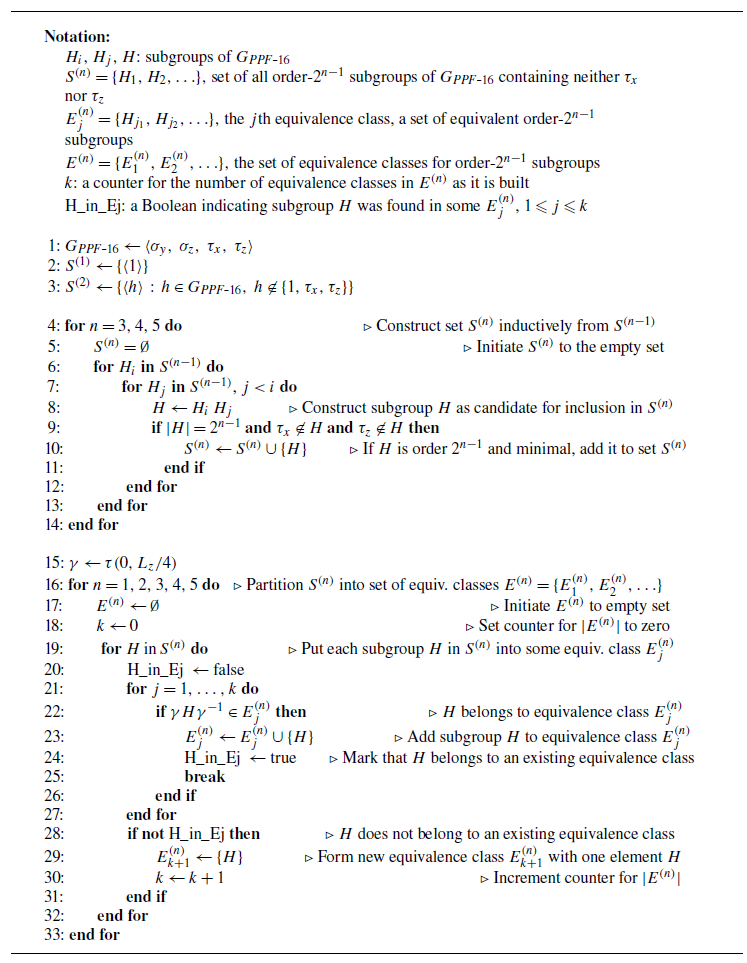
Generate all minimal-domain subgroups of G PPF−16 and arrange into equivalence classes.

Since the number of subgroups and pairwise conjugacies to check is large, we implemented the algorithm described above in symbolic code and generated the subgroups and equivalence classes of
 $G_{\textit{PPF}\hbox{-}16}$
computationally. Our symbolic codes were written in the Julia programming language (Bezanson et al. Reference Bezanson, Edelman, Karpinski and Shah2017); pseudocode for the algorithm is given in Algorithm 1. The action of an arbitrary symmetry
 $\gamma \in G_{\textit{PPF}}$
can be represented by
 \begin{align} \gamma [u,v,w](x,y,z) = [s_x u, s_y v, s_z w](s_x x + a_x L_x, s_y y, s_z z + a_z L_z) ,\end{align}
where
 $a_x, a_z$
are real valued and
 $s_x, s_y, s_z$
take values
 $\pm 1$
. The symbolic code represents a given symmetry
 $\gamma$
by its five-tuple parametrisation
 $(s_x, s_y, s_z, a_x, a_z)$
and computes inverses and group multiplication in terms of this representation. Arithmetic on
 $a_x$
and
 $a_z$
is performed modulo 1 so that each group element has a unique five-tuple representation and equality of group elements can be tested by equality of their five-tuples. The symbolic code uses Julia’s built-in rational number type for
 $a_x, a_z$
rather than floating-point numbers so that group operations and equality tests are exact. The symbolic code represents a group by an array of its group elements. We defined a strict ordering on group elements in terms of the representation, so that a given group has a unique representation and equality of two groups is established by equality of their ordered elements. Conjugation of subgroups
 $\gamma ^{-1} H \gamma$
is performed by conjugation
 $\gamma ^{-1} h \gamma$
of the elements
 $h$
of
 $H$
. Equivalence of subgroups
 $H_1$
and
 $H_2$
under conjugacy by
 $\gamma$
is tested by computing
 $\gamma ^{-1} H_1 \gamma$
and then testing for equality with
 $H_2$
. Group products
 $H_1 H_2$
are determined by pairwise multiplication of all elements of
 $H_1$
against all elements of
 $H_2$
followed by a reduction to a set of sorted, unique elements. Once the parametrisation, group arithmetic and ordering were defined, much of the rest of the functionality of the symbolic code resulted from application of built-in Julia libraries for tuples, arrays, sorting, rational numbers and tests for equality and set membership. To check for correctness, we wrote two symbolic codes independently and confirmed that they produced identical sets of subgroups and conjugacy classes. We also performed manual verification of conjugacy between the subgroups in each equivalence class.
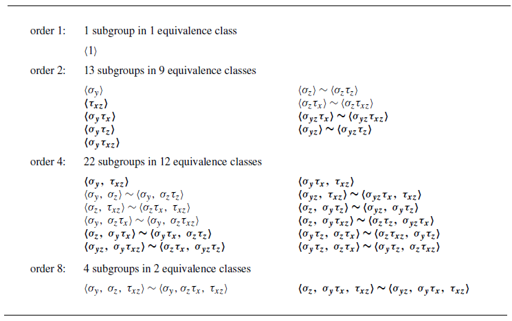
Table 1 provides a complete list of the
 $z$
-centred minimal subgroups of
 $G_{\textit{PPF}}$
with elements of order two or less and their equivalence classes. The subgroups are listed in terms of their generators, e.g.
 $\langle \sigma _y, \tau _{xz} \rangle$
is the fourth-order subgroup
 $\{1, \sigma _y, \tau _{xz}, \sigma _y \tau _{xz}\}$
. The equivalence classes are indicated by equivalence relations between groups, i.e.
 $H_1 \sim H_2$
indicates that groups
 $H_1$
and
 $H_2$
are related by a conjugacy and thus equivalent under a coordinate transformation. A group listed by itself indicates that that group is the sole member of its equivalence class. We find there are 1 order-one subgroups in 1 equivalence class, 13 order-two subgroups in 9 equivalence classes, 22 order-four subgroups in 12 equivalence classes and 4 order-eight subgroups in 2 equivalence classes. Thus there are a total of 24 equivalence classes representing 24 physically distinct symmetry subgroups with second-order elements or less.
Prior studies have found invariant solutions for plane Poiseuille flow in 7 of these 24 distinct subgroups. Waleffe (Reference Waleffe2001) found invariant solutions with
 $\langle \sigma _z\tau _x \rangle$
symmetry. Nagata & Deguchi (Reference Nagata and Deguchi2013) found travelling waves with
 $\langle \sigma _z,\, \tau _{xz} \rangle$
,
 $\langle \sigma _y,\, \sigma _z\tau _{xz} \rangle$
and
 $\langle \sigma _y, \, \sigma _z, \, \tau _{xz} \rangle$
symmetries. Park & Graham (Reference Park and Graham2015) reported invariant solutions in
 $\langle \sigma _y \rangle$
,
 $\langle \sigma _y, \, \sigma _z \rangle$
,
 $\langle \sigma _y, \, \sigma _z, \, \tau _{xz} \rangle$
and the equivalent subgroup
 $\langle \sigma _y, \, \tau _{xz},\, \sigma _z \tau _x \rangle$
. Gibson & Brand (Reference Gibson and Brand2014) reported travelling waves with
 $\langle \sigma _z \tau _x \rangle$
,
 $\langle \sigma _z \rangle$
,
 $\langle \sigma _y, \, \sigma _z \rangle$
,
 $\langle \sigma _y, \, \sigma _z \tau _x \rangle$
,
 $\langle \sigma _z, \, \tau _{xz} \rangle$
and
 $\langle \sigma _y, \, \sigma _z, \, \tau _{xz} \rangle$
symmetries. Zammert & Eckhardt (Reference Zammert and Eckhardt2015) found a travelling wave with
 $\langle \sigma _y, \, \sigma _z, \, \tau _{xz} \rangle$
symmetry. Thus the 7 previously explored subgroups are
 $\langle \sigma _y \rangle ,$
 $\langle \sigma _z \rangle ,$
 $\langle \sigma _z \tau _x \rangle ,$
 $\langle \sigma _y, \, \sigma _z \rangle ,$
 $\langle \sigma _y, \, \sigma _z\tau _x \rangle \sim \langle \sigma _y, \, \sigma _z\tau _{xz} \rangle ,$
 $\langle \sigma _z, \, \tau _{xz} \rangle $
and
 $\langle \sigma _y, \sigma _z, \tau _{xz} \rangle \sim \langle \sigma _y, \, \sigma _z \tau _x, \, \tau _{xz} \rangle$
. Note that our coordinate system is consistent with Waleffe (Reference Waleffe2001), Toh & Itano (Reference Toh and Itano2003) and Park & Graham (Reference Park and Graham2015). The conventions of Nagata & Deguchi (Reference Nagata and Deguchi2013) differ; they have
 $x$
as the streamwise coordinate,
 $y$
as spanwise and
 $z$
as wall normal. Their
 $\varOmega$
,
 $\mathcal{S},$
 $\mathcal{Z}_{y}$
and
 $\mathcal{Z}_{z}$
symmetries correspond to
 $\sigma _{xy} \tau _{xz},$
 $\sigma _z \tau _{xz},$
 $\sigma _z$
and
 $\sigma _y$
, respectively, in our notation.
2.4. Subgroups with higher-order elements: visualisation of examples
In this section we briefly expand on finite subgroups that involve phase shifts by lengths other than
 $L_x/2$
and
 $L_z/2$
(or equivalently, subgroups of
 $G_{\textit{PPF}}$
with elements of order three or more). In principle it is possible to construct and classify all finite subgroups with elements up to some maximal order using the methods presented in §§ 2.1–2.3. This approach, however, quickly becomes impractical due to combinatoric explosion as
 $n$
increases. Instead we present a number examples of subgroups with higher-order elements, illustrate their structure with a visualisation scheme, and infer some general principles. Two examples of subgroups with second-order elements are provided for comparison. In this section, we use domain-normalised notation
 \begin{align} \overline {\tau }(a,b) = \tau (aL_x, bL_z) ,\end{align}
to simplify notation in the important case where the phase shifts are rational multiples of the periodic lengths. A key question is whether a given set of generators generates a minimal- or non-minimal-domain subgroup; i.e. whether an element of domain-normalised form
 $\overline {\tau }(\alpha ,0)$
or
 $\overline {\tau }(0,\beta )$
for some
 $0\lt \alpha \lt 1$
or
 $0\lt \beta \lt 1$
results from some product of the generators.
Figure 2 provides a visualisation of 11 subgroups of the plane Poiseuille symmetry group
 $G_{\textit{PPF}}$
. Given a subgroup
 $H$
specified in terms of its generators, we expand to a set of group elements
 $H = \{h_1, h_2, h_3, \ldots \}$
and then plot each
 $h_i$
in
 $H$
on the
 $a,b$
plane with markers as indicated in the legend. The markers indicate the points in the (domain-normalised)
 $x,z$
plane where the pattern of the velocity field near the origin is repeated, in some cases with the local orientation of the pattern reversed in the
 $y$
and/or
 $z$
directions. Group elements on the
 $a$
or
 $b$
axes are repeated without shading at
 $a=1$
or
 $b=1$
to indicate the periodicity of the domain.
Visualisations of symmetry subgroups of plane Poiseuille flow. Each panel shows a subgroup
 $H$
of the plane Poiseuille symmetry group
 $G_{\textit{PPF}}$
. The subgroup is specified in terms of its generators,
 $H = \langle h_1 \rangle$
or
 $H = \langle h_1, h_2 \rangle$
. The plot is formed by expanding the group to a set of elements
 $H = \{h_1, h_2, h_3, \ldots \}$
and then plotting each
 $h_i$
in
 $H$
on the
 $a,b$
plane using the marker codings indicated in the legend. Group elements on the
 $a$
or
 $b$
axes are repeated without shading at
 $a=1$
or
 $b=1$
to indicate the periodicity of the domain. (a)
 $H_{a} = \langle \overline {\tau }(1/3, 1/3) \rangle$
, (b)
 $H_{b} = \langle \sigma _y \overline {\tau }(1/4, 1/4) \rangle ,$
(c)
 $H_{c} = \langle \overline {\tau }(1/6, 5/6) \rangle$
, (d)
 $H_{d} = \langle \overline {\tau }(1/5, 3/5) \rangle$
, (e)
 $H_{e} \, = \langle \sigma _y \overline {\tau }(1/10, 3/10) \rangle$
, (f)
 $H_{f} = \langle \overline {\tau }(1/2, 2/3) \rangle$
, (g)
 $H_{g} = \langle \sigma _z \overline {\tau }(1/6, 4/7) \rangle$
, (h)
 $H_{h} = \langle \sigma _z \overline {\tau }(1/2, 0) \rangle$
, (i)
 $H_{i} = \langle \sigma _z \overline {\tau }(1/10, 3/10) \rangle$
, (j)
 $H_{j} = \langle \sigma _z \tau _x, \sigma _y \tau _z \rangle = \langle \sigma _z \overline {\tau }(1/2,0),\, \sigma _y \overline {\tau }(0,1/2) \rangle$
, (k)
 $H_{b} = \langle \sigma _z \tau _{xz}, \sigma _y \tau _z \rangle = \langle \sigma _z \overline {\tau }(1/2,1/2),\, \sigma _y \overline {\tau }(0,1/2) \rangle$
.

Figure 2(a) illustrates the minimal-domain subgroup generated by
 $\overline {\tau }(1/3, 1/3)$
, namely
 $H_c = \langle \overline {\tau }(1/3, 1/3) \rangle = \{1, \overline {\tau }(1/3, 1/3), \overline {\tau }(2/3, 2/3)\}$
. Each group element is of form
 $\tau (a,b)$
; thus each is represented by a blue dot along the diagonal of the
 $a,b$
plane. The pattern of dots reflects the threefold diagonal periodicity
 ${\boldsymbol{u}}(x,y,z) = {\boldsymbol{u}}(x+L_x/3,y,z+L_z/3) = {\boldsymbol{u}}(x+2L_x/3,y,z+2L_z/3)$
of velocity fields with this symmetry group. Since
 $H_c$
has no elements of form
 $\overline {\tau }(\alpha ,0)$
or
 $\overline {\tau }(0,\beta )$
for
 $0\lt \beta \lt 1$
or
 $0\lt \alpha \lt 1$
, it is a minimal-domain subgroup. This can be seen directly in the visualisation by the lack of blue dots on the
 $a$
and
 $b$
axes, apart from the origin. In general the group generated by a single diagonal phase shift of form
 $\overline {\tau }(1/n, 1/n)$
is an
 $n$
th-order minimal-domain subgroup with
 $n$
points of symmetry along the
 $x,z$
diagonal of the spatial domain.
Figure 2(b) illustrates the minimal-domain subgroup generated by
 $\sigma _y \overline {\tau }(1/4,1/4)$
, namely
 $H_{b} = \langle \sigma _y \overline {\tau }(1/4,1/4) \rangle = \{1,\, \sigma _y \overline {\tau }(1/4, 1/4),\, \overline {\tau }(1/2, 1/2),\, \sigma _y \overline {\tau }(3/4, 3/4)\}$
. The structure of this group is similar to that of
 $H_{a} = \langle \overline {\tau }(1/3, 1/3) \rangle$
, except the diagonal elements alternate between pure phase shifts and phase shifts with
 $y$
reflection. For this symmetry group, the pattern of a velocity field at the origin is repeated with the same orientation at
 $x,z = L_x/2, L_z/2$
and with inversion of the pattern in
 $y$
locally at
 $x,z = L_x/4, L_z/4$
and
 $3L_x/4, 3L_z/4$
. In general, a subgroup generated by a symmetry of form
 $\sigma _y \overline {\tau }(1/n,1/n)$
is minimal domain and diagonal,
 $n$
th order if
 $n$
is even, and
 $(2n)$
th order if
 $n$
is odd.
Figure 2(c) illustrates the minimal-domain subgroup generated by
 $\overline {\tau }(1/6, 5/6)$
, namely,
 $H_{c} = \{1,\, \overline {\tau }(1/6, 5/6),\, \overline {\tau }(2/6, 4/6),\, \ldots \,, \overline {\tau }(5/6, 1/6)\}.$
In general,
 $\overline {\tau }(1/n, (n-1)/n)$
for natural number
 $n$
generates the
 $n$
th-order minimal-domain subgroup
 \begin{align} &\langle \overline {\tau }(1/n, (n-1)/n) \rangle \nonumber\\&\quad = \{1,\, \overline {\tau }(1/n, (n-1)/n),\, \overline {\tau }(2/n, (n-2)/n),\, \ldots , \overline {\tau }((n-1)/n, 1/n)\}. \end{align}
The
 $h_j = \overline {\tau }(j/n, (n-j)/n)$
structure of the subgroup elements derives from the fact that
 $n-j \equiv -j \mod n$
, by which
 $\overline {\tau }(1/n, (n-1)/n) = \overline {\tau }(1/n, -1/n)$
, and thus
 $\overline {\tau }^j(1/n, (n-1)/n) = \overline {\tau }^j(1/n, -1/n) = \overline {\tau }(j/n, -j/n) = \overline {\tau }(j/n, (n-j)/n)$
. Alternatively, since
 $\overline {\tau }(1/n, (n-1)/n) = \overline {\tau }(1/n, -1/n) = \sigma _z \overline {\tau }(1/n, 1/n) \sigma _z^{-1}$
, one can view the subgroup
 $\langle \overline {\tau }(1/n, (n-1)/n) \rangle$
as equivalent to
 $\langle \overline {\tau }(1/n, 1/n) \rangle$
under conjugacy by
 $\sigma _z$
. Subgroups of this form are minimal domain and
 $n$
th order for all natural numbers
 $n$
, and they induce anti-diagonal structure, with
 $n$
points of symmetry along the diagonal of slope
 $-L_z/L_x$
in the
 $x,z$
plane.
Figure 2(d) illustrates the minimal-domain subgroup generated by the
 $\overline {\tau }(1/5, 3/5)$
, namely
 $H_{d} = \{1,\, \overline {\tau }(1/5, 3/5),\, \overline {\tau }(2/5, 1/5),\, \ldots \,, \overline {\tau }(4/5, 2/5)\}$
. The general form of this type is
 $\overline {\tau }(j/p, k/p)$
for prime
 $p$
and integers
 $j,k$
, satisfying
 $1\lt j,k\lt p$
. This generates a minimal-domain diagonal subgroup similar to
 $\langle \tau (1/n, 1/n) \rangle$
or
 $\langle \tau (1/n, (n-1)/n) \rangle$
, since each of
 $j,k$
are relatively prime to
 $p$
, so that
 $\ell j \!\!\! \mod p \equiv 0$
and
 $\ell k \!\!\! \mod p \equiv 0$
only for the same values of
 $\ell$
, namely multiples of
 $p$
. Note the difference from the subgroups generated by
 $\overline {\tau }(j/n, k/n)$
for non-prime
 $n$
, which are minimal domain only if
 $j$
and
 $k$
are 1 or
 $n-1$
(or an integer congruent to these mod
 $n$
). This difference is related to the fact that the integers mod
 $p$
form a Galois field only when
 $p$
is prime. In general, subgroups of this type induce a diagonal winding pattern in the
 $x,z$
plane of the velocity field.
Figure 2(e) illustrates a minimal-domain subgroup generated by an element of form
 $\sigma _y \overline {\tau }(j/n, k/n)$
for
 $j,k$
relatively prime to natural number
 $n$
. The example shown is
 $H_{e} = \langle \sigma _y \overline {\tau }(1/10, 3/10) \rangle$
. Since
 $(\sigma _y \overline {\tau }(1/10, 3/10))^2 = \overline {\tau }(1/5, 3/5)$
, the generator of example (d), it follows that
 $H_{d}$
is a subgroup of
 $H_{e}$
, and thus the markers for
 $H_{d}$
in (d) are a subset of the markers for
 $H_{e}$
in (e). Velocity fields with
 $H_{e}$
symmetry will have the same diagonal winding structure as in (d), but with additional antinodes of symmetry with reversal of
 $y$
orientation halfway between the nodes of (d).
Figure 2(f) illustrates the non-minimal-domain subgroup generated by
 $\overline {\tau }(1/2, 2/3)$
, namely
 $H_{f} = \langle \overline {\tau }(1/2, 2/3) \rangle = \{1,\, \overline {\tau }(1/2, 2/3),\, \overline {\tau }(0, 1/3),\, \overline {\tau }(1/2, 0), \ldots , \overline {\tau }(1/2, 1/3)\}$
. In contrast to subgroups
 $H_{a}$
through
 $H_{d}$
, this subgroup is non-minimal due to the presence of elements
 $\overline {\tau }^2(1/2, 2/3) = \overline {\tau }(0, 1/3)$
,
 $\overline {\tau }^3(1/2, 2/3) = \overline {\tau }(1/2, 0)$
and
 $\overline {\tau }^4(1/2, 2/3) = \overline {\tau }(0, 2/3)$
, each of which appears in the figure as a blue dot on the
 $a$
or
 $b$
axis away from the origin. The general form of this type is
 $\langle \overline {\tau }(j/m, k/n) \rangle$
, where
 $j/m$
and
 $k/n$
are in rational numbers in reduced form and
 $m,n$
are unequal natural numbers. Such subgroups are non-minimal because the integers modulo a composite number
 $mn$
do not form a Galois field.
Figure 2(i,j) illustrate the simplification of a non-
 $z$
-centred, non-minimal-domain subgroup to
 $z$
-centred, minimal-domain form. Figure 2(g) shows the subgroup
 $H_{g} = \langle \sigma _z \overline {\tau }(1/6, 4/7) \rangle = \{1,\,\,\, \sigma _z \overline {\tau }(1/6, 4/7),\,\,\, \overline {\tau }(1/3, 0),\,\,\, \sigma _z \overline {\tau }(1/2, 4/7),\,\,\, \overline {\tau }(2/3, 0), \sigma _z \overline {\tau }(5/6, 4/7)\}$
. This subgroup is non-
 $z$
-centred since it has elements of the form
 $\sigma _z \overline {\tau }(a,b)$
with
 $b\neq 0$
, but no element of form
 $\sigma _z \overline {\tau }(a,0)$
. The conjugation
 $H_{g}' = \gamma H_{g} \gamma ^{-1}$
for
 $\gamma = \overline {\tau }(0, 2//7)$
, produces an equivalent
 $z$
-centred, non-minimal subgroup
 $H_{g}' = \langle \sigma _z \overline {\tau }(1/6, 0) \rangle = \{1, \sigma _z \overline {\tau }(1/6, 0), \overline {\tau }(1/3, 0), \sigma _z \overline {\tau }(1/2, 0), \overline {\tau }(2/3, 0), \sigma _z \overline {\tau }(5/6, 0)\}$
(not shown). The presence of
 $\overline {\tau }(1/3, 0)$
symmetry in
 $H_{g}$
and
 $H_{g}'$
implies a periodicity of
 $L_x/3$
in
 $x$
, so we further simplify this subgroup by recasting on a domain with this smaller periodicity. This is accomplished by multiplying the
 $x$
component of each normalised phase shift by 3 and simplifying,
 $\sigma _z \overline {\tau }(1/6, 0) \rightarrow \sigma _z \overline {\tau }(1/2, 0)$
and
 $\overline {\tau }(1/3, 0) \rightarrow \overline {\tau }(3/3, 0) = 1$
, etc., resulting in the
 $z$
-centred, minimal-domain subgroup
 $H_{h} = \langle \sigma _z \overline {\tau }(1/2, 0) \rangle = \{1, \sigma _z \overline {\tau }(1/2, 0)\}$
shown in figure 2(h).
Figure 2(i) in comparison with (e) illustrates the substantial difference in the behaviour of
 $z$
- and
 $y$
-reflection symmetries
 $\sigma _z$
and
 $\sigma _y$
in combination with phase shifts
 $\overline {\tau }(a,b)$
. Figure 2(i) shows
 $H_{i} = \langle \sigma _z \overline {\tau }(1/10,3/10) \rangle$
, whose generator differs from that of
 $H_{e} = \langle \sigma _y \overline {\tau }(1/10,3/10) \rangle$
only by the replacement of
 $\sigma _z$
for
 $\sigma _y$
. In contrast to
 $H_{e}$
,
 $H_{i}$
is neither
 $z$
-centred nor minimal domain. It can be simplified to the
 $z$
-centred minimal-domain subgroup
 $H_{h} = \langle \sigma _z \overline {\tau }(1/2, 0) \rangle$
by a process similar to the reduction of
 $H_{g}$
.
Lastly, figure 2(j, k) illustrate two equivalent minimal-domain half-box subgroups
 $H_{j} = \langle \sigma _z \tau _x, \sigma _y \tau _z \rangle$
and
 $H_{k} = \langle \sigma _z \tau _{xz},\, \sigma _y \tau _z \rangle$
. Expanded in domain-normalised notation,
 $H_{j} = \{1,\, \sigma _z \overline {\tau }(1/2, 0),\, \sigma _y \overline {\tau }(0, 1/2), \sigma _{yz} \overline {\tau }(1/2, 1/2)\}$
and
 $H_{k} = \{1,\, \sigma _z \overline {\tau }(1/2, 1/2), \sigma _y \overline {\tau }(0, 1/2),$
 $\sigma _{yz} \overline {\tau }(1/2, 0)\}$
. We note that, for any group element
 $h = \sigma _y^j \sigma _z^k \tau (a,b,)$
and any
 $\gamma \in G_{\textit{PPF}}$
, the conjugacy
 $h' = \gamma h \gamma ^{-1}$
leaves
 $j$
and
 $k$
unchanged. Thus two equivalent subgroups have the same set of symbols in the visualisation, but in different locations on the
 $a,b$
plane. For half-box groups, the locations are restricted to the four points
 $(a,b) \in \{0,1/2\} \times \{0,1/2\}$
, so equivalent half-box groups have the same symbols permuted between these positions.
From these examples we infer and present without proof a few general principles of subgroups with higher-order elements.
-
(i) Any element of
$G_{\textit{PPF}}$
with rational normalised phase shifts has finite order. -
(ii) The subgroup
$H = \langle \overline {\tau }(j/p, k/p) \rangle$
, where
$p$
is prime and
$j,k$
are integers
$1 \leqslant j,k \lt p$
, is finite and has
$p$
elements (
$|H| = p$
). -
(iii) If a subgroup contains a phase shift
$\overline {\tau }(j/m, k/n)$
where
$j/m$
and
$k/n$
are reduced rationals with natural numbers
$m,n$
,
$m\neq n$
and integers
$j,k$
relatively prime to
$m$
and
$n$
, respectively, then the subgroup is non-minimal. -
(iv) A subgroup containing an element
$\sigma _z \overline {\tau }(a,b)$
is minimal only for
$a=0$
or
$1/2$
.


These examples and principles provide some structure for understanding the features of the symmetry subgroups of plane Poiseuille symmetry involving phase shifts other than half the periodic lengths. They also illustrate a rich variety of possible symmetry groups for velocity fields and invariant solutions in a doubly periodic computational domain, and the potential for further classification based on number theory.
3. Nonlinear travelling waves
In this section, we start by outlining the numerical approach and discuss about exploiting connections between imposed symmetries and the dynamics. We also report the fifteen new numerically calculated travelling-wave solutions of plane Poiseuille flow in seven different symmetric subspaces. These solutions differ from those reported in previous studies such as Park & Graham (Reference Park and Graham2015). This can be seen by comparing symmetry properties or the minimum Reynolds numbers at which the solutions go through a saddle-node bifurcation. A summary of the properties is given in table 2. Lastly, we present streamwise-averaged cross-sections and Reynolds-number continuations of the computed travelling waves and discuss their structure and bifurcations.
Properties of numerically calculated travelling waves. Fifteen newly found travelling waves of plane Poiseuille flow are summarised in terms of their periodic domains, wavespeeds and symmetry groups. The wavespeeds
 $c_x, c_z$
, dissipation rate
 $D$
, number of unstable eigenvalues and eigenvalue with maximum real part are reported for the lower branch of the solution at
 ${\textit{Re}}=2000$
. Boldfaced symmetry groups indicate hitherto unexplored invariant spaces.

3.1. Numerical approach
We used Channelflow
 $2.0$
to compute travelling-wave solutions of plane Poiseuille flow on doubly periodic domains in a selection of symmetric subspaces. Channelflow uses the Newton–Krylov–hookstep algorithm of Viswanath (Reference Viswanath2007) to find solutions of (1.6) while enforcing a given symmetry subgroup by projection with its generators, as described in § 1.3. For travelling waves, the invariance equation (1.6) is
 \begin{align} \tau (c_x t, c_z t) \, \phi ^t({\boldsymbol{u}}) - {\boldsymbol{u}} = 0 ,\end{align}
for all
 $t \geqslant 0$
, unknown wavespeeds
 $c_x, c_z$
, and unknown
 $\boldsymbol{u}$
. Channelflow solves the related equation
 \begin{align} \overline {\tau }(a_x, a_z) \, \phi ^T({\boldsymbol{u}}) - {\boldsymbol{u}} = 0 ,\end{align}
where
 $T$
is fixed,
 $\overline {\tau }$
is the domain-normalised form of a phase shift (2.5), and the free variables are the spectral coefficients of
 $\boldsymbol{u}$
and the domain-normalised phase shifts
 $a_x, a_z$
on the periodic unit interval. The computed phase shifts are nominally related to the wavespeeds by
 $c_x = a_x L_x/T, c_z = a_z L_z/T$
. After convergence of a solution we check that the computed values of
 $a_x, a_z$
are on the correct branch of the periodic unit interval and produce the correct wavespeeds by verifying that
 $\tau (c_x t, c_z t) \phi ^t({\boldsymbol{u}}) - {\boldsymbol{u}} = 0$
for
 $0 \lt t \leqslant T$
.
The control parameters for a computation of a travelling wave are the periodic domain lengths
 $L_x, L_z$
, the Reynolds number
 ${\textit{Re}}$
, the fixed integration time
 $T$
and the symmetry group
 $H \leqslant G_{\textit{PPF}}$
. We chose
 ${\textit{Re}} = 2000$
,
 $L_x, L_z = 2\pi , \pi$
or
 $\pi , \pi /2$
and
 $T=5$
. For
 $H$
we selected several of the subgroups derived in § 2.3, namely
 $H = \langle \sigma _y \rangle$
,
 $\langle \sigma _z,\, \tau _{xz} \rangle$
,
 $\langle \sigma _y,\, \tau _{xz} \rangle$
,
 $\langle \sigma _y,\, \sigma _z,\, \tau _{xz} \rangle$
,
 $\langle \sigma _y,\, \sigma _z \rangle$
,
 $\langle \sigma _y,\, \sigma _z\tau _x \rangle$
and
 $\langle \tau (L_x/3, L_z/3)\rangle$
. All numerical computations were performed at the discretisation of
 $N_x \times N_y \times N_z = 48 \times 81 \times 48$
, with dealiasing in periodic directions performed using the 2/3 dealiasing rule. Time marching was done using a third-order semi-implicit backward differentiation scheme. We confirmed the adequate numerical resolution by recomputing each solution at higher resolution of
 $96 \times 97 \times 96$
.
To generate initial guesses, we generated random divergence-free initial conditions
 ${\boldsymbol{u}}(0)$
with exponentially decaying spectral coefficients to mimic the smoothness of transitionally turbulent velocity fields. We projected the random field onto the given symmetric subspace and then rescaled it to have sufficient magnitude to evolve into sustained unsteady flow. We generated time-series data by time integration,
 ${\boldsymbol{u}}(t) = \phi ^t({\boldsymbol{u}}(0))$
, with the symmetry group
 $H$
imposed by periodically projecting with its generators, as discussed in § 1.3. Since travelling waves are moving steady states, initial guesses for the travelling-wave search were selected by scanning the time-series data for states with a close balance of energy input and dissipation rates. Following Toh & Itano (Reference Toh and Itano2003) and Park & Graham (Reference Park and Graham2015) we define these rates as
 \begin{align}I &= \frac {1}{2L_{z}}\int _{0}^{L_{z}}\int _{-1}^{1} ( p_{\textit{tot}}\boldsymbol{u_{\textit{tot}}}|_{x=0} \;-\; p_{\textit{tot}}\boldsymbol{u_{\textit{tot}}}|_{x=L_{x}} ) \; {\rm d}y \, {\rm d}z,\end{align}
 \begin{align}D &= \frac {1}{2 L_{x} L_{z}} \int _{0}^{L_{z}}\int _{-1}^{1} \int _{0}^{L_{x}} \big(|\boldsymbol{\nabla } \boldsymbol{u_{\textit{tot}}}|^{2} + |\boldsymbol{\nabla } v_{\textit{tot}}|^{2} + |\boldsymbol{\nabla } w_{\textit{tot}}|^{2} \big)\; {\rm d}x\, {\rm d}y\, {\rm d}z.\end{align}
We selected initial guesses
 $\hat {\boldsymbol{u}}$
from time-series states
 ${\boldsymbol{u}}(t)$
that satisfied
 $| D - I | \leqslant 2 \times 10^{-3}$
. Guesses
 $\hat {a}_x, \hat {a}_z$
for domain-normalised phase shifts were then obtained by minimising
 $\| \overline {\tau }(\hat {a}_x, \hat {a}_z) \phi ^T(\hat {\boldsymbol{u}}) - \hat {\boldsymbol{u}}\|$
over
 $\hat {a}_x, \hat {a}_z$
in
 $[-1/2, 1/2)$
. We fixed the integration times to
 $T=5$
, which slowed the rate of convergence of the Newton–Krylov iterations, in that it sometimes took more than
 $100$
iterations for the Newton step to converge. However, the large number of iterations was partially counterbalanced by the shorter integration time. For larger values of
 $T$
, we rarely observed any success. We also tried initial guesses from states that lingered around a point in the
 $D$
versus
 $I$
plane for
 $10$
time units or more. Our overall success rate was low: approximately one in ten initial guesses converged to a travelling wave.
As noted in § 1.3, a
 $z$
-reflection symmetry pins the phase of a velocity field to a centre in
 $z$
, thus precluding travelling waves from travelling in
 $z$
and fixing the spanwise wavespeed to
 $c_z=0$
. This property holds for any symmetry subgroup with a generator that has a factor of
 $\sigma _z$
. Let
 $\boldsymbol{u}$
be a travelling-wave solution of (3.1) with symmetry subgroup
 $H$
with generator
 $h = \sigma _y^j \sigma _z \tau (a,b)$
where
 $j =0$
or 1. Since
 $h \in G_{\textit{PPF}}$
it commutes with
 $\phi ^t$
(1.6), so
 \begin{align} h \phi ^t({\boldsymbol{u}}) = \phi ^t(h {\boldsymbol{u}}) ,\end{align}
for all
 $t \geqslant 0$
. From (3.1) we have
 $\phi ^t({\boldsymbol{u}}) = \tau (-c_x t, -c_z t)\, {\boldsymbol{u}}$
. Substituting this and the value of
 $h$
into (3.5) gives
 \begin{align} \sigma _y^j\, \sigma _z\, \tau (a,b)\, \tau (-c_x t, -c_z t)\, {\boldsymbol{u}} &= \tau (-c_x t, -c_z t)\, \sigma _y^j\, \sigma _z\, \tau (a,b)\, {\boldsymbol{u}} \nonumber \\ &= \sigma _y^j\, \sigma _z\, \tau (-c_x t, c_z t)\, \tau (a,b)\, {\boldsymbol{u}}. \end{align}
Multiplying this from the left by
 $\tau (c_x t, c_z t)\, \tau (-a,-b)\, \sigma _z\, \sigma _y^j$
gives
 \begin{align} {\boldsymbol{u}} &= \tau (0, 2c_z t)\, {\boldsymbol{u}} ,\end{align}
for all
 $t \geqslant 0$
. By this equation, either
 $c_z = 0$
or
 $\boldsymbol{u}$
is independent of
 $z$
, in which case
 $c_z$
is arbitrary and can be taken as
 $c_z = 0.$
Thus, if the symmetry subgroup
 $H$
has a generator with a factor of
 $\sigma _z$
, we compute travelling waves by solving (3.1) with
 $a_z=0$
held fixed.
For relative periodic orbits, the spanwise pinning effect is slightly different. The invariance equation (1.6) in this case is
 \begin{align} \tau (\ell _x, \ell _z) \, \phi ^T({\boldsymbol{u}}) - {\boldsymbol{u}} = 0 ,\end{align}
for unknown
 $\ell _x, \ell _z, T$
and
 $\boldsymbol{u}$
, where
 $T \gt 0$
. Let
 $\ell _x, \ell _z, T$
and
 $\boldsymbol{u}$
be a solution of (3.8), and let the symmetry group of
 $\boldsymbol{u}$
have a generator of form
 $h = \sigma _y^j \sigma _z \tau (a,b)$
where
 $j=0$
or 1. From (3.8) we have
 $\phi ^T({\boldsymbol{u}}) = \tau (-\ell _x, -\ell _z) {\boldsymbol{u}}$
. Substituting this and the value of
 $h$
into (3.5) at
 $t=T$
gives
 \begin{align} \sigma _y^j\, \sigma _z\, \tau (a,b)\, \tau (-\ell _x, -\ell _z)\, {\boldsymbol{u}} &= \tau (-\ell _x, -\ell _z)\, \sigma _y^j\, \sigma _z\, \tau (a,b)\, {\boldsymbol{u}} \nonumber \\ &= \sigma _y^j\, \sigma _z\, \tau (-\ell _x, \ell _z t)\, \tau (a,b)\, {\boldsymbol{u}} .\end{align}
Multiplying this from the left by
 $\tau (\ell _x, \ell _z)\, \tau (-a,-b)\, \sigma _z\, \sigma _y^j$
and simplifying gives
 \begin{align} {\boldsymbol{u}} &= \tau (0, 2 \ell _z)\, {\boldsymbol{u}} .\end{align}
If the minimal spanwise periodic length is
 $L_z\gt 0$
, we then have
 $\ell _z=0$
or
 $L_z/2$
. Unlike the travelling-wave case where (3.7) holds for continuous
 $t$
, here, we cannot rule out the non-zero value of the phase shift.
The appearance of a zero spanwise wavespeed in a travelling-wave computation or a spanwise phase shift of
 $L_z/2$
for a relative periodic orbit can be used to deduce a
 $z$
reflection symmetry that was not enforced in the search but instead arose as a property of the solution. For example, the travelling wave
 $\text{P}2$
of Park & Graham (Reference Park and Graham2015) with
 $\sigma _y$
symmetry has spanwise wavespeed
 $c_z=0$
; thus we conjecture that it also has a
 $z$
reflection symmetry of generic form
 $h = \sigma _y^k \sigma _z \tau (a,b)$
, which can be transformed to a
 $z$
-centred symmetry
 $h' = \sigma _y^k \sigma _z \tau (a,0)$
by an appropriate phase shift
 ${\boldsymbol{u}}' = \tau (0,b/2) {\boldsymbol{u}}$
,
 $h' = \tau (0,-b/2) \, h \, \tau (0,b/2)$
following Theorem 1. The appropriate value of
 $b$
can be found numerically, for example, by minimising
 $\| \sigma _y^k \sigma _z \tau (a,b) {\boldsymbol{u}} -{\boldsymbol{u}}\|$
over
 $a,b$
and
 $k=0,1$
. Similarly, a solution computed on a given
 $L_x,L_z$
-periodic domain can exhibit a
 $\tau (a,0)$
or
 $\tau (0,b)$
symmetry for
 $0 \lt a \lt L_x$
,
 $0 \lt b \lt L_z$
, implying periodicity on a smaller domain. This occurred in our computations of
 ${TW}_{9}$
and
 $\textit{TW}_{12}$
and is furthered discussed in § 3.2.
3.2. Nonlinear travelling waves: structures and bifurcations
Table 2 summarises the nonlinear travelling waves we found by the methods of (3.1). Traveling waves
 $\textit{TW}_{1}$
through
 $\textit{TW}_{4}$
were computed for
 $L_x, L_z = \pi , \pi /2$
. All the other solutions were computed for
 $L_x, L_z = 2\pi ,\pi$
. The traveling wave
 $\textit{TW}_{9}$
was computed on this domain but then found to have an unimposed
 $\tau _x = \tau (L_x/2,0)$
symmetry, and was then recast to its minimal
 $\pi \times \pi$
domain. Similarly,
 $\textit{TW}_{12}$
was computed on a
 $2\pi ,\pi$
domain, was found to have
 $\tau _z = \tau (0,L_z/2)$
symmetry, and was recast onto its minimal
 $2\pi , \pi /2$
domain. A striking fact reflected in table 2 is the dominance of streaky flows. Streamwise speeds (
 $c_x$
) are generally orders of magnitude larger than the spanwise speeds (
 $c_z$
) owing to the strong driving streamwise bulk velocity and the streaky flows that result.
Close passes of turbulent trajectories to travelling waves illustrated by the normalised distance
 $\delta (t)$
versus
 $t$
between a turbulent trajectory and the given travelling waves in the (a)
 $\langle \sigma _y \rangle$
, (b)
 $\langle \tau _{xz}, \sigma _z \rangle$
, (c)
 $\langle \tau _{xz}, \sigma _y \rangle$
, (d)
 $\langle \sigma _z, \sigma _y \rangle$
, (e)
 $\langle \sigma _z \tau _x, \sigma _y \rangle$
and (f)
 $\langle \tau (L_x/3, L_z/3)\rangle$
symmetric subspaces. Black dots denote locations of the closest passes to each travelling wave.

To address the dynamical importance of the travelling waves, we calculate the norm of the difference between turbulent trajectories in the invariant subspaces and each of the travelling-wave solutions with the same symmetries. The minimum distance between a field taken from a turbulent trajectory
 ${\boldsymbol{u}}(t)$
and a travelling wave
 ${\boldsymbol{u}}_{\textit{TW}}$
was calculated by optimising over phase shifts in both streamwise and spanwise directions. Modifying the definition of Park & Graham (Reference Park and Graham2015), we denote this distance by
 $\delta (t)$
, defined as follows:
 \begin{equation} \delta (t) = \min _{0 \leqslant a_x,a_z \lt 1} \frac {\|{\boldsymbol{u}}(x+a_xL_x, y, z+a_zL_z, t) - {\boldsymbol{u}}_{\textit{TW}}(x, y,z, t) \|}{\|{\boldsymbol{u}}(t) \|_{\textit{rms}}}, \end{equation}
where
 $\|{\boldsymbol{u}}(t) \|_{\textit{rms}}$
is the root mean square of the norm of velocity fields of the turbulent time series. Figure 3 shows the normalised
 $\delta (t)$
for the computed travelling waves; each panel illustrates close passes to the travelling waves found in the same symmetric subspace. Traveling waves
 $\textit{TW}_{2}$
and
 $\textit{TW}_{9}$
each have an additional symmetry beyond those enforced in the simulation; they are grouped with other travelling waves in the symmetric subspace in which they were found. The magnitude of
 $\delta (t)$
for all close passes was
 $O(10^{-1})$
. The significance of this result is discussed in § 4.1.
Figures 4 and 5 show the streamwise-average velocity fields of the travelling waves and the close passes to them by turbulent trajectories. The close passes reflect the general structure of the travelling waves they approach, in terms of the locations and strengths of mean spanwise
 $v,w$
rolls, but there are notable differences in moderate- to fine-scale structure. The close passes shown in figures 4 and 5 correspond to the black dots in figure 3.
Close passes of turbulent trajectories to
 $\textit{TW}_1$
–
 $\textit{TW}_4$
illustrated by streamwise-averaged
 $y,z$
cross-sections of the velocity fields. Panels show (a)
 $\textit{TW}_{1}$
, (b)
 $\textit{TW}_{2}$
, (c)
 $\textit{TW}_{3}$
, (d)
 $\textit{TW}_{4}$
. In each case the right subplot is the given travelling wave, and the left subplot is the the streamwise-averaged cross-section of the closest pass of the turbulent trajectory, at the point marked with a black dot in figure 3. Arrows indicate cross-stream
 $v,w$
velocity, and the colour map indicates the streamwise velocity
 $u$
.

Close passes of turbulent trajectories to
 $\textit{TW}_7$
–
 $\textit{TW}_{10}$
illustrated by streamwise-averaged
 $y,z$
cross-sections of the velocity fields. Panels show (a)
 $\textit{TW}_{7}$
, (b)
 $\textit{TW}_{8}$
, (c)
 $\textit{TW}_{9}$
, (d)
 $\textit{TW}_{10}$
. In each case the right subplot is the given travelling wave, and the left subplot is the streamwise-averaged cross-section of closest pass of the turbulent trajectory, at the point marked with a black dot in figure 3. Arrows indicate cross-stream
 $v,w$
velocity, and the colour map indicates the streamwise velocity
 $u$
.

Dissipation versus input and continuation curves for
 $\textit{TW}_1$
through
 $\textit{TW}_8$
. (a,c,e) Dissipation
 $D$
versus energy input
 $I$
at
 ${\textit{Re}} = 2000$
. Travelling waves are marked with dots. The dashed line in each case is a typical turbulent trajectory in the given symmetric subspace. (b,d,f) Dissipation
 $D$
versus
 ${\textit{Re}}$
continuation curves of the travelling waves. The enforced symmetry groups for each pair of curves are (a,b)
 $\langle \sigma _y \rangle$
, (c,d)
 $\langle \sigma _z,\, \tau _{xz} \rangle$
, (e,f)
 $\langle \sigma _y,\, \tau _{xz} \rangle$
.

Dissipation versus input and continuation curves for
 $\textit{TW}_9$
through
 $\textit{TW}_{14}$
. (a,c) Dissipation
 $D$
versus energy input
 $I$
at
 ${\textit{Re}} = 2000$
. Travelling waves are marked with dots. The dashed line in each case is a typical turbulent trajectory in the given symmetric subspace. (b,d) Dissipation
 $D$
versus
 ${\textit{Re}}$
continuation curves of the travelling waves. The enforced symmetry groups for each pair of curves are (a,b)
 $\langle \sigma _y,\, \sigma _z \rangle$
(c,d)
 $\langle \sigma _y,\, \sigma _z\tau _x \rangle$
. The traveling wave
 $\textit{TW}_{9}$
has a degeneracy as discussed in § 3.2. At
 ${\textit{Re}} \approx 1273$
(black dot in b),
 $\textit{TW}_{10}$
connects to
 $\textit{TW}_{9}$
in a symmetry-breaking bifurcation. This is followed by another symmetry-breaking bifurcation at
 ${\textit{Re}} \approx 1894$
(red dot). See § 3.2 for further details.

Figures 6 and 7 show energy dissipation versus input for travelling waves and typical turbulent trajectories (left) and continuation curves for travelling waves (right). The dissipation versus versus input curves were computed at
 ${\textit{Re}}=2000$
in the symmetric subspaces and spatial domains in which each travelling wave was found. The dots on the
 $D=I$
lines indicate the dissipation–energy balance of each travelling wave. Each of the travelling waves shown is the lower branch of its continuation curve in Reynolds number shown on the right. It is apparent from the dissipation-input figures that most of these lower-branch travelling waves are embedded in the chaotic sets of the turbulent trajectories.
Figure 7(b) shows a bifurcation of
 $\textit{TW}_{10}$
from
 $\textit{TW}_{9}$
at
 ${\textit{Re}} \approx 1273$
, marked by a black dot in the figure. We found both these solutions in a search for travelling waves with
 $\langle \sigma _y, \sigma _z\rangle$
symmetry on a
 $L_x, L_z = 2\pi , \pi$
computational domain. After convergence
 $\textit{TW}_{9}$
was found to have additional symmetries and the full symmetry group
 $\langle \sigma _y, \sigma _z, \tau (L_x/4, L_z/2)\rangle$
. The
 $\tau (L_x/4, L_z/2)$
symmetry implies
 $\tau _x = (\tau (L_x/4, L_z/2))^2$
symmetry as well, and thus
 $\textit{TW}_{9}$
is periodic on the half-domain
 $L_x/2, L_z = \pi , \pi$
, as reported in table 2. The
 $\tau (L_x/4, L_z/2)$
symmetry on the full domain is equivalent to
 $\tau _{xz}$
-symmetry on the half-domain. The bifurcation at
 ${\textit{Re}} \approx 1273$
is a symmetry-breaking bifurcation in which
 $\textit{TW}_9$
loses it
 $\tau _{xz}$
-symmetry on the half-domain and
 $\textit{TW}_{10}$
is born with
 $\langle \sigma _y, \sigma _z\rangle$
symmetry on the half-domain and
 $\langle \sigma _y, \sigma _z, \tau _x \rangle$
symmetry on the computational domain. Another symmetry-breaking bifurcation occurs at
 ${\textit{Re}} \approx 1894$
(red dot in figure 7
b), where
 $\tau _x$
symmetry is broken and the new solution has symmetry group
 $\langle \sigma _y, \sigma _z\rangle$
.
The traveling wave
 $\textit{TW}_{12}$
was computed on domain
 $L_x, L_z = 2\pi , \pi$
with imposed symmetries
 $\langle \sigma _z \tau _x, \sigma _y \rangle$
. The converged solution found to have an additional
 $\tau _z$
symmetry and symmetry group
 $\langle \tau _z, \sigma _z \tau _x, \sigma _y \rangle$
. After recasting on the half-domain
 $L_x, L_z = 2\pi , \pi /2$
implied by the
 $\tau _z$
symmetry,
 $\textit{TW}_{12}$
has symmetry group
 $\langle \sigma _z \tau _x, \sigma _y \rangle$
.
3.3. A travelling wave with
$\langle \tau (L_x/3, L_z/3)\rangle$
symmetry

Although we primarily focused on finite subgroups of plane Poiseuille flow with second-order elements and half-box shifts, it is also possible to compute invariant solutions with symmetry groups involving higher-order elements and non-half-box shifts. One such non-trivial, non-half-box shift symmetry group is
 $\langle \tau (L_x/3, L_z/3)\rangle$
. We found one travelling wave with this symmetry group,
 $\textit{TW}_{15}$
, listed in table 2. With no
 $z$
reflection symmetry, this solution has non-zero streamwise and spanwise wavespeeds. The streamwise-averaged
 $y,z$
cross-section and continuation in Reynolds number for
 $\textit{TW}_{\!15}$
are shown in figure 8.
Streamwise-average velocity and continuation in Reynolds number for
 $\langle \tau (L_x/3, L_z/3) \rangle$
-symmetric travelling wave
 $\textit{TW}_{15}$
. (a) The streamwise-averaged
 $y,z$
cross-section of
 $\textit{TW}_{15}$
at
 ${\textit{Re}}=2000$
. Arrows indicate cross-stream
 $v,w$
velocity. The colour map indicates streamwise velocity
 $u$
. (b) Continuation
 $\textit{TW}_{15}$
in Reynolds number.

4. Discussion
4.1. Linearised dynamics and the trust-region radius
A key aim of the study of invariant solutions is to model the dynamics of transitionally turbulent flows in terms of the invariant solutions. One might model transitionally turbulent dynamics as a set of finite-time hops between the neighbourhoods of invariant solutions, governed by the linearisation of the solutions’ finite-time dynamics. The results of this study, however, suggest that a much denser set of solutions is required for this approach. Close passes between turbulent trajectories and travelling waves in the same symmetric subspaces were observed to be
 $O(10^{-1})$
in root-mean-square normalised magnitude and
 $O(10^{-2})$
in unnormalised magnitude. This length scale is significantly larger than the range of accuracy of the linearised finite-time dynamics
 $\phi ^T({\boldsymbol{u}} + \Delta {\boldsymbol{u}}) \approx \phi ^T({\boldsymbol{u}}) + D\phi ^T \Delta {\boldsymbol{u}}$
estimated during the Newton–hookstep search. For each step
 ${\boldsymbol{u}} \rightarrow {\boldsymbol{u}}+\Delta {\boldsymbol{u}}$
, the Newton–hookstep algorithm computes the Newton step
 $\Delta {\boldsymbol{u}}_N$
using the linearised dynamics and estimates the trust-region radius
 $\delta _{\textit{TR}}$
within which the linearisation is accurate. If the Newton step is within the trust region,
 $\|\Delta {\boldsymbol{u}}_N\| \leqslant \delta _{\textit{TR}}$
, the algorithm takes the Newton step,
 ${\boldsymbol{u}} \rightarrow {\boldsymbol{u}}+\Delta {\boldsymbol{u}}_N$
. If
 $\|\Delta {\boldsymbol{u}}_N\| \gt \delta _{\textit{TR}}$
, the algorithm computes the optimal hookstep
 $\Delta {\boldsymbol{u}}_H$
within the trust region and takes the hookstep,
 ${\boldsymbol{u}} \rightarrow {\boldsymbol{u}}+\Delta {\boldsymbol{u}}_H$
. A typical search takes several slowly converging hooksteps until the estimated solution is within the trust region, at which point the algorithm switches to Newton steps and converges quickly. Thus the trust-region radius
 $\delta _{\textit{TR}}$
at which the search switches from hooksteps to Newton steps can be taken as an estimate of the radius of validity of the linearisation of the dynamics about the converged solution. The searches for the travelling waves in § 3 showed that this radius is typically
 $\delta _{\textit{TR}} \sim O(10^{-3})$
and sometimes
 $O(10^{-4})$
, significantly smaller than the
 $\delta = O(10^{-2})$
unnormalised closest passes of turbulent trajectories to the travelling waves. This suggests that a much denser set of travelling waves would need to be computed in order to model turbulent trajectories with the linearised dynamics of the travelling waves they shadow.
4.2. Implications for the study of transitional turbulence
Our study of the plane Poiseuille symmetry subgroups was motivated by their importance in computing invariant solutions: for enumerating the different symmetry subgroups in which to seek invariant solutions, for specifying which kind of solutions each subgroups allows, and for increasing the efficiency of numerical searches. However, knowledge of the symmetry subgroups has application beyond the computation of invariant solutions. As discussed in § 1, the subgroups of
 $G_{\textit{PPF}}$
divide the space of all solutions of the flow into different invariant symmetric subspaces. The dynamics of transitional or turbulent flow in each these subspaces can be studied as independent dynamical systems with independent but presumably related dynamical properties. Small, doubly periodic boxes have been studied as ‘minimal flow units’ for plane Poiseuille and plane Couette flow since Jiménez & Moin (Reference Jiménez and Moin1991) and Hamilton, Kim & Waleffe (Reference Hamilton, Kim and Waleffe1995), addressing such questions as: (i) What is the minimal domain size and Reynolds number that sustains unsteady flow? (ii) What dynamical processes sustain unsteady flow (e.g. Waleffe’s self-sustaining process)? (iii) Can the statistics of turbulence in large-aspect-ratio domains be replicated in small periodic boxes? (iv) What are the minimal perturbations to laminar flow that trigger turbulence? (v) What are the dynamical pathways by which transitional turbulence collapses to laminar flow? Each of these questions can be addressed within the context of a specific symmetry subgroup, and the symmetry-specific answers may well shed light on the dynamics of general unsteady flows, both individually and by comparison. For example, if we find that the
 $\langle \sigma _y, \tau _{xz} \rangle$
subspace requires a much higher Reynolds number to sustain turbulence than the
 $\langle \sigma _y, \sigma _z \rangle$
subspace for a fixed domain size, what does this symmetry-dependent behaviour tell us about the the mechanisms by which transitional turbulence is triggered and kept from relaminarising? Or, if we find that the statistics of one subspace closely replicate those of the general flow while another’s statistics differ markedly, does it mean that transitional turbulence is dominated by structures with the former symmetries and not the latter?
The study of invariant solutions is motivated by the hope of addressing such questions precisely from a dynamical-systems perspective, with well-resolved, time-dependent dynamic processes, rather than time or ensemble averages and approximations to the equations of motion. From this perspective, we reframe the above questions in the context of symmetry, as follows. For each distinct symmetry subgroup of plane Poiseuille flow, plane Couette flow or pipe flow: (vi) What is the minimal Reynolds number that sustains transitional turbulence flow on a given domain? (vii) What domain supports transitional turbulence at the lowest Reynolds number? (viii) What is the lowest-Reynolds-number value of
 $(L_x, L_z, {\textit{Re}})$
for which travelling waves or equilibria exist? For periodic or relative periodic orbit solutions? For edge states? (ix) What are the physical mechanisms corresponding to the quantitative force balance in the lowest-Reynolds-number invariant solutions i.e. what is the minimal self-sustaining process for each symmetry subgroup? (x) Which invariant solutions best replicate the statistics of transitional turbulence with no symmetries, or of transitional flow with the given symmetries? (xi) Can the dynamics of transitional turbulence be understood as a chaotic walk among the set of unstable invariant solutions within the network of their low-dimensional unstable manifolds?
The furthest explorations of these questions have been in the context the
 $\langle \sigma _z \tau _x, \sigma _{xyz} \tau _z \rangle$
-symmetric subspace of plane Couette flow, which contains the Nagata equilibrium (Nagata Reference Nagata1990), Waleffe’s self-sustaining process (Waleffe Reference Waleffe1997) and the periodic orbits and state-space visualisations of (Gibson et al. Reference Gibson, Halcrow and Cvitanović2008, Reference Gibson, Halcrow and Cvitanović2009). In this study, we attempted to find travelling waves for plane Poiseuille flow in a few symmetry subgroups other than those presented in table 2 at similar Reynolds numbers and domains, and found that it was difficult to generate sustained transitional turbulence for some subgroups (see figure 9). For some symmetry subgroups, perturbations of even large magnitude decayed quickly to laminar flow. The questions above arise from these observations of the strong influence of symmetry on the basin of attractions of laminar and turbulent flow in small doubly periodic domains.
Sustained turbulence versus decay to laminar flow in two different symmetric subspaces of plane Poiseuille flow. Each figure shows the
 $L^2$
norm of the fluctuating velocity field
 $\|{\boldsymbol{u}}(t)\|$
as a function of time for ten random initial conditions of magnitude
 $\|{\boldsymbol{u}}(0)\| = 0.1$
. In (a), of ten initial conditions and time integrations with
 $\langle \sigma _y, \sigma _z \rangle$
symmetry, six sustain turbulence for several thousand outer time units and four decay relatively quickly to laminar flow. In (b), of ten similar simulations with
 $\langle \sigma _{yz}, \sigma _y\tau _{xz} \rangle$
symmetry, all initial conditions decay to laminar flow by
 $t=4000$
. The apparently random departures to the laminar solution from unsteady flow suggest that for these parameters and symmetry, turbulence is a chaotic repellor. Simulations were performed at
 ${\textit{Re}}=2000$
in a doubly periodic domain of size
 $L_x, L_z = 2\pi , \pi$
, with a
 $48 \times 81 \times 48$
spatial discretisation with 2/3-style dealiasing.

Another line of inquiry stems from the relations between periodic patterns and patches of turbulent flow within a laminar background. Some doubly periodic solutions have related spanwise-localised forms (Schneider, Gibson & Burke Reference Schneider, Gibson and Burke2010; Gibson & Brand Reference Gibson and Brand2014). Are there other doubly periodic solutions in different symmetry groups that can also be localised? So far there is little success in understanding localisation of periodic solutions through modulation and amplitude equations derived from the Navier–Stokes equations. Perhaps this problem is more tractable in a less-explored symmetry subgroup.
4.3. Extension to higher-order group elements and tilted domains
Our analysis of the subgroups of
 $G_{\textit{PPF}}$
is complete only up to subgroups with second-order elements. Some examples of subgroups with order-three and higher elements are presented in § 2.4, along with some preliminary principles for their organisation. Extending the classification results of this paper to groups with
 $n$
th-order elements would be a matter of group theory and number theory. Extension to doubly periodic domains tilted with respect to the mean pressure gradient or bulk-velocity constraint is also possible. This would especially be applicable in the case of transitional turbulence in large domains, where alternating laminar and turbulent structure align themselves at a particular angle with respect to the streamwise direction (see Tuckerman & Barkley Reference Tuckerman and Barkley2011; Tuckerman et al. Reference Tuckerman, Kreilos, Schrobsdorff, Schneider and Gibson2014). In this case
 $\sigma _z$
is no longer a symmetry of the equations of motion, so a classification of plane Poiseuille subgroups can be arrived at simply by dropping subgroups containing
 $\sigma _z$
as an element or as a factor of an element. In plane Couette flow, one can preserve the tilt in the
 $x,z$
plane by inversion in both
 $x$
and
 $z$
, so the symmetry subgroups of the tilted dynamics allow elements containing the product
 $\sigma _{xz} = \sigma _x\sigma _z$
, but not
 $\sigma _z$
or
 $\sigma _x$
individually.
5. Conclusion
This article analysed subgroups of the symmetry group of plane Poiseuille flow in doubly periodic domains, focusing mainly on subgroups generated by spanwise and wall-normal reflections and streamwise and spanwise half-box shifts. We enumerated the set of subgroups generated by these symmetries and classified them in equivalence classes related by conjugacies. This procedure is general and can be used to classify symmetry subgroups of other parallel shear flows. We recomputed, verified and extended previous analysis of the symmetry subgroups of plane Couette flow (see Appendix B). We presented some examples of groups with phase shifts other than half the periodic length and inferred some general principles of subgroups with higher-order elements.
The interplay between symmetries and dynamics was explained and exploited to find
 $14$
new travelling waves in a variety of symmetry subgroups. Traveling waves
 $\textit{TW}_{1-4}$
and
 $\textit{TW}_{7, 8}$
were shown to travel in both streamwise and spanwise directions, consistent with the imposed symmetries. The spanwise wavespeeds (
 $c_z$
) were found to be smaller by orders of magnitude than the streamwise wavespeeds (
 $c_x$
). This observation is consistent with the streakiness of plane Poiseuille flow, in which perturbation velocities are dominated by streaks in the streamwise direction of the forcing. This could also be due to the streamwise-dominant advection from the mean streamwise flow. To the best of our knowledge, these solutions are first of their kind for plane Poiseuille flow, since all the previously reported travelling waves for this flow configuration travel only in the streamwise direction (note: travelling waves identified by Paranjape, Duguet & Hof (Reference Paranjape, Duguet and Hof2020) do travel in the spanwise direction as well, but those are for a domain tilted with respect to the mean flow.). Based on behaviour of the solution and knowledge of symmetries we conjecture that
 $\text{P}2$
of Park & Graham (Reference Park and Graham2015) has
 $\sigma _z$
or
 $\sigma _z \tau _x$
symmetry in addition to
 $\sigma _y$
symmetry. We also computed one travelling wave in a non-half-box symmetry group
 $\langle \tau (L_x/3, \, L_z/3) \rangle$
.
The complete analysis of half-box subgroups and examples of non-half-box symmetry subgroups suggest a rich variety of physically distinct symmetric subspaces, each with different dynamical behaviour for small domains and transitional Reynolds numbers. We pose a number of questions about the interplay between symmetry and large-amplitude dynamics of transitional turbulence in plane Poiseuille, plane Couette and pipe flow, and what kind of minimal self-sustaining process each symmetry subgroup supports. In addition to these directions for future work, we note that the doubling of the convergence rate obtained by enforcing a second-order symmetry during Krylov iteration will change when the symmetries enforced are third order or higher. Understanding the increased convergence rate for higher-order symmetries is non-trivial and will likely be related to the isotypic decomposition of the space restricted to the symmetry group of interest. Recent work by Rudge & McKenzie (Reference Rudge and McKenzie2024) explained the usage of crystallographic notation for fluid dynamics and should prove useful in further analysis of the symmetries of wall–bounded, transitional shear flows.
Funding
This work was partially supported by the National Science Foundation under NSF CBET Award No. 1554149. Computations were performed on Marvin, a Cray CS500 supercomputer at UNH supported by the NSF MRI program under grant AGS-1919310.
Declaration of interest
Authors report no conflicts of interest.
Appendix A. Conjugacy of subgroups of
$\boldsymbol{G}_{\textit{PPF}\hbox{-}\boldsymbol{16}}$

To determine the equivalence classes of subgroups of
 $G_{\textit{PPF}\hbox{-}16} = \langle \sigma _y, \sigma _z,\tau _x,\tau _z\rangle$
(2.3), we need to determine if two unequal subgroups
 $H$
and
 $H'$
are conjugate, i.e. if
 $H' = \gamma H \gamma ^{-1}$
for some
 $\gamma \in G_{\textit{PPF}}$
. A search for such
 $\gamma$
over its general form
 $\gamma = \sigma _y^j \sigma _z^k \tau (a,b)$
would require a search over
 $j,k \in \{0,1\}$
,
 $a \in [0, L_x)$
and
 $b \in [0, L_z)$
. However, the following theorem shows that we need only to check the single value
 $\gamma = \tau (0, L_z/4)$
.
Theorem 4.
Let
 $H, H'$
be unequal but equivalent subgroups of
 $G_{\textit{PPF}\hbox{-}16}$
. Then
 $H$
and
 $H'$
are conjugate under
 $\gamma = \tau (0,L_z/4)$
.
Proof.
Let
 $H', H$
be unequal, equivalent subgroups of
 $G_{\textit{PPF}\hbox{-}16}$
. Then
 $H' = \gamma H \gamma ^{-1}$
for some
 $\gamma \in G_{\textit{PPF}}$
,
 $\gamma \neq 1$
. The element
 $\gamma$
can be expressed as
 $\gamma = \sigma _y^j \sigma _z^k \tau (a,0) \tau (0,b)$
for some
 $j,k \in \{0,1\}$
and
 $a \in [0, L_x), \, b \in [0, L_z)$
. Since
 $H$
is a subgroup of
 $G_{\textit{PPF}\hbox{-}16}$
, each of its elements can be expressed in form
 $h = \sigma _y^m \sigma _z^n \tau _x^p \tau _z^q$
for some
 $m, n, p, q$
each either 0 or 1. The elements
 $h'$
of
 $H'$
are then given by
 $h' = \gamma h \, \gamma ^{-1}$
for
 $h \in H$
. Substitution gives
 \begin{align} h' &= \big(\tau (a,0)\, \tau (0,b)\, \sigma _y^j \sigma _z^k \big)\, \big(\sigma _y^m\, \sigma _z^n\, \tau _x^p\, \tau _z^q \big)\, \big(\sigma _z^{-k}\, \sigma _y^{-j} \, \tau (-a,0)\, \tau (0,-b) \big). \end{align}
Since the elements
 $\sigma _y, \sigma _z, \tau _x, \tau _z,$
and
 $\tau (\pm a,0)$
commute, we can rearrange these factors and simplify with
 $ \tau (a,0) \tau (-a,0) = \sigma _y^{j} \sigma _y^{-j} = \sigma _z^{k} \sigma _z^{-k} = 1$
, yielding
 \begin{align} h' &= \tau (0,b)\, \sigma _y^m\, \sigma _z^{n}\, \tau _x^{p}\, \tau _z^{q}\, \tau (0,-b). \end{align}
Since
 $\tau (0,-b)$
commutes with
 $\sigma _y, \tau _x,$
and
 $\tau _z$
, but
 $\tau (0,-b)\, \sigma _z^{n} = \tau (0, -(-1)^{n}b) = \tau (0, (-1)^{n+1}b)$
, we have
 \begin{align} h' &= \tau (0,(1+(-1)^{n+1})b) \, \sigma _y^{m}\, \sigma _z^{n}\, \tau _x^{p}\, \tau _z^{q}. \end{align}
There must be at least one
 $h$
in
 $H$
for which
 $\tau (0,(1+(-1)^{n+1})b)$
is not the identity, since the contrary assumption leads to
 $h' = \sigma _y^m\, \sigma _z^n\, \tau _x^p\, \tau _z^q\ = h$
for all
 $h$
in
 $H$
, and thus
 $H' = H$
, which contradicts the assumption
 $H' \neq H$
.
Thus we have
 $n_j = 1$
for some
 $h_j$
in
 $H$
, and
 $h'_j$
has the form
 \begin{align} h'_j = \tau (0, 2b)\, \sigma _y^{m_j}\, \sigma _z^{n_j}\, \tau _x^{p_j}\, \tau _z^{q_j}, \end{align}
where
 $\tau (0,2b) \neq 1$
. Since
 $h'_j$
is an element of a subgroup of
 $G_{\textit{PPF}\hbox{-}16}$
, it is a product of factors
 $\sigma _y, \sigma _z, \tau _x,$
and
 $\tau _z.$
It follows then from (A4) that
 $\tau (0,2b) = \tau _z = \tau (0, L_z/2)$
and thus
 $2b = L_z/2$
. The only values of
 $b$
in the periodic domain
 $[0, L_z)$
that satisfy this equality are
 $b=L_z/4$
and
 $b=3L_z/4$
.
If
 $b=L_z/4$
then substituting this value and
 $h = \sigma _y^m\, \sigma _z^n\, \tau _x^p\, \tau _z^q$
into (A2) gives
 $h' = \tau (0, L_z/4)\, h\, \tau (0, -L_z/4)$
for all
 $h$
in
 $H$
, and thus
 $H'$
is conjugate to
 $H$
under
 $\gamma = \tau (0,L_z/4)$
. If
 $b=3L_z/4$
, then we write
 $\tau (0, \pm 3L_z/4) = \tau (0, \pm L_z/4) \tau (0, \pm L_z/2) = \tau (0, \pm L_z/4) \tau _z$
and substitute into (A2), giving
 \begin{align} h' &= \tau (0,L_z/4)\, \tau _z\, \sigma _y^m\, \sigma _z^n\, \tau _x^p\, \tau _z^q\, \tau (0,-L_z/4)\, \tau _z. \end{align}
Since
 $\tau _z$
commutes with
 $\sigma _y, \sigma _z, \tau _x, \tau _z,$
and
 $\tau (0, \pm L_z/4)$
, this can be reduced to
 $h' = \tau (0,L_z/4)\, \sigma _y^m\, \sigma _z^n\, \tau _x^p\, \tau _z^q\, \tau (0,-L_z/4) = \tau (0, L_z/4)\, h\, \tau (0,-L_z/4)$
, for all
 $h$
in
 $H$
. Thus
 $H'$
is conjugate to
 $H$
under
 $\gamma = \tau (0,L_z/4)$
.
Appendix B. Symmetry subgroups and equivalence classes for plane Couette flow
To verify the symbolic code, we calculated the equivalence classes of symmetry subgroups for plane Couette flow and compared them with Gibson et al. (Reference Gibson, Halcrow and Cvitanović2009). The results, presented in table 3, are for symmetries acting on the fluctuating velocity
 ${\boldsymbol{u}}(x,t)$
of plane Couette flow after a decomposition of total velocity and pressure into a laminar base flow and fluctuation
 ${\boldsymbol{u}}(x,t)$
following Gibson et al. (Reference Gibson, Halcrow and Cvitanović2009), namely
 $\boldsymbol{u_{\textit{tot}}}({\boldsymbol{x}},t) = y {\boldsymbol{e}}_x + {\boldsymbol{u}}({\boldsymbol{x}}, t)$
. This results in Dirichlet boundary conditions on
 $\boldsymbol{u}$
at the walls
 $y = \pm 1$
and renders the space of
 $\boldsymbol{u}$
a vector space. The plane Couette symmetry group
 $G_{\text{PCF}}$
corresponding to
 $G_{\textit{PPF}}$
(1.9) for plane Poiseuille flow is
 \begin{align} G_{\textit{PCF}} = \langle \sigma _{xy},\, \sigma _z,\, \{\tau (a, {b}) \; : \; a,b \in \mathbb{R} \} \rangle , \end{align}
and the 16th-order abelian subgroup of
 $G_{\text{PCF}}$
limited to
 $z$
-centred, half-box phase shifts corresponding to
 $G_{\textit{PPF}\hbox{-}16}$
(2.3) is
Symmetry subgroups and their equivalence classes for plane Couette flow in minimal doubly periodic domains. The symbol
 $\sim$
denotes equivalence between subgroups under conjugation. A set of subgroups related by
 $\sim$
symbols forms an equivalence class. A subgroup listed in isolation forms an equivalence class with that subgroup as its sole element. The first subgroup listed in each equivalence class is chosen as the representative for that equivalence class. The subgroups listed are the complete set of
 $z$
-centred, minimal-domain subgroups with elements of order two or less for plane Couette flow in doubly periodic domains. See § 2.3 for related discussion.

 \begin{align} G_{\textit{PCF-}16} = \langle \sigma _{xy},\, \sigma _z,\, \tau _x, \tau _z \rangle . \end{align}
Table 3 lists the subgroups of
 $G_{\textit{PCF-}16}$
and their equivalence classes. The inversion of the
 $x$
coordinate by
 $\sigma _{xy}$
in
 $G_{\text{PCF}}$
and
 $G_{\textit{PCF-}16}$
, compared with
 $\sigma _y$
in
 $G_{\textit{PPF}}$
and
 $G_{\textit{PPF}\hbox{-}16}$
, means that plane Couette symmetries have the non-commuting product
 $\sigma _{xy} \tau (a,b) = \tau (-a,b) \sigma _{xy}$
in addition to
 $\sigma _z \tau (a,b) = \tau (a,-b) \sigma _z$
. This additional instance of non-abelian behaviour expands the set of elements of
 $\gamma \in G_{\text{PCF}}$
for which conjugacies
 $H' = \gamma H \gamma ^{-1}$
are non-trivial and thereby reduces the total number of equivalence classes from
 $24$
for plane Poiseuille flow to
 $14$
for plane Couette flow. The results agree with Gibson et al. (Reference Gibson, Halcrow and Cvitanović2009) and expand upon them, since Gibson et al. (Reference Gibson, Halcrow and Cvitanović2009) excluded subgroups with isolated
 $\tau _{xz}$
symmetry. Note that Gibson et al. (Reference Gibson, Halcrow and Cvitanović2009) used notation ‘
 $\sigma _x\!$
’ for
 $\sigma _{xy}$
. Daly et al. (Reference Daly, Schneider, Schlatter and Peake2014) showed that rotating plane Couette flow, with a uniform rotation about the spanwise direction, obeys the same symmetries.