1 Introduction
Double diffusive convection (DDC) is the convection flow where fluid density depends on two scalar fields. One of the most relevant applications is oceanic mixing, in which the two scalars are temperature and salinity. Temperature diffuses about 100 times faster than salinity, and this huge difference in the molecular diffusivities allows for very rich dynamics in oceanic DDC flow (Schmitt Reference Schmitt1994). For instance, an instability can occur even when the fluid is overall stably stratified (Stern Reference Stern1960). A comprehensive review of the field can be found in the recent book by Radko (Reference Radko2013).
One of the interesting phenomena in DDC is the salt-finger structure, i.e. narrow elongated vertical flows which were observed in many experiments (e.g. by Turner Reference Turner1967; Linden Reference Linden1978; Taylor & Bucens Reference Taylor and Bucens1989). For a DDC flow bounded by two reservoirs with fixed values for the two scalars, Krishnamurti (Reference Krishnamurti2003, Reference Krishnamurti2009) observed either a single layer of salt fingers, or an alternating stack of salt-finger and convective layers which resembles the thermohaline staircase observed in the ocean (e.g. Tait & Howe Reference Tait and Howe1971; Schmitt et al. Reference Schmitt, Ledwell, Montgomery, Polzin and Toole2005). Three-dimensional direct numerical simulations (DNS) in a fully periodic domain produced layered structures which were very similar to the thermohaline staircase (Stellmach et al. Reference Stellmach, Traxler, Garaud, Brummell and Radko2011; Radko et al. Reference Radko, Flanagan, Stellmach and Timmermans2014). Numerical studies also revealed that internal gravity waves can spontaneously develop through collective instability and modulate the salt-finger field (Stern, Radko & Simeonov Reference Stern, Radko and Simeonov2001; Stellmach et al. Reference Stellmach, Traxler, Garaud, Brummell and Radko2011). In recent DDC experiments by using electrodeposition cells, which are very close to the Rayleigh–Bénard (RB) set-up, Tilgner and coworkers discovered that salt fingers also occur when the fluid is unstably stratified (Hage & Tilgner Reference Hage and Tilgner2010; Kellner & Tilgner Reference Kellner and Tilgner2014). This finding is very surprising and unexpected since one would assume that RB convection dominates in an unstably stratified system. However, linear instability analysis revealed that, in this new regime, salt-finger solutions can indeed be obtained (Schmitt Reference Schmitt2011). Our previous numerical results with the same flow set-up well agreed with those experiments (Yang et al. Reference Yang, van der Poel, Ostilla-Mónico, Sun, Verzicco, Grossmann and Lohse2015).
Numerous theories and models have been developed in the past to understand the scalar fluxes produced by the salt-finger structures, e.g. see Kunze (Reference Kunze2003) and the references therein. Recently, new models were proposed for the fully periodic DDC flow and tested against numerical results, such as the mean-field theory of Traxler et al. (Reference Traxler, Stellmach, Garaud, Radko and Brummell2011) and the equilibrium model of Radko & Smith (Reference Radko and Smith2012). For a finger layer bounded by two solid boundaries, we discovered that the Grossmann–Lohse (GL) theory, which was originally developed for RB flow and showed great success (Grossmann & Lohse Reference Grossmann and Lohse2000, Reference Grossmann and Lohse2001, Reference Grossmann and Lohse2002, Reference Grossmann and Lohse2004; Ahlers, Grossmann & Lohse Reference Ahlers, Grossmann and Lohse2009; Stevens et al. Reference Stevens, van der Poel, Grossmann and Lohse2013), can be directly applied to DDC flow and accurately predicts the salinity flux for both our numerical results (Yang et al. Reference Yang, van der Poel, Ostilla-Mónico, Sun, Verzicco, Grossmann and Lohse2015) and the experimental results (Hage & Tilgner Reference Hage and Tilgner2010).
Although we demonstrated the success of the GL theory in accurately predicting the salinity transfer rate, the behaviour of the flow velocity was not fully investigated in the previous work (Yang et al. Reference Yang, van der Poel, Ostilla-Mónico, Sun, Verzicco, Grossmann and Lohse2015), partially due to the limited control parameters simulated therein. Here, with the help of more systematic simulations which cover a much wider parameter range, we will establish a complete description of the scaling laws for three important global responses, i.e. the salinity and heat transfer rates and the flow velocity. Moreover, we will also investigate the flow structures, such as the salt fingers and the boundary layers. The characteristic length scales of those structures and their dependences on the flow parameters will be discussed.
The paper is organised as follows. We first briefly describe the numerical methods and the parameter space explored (§ 2). In § 3 we develop the scaling laws for the system responses. In § 4 the flow structures and further scaling relations are presented. The applicability of the new proposed scaling strategy to other fluid system is discussed in § 5. The paper ends with conclusions and an outlook (§ 6).
2 Governing equations and numerical simulations
We consider incompressible flow with two different scalar fields and employ the Oberbeck–Boussinesq approximation, which assumes that the fluid density depends linearly on both scalars, i.e.
 $\unicode[STIX]{x1D70C}(\unicode[STIX]{x1D703},s)=\unicode[STIX]{x1D70C}_{0}[1-\unicode[STIX]{x1D6FD}_{T}\unicode[STIX]{x1D703}+\unicode[STIX]{x1D6FD}_{S}s]$
. Here
 $\unicode[STIX]{x1D70C}$
is the density with some reference value
 $\unicode[STIX]{x1D70C}_{0}$
and
 $\unicode[STIX]{x1D703}$
and
 $s$
are the temperature and salinity relative to some reference values, respectively.
 $\unicode[STIX]{x1D6FD}$
is the positive expansion coefficient. Hereafter, the subscript
 $\unicode[STIX]{x1D701}=T$
or
 $S$
denotes a quantity associated with the scalar
 $\unicode[STIX]{x1D701}$
. The governing equations read
 $$\begin{eqnarray}\displaystyle & \displaystyle \unicode[STIX]{x2202}_{t}u_{i}+u_{j}\unicode[STIX]{x2202}_{j}u_{i}=-\unicode[STIX]{x2202}_{i}p+\unicode[STIX]{x1D708}\unicode[STIX]{x2202}_{j}^{2}u_{i}+g\unicode[STIX]{x1D6FF}_{i3}(\unicode[STIX]{x1D6FD}_{T}\unicode[STIX]{x1D703}-\unicode[STIX]{x1D6FD}_{S}s), & \displaystyle\end{eqnarray}$$
 $$\begin{eqnarray}\displaystyle & \displaystyle \unicode[STIX]{x2202}_{t}\unicode[STIX]{x1D703}+u_{j}\unicode[STIX]{x2202}_{j}\unicode[STIX]{x1D703}=\unicode[STIX]{x1D705}_{T}\unicode[STIX]{x2202}_{j}^{2}\unicode[STIX]{x1D703}, & \displaystyle\end{eqnarray}$$
 $$\begin{eqnarray}\displaystyle & \displaystyle \unicode[STIX]{x2202}_{t}s+u_{j}\unicode[STIX]{x2202}_{j}s=\unicode[STIX]{x1D705}_{S}\unicode[STIX]{x2202}_{j}^{2}s, & \displaystyle\end{eqnarray}$$
 $u_{i}$
with
 $i=1,2,3$
are three velocity components,
 $p$
is the kinematic pressure,
 $\unicode[STIX]{x1D708}$
is the kinematic viscosity,
 $g$
is the gravitational acceleration and
 $\unicode[STIX]{x1D705}_{\unicode[STIX]{x1D701}}$
are diffusivities of the respective scalar components. The continuity equation is
 $\unicode[STIX]{x2202}_{i}u_{i}=0$
. The fluid is vertically bounded by two parallel plates separated by a distance
 $L$
. At the two horizontal plates no-slip boundary conditions are applied to velocity and both scalars have fixed values. In the horizontal directions we choose a domain size much larger then the size of the salt fingers, which allows us to apply periodic boundary conditions.
The flow is driven by the scalar differences between the two plates. We define the temperature and salinity differences as
 $$\begin{eqnarray}\unicode[STIX]{x1D6E5}_{T}=T_{\mathit{bot}}-T_{\mathit{top}},\quad \unicode[STIX]{x1D6E5}_{S}=S_{\mathit{top}}-S_{\mathit{bot}}.\end{eqnarray}$$
The subscripts ‘bot’ and ‘top’ denote the values at the bottom and top plates, respectively. In this study we always set
 $\unicode[STIX]{x1D6E5}_{T}<0$
and
 $\unicode[STIX]{x1D6E5}_{S}>0$
, which means that the flow is driven by the salinity difference and stabilized by the temperature difference. The flow control parameters are the Prandtl and Rayleigh numbers
 $$\begin{eqnarray}Pr_{\unicode[STIX]{x1D701}}=\frac{\unicode[STIX]{x1D708}}{\unicode[STIX]{x1D705}_{\unicode[STIX]{x1D701}}},\quad Ra_{\unicode[STIX]{x1D701}}=\frac{g\unicode[STIX]{x1D6FD}_{\unicode[STIX]{x1D701}}\unicode[STIX]{x1D6E5}_{\unicode[STIX]{x1D701}}L^{3}}{\unicode[STIX]{x1D705}_{\unicode[STIX]{x1D701}}\unicode[STIX]{x1D708}},\end{eqnarray}$$
with
 $\unicode[STIX]{x1D701}=T,S$
, or alternatively one can also use the Lewis number and the density ratio
 $$\begin{eqnarray}Le=\frac{\unicode[STIX]{x1D705}_{T}}{\unicode[STIX]{x1D705}_{S}}=\frac{Pr_{S}}{Pr_{T}},\quad \unicode[STIX]{x1D6EC}=\frac{\unicode[STIX]{x1D6FD}_{T}|\unicode[STIX]{x1D6E5}_{T}|}{\unicode[STIX]{x1D6FD}_{S}|\unicode[STIX]{x1D6E5}_{S}|}=\frac{Le|Ra_{T}|}{|Ra_{S}|}.\end{eqnarray}$$
Note that
 $\unicode[STIX]{x1D6EC}$
measures the ratio between the buoyancy forces induced by the two scalars.
 $\unicode[STIX]{x1D6EC}=0$
corresponds to a Rayleigh–Bénard flow purely driven by salinity difference. As
 $\unicode[STIX]{x1D6EC}$
increases, the magnitude of the stabilizing buoyancy force induced by the temperature difference becomes stronger when compared to the destabilising force of the salinity difference. For otherwise fixed parameters, one can view
 $\unicode[STIX]{x1D6EC}$
also as dimensionless (stabilising) temperature difference between top and bottom plates.
In all our simulations the Prandtl numbers are fixed at
 $Pr_{T}=7$
and
 $Pr_{S}=700$
, i.e. the typical values of seawater. The Lewis number is then
 $Le=100$
. The density ratio is in the range of
 $0.1\leqslant \unicode[STIX]{x1D6EC}\leqslant 10$
, which falls into the salt-finger regime. Initially the fluid is at rest. The temperature has a vertically linear distribution and salinity is uniform and equal to
 $(S_{\mathit{bot}}+S_{\mathit{top}})/2$
. These initial fields are similar to those in the experiments of Hage & Tilgner (Reference Hage and Tilgner2010) and Kellner & Tilgner (Reference Kellner and Tilgner2014). Small random perturbations are superposed on both scalar fields to accelerate the development of the flow. For the case with
 $\mathit{Ra}_{S}=10^{9}$
and
 $\unicode[STIX]{x1D6EC}=2$
we also run one simulation with both scalars having a linear distribution as the initial fields. The final states are the same for the different initial conditions. Hage & Tilgner (Reference Hage and Tilgner2010) examined the effects of the initial fields in their experiments, and they also found that the final state does not depend on the initial conditions. Thus for the current parameters, we believe that the initial distributions do not affect the final flow state.
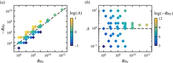
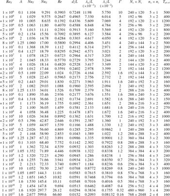
The parameters explored in the present work are shown in figure 1 and more details can be found in Appendix. The numerical method is reported in Ostilla-Mónico et al. (Reference Ostilla-Mónico, Yang, van der Poel, Lohse and Verzicco2015). The typical flow structures are similar to those shown in our previous study (e.g. see figure 1 of Yang et al. (Reference Yang, van der Poel, Ostilla-Mónico, Sun, Verzicco, Grossmann and Lohse2015)). The bulk region is dominated by salt fingers, and thin boundary layers develop for the velocity and salinity fields adjacent to two plates.
Explored parameters shown (a) in the
 $Ra_{S}$
–
 $Ra_{T}$
plane and coloured by
 $\log (\unicode[STIX]{x1D6EC})$
and (b) in the
 $Ra_{S}$
–
 $\unicode[STIX]{x1D6EC}$
plane and coloured by
 $\log (-Ra_{T})$
. The dashed lines indicate
 $\unicode[STIX]{x1D6EC}=1$
, i.e. the fluid layer is neutrally buoyant. The fluid is overall unstable for the parameters below the lines and stable for those above the lines.

3 Global responses and the GL theory
The three key responses of the system are the salinity and heat fluxes and the flow velocity, which are measured in non-dimensional form by the Nusselt and Reynolds numbers as
 $$\begin{eqnarray}\mathit{Nu}_{S}=\frac{\langle u_{3}s\rangle -\unicode[STIX]{x1D705}_{S}\unicode[STIX]{x2202}_{3}\langle s\rangle }{\unicode[STIX]{x1D705}_{S}\unicode[STIX]{x1D6E5}_{S}L^{-1}},\quad \mathit{Nu}_{T}=\frac{\langle u_{3}\unicode[STIX]{x1D703}\rangle -\unicode[STIX]{x1D705}_{T}\unicode[STIX]{x2202}_{3}\langle \unicode[STIX]{x1D703}\rangle }{\unicode[STIX]{x1D705}_{T}\unicode[STIX]{x1D6E5}_{T}L^{-1}},\quad Re=\frac{u_{rms}L}{\unicode[STIX]{x1D708}}.\end{eqnarray}$$
Here
 $\langle \cdot \rangle$
stands for the average over the entire domain and time.
 $u_{rms}$
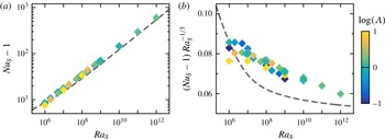
denotes the root-mean-square value of the velocity magnitude. In figure 2 we plot
 $\mathit{Nu}_{S}$
versus
 $\mathit{Ra}_{S}$
, both as a log–log plot and in compensated form. We compare the numerical results to the GL theory with the updated coefficients (Stevens et al.
Reference Stevens, van der Poel, Grossmann and Lohse2013). Note that there is no new free parameter here and the curve is fully determined by the theory. In our previous study (Yang et al.
Reference Yang, van der Poel, Ostilla-Mónico, Sun, Verzicco, Grossmann and Lohse2015) we have shown, for a smaller parameter range, that
 $\mathit{Nu}_{S}$
mainly depends on
 $\mathit{Ra}_{S}$
and it shows only a minor dependence on
 $\unicode[STIX]{x1D6EC}$
. The variation of
 $\mathit{Nu}_{S}$
with
 $\mathit{Ra}_{S}$
is also close to the GL prediction. Indeed, for the current dataset with a much larger parameter range,
 $\mathit{Nu}_{S}$
still follows a single trend which is close to the GL prediction.
Dependences of the convective salinity flux
 $\mathit{Nu}_{S}-1$
on
 $\mathit{Ra}_{S}$
in (a) a log–log plot and (b) compensated form. Symbols are coloured according to the logarithm of
 $\unicode[STIX]{x1D6EC}$
. The dashed lines are the predictions of the GL theory.

Unlike on the salinity flux, however, the density ratio
 $\unicode[STIX]{x1D6EC}$
has strong influence on the flow velocity and on the heat transfer. To reveal the effects of
 $\unicode[STIX]{x1D6EC}$
on the system responses, we focus on two sets of cases with
 $\mathit{Ra}_{S}$
fixed at
 $10^{7}$
and
 $10^{8}$
. Each set consists of six cases with
 $\unicode[STIX]{x1D6EC}$
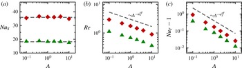
ranging from 0.1 to 10. In figure 3 we plot the dependences of
 $\mathit{Nu}_{S}$
,
 $Re$
and
 $\mathit{Nu}_{T}$
on
 $\unicode[STIX]{x1D6EC}$
for these two sets. Clearly, when
 $\mathit{Ra}_{S}$
is fixed,
 $\mathit{Nu}_{S}$
is almost constant for the range of
 $\unicode[STIX]{x1D6EC}$
considered here. In contrast, for fixed
 $\mathit{Ra}_{S}$
both the Reynolds number
 $Re$
and the convective heat transfer
 $(\mathit{Nu}_{T}-1)$
decrease as
 $\unicode[STIX]{x1D6EC}$
increases from 0.1 to 10. The different behaviours of
 $\mathit{Nu}_{S}$
and
 $Re$
versus
 $\unicode[STIX]{x1D6EC}$
suggest that for fixed salinity difference, increasing the relative strength of the stabilizing temperature difference suppresses the flow velocity. Meanwhile, as will be discussed later in the next section, the horizontal size of the flow structures also changes in a way such that the salinity transfer keeps constant.
Dependences of (a)
 $\mathit{Nu}_{S}$
, (b)
 $Re$
and (c)
 $\mathit{Nu}_{T}-1$
on
 $\unicode[STIX]{x1D6EC}$
for two fixed
 $\mathit{Ra}_{S}=10^{7}$
(green triangles) and
 $10^{8}$
(red diamonds). In (a) the two horizontal dashed lines mark
 $\mathit{Nu}_{S}=18.2$
and 35.9, which are the averaged values over different values of
 $\unicode[STIX]{x1D6EC}$
for each
 $\mathit{Ra}_{S}$
, respectively. In (b) the dashed line indicates the scaling relation
 $\unicode[STIX]{x1D6EC}^{-\unicode[STIX]{x1D6FC}_{u}^{eff}}$
with
 $\unicode[STIX]{x1D6FC}_{u}^{eff}=0.25$
. In (c) the dashed line indicates the scaling relation
 $\unicode[STIX]{x1D6EC}^{-\unicode[STIX]{x1D6FC}_{T}^{eff}}$
with
 $\unicode[STIX]{x1D6FC}_{T}^{eff}=0.75$
.

In figure 3(b) we see the Reynolds number
 $Re$
as function of the density ratio
 $\unicode[STIX]{x1D6EC}$
. Note that even for the larger salinity Rayleigh number
 $\mathit{Ra}_{S}=10^{8}$
and for small
 $\unicode[STIX]{x1D6EC}$
it is never larger than 3, far away from any turbulent behaviour, but reflecting the laminarity of the flow. Also the thermal flux is very small, with
 $\mathit{Nu}_{T}-1$
always being smaller than 1, close to the value for pure molecular diffusion, i.e.
 $\mathit{Nu}_{T}=1$
. From figure 3(b,c) one also observes that the dependences of
 $Re$
and
 $(\mathit{Nu}_{T}-1)$
on
 $\unicode[STIX]{x1D6EC}$
follow certain power-law scalings. Thus a possible strategy for constructing scaling laws for those two quantities would be first extracting the scaling laws of the
 $\unicode[STIX]{x1D6EC}$
dependences of
 $Re$
and
 $(\mathit{Nu}_{T}-1)$
for fixed
 $\mathit{Ra}_{S}$
, and then examining their behaviours for different
 $\mathit{Ra}_{S}$
. This strategy is applied to
 $Re$
and
 $(\mathit{Nu}_{T}-1)$
as follows. Let us assume that
 $Re$
scales as
 $\unicode[STIX]{x1D6EC}^{-\unicode[STIX]{x1D6FC}_{u}^{eff}}$
for fixed
 $\mathit{Ra}_{S}$
, where
 $\unicode[STIX]{x1D6FC}_{u}^{eff}$
is a positive exponent. The minus sign is introduced since
 $Re$
decreases as
 $\unicode[STIX]{x1D6EC}$
increases. The value of
 $\unicode[STIX]{x1D6FC}_{u}^{eff}$
can be determined by the data points in figure 3(b). For the set of
 $\mathit{Ra}_{S}=10^{7}$
, the exponent given by a linear regression is
 $\unicode[STIX]{x1D6FC}_{u}^{eff}=0.24\pm 0.02$
. And for the set of
 $\mathit{Ra}_{S}=10^{8}$
it is
 $\unicode[STIX]{x1D6FC}_{u}^{eff}=0.25\pm 0.02$
. The two values are very close to each other. To obtain a single value for
 $\unicode[STIX]{x1D6FC}_{u}^{eff}$
, we first shift the data points vertically in figure 3(b) such that the two points at
 $(\unicode[STIX]{x1D6EC},\mathit{Ra}_{S})=(1,10^{7})$
and
 $(1,10^{8})$
collapse and then conduct a linear regression with all 12 data points. The final value is
 $\unicode[STIX]{x1D6FC}_{u}^{eff}=0.25\pm 0.02$
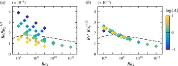
. In figure 4(a) we plot the original values of
 $Re$
compensated by
 $\mathit{Ra}_{S}^{-1/2}$
. The data points are scattered since
 $Re$
is strongly affected by
 $\unicode[STIX]{x1D6EC}$
. However, we can define a rescaled Reynolds number
 $Re^{\ast }=Re\unicode[STIX]{x1D6EC}^{\unicode[STIX]{x1D6FC}_{u}^{eff}}$
with
 $\unicode[STIX]{x1D6FC}_{u}^{eff}=0.25$
. In figure 4(b) we plot
 $Re^{\ast }$
against
 $\mathit{Ra}_{S}$
for the whole dataset. All the data points collapse and the dependence
 $Re^{\ast }(\mathit{Ra}_{S})$
is quite close to the GL prediction. For
 $Re$
we still use the same coefficients as in Stevens et al. (Reference Stevens, van der Poel, Grossmann and Lohse2013) but with a transformation coefficient
 $\unicode[STIX]{x1D6FC}=0.135$
which is determined by the case with
 $\mathit{Ra}_{S}=10^{8}$
and
 $\unicode[STIX]{x1D6EC}=1$
.
(a) Dependence of
 $Re$
versus
 $\mathit{Ra}_{S}$
for all data points. (b) Dependence of the rescaled Reynolds number
 $Re^{\ast }=Re\unicode[STIX]{x1D6EC}^{\unicode[STIX]{x1D6FC}_{u}^{eff}}$
with
 $\unicode[STIX]{x1D6FC}_{u}^{eff}=0.25$
versus
 $\mathit{Ra}_{S}$
for all data points. Symbols are coloured according to the logarithm of
 $\unicode[STIX]{x1D6EC}$
. The dashed lines are the predictions of the GL theory.

In the compensated plots of
 $\mathit{Nu}_{S}$
and
 $Re$
, a discrepancy exits between the numerical results and the GL theory at small
 $\mathit{Ra}_{S}$
. For the RB flows at high Prandtl number, a discrepancy was also found when one applies the GL theory to the RB flows, e.g. see figure 7 of Stevens et al. (Reference Stevens, van der Poel, Grossmann and Lohse2013). Since we directly adopt the original GL theory, it is natural that similar behaviour is observed. Moreover, compared to the RB flow with the same driving Rayleigh number, flow velocity and therefore the Reynolds number are much smaller in the DDC flow due to the extra stabilizing scalar field, especially for small
 $\mathit{Ra}_{S}$
. This may reduce the accuracy of the GL prediction for
 $Re$
at small
 $\mathit{Ra}_{S}$
. Nevertheless, we want to emphasize that the original GL theory already gives predictions with reasonable accuracy.
A similar analysis can be done for
 $\mathit{Nu}_{T}$
. We assume that the convective heat flux scales as
 $(\mathit{Nu}_{T}-1)\sim \unicode[STIX]{x1D6EC}^{-\unicode[STIX]{x1D6FC}_{T}^{eff}}$
and calculate the value of
 $\unicode[STIX]{x1D6FC}_{T}^{eff}$
from figure 3(c) by following the same procedure for
 $\unicode[STIX]{x1D6FC}_{u}^{eff}$
. The final value is
 $\unicode[STIX]{x1D6FC}_{T}^{eff}=0.75\pm 0.03$
. And a rescaled convective heat Nusselt number can be defined as
 $\mathit{Nu}_{T}^{\ast }=(\mathit{Nu}_{T}-1)\unicode[STIX]{x1D6EC}^{\unicode[STIX]{x1D6FC}_{T}^{eff}}$
with
 $\unicode[STIX]{x1D6FC}_{T}^{eff}=0.75$
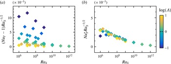
. In figure 5 we plot the original value of
 $\mathit{Nu}_{T}-1$
and the rescaled ones
 $\mathit{Nu}_{T}^{\ast }$
against
 $\mathit{Ra}_{S}$
in a compensated form. Again, the original values are scattered, but the rescaled quantity
 $\mathit{Nu}_{T}^{\ast }$
follows a single trend versus
 $\mathit{Ra}_{S}$
. Two things should be noted from figure 5. First, the quantities are compensated by
 $\mathit{Ra}_{S}^{-1/2}$
as for
 $Re$
, instead of
 $\mathit{Ra}_{S}^{-1/3}$
as for
 $\mathit{Nu}_{S}$
. Second, the dependence of
 $\mathit{Nu}_{T}^{\ast }$
on
 $\mathit{Ra}_{S}$
shown in figure 5(b) is very similar to that of
 $Re^{\ast }$
shown in figure 4(b). A reasonable argument is that in the current flow set-up, the temperature field is stabilizing rather than driving the flow. Thus the convective heat flux is generated as the temperature anomaly is ‘passively’ carried by the flow motions which are sustained by the salinity difference. Therefore
 $\mathit{Nu}_{S}$
behaves similarly to that of a RB flow, while
 $\mathit{Nu}_{T}^{\ast }$
exhibits a similar scaling as
 $Re^{\ast }$
.
(a) Dependence of the convective heat flux
 $\mathit{Nu}_{T}-1$
versus
 $\mathit{Ra}_{S}$
. (b) Dependence of the rescaled heat Nusselt number
 $\mathit{Nu}_{T}^{\ast }=(\mathit{Nu}_{T}-1)\unicode[STIX]{x1D6EC}^{\unicode[STIX]{x1D6FC}_{T}^{eff}}$
with
 $\unicode[STIX]{x1D6FC}_{T}^{eff}=0.75$
versus
 $\mathit{Ra}_{S}$
. Symbols are coloured according to the logarithm of
 $\unicode[STIX]{x1D6EC}$
. Note that the range of the vertical axis in (b) is half of that in (a).

Although the non-dimensional thermal flux is much smaller than the non-dimensional salinity flux, the density-anomaly flux associated with the temperature field may not be negligible when compared to that associated with the salinity field because of the huge difference between the two molecular diffusivities. This can be seen from the density flux ratio which defined as
 $$\begin{eqnarray}R_{f}=\frac{\unicode[STIX]{x1D6FD}_{T}\langle u_{3}\unicode[STIX]{x1D703}\rangle }{\unicode[STIX]{x1D6FD}_{S}\langle u_{3}s\rangle }=\mathit{Le}\unicode[STIX]{x1D6EC}\frac{\mathit{Nu}_{T}-1}{\mathit{Nu}_{S}-1}.\end{eqnarray}$$
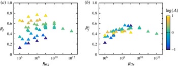
In figure 6(a) we plot the variation of
 $R_{f}$
versus
 $\mathit{Ra}_{S}$
. The density flux ratio
 $R_{f}$
has a value between 0.1 and 0.8. As the density ratio
 $\unicode[STIX]{x1D6EC}$
increases (symbol colour changes from dark blue to light yellow),
 $R_{f}$
also increases. In previous discussion we showed that, for fixed
 $\mathit{Ra}_{S}$
,
 $\mathit{Nu}_{T}-1$
scales as
 $\unicode[STIX]{x1D6EC}^{-\unicode[STIX]{x1D6FC}_{T}^{eff}}$
and
 $\mathit{Nu}_{S}$
is nearly constant. Then by definition (3.2) one expects
 $R_{f}\sim \unicode[STIX]{x1D6EC}^{1-\unicode[STIX]{x1D6FC}_{T}^{eff}}$
for fixed
 $\mathit{Ra}_{S}$
. In figure 6(b) we plot the rescaled density flux ratio
 $R_{f}^{\ast }=R_{f}\unicode[STIX]{x1D6EC}^{\unicode[STIX]{x1D6FC}_{T}^{eff}-1}=R_{f}\unicode[STIX]{x1D6EC}^{-0.25}$
, and indeed all the data points collapse.
(a) Dependence of the density flux ratio
 $R_{f}$
versus
 $\mathit{Ra}_{S}$
. (b) Dependence of the rescaled density flux ratio
 $R_{f}^{\ast }=R_{f}\unicode[STIX]{x1D6EC}^{\unicode[STIX]{x1D6FC}_{T}^{eff}-1}$
with
 $\unicode[STIX]{x1D6FC}_{T}^{eff}=0.75$
versus
 $\mathit{Ra}_{S}$
. Symbols are coloured according to the logarithm of
 $\unicode[STIX]{x1D6EC}$
.

Figure 6(a) indicates that for
 $1<\unicode[STIX]{x1D6EC}\leqslant 10$
,
 $R_{f}$
is between 0.4 and 0.8, which falls into the same range as reported in the previous experiments and simulations, e.g. see Turner (Reference Turner1967), Schmitt (Reference Schmitt1979), McDougall & Taylor (Reference McDougall and Taylor1984), Taylor & Bucens (Reference Taylor and Bucens1989) and Shen (Reference Shen1993). However, in our simulation for fixed
 $\mathit{Ra}_{S}$
, as
 $\unicode[STIX]{x1D6EC}$
increases the density flux ratio
 $R_{f}$
also increases. This is in the opposite trend compared to the results of Shen (Reference Shen1993) where small
 $\unicode[STIX]{x1D6EC}$
generates larger
 $R_{f}$
. The difference is probably caused by the different flow configurations. In our simulations the salt fingers are confined between two boundaries, while in Shen (Reference Shen1993) the finger interfaces grow freely in the vertical direction.
4 Flow structures and thicknesses of boundary layers and fingers
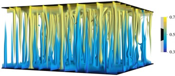
We now turn to the flow structures. We will focus on the horizontal width of the salt fingers and the thicknesses of velocity and salinity boundary layers. Then we will show the horizontal zonal flows which were observed at very high Rayleigh numbers. In all our simulations salt fingers develop in the bulk of the flow domain. A typical flow field can be seen in figure 7, which shows the three-dimensional volume rendering of the salinity field at
 $\mathit{Ra}_{T}=10^{6}$
and
 $\mathit{Ra}_{S}=10^{8}$
(equivalently
 $\unicode[STIX]{x1D6EC}=1$
). The finger layer is bounded by two thin boundary layers adjacent to both plates. The individual salt fingers can be distinguished.
Typical flow structures shown by three-dimensional volume rendering of the salinity field with the flow control parameters
 $\mathit{Ra}_{T}=10^{6}$
and
 $\mathit{Ra}_{S}=10^{8}$
, or equivalently
 $\unicode[STIX]{x1D6EC}=1$
. The colour and opacity are both determined by salinity.

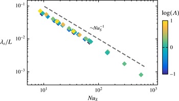
The thickness of the salinity boundary
 $\unicode[STIX]{x1D706}_{s}/L$
versus the salinity Nusselt number
 $\mathit{Nu}_{S}$
. The dashed line has the slope
 $-1$
. Symbols are coloured according to the logarithm of
 $\unicode[STIX]{x1D6EC}$
.

4.1 Salinity boundary layers
The thickness of the salinity boundary layer
 $\unicode[STIX]{x1D706}_{s}$
is defined as the distance from the plate to the location of the first peak of
 $\unicode[STIX]{x1D70E}_{s}(z)$
, which is the standard deviation of salinity over every horizontal plane. In figure 8 we plot the dependence of
 $\unicode[STIX]{x1D706}_{s}/L$
on
 $\mathit{Nu}_{S}$
, and find that it perfectly scales as
 $\mathit{Nu}_{S}^{-1}$
. The scaling
 $\unicode[STIX]{x1D706}_{s}/L\sim \mathit{Nu}_{S}^{-1}$
can be understood by following the argument for RB flows at high Prandtl numbers (Grossmann & Lohse Reference Grossmann and Lohse2001, Reference Grossmann and Lohse2002). The salinity Nusselt number is related to the salinity dissipation rate by the exact relation
 $$\begin{eqnarray}\unicode[STIX]{x1D716}_{s}\equiv \langle \unicode[STIX]{x1D705}_{S}[\unicode[STIX]{x2202}_{i}s]^{2}\rangle =\unicode[STIX]{x1D705}_{S}(\unicode[STIX]{x1D6E5}_{S})^{2}L^{-2}\mathit{Nu}_{S}.\end{eqnarray}$$
For the salinity field with high Prandtl number, the dissipation is dominated by the contribution from the boundary layers. The volume integral of
 $\unicode[STIX]{x1D716}_{s}$
in the two boundary layers may be approximated as
 $$\begin{eqnarray}\unicode[STIX]{x1D716}_{s}\sim \unicode[STIX]{x1D716}_{s}^{\text{BL}}=\langle \unicode[STIX]{x1D705}_{S}[\unicode[STIX]{x2202}_{i}s]^{2}\rangle _{BL}\sim \unicode[STIX]{x1D705}_{S}\left(\frac{\unicode[STIX]{x1D6E5}_{S}}{2\unicode[STIX]{x1D706}_{s}}\right)^{2}\frac{2\unicode[STIX]{x1D706}_{s}}{L}=\unicode[STIX]{x1D705}_{S}\frac{\unicode[STIX]{x1D6E5}_{S}^{2}}{2\unicode[STIX]{x1D706}_{s}L}.\end{eqnarray}$$
Combining the above two equations, one readily obtains
 $\unicode[STIX]{x1D706}_{s}/L\sim \mathit{Nu}_{S}^{-1}$
, which is exactly the case as shown in figure 8.
4.2 The width of the salt fingers
The horizontal length scale of the salt fingers can be determined from the flow field on the horizontal midplane
 $z/L=0.5$
. In figure 9(a,b) we show the contours of the vertical velocity
 $u_{3}$
and the salinity
 $s$
on the horizontal plane
 $z/L=0.5$
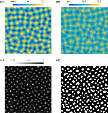
for the same flow field as shown in figure 7. Clearly, most fingers have almost circular shape in the horizontal sections. Some sheet-like links can be found, connecting different fingers, but usually they are not pronounced.
An example of the raw data on the midplane
 $z/L=0.5$
and corresponding finger detection. The control parameters are
 $\mathit{Ra}_{T}=10^{6}$
and
 $\mathit{Ra}_{S}=10^{8}$
, or equivalently
 $\unicode[STIX]{x1D6EC}=1$
. For this flow the standard deviation for the vertical velocity
 $u_{3}$
is
 $\unicode[STIX]{x1D70E}_{u_{3}}=4.9\times 10^{-3}$
and for the salinity
 $s$
is
 $\unicode[STIX]{x1D70E}_{s}=2.9\times 10^{-2}$
. (a,b) Contours of
 $u_{3}$
and
 $s$
, (c) the cross-correlation coefficient between the variances of
 $u_{3}$
and
 $s$
, i.e.
 $(u_{3}^{\prime }s^{\prime })/(\unicode[STIX]{x1D70E}_{u_{3}}\unicode[STIX]{x1D70E}_{s})$
and (d) the finger regions with
 $|s^{\prime }|>\unicode[STIX]{x1D70E}_{s}$
and
 $|u_{3}^{\prime }|>\unicode[STIX]{x1D70E}_{u_{3}}$
, as shown by the white patches.

Large salinity anomaly is usually transported by salt fingers, which can be clearly seen from the cross-correlation between the variance of the vertically velocity
 $u_{3}^{\prime }$
and that of the salinity
 $s^{\prime }$
. The prime denotes the deviation of the quantity from its mean value over the plane. In figure 9(c) we plot the cross-correlation coefficient function
 $C=(u_{3}^{\prime }s^{\prime })/(\unicode[STIX]{x1D70E}_{u_{3}}\unicode[STIX]{x1D70E}_{s})$
with
 $\unicode[STIX]{x1D70E}$
denoting the standard deviation of the quantity.
 $C$
has large negative values at isolated regions, because the ascending (descending) fingers carry negative (positive) salinity anomaly. The global correlation coefficient, which is the average of
 $C$
, is
 $-0.98$
. Thus
 $u_{3}^{\prime }$
and
 $s$
are almost perfectly negatively correlated, namely, salt fingers dominate the salinity transfer in the bulk region. From the flow fields as shown in figure 9(a,b), we can identify the salt-finger regions, which are the regions with
 $|s^{\prime }|>\unicode[STIX]{x1D70E}_{s}$
and
 $|u_{3}^{\prime }|>\unicode[STIX]{x1D70E}_{u_{3}}$
. In figure 9(d) we present the finger regions detected by this method. Each white patch corresponds to an individual finger region. We use two criteria
 $|s^{\prime }|>\unicode[STIX]{x1D70E}_{s}$
and
 $|u_{3}^{\prime }|>\unicode[STIX]{x1D70E}_{u_{3}}$
together instead of only
 $|u_{3}^{\prime }|>\unicode[STIX]{x1D70E}_{u_{3}}$
, so that we can detect individual salt-finger core which has high salinity anomaly and moves in the vertical direction with high velocity.
Such flow fields were stored constantly during each simulation, and the horizontal length scale of the salt finger
 $d$
is extracted from those data. Since the salt fingers become more stable as
 $\unicode[STIX]{x1D6EC}$
increases, the typical time interval between flow fields increases from 5 for small
 $\unicode[STIX]{x1D6EC}$
to 40 for large
 $\unicode[STIX]{x1D6EC}$
. The total number of finger regions
 $N_{f}$
is counted and averaged over time, and the average spatial area occupied by one finger is calculated as
 $A_{f}=A_{total}/N_{f}$
with
 $A_{total}$
being the total horizontal area of the domain. The finger width
 $d$
is then calculated from
 $A_{f}$
by assuming that the finger has circular shape, i.e.
 $d=\sqrt{4A_{f}/\unicode[STIX]{x03C0}}$
. Thus
 $d$
is actually the average diameter of the slender convection cells associated with salt fingers.
Following the argument in Hage & Tilgner (Reference Hage and Tilgner2010), we can relate the scaling behaviour of the finger width to that of the Reynolds number. Since the salinity is mainly transferred by fingers, the salinity Nusselt number can be approximated as
 $$\begin{eqnarray}\mathit{Nu}_{S}\approx \frac{U^{f}\overline{s^{f}}}{\unicode[STIX]{x1D705}_{S}\unicode[STIX]{x1D6E5}_{S}L^{-1}},\end{eqnarray}$$
in which
 $U^{f}$
is the characteristic velocity of the fingers and
 $\overline{s^{f}}$
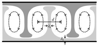
is the mean salinity anomaly within the fingers, respectively. The salinity anomaly is carried from the boundary layers and the side diffusion is weak in the bulk due to the large Prandtl number. Then within each finger convection cell of width
 $d$
, the salinity core has similar width as the thickness of salinity boundary layer, i.e.
 $\unicode[STIX]{x1D706}_{s}$
, as shown by the sketch in figure 10. The mean salinity anomaly inside a finger can then be calculated, for circular fingers, as (Hage & Tilgner Reference Hage and Tilgner2010)
 $$\begin{eqnarray}\overline{s^{f}}=\frac{\unicode[STIX]{x1D6E5}_{S}}{2}\left(\frac{\unicode[STIX]{x1D706}_{s}}{d}\right)^{2}.\end{eqnarray}$$
Then combining the above two equations, and considering that
 $\unicode[STIX]{x1D706}_{s}/L\sim \mathit{Nu}_{S}^{-1}$
as proven in the previous section, one obtains
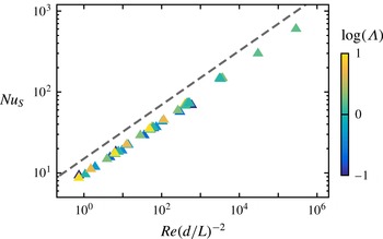
 $$\begin{eqnarray}\frac{U^{f}L}{\unicode[STIX]{x1D705}_{S}}\frac{L^{2}}{d^{2}}\sim \mathit{Nu}_{S}^{3},\quad \text{or}\quad Re\left(\frac{d}{L}\right)^{-2}\sim \mathit{Nu}_{S}^{3}.\end{eqnarray}$$
This scaling relation can be clearly seen in figure 11, in which we plot
 $Re(d/L)^{-2}$
versus
 $\mathit{Nu}_{S}$
for all cases.
A sketch to demonstrate the mean salinity within finger–convection cells.

The scaling between
 $Re(d/L)^{-2}$
and
 $\mathit{Nu}_{S}$
. Symbols are coloured according to the logarithm of
 $\unicode[STIX]{x1D6EC}$
. The dashed line has a slope of
 $1/3$
.

One important consequence of (4.5) is that to generate similar salinity flux
 $\mathit{Nu}_{S}$
, one must have
 $d/L\sim Re^{1/2}$
. For fixed
 $\mathit{Ra}_{S}$
the salinity Nusselt number
 $\mathit{Nu}_{S}$
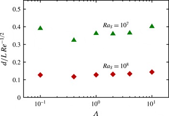
is almost constant. Then the rescaled finger width
 $(d/L)Re^{-1/2}$
should also be constant. In figure 12 we plot the rescaled finger width
 $(d/L)Re^{-1/2}$
for two sets of cases with fixed
 $\mathit{Ra}_{S}=10^{7}$
and
 $10^{8}$
, respectively. Indeed, when
 $\mathit{Ra}_{S}$
is fixed,
 $(d/L)Re^{-1/2}$
is constant for different
 $\unicode[STIX]{x1D6EC}$
, which confirms the scaling
 $d/L\sim Re^{1/2}$
. Furthermore, we have shown in the previous section that
 $Re\sim \unicode[STIX]{x1D6EC}^{-\unicode[STIX]{x1D6FC}_{u}^{eff}}$
with
 $\unicode[STIX]{x1D6FC}_{u}^{eff}=0.25$
for fixed
 $\mathit{Ra}_{S}$
, e.g. see figure 3(b). This implies that
 $d/L\sim \unicode[STIX]{x1D6EC}^{-\unicode[STIX]{x1D6FC}_{u}^{eff}/2}$
for fixed
 $\mathit{Ra}_{S}$
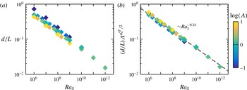
. In figure 13 we show the dependences of both the original finger width
 $d/L$
and the rescaled value
 $(d/L)\unicode[STIX]{x1D6EC}^{\unicode[STIX]{x1D6FC}_{u}^{eff}/2}$
on
 $\mathit{Ra}_{S}$
. The non-dimensional finger width collapses and follows a single power-law scaling when rescaled by
 $\unicode[STIX]{x1D6EC}^{\unicode[STIX]{x1D6FC}_{u}^{eff}/2}$
. A liner regression gives an exponent of
 $-0.24\pm 0.03$
, see figure 13(b).
The dependence of the finger width
 $d/L$
, rescaled as
 $(d/L)Re^{-1/2}$
, on
 $\unicode[STIX]{x1D6EC}$
for two fixed
 $\mathit{Ra}_{S}=10^{7}$
and
 $10^{8}$
.

The dependences of (a) the original finger width
 $d/L$
and (b) the rescaled finger width
 $(d/L)\unicode[STIX]{x1D6EC}^{\unicode[STIX]{x1D6FC}_{u}^{eff}/2}$
with
 $\unicode[STIX]{x1D6FC}_{u}^{eff}=0.25$
on
 $\mathit{Ra}_{S}$
. Symbols are coloured according to the logarithm of
 $\unicode[STIX]{x1D6EC}$
. In (b) the data points collapse after the rescaling, and the dashed line represents the linear regression with a slope of
 $-0.24$
.

4.3 Velocity boundary layers
For the current flow, there is no large-scale circulation in the bulk. The vertically moving fingers induce converging or diverging flows in the horizontal directions when they move away from or towards the plates. Those horizontal motions form the velocity boundary layer. The thickness of velocity boundary layer
 $\unicode[STIX]{x1D706}_{u}$
can be defined as the distance from the boundary to the location of the first peak of
 $\unicode[STIX]{x1D70E}_{u_{h}}(z)$
. Here
 $\unicode[STIX]{x1D70E}_{u_{h}}(z)$
is the standard deviation of one horizontal velocity component over the plane at the height
 $z$
. Since the velocity boundary layer is driven by the vertical motions of the fingers, it is reasonable to expect that
 $\unicode[STIX]{x1D706}_{u}$
scales as the finger width
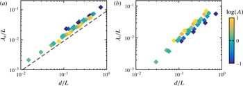
 $d/L$
, which is confirmed by figure 14(a). For comparison, we also plot the salinity boundary layer thickness
 $\unicode[STIX]{x1D706}_{s}/L$
versus
 $d/L$
in figure 14(b). The data points are scattered and no single dependence can be found between
 $\unicode[STIX]{x1D706}_{s}/L$
and
 $d/L$
.
Boundary layer thicknesses of (a) velocity
 $\unicode[STIX]{x1D706}_{u}/L$
and (b) salinity
 $\unicode[STIX]{x1D706}_{s}/L$
versus finger width
 $d/L$
. Symbols are coloured according to the logarithm of
 $\unicode[STIX]{x1D6EC}$
. In (a) the dashed line has a slope unity.

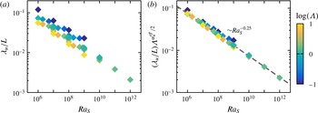
Moreover, figure 15 displays the
 $\mathit{Ra}_{S}$
dependence of
 $\unicode[STIX]{x1D706}_{u}/L$
, which is affected by both
 $\mathit{Ra}_{S}$
and
 $\unicode[STIX]{x1D6EC}$
, as shown in figure 15(a). Similar to the finger width
 $d/L$
, if we rescale
 $\unicode[STIX]{x1D706}_{u}/L$
by
 $\unicode[STIX]{x1D6EC}^{\unicode[STIX]{x1D6FC}_{u}^{eff}/2}$
with
 $\unicode[STIX]{x1D6FC}_{u}^{eff}=0.25$
, all data points collapse onto a single curve, see figure 15(b). The exponent calculated by a linear regression is
 $-0.25\pm 0.02$
, which is very close to the exponent for the rescaled finger width as shown in figure 13(b).
The dependences of (a) the original velocity boundary layer thickness
 $\unicode[STIX]{x1D706}_{u}/L$
and (b) the rescaled velocity boundary layer thickness
 $(\unicode[STIX]{x1D706}_{u}/L)\unicode[STIX]{x1D6EC}^{\unicode[STIX]{x1D6FC}_{u}^{eff}/2}$
with
 $\unicode[STIX]{x1D6FC}_{u}^{eff}=0.25$
on
 $\mathit{Ra}_{S}$
. Symbols are coloured according to the logarithm of
 $\unicode[STIX]{x1D6EC}$
. In (b) the data points collapse after the rescaling, and the dashed line represents the linear regression with a slope of
 $-0.25$
.

4.4 Horizontal zonal flow at high Rayleigh numbers
It is known that large-scale oscillating waves can be excited spontaneously in a fully developed salt-finger field and modulate salt fingers, which is attributed to the collective instability (Stern Reference Stern1969; Holyer Reference Holyer1981; Stern et al.
Reference Stern, Radko and Simeonov2001). These structures, or the internal gravity waves, were observed in simulations of unbounded domains, such as those reported in Stern et al. (Reference Stern, Radko and Simeonov2001) and Stellmach et al. (Reference Stellmach, Traxler, Garaud, Brummell and Radko2011). In the fully periodic domain, the phase planes of gravity waves are not necessarily perpendicular to the gravity direction, and these inclined waves cause strong fluctuations in
 $\mathit{Nu}_{S}$
as they travel in space (Stern et al.
Reference Stern, Radko and Simeonov2001; Stellmach et al.
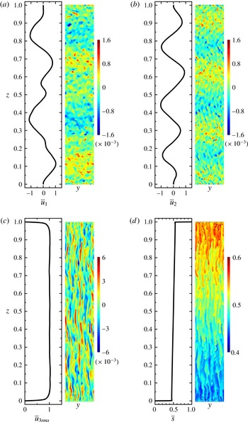
Reference Stellmach, Traxler, Garaud, Brummell and Radko2011). In the current study, the inclined waves did not appear, probably due the vertical constrain of the two plates. Instead, we observed a stack of horizontal zonal flows in alternating directions for the two cases with highest Rayleigh numbers, i.e.
 $\mathit{Ra}_{S}=10^{11}$
and
 $10^{12}$
at a density ratio
 $\unicode[STIX]{x1D6EC}=1.6$
. In figure 16 we show such horizontal zonal flows at
 $\mathit{Ra}_{S}=10^{12}$
, which can be clearly seen from the contours of
 $u_{1}$
and
 $u_{2}$
on the
 $(y,z)$
midplane and the mean profiles in the bulk region, e.g. in the region with
 $0.1<z/L<0.9$
.
The horizontal zonal flow in the case with
 $\mathit{Ra}_{S}=10^{12}$
and
 $\unicode[STIX]{x1D6EC}=1.6$
. The mean profiles (left) and instantaneous contours on the vertical midplane (right) are plotted for the two horizontal velocity components
 $u_{1}$
(a) and
 $u_{2}$
(b), the root-mean-square of the vertical velocity component
 $u_{3rms}$
(c) and the salinity
 $s$
(d). The mean profiles in (a–c) are normalized by the corresponding volume-averaged root-mean-square values
 $\langle u_{1rms}\rangle =3.23\times 10^{-4}$
,
 $\langle u_{2rms}\rangle =3.18\times 10^{-4}$
and
 $\langle u_{3rms}\rangle =1.70\times 10^{-3}$
, respectively.

As
 $\mathit{Ra}_{S}$
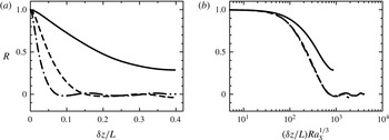
becomes large enough, i.e. for tall samples, individual salt fingers do not extend from one plate to the other. To estimate the vertical length of the salt fingers, the autocorrelation function of the vertical velocity
 $u_{3}$
is calculated in the vertical direction. We use the flow fields on the
 $(y,z)$
midplane as shown in figure 16. Only the data in the range
 $0.1<z/L<0.9$
are used to exclude the boundary layer regions near the two plates. The autocorrelation functions are defined as
 $$\begin{eqnarray}R(\unicode[STIX]{x1D6FF}z)=\frac{\overline{u_{3}(y,z,t)u_{3}(y,z+\unicode[STIX]{x1D6FF}z,t)}}{\overline{u_{3}^{2}(y,z,t)}},\end{eqnarray}$$
where the overline denotes the average over
 $y$
,
 $z$
and
 $t$
on the
 $(y,z)$
midplane. The autocorrelation
 $R$
is computed for three cases with
 $\unicode[STIX]{x1D6EC}=1.6$
and
 $\mathit{Ra}_{S}=10^{10}$
,
 $10^{11}$
and
 $10^{12}$
. The curves are plotted in figure 17(a). For the case with
 $\mathit{Ra}_{S}=10^{10}$
,
 $R$
never decreases to zero, and the fingers can still extend the whole height of the domain. However, for the two cases with larger
 $\mathit{Ra}_{S}$
,
 $R$
does decrease to zero. Thus
 $u_{3}$
decorrelates at a height smaller than the domain height, implying that the average height of the salt fingers is smaller than the domain height
 $L$
. From the curves we determine the first zero point of
 $R$
at
 $\unicode[STIX]{x1D6FF}z/L\approx 0.15$
for
 $\mathit{Ra}_{S}=10^{11}$
and
 ${\approx}0.07$
for
 $\mathit{Ra}_{S}=10^{12}$
. The autocorrelation function
 $R$
is also plotted versus the vertical separation in the viscous scale
 $(\unicode[STIX]{x1D6FF}z/L)\mathit{Ra}_{S}^{1/3}$
, see figure 17(b). Interestingly, the two curves for
 $\mathit{Ra}_{S}=10^{11}$
and
 $10^{12}$
collapse with each other, but they are different from the one for
 $\mathit{Ra}_{S}=10^{10}$
. Note that the three cases have the same density ratio
 $\unicode[STIX]{x1D6EC}=1.6$
. This implies that when the distance between two plates is large enough and fingers cannot extend from one plate to the other, the vertical length of the salt fingers may be set by the density ratio.
The autocorrelation functions of
 $u_{3}$
versus the vertical separations in (a) the global scale
 $\unicode[STIX]{x1D6FF}z/L$
and (b) the viscous scale
 $(\unicode[STIX]{x1D6FF}z/L)\mathit{Ra}_{S}^{1/3}$
, respectively. For all three cases the density ratio is fixed to
 $\unicode[STIX]{x1D6EC}=1.6$
. Solid line:
 $\mathit{Ra}_{S}=10^{10}$
, dashed line:
 $\mathit{Ra}_{S}=10^{11}$
, and dash-dotted line:
 $\mathit{Ra}_{S}=10^{12}$
.

It is interesting to notice that for the case shown in figure 16, the autocorrelation function
 $R$
reaches the first zero point at roughly
 $\unicode[STIX]{x1D6FF}z_{0}/L\approx 0.073$
, e.g. see the dash-dotted curve in figure 17(a). While from figure 16 one observes that the height of the horizontal zonal flow layer is approximately 0.15, close to
 $2\unicode[STIX]{x1D6FF}z_{0}/L$
, which reveals that the length of the salt fingers is the same as the height of the zonal flow layers. Our simulation indicates that although the finger length is smaller than the distance between two plates, they still travel from one plate to the opposite one, i.e. the salinity anomaly is carried by the flow motions between two plates in the form of fingers. There are no large-scale circulations within the zonal flow layers. This is consistent with the observation in the previous section that the appearance of the zonal flow does not change the scaling law of the salinity transfer. Moreover, the horizontal velocity of these zonal flow is quite weak compared to the vertical velocity of salt fingers. Since the height of the zonal flow layers is much larger than the finger width, the horizontal shear introduced by the mean zonal flow is negligible compared to the vertical shear between salt fingers.
We end this subsection by comparing our findings at high Rayleigh numbers to those reported in the literature. In Stellmach et al. (Reference Stellmach, Traxler, Garaud, Brummell and Radko2011), the gravity-wave phase was followed by the spontaneous appearance of a layered phase and staircase-like scalar profiles. Such a transition was not found in our simulation. The reason may be that
 $\mathit{Le}=100$
here is much larger than that in Stellmach et al. (Reference Stellmach, Traxler, Garaud, Brummell and Radko2011). In our case the layered phase may occur at higher
 $\mathit{Ra}_{S}$
. More simulations are needed to clarify whether and when the layered phase can be realised in the current configuration. In the experiments of a salt–sugar system wavy fingers were also observed both in the single finger layer occupying the entire tank or even in the finger layers bounded by two convection layers as in the staircase state (Krishnamurti Reference Krishnamurti2003). However, they did not appear in the experiments of Hage & Tilgner (Reference Hage and Tilgner2010) and Kellner & Tilgner (Reference Kellner and Tilgner2014). The exact conditions for the appearance of zonal flows and wavy fingers are not clear at this stage. The present Lewis number
 $\mathit{Le}=100$
is smaller than those in Tilgner’s experiments (
 $\mathit{Le}\approx 240$
) but larger than those in Krishnamurti (Reference Krishnamurti2003) (
 $\mathit{Le}\approx 3$
), while the
 $\mathit{Ra}_{S}$
for obtaining wavy fingers in our simulations is comparable to the highest
 $\mathit{Ra}_{S}$
in Tilgner’s experiments and much smaller than the
 $\mathit{Ra}_{S}$
across the whole tank in Krishnamurti (Reference Krishnamurti2003).
5 Scaling laws for Hage & Tilgner’s experiments
For the scaling laws proposed in the previous two sections, one has to fit two exponents from the numerical results to collapse the data, i.e.
 $\unicode[STIX]{x1D6FC}_{u}^{eff}$
for the Reynolds number
 $Re$
and
 $\unicode[STIX]{x1D6FC}_{T}^{eff}$
for the convective heat flux
 $\mathit{Nu}_{T}-1$
. The scaling laws for the flow structures, such as the finger width and the thickness of velocity boundary layers, can be deduced from the scaling of
 $Re$
. In our simulations only one combination of Prandtl number
 $(\mathit{Pr}_{T},\mathit{Pr}_{S})=(7,700)$
is considered. One may expect that the values of these exponents depend on the Prandtl number and should vary for different fluid system.
In order to test the scaling laws for the different fluid systems, we perform the previous analysis on the experimental data of Hage & Tilgner (Reference Hage and Tilgner2010) which have
 $(\mathit{Pr}_{T},\mathit{Pr}_{S})\approx (9,2200)$
. Our previous study revealed that the GL prediction for the salinity transfer agrees with the experimental results (Yang et al.
Reference Yang, van der Poel, Ostilla-Mónico, Sun, Verzicco, Grossmann and Lohse2015). Here we further show that a complete description of the experimental results can be obtained by following the method described in the previous sections. In the experiments the heat flux was not measured, and we focus on the Reynolds number and the finger width. Recent studies revealed that when the density ratio is very small, the salt fingers will be replaced by large-scale convection rolls and the flow becomes very similar to the RB case (Kellner & Tilgner Reference Kellner and Tilgner2014; Yang, Verzicco & Lohse Reference Yang, Verzicco and Lohse2016a
). To confine ourselves to the salt-finger regime and be consistent with the current parameter range, we discard the data points with
 $\unicode[STIX]{x1D6EC}<0.1$
in the dataset of Hage & Tilgner (Reference Hage and Tilgner2010).
To obtain the scaling laws for
 $Re$
and
 $d/L$
, the only exponent we need to fit is
 $\unicode[STIX]{x1D6FC}_{u}^{eff}$
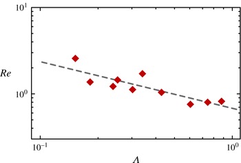
. Since in the experiment it is very difficult to set the control parameters precisely, we choose ten cases within a narrow range
 $10^{9}<\mathit{Ra}_{S}<2\times 10^{9}$
, see figure 18. By a linear regression we obtain
 $Re\sim \unicode[STIX]{x1D6EC}^{-\unicode[STIX]{x1D6FC}_{u}^{eff}}$
with
 $\unicode[STIX]{x1D6FC}_{u}^{eff}=0.54\pm 0.10$
. Similarly, we define the rescaled Reynolds number as
 $Re^{\ast }=Re\unicode[STIX]{x1D6EC}^{\unicode[STIX]{x1D6FC}_{u}^{eff}}$
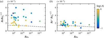
. In figure 19 we plot both
 $Re$
and
 $Re^{\ast }$
against
 $\mathit{Ra}_{S}$
for the experimental results with
 $\unicode[STIX]{x1D6EC}\geqslant 0.1$
in a compensated form, and compare the results with the GL theory. Here for the model coefficients we use the same values as given in Stevens et al. (Reference Stevens, van der Poel, Grossmann and Lohse2013), and a transformation coefficient
 $\unicode[STIX]{x1D6FC}=0.027$
. Indeed, compared to the original values the rescaled Reynolds number
 $Re^{\ast }$
collapses and is very close to the GL prediction.
Dependences of
 $Re$
on
 $\unicode[STIX]{x1D6EC}$
for the experimental data from Hage & Tilgner (Reference Hage and Tilgner2010) with
 $\mathit{Ra}_{S}\in (10^{9},2\times 10^{9})$
and
 $\unicode[STIX]{x1D6EC}\geqslant 0.1$
. The dashed line indicates the linear regression giving
 $Re\sim \unicode[STIX]{x1D6EC}^{-\unicode[STIX]{x1D6FC}_{u}^{eff}}$
with
 $\unicode[STIX]{x1D6FC}_{u}^{eff}=0.54$
.

(a) Dependence of
 $Re$
versus
 $\mathit{Ra}_{S}$
for the experimental data from Hage & Tilgner (Reference Hage and Tilgner2010) with
 $\unicode[STIX]{x1D6EC}\geqslant 0.1$
. (b) The same data of (a) but rescaled as
 $Re^{\ast }=Re\unicode[STIX]{x1D6EC}^{\unicode[STIX]{x1D6FC}_{u}^{eff}}$
with
 $\unicode[STIX]{x1D6FC}_{u}^{eff}=0.54$
. Symbols are coloured according to the logarithm of
 $\unicode[STIX]{x1D6EC}$
. The dashed lines are the predictions of the GL theory.

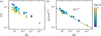
A rescaled finger width can be defined accordingly as
 $(d/L)\unicode[STIX]{x1D6EC}^{\unicode[STIX]{x1D6FC}_{u}^{eff}/2}$
with
 $\unicode[STIX]{x1D6FC}_{u}^{eff}=0.54$
. In figure 20 we plot the original and rescaled values of the finger width. The rescaled values collapse and its dependence on
 $\mathit{Ra}_{S}$
follows a power-law scaling. The exponent obtained by a linear regression is
 $-0.23\pm 0.04$
. This value is very similar to that for
 $(\mathit{Pr}_{T},\mathit{Pr}_{S})=(7,700)$
, i.e.
 $-0.24\pm 0.03$
as given in § 4.2. However, based on the current results it is not clear whether this exponent is universal for different Prandtl numbers.
(a) The original finger width
 $d/L$
and (b) the rescaled finger width
 $(d/L)\unicode[STIX]{x1D6EC}^{\unicode[STIX]{x1D6FC}_{u}^{eff}/2}$
with
 $\unicode[STIX]{x1D6FC}_{u}^{eff}=0.54$
for the experimental data from Hage & Tilgner (Reference Hage and Tilgner2010) with
 $\unicode[STIX]{x1D6EC}\geqslant 0.1$
. Symbols are coloured according to the logarithm of
 $\unicode[STIX]{x1D6EC}$
. In (b) the data points collapse after the rescaling and the dashed line represents the linear regression with slope
 $-0.23$
.

It should be pointed out that our scaling relations are very close to those given in Hage & Tilgner (Reference Hage and Tilgner2010). Hage & Tilgner (Reference Hage and Tilgner2010) proposed
 $Re\sim \mathit{Ra}_{T}^{-1/2}\mathit{Ra}_{S}\sim \unicode[STIX]{x1D6EC}^{-1/2}\mathit{Ra}_{S}^{1/2}$
. From figure 19(b) one observes that
 $Re^{\ast }\mathit{Ra}_{S}^{-1/2}$
decreases very slowly as
 $\mathit{Ra}_{S}$
increases. In other words, the current scaling law for the Reynolds number is approximately
 $Re\sim \unicode[STIX]{x1D6EC}^{-0.54}\mathit{Ra}_{S}^{0.5}$
. For the finger width, Hage & Tilgner (Reference Hage and Tilgner2010) determined
 $d/L\sim \mathit{Ra}_{T}^{-1/3}\mathit{Ra}_{S}^{1/9}\sim \unicode[STIX]{x1D6EC}^{-1/3}\mathit{Ra}_{S}^{-2/9}$
, while our analysis gives
 $d/L\sim \unicode[STIX]{x1D6EC}^{-0.27}\mathit{Ra}_{S}^{-0.23}$
. Furthermore, Hage & Tilgner (Reference Hage and Tilgner2010) suggested that
 $\mathit{Nu}_{S}\sim \mathit{Ra}_{T}^{-1/12}\mathit{Ra}_{S}^{4/9}\sim \unicode[STIX]{x1D6EC}^{-1/12}\mathit{Ra}_{S}^{13/36}$
, i.e. a very weak dependence on
 $\unicode[STIX]{x1D6EC}$
and for
 $\mathit{Ra}_{S}$
an exponent very close to
 $1/3$
.
Finally, we want to stress that the effective exponents
 $\unicode[STIX]{x1D6FC}_{u}^{eff}$
and
 $\unicode[STIX]{x1D6FC}_{T}^{eff}$
take different values for different fluid system, i.e. they depend on two Prandtl numbers. In table 1 we summarise the values of
 $\unicode[STIX]{x1D6FC}_{u}^{eff}$
and
 $\unicode[STIX]{x1D6FC}_{T}^{eff}$
for three different combinations of
 $\mathit{Pr}_{T}$
and
 $\mathit{Pr}_{S}$
, i.e. the current data, the experimental data from Hage & Tilgner (Reference Hage and Tilgner2010) and one group of data from Yang et al. (Reference Yang, Verzicco and Lohse2016a
) with
 $(\mathit{Pr}_{T},\mathit{Pr}_{S})=(7,70)$
,
 $\mathit{Ra}_{S}=10^{8}$
and
 $0.1\leqslant \unicode[STIX]{x1D6EC}\leqslant 1.0$
. For the last dataset, the finger regime occupies a smaller range of
 $\unicode[STIX]{x1D6EC}$
because
 $\mathit{Le}$
is smaller compared to the other two datasets. More simulations are needed, especially at different Prandtl numbers, to fully understand the physical origin of these exponents.
The effective exponents
 $\unicode[STIX]{x1D6FC}_{u}^{eff}$
and
 $\unicode[STIX]{x1D6FC}_{T}^{eff}$
for different combinations of
 $\mathit{Pr}_{T}$
and
 $\mathit{Pr}_{S}$
.

6 Conclusions
A systematic numerical study is carried out for DDC flow bounded by two parallel plates at Prandtl numbers of
 $\mathit{Pr}_{T}=7$
and
 $\mathit{Pr}_{S}=700$
, which are similar to the values for seawater. The salinity Rayleigh number
 $\mathit{Ra}_{S}$
covers six decades in order of magnitude, i.e. from
 $10^{6}$
to
 $10^{12}$
, and the density ratio
 $\unicode[STIX]{x1D6EC}$
is between 0.1 to 10. The salinity Nusselt number
 $\mathit{Nu}_{S}$
depends mainly on
 $\mathit{Ra}_{S}$
. The dependence of
 $\mathit{Nu}_{S}$
on
 $\mathit{Ra}_{S}$
is well captured by the GL theory with the same coefficients as determined for RB flow. For fixed
 $\mathit{Ra}_{S}$
, as the density ratio
 $\unicode[STIX]{x1D6EC}$
increases,
 $\mathit{Nu}_{S}$
is constant, while both the Reynolds number
 $Re$
and the convective heat flux
 $\mathit{Nu}_{T}-1$
decrease according to certain power-law scalings, namely
 $Re\sim \unicode[STIX]{x1D6EC}^{-\unicode[STIX]{x1D6FC}_{u}^{eff}}$
and
 $(\mathit{Nu}_{T}-1)\sim \unicode[STIX]{x1D6EC}^{-\unicode[STIX]{x1D6FC}_{T}^{eff}}$
. The two exponents are calculated from the numerical results, and for
 $(\mathit{Pr}_{T},\mathit{Pr}_{S})=(7,700)$
the values are
 $\unicode[STIX]{x1D6FC}_{u}^{eff}=0.25\pm 0.02$
and
 $\unicode[STIX]{x1D6FC}_{T}^{eff}=0.75\pm 0.03$
. Then the rescaled Reynolds number and convective heat flux are introduced as
 $Re^{\ast }=Re\unicode[STIX]{x1D6EC}^{\unicode[STIX]{x1D6FC}_{u}^{eff}}$
and
 $\mathit{Nu}_{T}^{\ast }=(\mathit{Nu}_{T}-1)\unicode[STIX]{x1D6EC}^{\unicode[STIX]{x1D6FC}_{T}^{eff}}$
. After rescaling, both
 $Re^{\ast }$
and
 $\mathit{Nu}_{T}^{\ast }$
collapse for different
 $\unicode[STIX]{x1D6EC}$
and exhibit similar dependences on
 $\mathit{Ra}_{S}$
. We have interpreted this finding as the (stabilising) temperature field being advected by the velocity field like a passive scalar.
For fixed
 $\mathit{Ra}_{S}$
and varying
 $\unicode[STIX]{x1D6EC}$
, salt fingers have different horizontal size and velocity but transfer salinity with a similar rate. The flow fields on the horizontal midplane indicate that salt fingers usually are circular in the horizontal sections. To generate a similar salinity flux at different density ratio, the horizontal width of salt fingers must scale as
 $d/L\sim Re^{1/2}\sim \unicode[STIX]{x1D6EC}^{-0.125}$
for fixed
 $\mathit{Ra}_{S}$
. Our numerical results confirm this argument, and the rescaled finger width
 $(d/L)\unicode[STIX]{x1D6EC}^{0.125}$
follows a single power-law scaling versus
 $\mathit{Ra}_{S}$
. In the current flow, the velocity boundary layer is driven by the vertical motion of salt fingers, and its thickness follows the same scaling laws as the finger width. The thickness of the salinity boundary layer, however, scales perfectly as
 $\unicode[STIX]{x1D706}_{s}/L\sim \mathit{Nu}^{-1}$
, which is a natural result from the global balance between the salinity dissipation and Nusselt number, and the fact that the total salinity dissipation is dominated by the contribution from the boundary layers.
The scaling laws proposed for our numerical results are also tested against the experimental data of Hage & Tilgner (Reference Hage and Tilgner2010) with
 $(\mathit{Pr}_{T},\mathit{Pr}_{S})\approx (9,2200)$
. The exponent
 $\unicode[STIX]{x1D6FC}_{u}^{eff}$
now has the value
 $0.54\pm 0.10$
. The rescaling of the Reynolds number and the finger width with this new
 $\unicode[STIX]{x1D6FC}_{u}^{eff}$
collapses the data points for all experimental cases with
 $\unicode[STIX]{x1D6EC}\geqslant 0.1$
. The dependence of the rescaled Reynolds number on
 $\mathit{Ra}_{S}$
is very close to the GL prediction. The two effective exponents
 $\unicode[STIX]{x1D6FC}_{u}^{eff}$
and
 $\unicode[STIX]{x1D6FC}_{T}^{eff}$
are also calculated for an additional set of numerical results with
 $(\mathit{Pr}_{T},\mathit{Pr}_{S})=(7,70)$
,
 $\mathit{Ra}_{S}=10^{8}$
and
 $0.1\leqslant \unicode[STIX]{x1D6EC}\leqslant 1.0$
. Their values are
 $\unicode[STIX]{x1D6FC}_{u}^{eff}=0.66\pm 0.08$
and
 $\unicode[STIX]{x1D6FC}_{T}^{eff}=0.54\pm 0.03$
, respectively. All these different values of
 $\unicode[STIX]{x1D6FC}_{u}^{eff}$
and
 $\unicode[STIX]{x1D6FC}_{T}^{eff}$
for different
 $(\mathit{Pr}_{T},\mathit{Pr}_{S})$
indicate that the two exponents depend on the properties of the fluid system, and more simulations are needed to fully understand their physical origins.
When
 $\mathit{Ra}_{S}$
is high enough, a stack of horizontal zonal flows emerge in the bulk region and have alternative flow directions. For the fluid system considered here, these zonal flow appears when
 $\mathit{Ra}_{S}\geqslant 10^{11}$
. For these large
 $\mathit{Ra}_{S}$
– corresponding to a large separation between the two plates – the salt fingers cannot extend from one plate to the opposite one, but instead have a vertical length which is smaller than the domain height. The inclined gravity waves, which were reported for the fully periodic simulations, were not observed in our bounded flows. This is probably due to the vertical constraint of the plates.
The current results propose various problems for future studies. The present scaling strategy should be further validated with other combinations of Prandtl numbers. Since the Prandtl numbers in our simulations are similar to those of seawater, it is of great interests to test the applicability of the current scaling relations to oceanic salt-finger layers. The first step would be the comparison between the current results and DDC flows bounded by two free-slip plates. The latter step-up is more similar to the oceanic salt-finger layers. Such a study has been carried out and is reported in another paper (Yang, Verzicco & Lohse Reference Yang, Verzicco and Lohse2016b
). The same methodology may also be used to develop scaling relations for DDC in the diffusive regime, where the flow is driven by an unstable temperature difference and stabilized by a salinity difference. Finally, in our simulations, even at
 $\mathit{Ra}_{S}=10^{12}$
, we did not observe the staircase state with alternating finger and convection layers. Determining the control parameters at which the staircase state will be realised in the current flow configuration would be very interesting and highly desired but requires more simulations.
Acknowledgements
This study is supported by Foundation for Fundamental Research on Matter, and by the Netherlands Center for Multiscale Catalytic Energy Conversion (MCEC), an NWO Gravitation programme funded by the Ministry of Education, Culture and Science of the government of the Netherlands. The computing resources were provided by the Dutch national e-infrastructure of SURFsara, and the Italian supercomputer FERMI at CINECA under PRACE project no. 2015133124.
Appendix. Numerical details
In table 2 we provide the details of our numerical simulations.
Summary of the control parameters and the numerical results. For all simulations
 $\mathit{Pr}_{T}=7$
and
 $\mathit{Pr}_{S}=700$
. Columns from left to right: the salinity Rayleigh numbers
 $\mathit{Ra}_{S}$
, the density ratio
 $\unicode[STIX]{x1D6EC}$
, the heat and salinity Nusselt numbers
 $\mathit{Nu}_{T}$
and
 $\mathit{Nu}_{S}$
, the Reynolds number
 $Re$
, the finger width
 $d/L$
, the thicknesses of velocity and salinity boundary layers
 $\unicode[STIX]{x1D706}_{u}$
and
 $\unicode[STIX]{x1D706}_{s}$
, the aspect ratio
 $\unicode[STIX]{x1D6E4}$
of the computational domain, the base resolutions and refinement factors in the
 $x$
and
 $z$
directions, respectively. The domain size and resolution in the
 $y$
direction are the same as those in the
 $x$
direction. Asterisks mark the cases from Yang et al. (Reference Yang, van der Poel, Ostilla-Mónico, Sun, Verzicco, Grossmann and Lohse2015), in which the Reynolds number was consistently underestimated by approximately 20 % due to a round-off error introduced in the original post processing analysis. Here all these values were corrected.