1. Introduction
Many unexpected phenomena have been discovered when a channel size is reduced to the angstrom scale, where flow and transport behaviours are not capable of being understood by classical electrical double layer theories (Bocquet & Charlaix Reference Bocquet and Charlaix2010; Kavokine, Netz & Bocquet Reference Kavokine, Netz and Bocquet2021; Monet, Bocquet & Bocquet Reference Monet, Bocquet and Bocquet2023; Xu, Yan & Xie Reference Xu, Yan and Xie2024; Zhang, Fu & Xie Reference Zhang, Fu and Xie2024). At such small scales, many anomalous behaviours of fluids and ions differ from existing knowledge, such as anomalous dielectric constants (Huang et al. Reference Huang, Cottin-Bizonne, Ybert and Bocquet2007,Reference Huang, Cottin-Bizonne, Ybert and Bocquet2008; Fumagalli et al. Reference Fumagalli2018), fast water transport (Holt et al. Reference Holt, Park, Wang, Stadermann, Artyukhin, Grigoropoulos, Noy and Bakajin2006; Secchi et al. Reference Secchi, Marbach, Niguès, Stein, Siria and Bocquet2016; Emmerich et al. Reference Emmerich, Vasu, Niguès, Keerthi, Radha, Siria and Bocquet2022; Itoh et al. Reference Itoh2022), fractional Wien effects (Kavokine et al. Reference Kavokine, Marbach, Siria and Bocquet2019) and the breakdown of the Nernst–Einstein relation (Li et al. Reference Li, Misra, Li, Yao, Zhao, Zhang, Chen, Blankschtein and Noy2023). The friction (Fu, Merabia & Joly Reference Fu, Merabia and Joly2017; Xie et al. Reference Xie, Fu, Niehaus and Joly2020), confinement (Fu, Merabia & Joly Reference Fu, Merabia and Joly2018; Zhou & Xu Reference Zhou and Xu2020) and dehydration (Yu et al. Reference Yu, Fan, Xia, Zhu, Wu and Wang2019) effects all have significant impacts on the behaviour of ions.
While much current research has focused on ionic transport under an applied electric field, less attention has been given to streaming currents driven by applied pressure in angstrom channels. This discrepancy may arise from the fact that the experiments have predominantly been conducted using two-dimensional materials, which are typically non-charged. A few approaches, such as successfully polarising two-dimensional materials by voltage gating (Mouterde et al. Reference Mouterde, Keerthi, Poggioli, Dar, Siria, Geim, Bocquet and Radha2019) and plasma activation (Emmerich et al. Reference Emmerich, Vasu, Niguès, Keerthi, Radha, Siria and Bocquet2022), have revealed new electrokinetic phenomena in angstrom channels. Mouterde et al. (Reference Mouterde, Keerthi, Poggioli, Dar, Siria, Geim, Bocquet and Radha2019) discovered that the magnitude of the streaming current could be enhanced up to 20 times via voltage gating in angstrom channels. In addition, the streaming current increases linearly with the pressure gradient in raw carbon nanotubes but may exhibit a complex coupling with the applied voltage. Under voltage gating conditions, the streaming current shows a parabolic increase with applied pressure, as reported by Marcotte et al. (Reference Marcotte, Mouterde, Niguès, Siria and Bocquet2020). To our knowledge, this is the only experimental evidence of nonlinear streaming current in angstrom channels so far. Other findings, including molecular dynamics (MD) simulation (Monet et al. Reference Monet, Bocquet and Bocquet2023), reported a linear relationship between streaming currents and applied pressure even in the absence of surface charges, which is possibly due to the selectivity of ions in porous nanostructures, possibly different from our mechanisms.
Due to the anomalous dielectric constant of water in angstrom channels (Fumagalli et al. Reference Fumagalli2018), the self-energy of a single ion and ion–ion interactions in confinement are strongly reinforced (Zhou & Xu Reference Zhou and Xu2020; Kavokine, Robin & Bocquet Reference Kavokine, Robin and Bocquet2022). The electrical double layer concept may fail to describe the ionic distribution and ion–wall interactions at the angstrom scale, resulting in unclear electrokinetic phenomena. In particular, the charge distribution on the surface may significantly influence the slip length and zeta potential (Xie et al. Reference Xie, Fu, Niehaus and Joly2020), which originate from the dissociation process or physical adsorption at the dielectric interfaces (Behrens & Grier Reference Behrens and Grier2001; Stein, Kruithof & Dekker Reference Stein, Kruithof and Dekker2004; Xie et al. Reference Xie, Shi, Wang and Wang2023), as well as from a homogeneously charged surface at metal-like surfaces. Our previous experimental results (Xie et al. Reference Xie, Shi, Wang and Wang2023) demonstrated that ionic conduction under bias voltage exhibits a strong nonlinear feature for the I–V curve of latent-track angstrom channels, likely due to the counterion blockade at carboxyl groups on the channel walls. Such nonlinear I–V curves were explained by MD simulations and one-dimensional non-equilibrium statistical mechanics in heterogeneously charged angstrom channels (Zhang et al. Reference Zhang, Fu and Xie2024). Recent experimental evidence further shows that streaming conductance becomes pressure-dependent in latent-track angstrom channels with deprotonated carboxyl groups on the surface, a phenomenon that may be absent in nanofluidic channels with radii exceeding a few nanometres (Lu et al. Reference Lu, Luan, Guo, Duan, Du and Xie2024).
In this work, we investigate the flow of water molecules and ionic transport in a charged angstrom nanotube, considering both homogeneously and heterogeneously charged surfaces as toy models. In the homogeneously charged system, where all atoms on the wall carry identical fractional charges to model a metal-like carbon nanotube (CNT) or graphene, we find that both water flow velocity and the streaming current increase linearly with the pressure gradient, consistent with classical electrokinetic theories. In the heterogeneously charged system, we randomly place a charged atom (
 $-e$
) along the circumference of the nanotube with a periodic interval of 25 Å in the axial direction, representing deprotonated/dissociated groups on the wall. In a high-friction wall system, where liquid–wall friction dominates, we find the water flow velocity increases linearly with the pressure gradient, while the streaming current increases nonlinearly. In a low-frictional wall system, our simulation results show that both streaming current and water flow velocity exhibit strong nonlinear increases with the pressure gradient, resulting in a pressure-dependent streaming conductance. We further investigated voltage-driven ionic transport and electro-osmosis in confinement. Simulation results revealed a linear response in homogeneously charged systems but a nonlinear behaviour in heterogeneously charged systems.
To quantify this process, we employ one-dimensional non-equilibrium statistics using the Fokker–Planck equation to estimate the first mean passage time of counterions due to the Coulomb interactions of surface charge for the high-friction limit and low-friction limit of a nanotube wall. Additionally, we apply a Markov chain stochastic model to describe the sequence evolution in the low-friction system, where water flow and ionic transport are highly coupled. We find a threshold applied pressure for an observable streaming current (∼
 $1e/10\,\rm ns$
), at which counterions dissociate from the surface charge, generating a current within the time scale of the MD simulation. Such critical pressure may gradually decrease as the channel radius increases, as the enhanced dielectric constant of confined water weakens Coulomb interactions between counterions and surface charges (Fumagalli et al. Reference Fumagalli2018). We derive formulas for the streaming current, permeability and surface potential in a charged angstrom channel, which may be helpful for understanding electrokinetic transport phenomena in charged angstrom channels and for potential applications like ion separations.
2. System and methods
2.1. Homogeneously charged system
(a) Schematic of the homogeneously charged system, where each wall atom carries a charge of
 $-20e/N_c$
with
 $N_c$
being the number of atoms on the nanotube wall. The green line schematically represents a smooth free energy drop of a free cation under pressure-driven flow. (b) Schematic of a heterogeneously charged system, where a wall atom (green) is periodically charged with
 $-e$
at intervals of 25 Å. The green line illustrates the potential well due to Coulomb interaction between cation and surface charge under hydrodynamic friction.

We first constructed a zigzag CNT water channel using the LAMMPS software package for full atomic MD simulations (Thompson et al. Reference Thompson2022), with radii
 $R$
from 5.48 to 7.05 Å and a length
 $L$
of 501.97 Å. Interactions between atoms were described using the Lennard-Jones (LJ) 12-6 potential:
 $\phi (r)=4\epsilon _{ij} [({\sigma _{ij}}/{r})^{12}-({\sigma _{ij}}/{r})^6]$
.
Taking a CNT with a radius of
 $5.48$
Å as an example, each atom at the nanotube wall is charged with a density of
 $\varSigma = -20e/N_c$
, where
 $\varSigma$
and
 $N_c$
denote the surface charge density and the number of atoms on the wall, respectively. The homogeneously charged system represents a metal-like surface (CNT or graphene) as shown in figure 1(a). Twenty sodium ions were placed inside the nanotube, consistent with the heterogeneously charged system discussed later.
2.2. Heterogeneously charged system
For the heterogeneously charged wall system, 20 negatively charged carbon atoms (
 $-e$
) were periodically placed at 25 Å intervals, randomly distributed along the circumference of the CNT cross-sections, as shown in figure 1(b). For comparison, the surface charge density was kept the same as that for the homogeneously charged surface. All counterions were bound to the surface charge after thermal relaxation, which was performed at a temperature of 298 K.
We employed the TIP3P water molecules (Jorgensen et al. Reference Jorgensen, Chandrasekhar, Madura, Impey and Klein1983), and the ion (
 $\rm Na^+$
,
 $\rm K^+$
,
 $\rm Li^+$
and
 $\rm Cl^-$
) model by Joung & Cheatham (Reference Joung and Cheatham2008), using a scaling charge factor of 0.85 (Biriukov, Kroutil & Předota Reference Biriukov, Kroutil and Předota2018). The water–carbon interactions were based on previous studies (Werder et al. Reference Werder, Walther, Jaffe, Halicioglu and Koumoutsakos2003) and simulations were conducted at 298 K using Nosé–Hoover thermostats in the
 $x$
and
 $y$
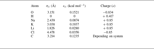
directions. Heteronuclear LJ parameters were calculated using the Lorentz–Berthelot mixing rules, with detailed parameters listed in table 1.
The LJ force fields and charges of homonuclear atoms. Heteronuclear LJ parameters are computed with Lorentz–Berthelot mixing rules.

In all simulations, the CNTs and water molecules were kept as rigid structures, and carbon atoms in the CNT were fixed with a C–C bond length of 1.42 Å. The cutoff radius for LJ and Coulomb interactions was set to 10 Å, with a time step of 1
 $\rm fs$
. The calculation of long-range Coulomb interactions utilised the particle–particle particle–mesh algorithm, and periodic boundary conditions were applied in all directions. We simulated the phenomena induced by applying pressures to the molecules in the system and statistically counted the fluxes of ions caused by the hydrodynamic friction of water molecules. Each simulation was run for a duration of 40 ns to ensure that the system reached an equilibrium state, with data from the first 3 ns excluded to avoid memory effects.
3. Results and discussion
We investigated the streaming current in the nanotube systems with homogeneously and heterogeneously charged systems. Twenty
 $\rm Na^+$
ions were placed inside the nanotube for a neutral system. In the heterogeneously charged channel, the
 $\rm Na^+$
ions were initially adsorbed at the negatively charged sites on the wall after thermal relaxation. In contrast, in the homogeneously charged channel, the
 $\rm Na^+$
ions were freely distributed within the nanotube. We applied a volume force
 $ f_i$
to all atoms in the electrolyte solution to simulate an externally applied pressure. The pressure gradient was calculated using the formula
 $ -\nabla P = f_V = f_i N_0/V$
, where
 $ N_0$
is the number of particles in the electrolyte solution and
 $ V$
is the volume of the nanotube. The simulations were performed to obtain values for ion fluxes and water velocity, and we used the equation
 $I = ({e}/{L}) {\sum}_{i=1}^{N} v_i$
to calculate the total streaming current of the system, where
 $N$
is the number of ions and
 $v_i$
is the average velocity of the
 $i$
th ion in the
 $z$
direction. All statistical results are averaged over six independent MD simulations, with each initialised with a different random velocity distribution of atoms. Error bars represent the range across these six simulations.
3.1. Homogeneously charged nanotube
(a) The trajectory of three identical
 $\rm Na^+$
cations (red) and a water molecule (blue) under a pressure gradient of 0.93 bar Å−1 moving with an identical velocity in the homogeneously charged system. (b) The streaming current and (c) water fluxes in the homogeneously charged system (red) and heterogeneously system (blue). The symbols are derived from simulation, while the solid lines denote the theoretical results for ions by (4.5) and water flow rate
 $Q=\pi R^2v_w$
by (4.4).

In homogeneously charged systems, our results show that the streaming current as well as the water flow flux increase linearly with the applied pressure (see yellow dots and dashed lines in figure 2 b,c), which can be understood by the classical electrokinetic theories using a proper surface potential. At equilibrium state, all ions and water molecules have nearly the same constant velocities, as seen in figure 2(a), where the trajectories of three selected counterions are recorded as coordinates change over the time of simulation. The results also indicate that there is no relative motion between counterions and water molecules. In contrast, no observable counterion dissociation occurs within the time of MD simulation for this range of pressure gradients in a heterogeneously charged system. We found that the water flow velocity is much lower than in the homogeneously charged system, due to significantly higher friction of the bound ions on the surface as previously reported (Xie et al. Reference Xie, Fu, Niehaus and Joly2020). It needs to be noted that the chosen pressure gradient in the homogeneously charged system is much smaller than that in the heterogeneously charged system due to the very large difference in system friction. In a homogeneously charged nanotube, an equilibrium state is unlikely to be reached when the pressure gradient exceeds 1 bar Å−1, since the body force on the liquid atoms far exceeds the wall friction. From an experimental perspective, the streaming conductance is a constant in a two-dimensional graphene nano-slit as reported by Mouterde et al., and shows a pressure-dependent streaming conductance feature in a CNT when voltage and mechanical driving were coupled for ionic transport in confinement (Marcotte et al. Reference Marcotte, Mouterde, Niguès, Siria and Bocquet2020).
3.2. Heterogeneously charged nanotube
However, in heterogeneously charged systems, when the applied pressure gradient
 $\nabla P$
is below 10 bar Å−1, we rarely observe the dissociation of counterions from the surface charge within the time of simulation (
 $\sim$
40 ns). As a result, despite experiencing viscous forces from the water flow, the streaming current remains nearly zero. As the pressure gradient exceeds 20 bar Å−1, counterions begin to dissociate from the surface charge. Figure 3(a) demonstrates a piece of counterion trajectory at a pressure gradient of 28.71 bar Å−1, with identical counterions traced in different colours. While counterions can detach and move freely with the water flow, they still have a chance of rebinding to the surface charge.
(a) An example of the counterion trajectories under a pressure gradient of 28.71 bar Å−1 in a heterogeneously charged system with a low-friction wall. All cations were initially adsorbed at the charged sites on the wall but have a certain probability of dissociating from the binding sites, thus forming a current. The statistics of (b) the streaming current and (c) water fluxes as functions of the pressure gradient for three monovalent cations:
 $\rm K^+, Na^+, Li^+$
. The symbols represent the simulation results, while the solid lines denote the theoretical predictions derived from (4.14) in (b) and
 $Q=\pi R^2 v_w$
by (4.3) in (c). Both ionic and water fluxes exhibit a strong nonlinear increase with the pressure gradient.

Thus, we statistically counted the streaming current, as shown in figure 3(b). Our results reveal strong nonlinear effects of streaming current as applied pressure, with
 $\rm Na^+$
,
 $\rm Li^+$
and
 $\rm K^+$
ions in nanotubes with a radius of 5.48 Å. It needs to be noted that, unlike the results reported by Li et al. (Reference Li, Misra, Li, Yao, Zhao, Zhang, Chen, Blankschtein and Noy2023), we did not observe the formation of ion–water clusters or the breaking of water chains in our simulations. We intuitively attributed such difference to two reasons. First, we employed a microcanonical ensemble with periodic boundary condition for the nanotube to avoid the complex entrance effects so that the incompressible water column remains intact. In contrast, Li et al. (Reference Li, Misra, Li, Yao, Zhao, Zhang, Chen, Blankschtein and Noy2023) used a grand canonical ensemble, which is closer to a true system considering the entrance effect, possibly a reason for the water chains breaking. Second, we used the LJ force field that is also different from the polarised force field used by Li et al. However, the breaking of water chains is a new phenomenon emerging in angstrom-scale simulations, which still needs to be further explored. All of the current–pressure gradient (I–
 $ \nabla$
P ) curves show a strong nonlinear increase in conduction. But the
 $\rm Li^+$
ions exhibit a smaller ionic current than
 $\rm K^+$
and
 $\rm Na^+$
due to the lower diffusion coefficient (Esfandiar et al. Reference Esfandiar, Radha, Wang, Yang, Hu, Garaj, Nair, Geim and Gopinadhan2017).
Now we focus on the flow velocity inside the nanotube. Compared with the linear relationship between water flux and applied pressure in homogeneously charged systems, the flow velocity in heterogeneously charged systems shows a strong nonlinear increase as the pressure gradient increases. A subtle difference between the ionic flux and water flow flux is that we can still observe a small water flow flux at low pressure gradients, as shown in figure 3(c). This indicates that there is flow through the channel, although nearly all of the cations remain bound to the surface due to the strong Coulomb interaction between the counterions and the surface charge, as discussed later. Moreover, in contrast to the parabolic flow profile that develops in a continuum flow regime in a larger tube, the flow profile in the angstrom channel exhibits a plug flow (red line in figure 4 c, for a heterogeneously charged surface channel under 33.51 bar Å−1), due to the presence of only 2–3 layers of water molecules in the cross-section of the nanotube. Thus the radial viscous stress within the nanotube is negligible. However, the ions exhibit a distinct profile at the centre of the nanotube (blue line) that indicates the radial distribution of flowing counterions.
According to our simulation results, we conclude that the streaming conductance
 $S$
in the heterogeneously charged angstrom channel is pressure-dependent, given by
 $S = I_{s}/\Delta P$
, where
 $\Delta P$
is the applied pressure difference, which is inconsistent with the existing theory according to the Poisson–Nernst–Planck equation or Helmholtz–Smoluchowski equation (Delgado et al. Reference Delgado, González-Caballero, Hunter, Koopal and Lyklema2007; Hartkamp et al. Reference Hartkamp, Biance, Fu, Dufrêche, Bonhomme and Joly2018) in the continuum flow regime (Van Der Heyden et al. Reference Van Der, Frank, Stein and Dekker2005; Siria et al. Reference Siria, Poncharal, Biance, Fulcrand, Blase, Purcell and Bocquet2013). We suspect that the pressure-dependent streaming conductance is a size-related phenomenon, and we further investigate the streaming current as channel size increases.
We gradually increased the channel radius from 5.48 to 7.05 Å and measured the streaming current and water fluxes using the same approach as previously. The number of surface-charged sites at the wall was kept at 20, while the surface charge density indeed gradually decreased according to
 $\varSigma =-20e/2\pi R L$
. Our results show a comparable trend in the streaming current across three different channel sizes (figure 4
a). Counterions are not capable of desorbing from the surface charge at small pressure gradients (e.g. 9.59 bar Å−1 for a channel with a radius of 5.48 Å) within the time of MD simulation (40 ns); thus, the streaming current (
 $I_s$
) remains nearly zero. However, as the pressure gradient increases, the probability of counterions detaching from the surface charge rapidly increases due to the enhanced hydrodynamic friction, thus forming a net current and leading to a rapid increase in streaming current. Eventually, all of the counterions are likely to desorb from the wall, and thus the streaming current transitions into a linear growth regime according to theories. But our current simulation has not yet reached the linear response regime, as the system may collapse at such high flow velocities. The streaming current amplitude increases with channel size due to reduced flow resistance in larger nanotubes. Meanwhile, the threshold pressure gradient for ion flux emergence decreases with increasing channel size, as the Coulomb interaction between counterions and surface charge weakens in confinement (Parsegian Reference Parsegian1969; Kavokine et al. Reference Kavokine, Marbach, Siria and Bocquet2019), as previously studied by Teber (Reference Teber2005) and Xie et al. (Reference Xie, Fu, Niehaus and Joly2020, Reference Xie, Shi, Wang and Wang2023). The one-dimensional confinement significantly enhances the self-energy or Coulomb interaction, resulting in a deep potential well for the counterions in angstrom-scale channels compared with nanochannels.
(a) Ionic fluxes and (b) water fluxes as functions of the pressure gradient in channels with radii ranging from 5.48 to 7.05 Å. The green circular dots and the green dashed line represent the streaming current and flow rate in a 7.05 Å channel with a surface charge density of –0.019
 $\rm C\, m^{-2}$
. The rest of the channels have a fixed number of surface-charged sites of –20
 $e$
at the wall. We found that the threshold pressure required to activate the streaming current decreased with increasing nanotube radius. The theoretical value (solid lines) derived from (4.14) and water flow rate
 $Q=\pi R^2 v_w$
by (4.3) matched well with the simulation results. (c) An example of the flow profile in a heterogeneously charged channel under a pressure gradient of 33.51 bar Å−1. The average atomic velocity is computed every 1 ns over a total duration of 10 ns and radially averaged with a 0.01 Å interval. The red dots represent the velocities of water molecules (oxygen atoms), which exhibit plug flow, while the blue dots represent the velocities of sodium ions. The dashed line serves as a guide to the eye.

4. One-dimensional non-equilibrium statistical theory
Here we rationalise the MD simulation results and calculate the streaming current as a function of applied pressure using non-equilibrium statistical theory. We first consider a steady state for water flow inside the channel, where the applied forces are equal to the liquid–solid interface friction. Since there are only two to three layers of water molecules in the nanotube, the viscous stress from water flow can be ignored due to the absence of an obvious flow profile (figure 4 c). Thus, considering the liquid–solid boundary friction, we have
 \begin{equation} \Delta P \cdot \pi R^2=2\pi RL [\lambda _{0}+(N-n)\lambda _{ion}] v_w, \end{equation}
where
 $n$
and
 $v_w$
represent the number of counterions detached from the wall and the flow velocity of water molecules, respectively. The friction coefficient in the homogeneously charged system arises from the solid–liquid friction of the charged wall
 $\lambda _{0}$
, while in the heterogeneously charged system, it includes additional contributions from counterions adsorbed on the wall
 $\lambda _{ion}$
. These adsorbed counterions impose Stokes friction on the water flows, which correlates with the number of adsorbed ions
 $(N-n)$
and is dependent on the flow velocity (figure 10 in Appendix B). The friction coefficient for both systems can be determined using the Green–Kubo relation at the liquid–solid interface, as described by Bocquet & Barrat (Reference Bocquet and Barrat2013) and Oga et al. (Reference Oga, Yamaguchi, Omori, Merabia and Joly2019). The friction coefficient in terms of the autocorrelation function of the surface lateral force under equilibrium conditions is as follows:
 \begin{equation} \lambda =\frac 1{Ak_BT}\int _0^\infty {\rm d}t \langle F(t)\cdot F(0)\rangle _{{equ}}, \end{equation}
where
 $A$
is the surface area of the nanotube. The friction coefficient of the nanotube was measured in a pure water-filled nanotube, with an increasing number of charged sites and cations bound to the surface. Our results show that the friction coefficient is indeed linearly proportional to the number of charged sites, where we could numerically fit the friction coefficient
 $\lambda =\lambda _{0}+(N-n)\lambda _{ion}$
in (4.1). We notice that the frictional force of a single bound ion,
 $A \lambda _{ion} v_w$
, is smaller than the Stokes drag in bulk water,
 $A \lambda _{ion}\lt 6 \pi \eta a$
, where
 $a$
is the hydrodynamic radius of a
 $\rm Na^+$
ion. We suspect that the reduction of the friction factor of bound ions in confinement is caused by the partially hydrated ions inside the nanotube when the channel radius is comparable to the hydrodynamic radius (Lau & Sokoloff Reference Lau and Sokoloff2024). More details can be found in Appendix B. Thus, we derive the flow velocity
 $v_w$
as a function of applied pressure as follows:
 \begin{equation} v_w=\frac{{\Delta P \cdot R}/{2L}}{\lambda _{0}+(N-n)\lambda _{ion}}. \end{equation}
For homogeneously charged systems, we did not observe the counterions adsorbing to the wall in the absence of binding sites. Thus, all of the counterions are free (
 $n=N$
) and the flow velocity in homogeneously charged systems can be simplified by (4.3):
 \begin{equation} v_w=\frac {\Delta PR}{2\lambda _0 L}. \end{equation}
In such a case, the streaming current in homogeneously charged systems can be expressed as
 \begin{equation} I_s=\frac {eNR}{2\lambda _0 L}\nabla P .\end{equation}
In contrast, in the heterogeneously charged system, the streaming current is strongly correlated with the desorption of counterions, while the flow velocity is also dependent on the wall friction. To obtain the probability of ion desorption, we first estimate the first mean passage time of a counterion, which represents the average time for a counterion to detach from the surface charge. Then we use a one-dimensional Fokker–Planck equation (FPE) with a probability density of
 $ W(z, t)$
to calculate the escape rate (Szamel Reference Szamel2014; Zhang et al. Reference Zhang, Fu and Xie2024):
 \begin{equation} \frac {\partial W}{\partial t}=D\left [\frac \partial {\partial z}\left (\frac 1{k_{B}T}\frac {\partial U(z)}{\partial z}W\right )+\frac {\partial ^2W}{\partial z^2}\right ], \end{equation}
where the potential well
 $U(z)=\phi (z)-\alpha v_w z$
, which includes the Coulomb interaction between counterion and surface charge
 $ \phi (z)$
as well as the work done by hydrodynamic shear stress
 $-\alpha v_w z$
, and
 $ \alpha$
is the hydrodynamic friction factor for a counterion, which is approximately
 $2/5$
of the classical Stokes resistance coefficient
 $6\pi \eta a$
in bulk water (see details in Appendix B). We measured the Coulomb interaction
 $ \phi (z)$
in the simulation and numerically fitted it in the form of
 $ k_B T ({\xi }/{X_T}) {\rm e}^{-|x|/\xi }$
(Kavokine et al. Reference Kavokine, Marbach, Siria and Bocquet2019), where
 $ \xi$
and
 $ X_T$
are the fitted thermal lengths from our MD simulation (see details in Appendix C). The fitted
 $\xi$
and
 $X_T$
differ slightly from those of Kavokine et al., possibly due to the vacuum on the nanotube surface leading to an increased Bjerrum length. We derive the adsorbing boundary
 $d$
by setting
 $ ({\partial U}/{\partial z})|_{z=d^{\prime }} = 0$
:
 \begin{equation} d^{\prime }=\xi \ln \left (\frac {k_{B}T}{\alpha \nu _wx_T}\right ). \end{equation}
Taking the absorbing boundary
 $ d = \max (d^{\prime }, 0)$
, we can derive the first mean passage time
 $\tau _{m}$
for each counterion as follows (Malakhov Reference Malakhov1997):
 \begin{equation} \tau _{{m}}=\frac 1D\int _0^d{\rm e}^{\frac {-U(z)}{k_{{B}}T}}\mathrm{d}z\int _z^d{\rm e}^{\frac {U(z^{\prime })}{k_{{B}}T}}\mathrm{d}z^{\prime }, \end{equation}
where
 $ D = k_B T/\alpha$
is the diffusion coefficient of ions in our system.
Here we define a Damköhler number
 $Da$
, which is the ratio of residence time
 $\tau _{d}=L/v_w$
(the time in which the ions freely drift in the nanotube) to the first mean passage time
 $\tau _{m}$
for the counterion that escapes from the Coulomb potential well. If we consider the dissociation of counterions as a type of chemical reaction,
 $Da = \tau _{{d}}/\tau _{{m}}$
. It is a typical binary-state system for the counterions, either free-drifting or bound to the surface. Thus, we can derive the probability
 $\psi$
of finding a counterion dissociated from the surface charge as follows:
 \begin{equation} \psi =\frac {Da}{Da+1}. \end{equation}
Subsequently, we analyse the flow and transport phenomena in the heterogeneously charged system under two extreme cases: high-friction wall system and low-friction wall system.
4.1. High-friction wall system
In a high-friction nanotube system when
 $\lambda _{0} \gg (N-n)\lambda _{ion}$
or when the friction is dominated by the entrance effects (Kavokine et al. Reference Kavokine, Netz and Bocquet2021), the flow velocity of water molecules becomes independent of the dissociated counterions and is determined only by the applied pressure
 $v_w = ({\Delta P R})/({2\lambda _{0} L})$
. Thus, we can derive the expected number of dissociated counterions as
 $\langle n \rangle =\psi N$
, and the streaming current can be calculated according to equation (4.3):
 $I_s =e\langle n \rangle v_w/L$
. Taking the expected number of dissociated ions, we have the streaming current as follows:
 \begin{equation} I_s =\frac {Da}{Da+1}\frac { e N v_w}{L}. \end{equation}
Thus, we know that the water flow velocity linearly increases as the pressure gradient increases; however, the ionic current
 $I_s \sim Da$
, when
 $Da \ll 1$
, leading to an exponential increase of
 $I_s \sim {\rm e}^{\Delta P}$
. However, when
 $Da \gg 1$
, it comes to a linear regime of streaming current as a function of applied pressure. The water flux in the high-friction system can turn to the classical Hagen–Poiseuille equation with a slip length
 $b$
if we consider the shear stress in fluids in a continuum regime, with an enhanced factor of
 $1+2b/R$
. But we will not continue with this classical condition in continuum flow.
4.2. Low-friction wall system
However, in a low-friction system, when
 $\lambda _{0} \ll (N-n)\lambda _{ion}$
, the friction coefficient is dominated by the counterions bound to the wall of the nanotube, such as in CNT or graphene systems (Xie et al. Reference Xie, Fu, Niehaus and Joly2020). The detached counterions reduce the friction coefficient of the system, which in turn increases the probability of counterion dissociation, further enhancing the dissociation probability. Thus, we could use the Markov chain model to describe the stochastic process of counterion dissociation at a certain pressure gradient. Regardless of the initial conditions, the system will eventually reach an identical probability distribution after a sufficiently large number of iterations under the same pressure (Rosenthal Reference Rosenthal1995). To simplify the transition matrix, we only consider the probability of releasing an additional counterion at a given pressure gradient, since this probability
 $\psi$
is much larger than the probability
 $\psi ^n$
of releasing
 $n$
counterions simultaneously, where
 $\psi \lt 1$
. Thus, we can neglect the dissociation probability of no more than one counterion at once, i.e.
 $\psi _{i,j}=0$
when
 $|j-i|\gt 1$
, where
 $\psi _{i,j}$
represents the dissociation probability of
 $j$
counterions from an
 $i$
-dissociated ion state. The stochastic transition matrix can be described as the following 21-dimensional matrix for estimating the long-term averaged values of dissociated counterions
 $\langle n \rangle$
:
 \begin{equation} \boldsymbol{\Psi } = (\psi _{n,n+1}). \end{equation}
The probability satisfies
 $\sum _j \psi _{i,j} = 1$
and
 $\psi _{i,j} \gt 0$
, where
 $ i$
,
 $ j$
range from 0 to 20. Therefore, the stochastic transition matrix can be written as follows:
 \begin{equation} \boldsymbol{\Psi } = \begin{pmatrix} \psi _{0,0} & \psi _{0,1} & 0 & 0 & \cdots & 0 \\ 0 & \psi _{1,1} & \psi _{1,2} & \cdots & \cdots & \\ 0 & \cdots & \cdots & \cdots & \cdots & \\ \vdots & \vdots & \vdots & \psi _{18,18} & \psi _{18,19} & 0 \\ 0 & \cdots & \cdots & \cdots & \psi _{19,19} & \psi _{19,20} \\ 0 & 0 & \cdots & \cdots & 0 & 1 \end{pmatrix}. \end{equation}
By conducting a sufficiently extensive sequence of transformations (100 iterations) on the transition probability matrix, we obtain a stable probability distribution of dissociated counterions that is independent of the initial state, thus eliminating memory effects. We commence with an initial state vector
 $ \mathbf{M}_0$
, and iteratively calculate
 $ \mathbf{M}_{t+1} = \mathbf{M}_t \cdot \boldsymbol{\Psi }$
, where
 $ t$
represents the iteration number. This iterative process is continued until the state distribution vector converges to a stable configuration. Upon completing the iterations, we obtain the stable distribution vector
 $\mathbf{M}$
, with an initial state distribution vector of
 $ \mathbf{M}_0$
as (1, 0, 0, …, 0) in 21 dimensions.
Thus, we can count the expected number of dissociated counterions as follows:
 \begin{equation} \langle n \rangle = \mathbf{M} \cdot \begin{pmatrix} 0 & 1 & \cdots & 20 \end{pmatrix}^T .\end{equation}
The results shown in figure 5(a) display the probability of different numbers of dissociated counterions in some certain pressure gradient that are marked in different colours. We notice that only a limited number of counterions have been dissociated at a pressure gradient of 30 bar Å−1. However, as the pressure gradient increases, the probability of dissociated counterions gradually rises until nearly all of the counterions could be likely released from the surface.
We could have the average number of dissociated counterions
 $\langle n\rangle$
from figure 5(b), which increases with the pressure gradient in the form of a logic function. The blank dots derived from molecular simulation match well with the theoretical calculation by (4.13).
(a) The probability distribution of dissociated cation number
 $n$
under a range of pressure gradients. (b) The expected value of the number of dissociated ions as a function of the pressure gradient, where the symbols represent the averaged value of
 $\langle n \rangle$
from simulation that matched well with the values from (4.13) (solid line).

With the probability distribution of dissociated counterions
 $ n\in [0, N]$
under a given pressure gradient, the streaming current can be obtained as
 \begin{equation} I_s = \mathbf{M} \cdot \begin{pmatrix} 0 & I_1 & \cdots & I_{20} \end{pmatrix}^T = \mathbf{M} \cdot \mathbf{I}_n ,\end{equation}
where the current
 $I_n$
indicates the expected current
 $I_n = (Da / (Da+1)) \cdot (nev_w / L)$
with
 $n$
counterions dissociated from the surface, derived from
 $ {ne}/({\tau _m+\tau _d})$
.
Using
 $ \langle n \rangle$
, we can substitute the formula for
 $ \langle n \rangle$
into (4.3) to obtain the flow rate
 $Q=\pi R^2 v_w$
. Since
 $ \langle n \rangle$
is correlated with the pressure gradient
 $ \nabla P$
and
 $ v_w$
, we could derive a pressure-dependent flow rate
 $ Q$
. The calculation results are shown by the solid lines in figure 4(b). The streaming current calculated from theory (solid line) matched well with the simulation results, illustrating the strong nonlinear feature due to shear-stress-activated ion dissociation. Additionally, in a low-friction system, the flow velocity also depends on the number of bound ions
 $\langle n \rangle$
thus determined by applied pressure. Thus, it is interesting to further explore the coupling factor between flow and ionic transport in angstrom channels when the electrical double layer concept fails, via water permeability and effective surface potential of the system. We name it as surface potential, not Donnan potential, since we suspect that confinement effects possibly play a role.
To illustrate the expected number of dissociated counterions after sequence evolution by the Markov transition matrix, we conduct
 $ \langle n \rangle$
to the desorption probability
 $\psi$
as
 $ \langle n \rangle / N$
. Combined with (4.9), we have
 $ Da = \langle n \rangle / (N - \langle n \rangle )$
. Thus, we can use
 $ Da$
to describe the change in permeability as follows, where we ignore the entrance effects to match the MD simulation:
 \begin{equation} Z^{-1} = \frac {\pi R^3 / 2 L}{\lambda _{0} + N\lambda _{{ion}}/\left (1+Da\right )}. \end{equation}
If we define a flow resistance
 $Z_0 = {\lambda _0}/({\pi R^{3}/2 L})$
with the absence of the bound ions, we can rewrite (4.15) as follows:
 \begin{equation} Z/Z_0 = 1 + \frac {N}{1+Da} \frac {\lambda _{ion}}{\lambda _{0}}. \end{equation}
Taking (4.10) and (4.3), we can obtain the surface potential as follows:
 \begin{equation} \zeta = \left (\frac {Da}{1 + Da}\right )^{2} \cdot \frac {N}{\lambda _{0} + N\lambda _{ion}/\left (1+Da\right )} \cdot \frac {\eta e}{2 \pi R L \epsilon \epsilon _{0}}. \end{equation}
The normalised permeability
 $(Z/Z_0)^{-1}$
and surface potential
 $\zeta /\zeta _0$
as functions of
 $Da$
. Both permeability and surface potential increase with
 $Da$
and approach 1 when
 $Da$
is large and close to the homogeneously charged system.

Both the flow resistance and effective surface potential are determined by the number of bound ions at the surface. Thus we can discuss the nonlinear to linear transport transition phenomena as a function of
 $Da$
.
We first focus on the system permeability (inverse of flow resistance) given by (4.15). In a high-friction regime, when
 $\lambda _0 \gg N \lambda _{\textit{ion}}$
, it becomes the classical regime of linear response. In a low-friction regime, the small
 $\lambda _0$
from the wall makes the friction of bound ions dominant. The small value of
 $Da$
indicates counterions are hardly dissociated from the wall of the nanotube. We have the normalised
 $Z/Z_0 \sim 1+N \lambda_{\textit{ion}}/\lambda _{0}$
as a constant that is much larger than 1 when
 $\lambda _{ion}/\lambda _{0} \gg 1$
, so the normalised permeability
 $(Z/Z_0)^{-1}$
is a small value as shown by the magenta solid line in figure 6. When
 $Da \gt 1$
, the permeability increases due to the increases of
 $\nabla P$
or
 $R$
. In this case, (4.16) becomes
 $Z/Z_0 \sim 1+ N \lambda_{ion} / Da \lambda_0$
and approaches 1 when
 $Da \gg 1$
.
It is comparable to the streaming current that is correlated with the expected number of dissociated counterions. Here we again use
 $Da$
to quantitatively describe the transition of streaming current. When
 $Da \ll 1$
, the effective surface potential is proportional to
 $Da^2$
, that is, always smaller than the flow velocity
 $\sim Da$
. This is reasonable because the hydrodynamic friction activates the counterions, thus generating streaming current. In this regime, the surface potential is no longer a constant as in classical nanofluidic systems (Van Der Heyden et al. Reference Van Der, Frank, Stein and Dekker2005; Yaroshchuk & Luxbacher Reference Yaroshchuk and Luxbacher2010), but instead depends on the value of
 $Da$
as shown by the cyan solid line in figure 6. When
 $Da \gt 1$
, the surface potential becomes proportional to
 $Da$
. If
 $Da \gg 1$
, we find that the surface potential turns out to be equal to the surface potential in the homogeneously charged nanotube
 $\zeta =\zeta _0$
, where
 $\zeta _0 = (N/\lambda_0)\cdot (\eta e/2\pi RL \varepsilon \varepsilon_0)$
is the classical regime. Our calculation (solid line) matches well with the simulation results (symbols) derived from (4.15) and (4.17), as shown in figure 6.
5. Voltage-driven ionic conduction and electro-osmosis
It is also interesting to investigate the voltage-driven ionic transport and the resulting electro-osmosis, another critical electrokinetic phenomenon that was not discussed in our previous work (Zhang et al. Reference Zhang, Fu and Xie2024). Here we examine the current–voltage characteristics in both homogeneously and heterogeneously charged systems. Taking a 5.48 Å radius nanotube as an example, we apply an external electric field to the solutes instead of a body force on all atoms and statistically count the ion and water fluxes, while keeping all other simulation details the same as in the previous sections.
We again consider the force balance between electrostatic force and system friction in voltage-driven systems. Assuming
 $n$
free ions in systems, the free drifting of counterions induces electro-osmosis with a velocity
 $v_{eo}$
. Hence, the electrostatic force
 $neE$
balances the system frictions in the equilibrium state that gives
 \begin{equation} neE=2\pi RL[\lambda _0+(N-n) \lambda _{ion} ] v_{eo}. \end{equation}
Thus, we have the electro-osmotic velocity
 $v_{eo}$
as a function of the electric field:
 \begin{equation} v_{eo}=\frac {neE/2\pi RL}{\lambda _0+(N-n) \lambda _{ion} }. \end{equation}
For electro-osmotic flow, the
 $n$
free-drifting counterions interact with surrounding water molecules through Stokes viscous forces, while the water flow experiences friction from the wall, leading to the equilibrium condition:
 \begin{equation} 6n\eta \pi a(v_{ion}-v_{eo} )=2\pi RL[\lambda _0+(N-n)\lambda _{ion} ] v_{eo}. \end{equation}
Thus the relation between electrophoresis velocity of counterions (
 $v_{ion}$
) and electro-osmotic velocity (
 $v_{eo}$
) can be obtained as follows:
 \begin{equation} v_{ion}=\left (\frac {RL[\lambda _0+(N-n) \lambda _{ion} ]}{3n\eta a}+1\right ) v_{eo}. \end{equation}
(a) The
 $I{-}E$
curve in the homogeneously charged system, where red symbols denote simulation results and the solid line represents the theoretical value from (5.5). The inset shows that the average velocity of ions is nearly the same as the electro-osmotic velocity. (b) The conduction current (green symbols) and electro-osmotic flow rate (magenta symbols) as functions of
 $E$
in the heterogeneously charged system, where the green and magenta solid lines are calculated using (5.7) and
 $Q=\pi R^2 v_{eo}$
, respectively. Both current and electro-osmosis exhibit nonlinear features. The inset shows that the average velocity of ions is higher than the electro-osmotic velocity, where their discrepancy is more obvious than in the homogeneously charged system.

5.1. Homogeneously charged nanotube
In the homogeneously charged system, the MD simulation results (symbols in figure 7
a) of
 $I{-}E$
exhibit a linear response, as can be understood by classical theory. Since there are no adsorbed counterions at the nanotube wall
 $n=N$
, the friction term for adsorbed counterions vanishes. Hence, we could simplify (5.2) as the electro-osmotic velocity
 $v_{eo}= {NeE}/{2\pi RL\lambda _0}$
and the electrophoretic velocity of ions as
 $v_{ion}= ({RL\lambda _0}/{3N\eta a}+1 ) v_{eo}$
. Therefore, with
 $I_c=Nev_{ion}/L$
, we obtain the conduction current in the homogeneously charged system as follows:
 \begin{equation} I_c=\left (\frac {RL\lambda _0}{3N\eta a}+1\right )\frac {N^2 e^2 E}{2\pi RL^2 \lambda _0}. \end{equation}
The theoretical results by (5.5) are shown as the red solid line in figure 7(a). Besides, since our CNT system has a small
 $\lambda _0$
, the electrophoretic velocity of ions is approximately the same as the electro-osmotic velocity
 $v_{eo}\approx v_{ion}$
, as shown by the inset in figure 7(a).
5.2. Heterogeneously charged nanotube
However, as previously discussed, in the heterogeneously charged system, the current and electro-osmosis are strongly influenced by the adsorption–desorption behaviour of counterions. We again take the potential well
 $U_e (z)=\phi (z)-\alpha v_{eo} z-eEz$
into the FPE to solve the non-equilibrium transport of counterions, where the first term
 $\phi (z)$
is the Coulomb interaction between the counterion and surface charge as described previously,
 $\alpha v_{eo}z$
is the friction on the counterion caused by electro-osmosis and
 $eEz$
is the work done by the electric field with displacement
 $z$
.
We can derive that the adsorbing boundary under electric field strength
 $E$
is given by
 $d_e=\xi \ln ({k_B T}/{(\alpha v_{eo}+eE) X_T } )$
. Thus, we could calculate the first mean passage time
 $\tau _m^\prime$
for a single counterion escaping from the potential well using (4.8). The free drift time of the desorbed ions is given by
 $\tau _d^\prime =L/v_{ion}$
; then we can derive the Damköhler number
 $Da^\prime = \tau _{d}^\prime /\tau _{m}^\prime$
and the ion desorption probability
 $\psi ^\prime =Da^\prime /(Da^\prime +1)$
under the electrical field.
In a high-friction wall system,
 $\lambda _0\gg (N-n)\lambda _{ion}$
as we discussed in § 4, with
 $\langle n\rangle =\psi ^\prime N$
, the current can be expressed as
 \begin{equation} I_c=\frac {Da^\prime }{Da^\prime +1}\frac {N e v_{ion}}{L}. \end{equation}
The conduction current generation depends on ion desorption, resulting in a nonlinear response to the electric field, and
 $v_{ion}$
should be much greater than
 $v_{eo}$
due to the high frictional wall
 $\lambda _0$
.
In a low-friction wall system, the friction coefficient is primarily determined by the adsorbed counterions
 $N{-}n$
. Thus, we again use the stochastic transition matrix
 $\boldsymbol{\Psi }^\prime$
with the same form as in (4.12), by taking
 $Da^\prime$
and
 $\psi ^\prime$
into the equations. The conduction current can be calculated by the distribution vector
 $\mathbf{M}^\prime$
after 100 iterations:
 \begin{equation} I_c=\mathbf{M}^\prime \cdot \begin{pmatrix} 0 & I_1^{\prime } & \cdots & I_{20}^{\prime } \end{pmatrix}^T=\mathbf{M}^\prime \cdot \mathbf{I}_n^{\prime }, \end{equation}
where
 $I_n^{\prime}=(Da^\prime / (Da^\prime+1)) \cdot (nev_w / L)$
with
 $n$
counterions desorbed from the surface. The theoretical value of conduction current is presented as the green solid line in figure 7(b). Subsequently, we can calculate the expected number of dissociated counterions
 $\langle n \rangle$
under the actions of electrophoresis and electro-osmosis by (4.13), and then substitute it into (5.2). Hence, we obtain the volumetric flow rate
 $ Q=\pi R^2 v_{eo}$
, with the results shown as the magenta solid line in figure 7(b).
In this work, we investigated the flow and ionic transport within a nanotube in a microcanonical ensemble, avoiding the complex transport phenomena at the entrance, like discontinuities (Li et al. Reference Li, Misra, Li, Yao, Zhao, Zhang, Chen, Blankschtein and Noy2023) and ionic selectivity (Zhou et al. Reference Zhou, Guo, Zhang, Guo and Qiu2023). This approach provides a simplified toy model to examine flow and transport behaviour inside the nanotube. Although the Coulomb interactions, wall friction coefficients and fine structures are specified in different angstrom channels, our work still offers a theoretical framework for understanding the streaming currents in a charged angstrom channel. Using MD simulations and one-dimensional equilibrium statistics, we incorporate factors like charge distribution and surface friction for an insightful understanding of these systems. Our work predicts possible electrokinetic phenomena at the angstrom scale where channel size is smaller than the Debye length when the electrical double layer concept fails. Although the simulations were performed using the generic LJ potential, and the Coulomb interactions between ions may deviate from the experiments and specific material surface, our analytical solution remains valid over a wide range that can describe the transition from angstrom-scale to continuum electrokinetic phenomena. In particular, the theoretical work qualitatively explained our recent experimental results, where the streaming conductance appears to be activated by the applied pressure using a latent-track membrane (Lu et al. 2024). The surface of the polymer latent-track membrane bears deprotonated carboxyl groups that possibly match the high-friction, heterogeneously charged system. But it is still a challenge to characterise the dynamic process of flow and ionic transport within angstrom-scale channels.
6. Conclusion
In this work, we investigate the water flow and ionic transport within a charged nanotube to explore the electrokinetic phenomena using all-atom MD simulations, including both homogeneously and heterogeneously charged systems. These systems serve as toy models of the charging mechanism at metal-like surfaces and dissociation and physical adsorption of chemical groups on dielectric surfaces, respectively. In the homogeneously charged system, the transport phenomena, including water and ion fluxes, exhibit a linear increase with the pressure gradient, at least under our specific surface charge density. In contrast, in the heterogeneously charged system, our results indicate that both the streaming current and water fluxes can be activated by pressure-driven hydrodynamic flow, showing a strong nonlinear increase with applied pressure. This behaviour contradicts existing understandings that streaming current is a linear response to the pressure gradient. We found that the pressure-activated streaming current was caused by the strong Coulomb interaction between counterions and surface charges. The increase in applied pressure increases the hydrodynamic friction on the counterions, thus increasing the probability of counterions dissociating from the surface charge and forming a streaming current. For a high-friction wall, the dissociation probability of counterions is determined by the flow velocity, allowing for a straightforward calculation of streaming current and water flow flux. For the low-friction wall, the dissociation of counterions reduces the system friction, which in turn increases the flow velocity.
We rationalised the streaming current and water flow flux by non-equilibrium statistics and the Markov chain stochastic model for the sequence evolution in the low-friction wall system, which matched well with the MD simulation results. We derived new coupling factors between flow and ionic transport in heterogeneously charged angstrom channels to describe the electrokinetic phenomena. We also investigated the voltage-driven ionic transport and electro-osmosis in a charged angstrom channel. Our stochastic theory well described the size effects on electrokinetic phenomena, where nonlinear features gradually vanished as the channel radius increased, due to the reduced Coulomb interactions. Our results propose electrokinetic phenomena in a charged angstrom channel, which could be useful for understanding the flow and transport phenomena in confinement and applications.
Acknowledgements
The authors thank Shusong Zhang and Ziheng Wang in Northwestern Polytechnical University for insightful discussions.
Funding
This work is supported by NSFC nos. 12388101, 12241201.
Declaration of interests
The authors report no conflict of interest.
Appendix A. Molecular dynamics simulation details
We first established a system containing a single nanotube connected to two water boxes, with a piston placed at the outermost boundary to press water into the nanotube. The salt concentration of NaCl in the reservoirs was maintained at 0.5M. The CNT uses a zigzag structure with
 $m = 14, 16, 18$
denoting the number of carbon atoms along the circumference and
 $n = 0$
denoting no axial displacement.
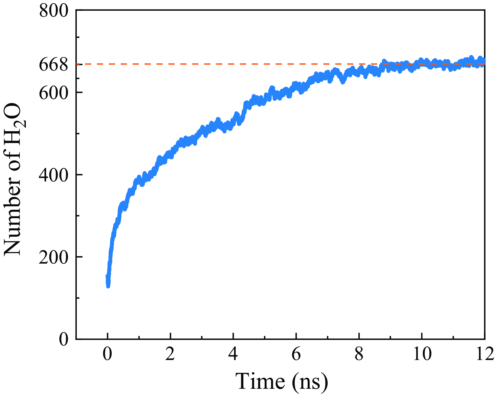
The number of water molecules inside the CNT increases over time.

We applied 1
 ${\rm atm}$
pressure to the pistons on both sides, gradually driving water molecules into the nanotube. Figure 8 shows the water molecules gradually moving inside the nanotube, reaching an equilibrium state of ∼668 water molecules inside a 50 nm nanotube after 9 ns. We then cut the CNT as an initial state of our simulation with a predefined number of water molecules. The mass density of water molecules is ∼0.85
 ${\rm g}\,{\rm m}^{-3}$
which is slightly smaller than that of the bulk water, consistent with previous studies on confined water in CNTs (Thomas & McGaughey Reference Thomas and McGaughey2008). We use
 $R_w=R- {1}/{2} \sigma _{CO}= 3.87$
Å (Fu et al. Reference Fu, Merabia and Joly2018) as the nanotube radius for mass density calculation.
Appendix B. Friction coefficient
(a) Autocorrelation function and (b) integrated friction coefficient for a four-charge-site system. (c) Autocorrelation function and (d) integrated friction coefficient of a charge-free nanotube.

The friction coefficient of the system linearly increases with the number of charged sites. The solid line is a linear fitted line to derive the friction coefficient per charged site.

The friction coefficient of nanotube systems can be calculated from the integral of the lateral force autocorrelation function at equilibrium by the Green–Kubo formula (Falk et al. Reference Falk, Sedlmeier, Joly, Netz and Bocquet2010; Bocquet & Barrat Reference Bocquet and Barrat2013):
 \begin{equation} \lambda =\frac 1{Ak_BT}\int _0^\infty {\rm d}t \langle F(t)\cdot F(0)\rangle _{{equ}}, \end{equation}
where
 $F$
is the friction force along the
 $z$
direction. We consider a (14,0) CNT, measuring systems with both a neutral surface and
 $n$
surface-bound negative charges (
 $-e$
) along with cations, where
 $n$
includes 1, 2, 4, 8 and 16. The total simulation duration was 2 ns, with autocorrelation functions
 $\langle F(t)F(0) \rangle$
calculated every 2 fs. Taking
 $n=4$
as an example, the results are shown in figure 9(a). Figure 9(b) shows the friction coefficient after integration, where the plateau values from 1 to 2 ps are averaged to determine the friction coefficient of the system. We could derive the friction coefficient of a charge-free nanotube by the autocorrelation functions as
 $\lambda _0$
= 6447.74 N s m
 $^{-3}$
as shown in figure 9(c,d). The results of the friction coefficients linearly increasing with the number of charged sites (bound ions) are shown in figure 10. We performed a linear fitting and obtained a friction coefficient of
 $\lambda _{ion}$
= 4725.33 N s m
 $^{-3}$
. Thus, the system friction coefficient as a function of bound ions (
 $N{-}n$
) is
 \begin{equation} \lambda = \lambda _0 + (N - n ) \lambda _{ion}, \end{equation}
as shown in figure 10.
The hydrodynamic friction factor
 $\alpha$
for a counterion due to the partial exposure of the ion to vacuum is numerically given by
 $\alpha = A \lambda _{ion}$
, with a value of
 $8.133 \times 10^{-13}\,{\rm N \,s\,m}^{-1}$
. This value is approximately
 $2/5$
of the classical Stokes resistance coefficient
 $6 \pi \eta a$
in bulk water using the hydration radius of the ion
 $a$
. This is possibly caused by partially dehydrated ions inside the angstrom channel, similar to the mechanism of ‘dry friction’ (Lau & Sokoloff Reference Lau and Sokoloff2024).
The fitted curve of potential of surface charge.

Appendix C. Coulomb potential well
Here we use the (14,0) CNT model as an example, where a single carbon atom was charged by
 $-e$
with a scale factor of 0.85, and a sodium ion was placed inside nanotube for a neutral system. In the equilibrium state, the sodium ion would be tightly bound to the surface charge due to strong Coulomb interaction, possibly because the bound ion is partially exposed to a vacuum-like region. We position it away from the surface charge and leave it to diffuse freely. We recorded the free energy distribution along the
 $z$
direction, which is shown as blue dots in figure 11. We averaged the raw data every 0.2 Å as a step, which is shown by the yellow points in figure 11, and fitted the potential distribution as in the form of previous work (Teber Reference Teber2005; Kavokine et al. Reference Kavokine, Marbach, Siria and Bocquet2019):
 \begin{equation} k_B T \frac {\xi }{X_T} {\rm e}^{-|x|/\xi } + C, \end{equation}
where
 $k_B$
is the Boltzmann constant,
 $T$
is the temperature and
 $\xi$
and
 $X_T$
are thermal lengths related to surrounding substance, channel shape and dielectric constants, which are not yet well understood in real systems. Ignoring the background free energy
 $C$
, we could derive the fitted parameter values:
 $\xi$
= 10.35 Å,
 $X_T$
= 0.474 Å.