



1. Introduction
Magnetohydrodynamic (MHD) channel turbulence has long been a central topic in fluid mechanics, driven by its wide-ranging applications in nuclear fusion (Abdou et al. Reference Abdou2001; Smolentsev et al. Reference Smolentsev, Moreau, Bühler and Mistrangelo2010, Reference Smolentsev, Morley, Abdou and Malang2015; Chen et al. Reference Chen, Smolentsev and Ni2020; Tran et al. Reference Tran, Stoyanov, Hauck and Smolentsev2025), electromagnetic casting and liquid-metal cooling systems. In regimes where the magnetic Reynolds number
 $\textit{Re}_m$
is much less than unity, the quasi-static approximation (Roberts Reference Roberts1967) becomes valid. Under this condition, the induced magnetic field
 $\boldsymbol{ {b}}$
is negligible compared with the externally imposed magnetic field
 $\boldsymbol{ {B}}$
, and the Lorentz force
 $\boldsymbol{ {F}}_{\textit{Lorentz}} = \boldsymbol{ {j}} \times \boldsymbol{ {B}}$
(with
 $\boldsymbol{ {j}}$
being the current density) dominates the flow dynamics. This force tends to elongate turbulent structures along the magnetic field direction, resulting in a pronounced anisotropy in the flow field.
The foundational understanding of MHD channel flows began with the seminal work of Hartmann & Lazarus (Reference Hartmann and Lazarus1937), who experimentally characterised mercury flow under transverse magnetic fields and introduced the concept of Hartmann layers. These layers exhibit a thickness scaling inversely with the Hartmann number
 $\textit{Ha}$
, and their formation is associated with suppression of wall-normal velocity gradients. Building upon this, Fraim & Heiser (Reference Fraim and Heiser1968) examined axial magnetic fields in pipe flows and reported that sufficiently strong fields could induce complete laminarisation. Later, Gardner & Lykoudis (Reference Gardner and Lykoudis1971) and Reed & Lykoudis (Reference Reed and Lykoudis1978) expanded the parameter space by analysing nonlinear drag variation and changes in Reynolds stress and turbulent kinetic energy with varying
 $\textit{Ha}$
and Reynolds numbers. To further clarify the effect of magnetic fields on flow anisotropy and structure, Branover & Gershon (Reference Branover and Gershon1979) showed that magnetic fields suppress turbulence regeneration by stretching large-scale disturbances along the field direction. However, experimental approaches have long been limited by difficulties in obtaining accurate local velocity measurements and the lack of detailed three-dimensional visualisation of turbulent structures.
To overcome these limitations, researchers increasingly turned to numerical simulations. Early numerical simulations by Lee & Choi (Reference Lee and Choi2001) used direct numerical simulation to compare the effects of magnetic fields applied in different directions, revealing that spanwise magnetic fields are more effective in reducing drag due to their direct suppression of turbulent fluctuations. In an effort to understand turbulence transition mechanisms, Krasnov et al. (Reference Krasnov, Zienicke, Zikanov, Boeck and Thess2004) emphasised the crucial role of Hartmann layer instability, a finding supported by experiments (Moresco & Alboussiere Reference Moresco and Alboussiere2004). Subsequently, Krasnov et al. (Reference Krasnov, Zikanov, Schumacher and Boeck2008) employed large-eddy simulation to examine turbulence under spanwise magnetic fields and observed significant suppression of wall-normal velocity fluctuations, which resulted in drag reduction and altered mean flow profiles.
Further refinement in numerical modelling led to investigations of more complex geometries. For example, Kobayashi (Reference Kobayashi2008) applied large-eddy simulation to high-Reynolds-number duct flows and found that, even when the Hartmann layer was laminar, turbulence could persist in sidewall regions. Building upon these insights, Krasnov et al. (Reference Krasnov, Zikanov and Boeck2012) applied high-precision methods to study duct flows at both high
 $\textit{Re}$
and
 $\textit{Ha}$
, revealing a canonical MHD flow state characterised by a laminar core and turbulent sidewalls. They further reported that in near-wall regions, velocity profiles followed a composite law combining logarithmic and linear behaviours, with the slope of the linear portion scaling with the square of magnetic induction. More recently, Doche et al. (Reference Doche, Tardu, Schillings and Capogna2021) investigated the contrasting effects of streamwise and spanwise magnetic fields on near-wall turbulence, identifying changes in quasi-coherent structures in response to field orientation.
While these studies have substantially advanced our understanding of MHD turbulence, they primarily focus on mean flow properties, friction coefficients and Reynolds stresses (Krasnov et al. Reference Krasnov, Zienicke, Zikanov, Boeck and Thess2004, Reference Krasnov, Zikanov, Schumacher and Boeck2008, Reference Krasnov, Thess, Boeck, Zhao and Zikanov2013; Boeck et al. Reference Boeck, Krasnov and Zienicke2007). In contrast, investigations into spectral dynamics – such as energy spectra, two-point correlations and interscale energy transfer – remain relatively sparse. In comparison, non-MHD (classical) channel flow research has made significant strides in this direction (Lee & Moser Reference Lee and Moser2019; Yao et al. Reference Yao, Chen and Hussain2022; Zhou et al. Reference Zhou, Xu and Jiménez2022; Chen et al. Reference Chen, Zhang, Han and Wan2024). For instance, Kim et al. (Reference Kim, Kline and Reynolds1971) and Robinson et al. (Reference Robinson1991) elucidated the role of coherent structures and streaks in near-wall turbulence. Building on this, Jiménez & Pinelli (Reference Jiménez and Pinelli1999) and Jiménez et al. (Reference Jiménez, Alamo, Juan and Flores2004) and others demonstrated that near-wall turbulence is self-sustaining and organised around ejection and sweep events, functioning independently of outer-layer turbulence.
Further spectral analysis has deepened this understanding. Studies such as those by Del Alamo & Jiménez (Reference Alamo, Juan and Jiménez2003), Lee & Moser (Reference Lee and Moser2019) and Yao et al. (Reference Yao, Chen and Hussain2022) characterised scale interactions using energy spectra, while Mizuno (Reference Mizuno2016) introduced spectral energy budget methods to reveal vertical energy transfer across wall-normal layers. Their work showed that turbulent energy extracted from large scales in the overlap region is transported both towards the channel centre and back to the near-wall region, establishing a bidirectional energy-transfer mechanism.
Despite the apparent parallels between MHD and classical turbulence, the extent to which spanwise magnetic fields modulate energy spectra and structural organisation in MHD turbulence remains poorly understood. In particular, questions about how magnetic damping alters scale-specific energy dynamics and structural lifespans remain open. The present study aims to address this gap by using direct numerical simulations to investigate the effects of spanwise magnetic fields on MHD channel turbulence. Specifically, we address the following key questions:
-
(i) Joule dissipation, unlike viscous dissipation, operates across all scales. As the strength of the spanwise magnetic field increases, how do the velocity spectra evolve? In particular, does the characteristic length scale of streamwise streaks in the near-wall region change significantly under magnetic modulation?
-
(ii) Given that near-wall streaks are a hallmark of wall-bounded turbulence, can the application of a spanwise magnetic field – through the action of the Lorentz force – alter their spatial density and temporal dynamics? If so, what are the underlying mechanisms?
-
(iii) The presence of a magnetic field is expected to reshape energy-transport processes. How does the wall-normal energy flux evolve with increasing field strength? Through which dominant mechanisms and characteristic scales does the magnetic field redistribute turbulent kinetic energy?
The structure of the remainder of this paper is as follows. In
 $\S$
2, we briefly describe the physical model and flow conditions of this study, as well as introduce the numerical algorithms, case settings and the energy spectrum budget equations. In
 $\S$
3, we discuss the main numerical results, including the energy spectrum, streamwise streaks and spectral energy budget. Finally, in
 $\S$
4, we summarise the conclusions of the study.
2. Problem statement and formulation
2.1. Governing equations and numerical method
An incompressible, pressure-driven and electrically conducting flow in a channel subjected to an external magnetic field
 $\boldsymbol{\textit {B}}$
aligned along the
 $z$
axis is considered, as shown in figure 1. Assuming the asymptotic limit of low magnetic Reynolds and Prandtl numbers, the Navier–Stokes equations for an incompressible fluid can be expressed as follows (Roberts Reference Roberts1967):
 \begin{equation} \boldsymbol{\nabla }\boldsymbol{\cdot }\boldsymbol{\textit {u}} =0, \end{equation}
 \begin{equation} \frac {\partial \boldsymbol{\textit {u}}}{\partial t}+(\boldsymbol{\textit {u}}\boldsymbol{\cdot }\boldsymbol{\nabla })\boldsymbol{\textit {u}}=-\frac {1}{\rho }\boldsymbol{\nabla }\!p+\nu \Delta \boldsymbol{\textit {u}}+\frac {\boldsymbol{\textit {j}}\times \boldsymbol{\textit {B}}}{\rho }, \end{equation}
 \begin{equation} \boldsymbol{\textit {j}}=\sigma (-\boldsymbol{\nabla }\varphi +\boldsymbol{\textit {u}}\times \boldsymbol{\textit {B}}), \end{equation}
 \begin{equation} \boldsymbol{\nabla }\boldsymbol{\cdot }\boldsymbol{\textit {j}} =0, \end{equation}
 \begin{equation} \boldsymbol{\nabla} ^2 \varphi = \boldsymbol{\nabla }\boldsymbol{\cdot }(\boldsymbol{\textit {u}}\times \boldsymbol{\textit {B}}). \end{equation}
Here,
 $\boldsymbol{ {j}}$
,
 $\varphi$
,
 $\boldsymbol{\textit {u}}$
,
 $p$
,
 $\nu$
,
 $\sigma$
and
 $\rho$
denote the current density, electric potential, velocity, pressure, kinematic viscosity, electrical conductivity and fluid density, respectively. The governing equations are numerically solved through the finite-volume method. The Poisson equation for the electric potential is then solved using a consistent and conservative scheme (Ni et al. Reference Ni, Munipalli, Huang, Morley and Abdou2007), which is verified by Chen et al. (Reference Chen, Pothérat, Ni and Moreau2021) and Wang et al. (Reference Wang, Chen, Cao, Ke, Yang and Ni2023). A Cartesian system (
 $x,y,z$
) is used here, where x axis, y axis and
 $z$
axis denote streamwise, wall-normal and spanwise directions, respectively. Two solid walls are situated at
 $y=0$
and
 $y=2h$
, with periodic boundary conditions imposed along the
 $x$
and
 $z$
directions. The physical fields are all decomposed mean and fluctuating components as
 $\varphi =\varphi +\varphi '$
, where
 $\varphi$
and
 $\varphi '$
represent the mean field and fluctuating field, respectively. Besides, the size of the numerical domain is
 $L_x\times L_y \times L_z=16 \pi h\times 2h \times 2\pi h$
. The friction Reynolds number is defined as
 \begin{equation} \textit{Re}_{\tau }=\frac {u_{\tau }h}{\nu }, \end{equation}
where
 $u_{\tau }$
is the friction velocity. Another key control parameter is the Hartmann number, defined as
 \begin{equation} Ha=Bh\sqrt {\frac {\sigma }{\rho \nu }}. \end{equation}
Sketch of the physical model.

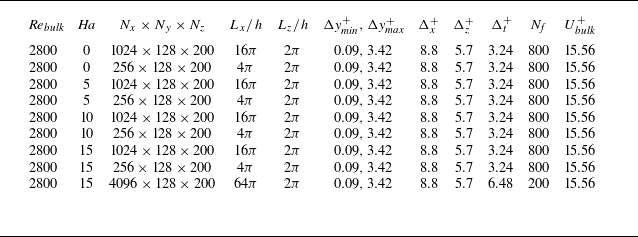
Table 1 summarises the principal parameters of the numerical simulations. The simulations are conducted under a constant-volume-flux condition, corresponding to a prescribed bulk Reynolds number
 $\textit{Re}_{\textit{bulk}}=U_{\textit{bulk}}h/\nu =2800$
, where
 $U_{\textit{bulk}}$
denotes the imposed bulk velocity. The computational grid comprises
 $N_x \times N_y \times N_z = 1024 \times 128 \times 200$
, with streamwise and spanwise spacings
 $\Delta x^+=8.8$
and
 $\Delta z^+=5.7$
, respectively. A Chebyshev-based spatial discretisation is used in the wall-normal direction with the spacing ranging from
 $\Delta y_{\textit{min}}^+=0.09$
near the wall to
 $\Delta y_{\textit{max}}^+=3.42$
at the centreline. Spectral statistics are accumulated from
 $N_{\!f}=800$
snapshots of fully developed fields. At
 $\textit{Ha}=20$
the flow has fully relaminarised; accordingly, the discussion is restricted to
 $\textit{Ha}=0,\ 5,\ 10$
and
 $15$
.
Simulation parameters. Here,
 $L_x$
and
 $L_z$
are the streamwise and spanwise dimensions of the computational domain, respectively, and
 $h$
is the channel half-height;
 $\Delta x$
and
 $\Delta z$
represent the streamwise and spanwise grid resolutions, while
 $\Delta y_{\textit{min}}$
and
 $\Delta y_{\textit{max}}$
are the finest and coarsest wall-normal grid spacings;
 $N_x$
,
 $N_y$
and
 $N_z$
are the number of collocation points in the streamwise, wall-normal and spanwise directions;
 $\Delta t^+$
denotes the average time interval between stored fields in viscous units, and
 $N_{\!f}$
is the number of fully developed fields used for post-processing, after the initial transients have been removed; and
 $U^+_{\textit{bulk}}$
represents the imposed non-dimensional bulk velocity. All wall-unit quantities are non-dimensionalised using the nominal friction Reynolds number
 $\textit{Re}_\tau =180$
for scaling purposes.

Table 1. Long description
A table summarizing parameters of numerical simulations. The table has 8 rows and 14 columns. Column headers are Re_bulk, Ha, N_x x N_y x N_z, L_x/h, L_z/h, Δy^+/Δy^+_max, Δx^+, Δz^+, Δt^+, N_f, U^+_bulk. Row 1: Re_bulk, 2800; Ha, 0; N_x x N_y x N_z, 1024 x 128 x 200; L_x/h, 16π; L_z/h, 2π; Δy^+_min, 0.09; Δy^+_max, 3.42; Δx^+, 8.8; Δz^+, 5.7; Δt^+, 3.24; N_f, 800; U^+_bulk, 15.56. Row 2: Re_bulk, 2800; Ha, 0; N_x x N_y x N_z, 256 x 128 x 200; L_x/h, 4π; L_z/h, 2π; Δy^+_min, 0.09; Δy^+_max, 3.42; Δx^+, 8.8; Δz^+, 5.7; Δt^+, 3.24; N_f, 800; U^+_bulk, 15.56. Row 3: Re_bulk, 2800; Ha, 5; N_x x N_y x N_z, 1024 x 128 x 200; L_x/h, 16π; L_z/h, 2π; Δy^+_min, 0.09; Δy^+_max, 3.42; Δx^+, 8.8; Δz^+, 5.7; Δt^+, 3.24; N_f, 800; U^+_bulk, 15.56. Row 4: Re_bulk, 2800; Ha, 5; N_x x N_y x N_z, 256 x 128 x 200; L_x/h, 4π; L_z/h, 2π; Δy^+_min, 0.09; Δy^+_max, 3.42; Δx^+, 8.8; Δz^+, 5.7; Δt^+, 3.24; N_f, 800; U^+_bulk, 15.56. Row 5: Re_bulk, 2800; Ha, 10; N_x x N_y x N_z, 1024 x 128 x 200; L_x/h, 16π; L_z/h, 2π; Δy^+_min, 0.09; Δy^+_max, 3.42; Δx^+, 8.8; Δz^+, 5.7; Δt^+, 3.24; N_f, 800; U^+_bulk, 15.56. Row 6: Re_bulk, 2800; Ha, 10; N_x x N_y x N_z, 256 x 128 x 200; L_x/h, 4π; L_z/h, 2π; Δy^+_min, 0.09; Δy^+_max, 3.42; Δx^+, 8.8; Δz^+, 5.7; Δt^+, 3.24; N_f, 800; U^+_bulk, 15.56. Row 7: Re_bulk, 2800; Ha, 15; N_x x N_y x N_z, 1024 x 128 x 200; L_x/h, 16π; L_z/h, 2π; Δy^+_min, 0.09; Δy^+_max, 3.42; Δx^+, 8.8; Δz^+, 5.7; Δt^+, 3.24; N_f, 800; U^+_bulk, 15.56. Row 8: Re_bulk, 2800; Ha, 15; N_x x N_y x N_z, 4096 x 128 x 200; L_x/h, 64π; L_z/h, 2π; Δy^+_min, 0.09; Δy^+_max, 3.42; Δx^+, 8.8; Δz^+, 6.48; Δt^+, 3.24; N_f, 200; U^+_bulk, 15.56.
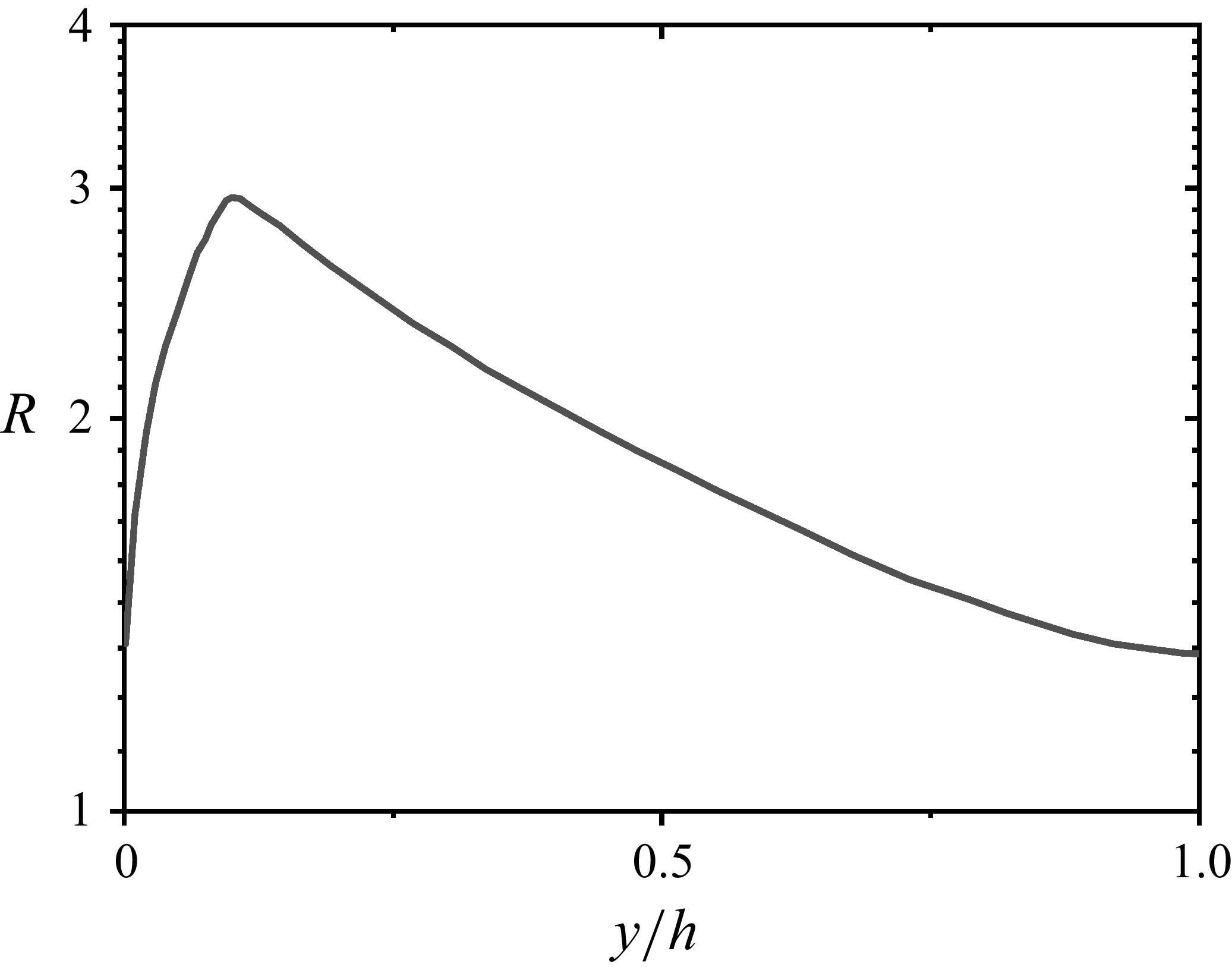
To assess the grid resolution, we adopt the evaluation procedure of Vreman & Kuerten (Reference Vreman and Kuerten2014) and Pont-Vílchez et al. (Reference Pont-Vílchez, Trias, Gorobets and Oliva2019) for direct numerical simulations. The effective grid scale
 $\varDelta$
is defined as the cube root of the local cell volume:
 \begin{equation} \varDelta = (\Delta _x \Delta _y \Delta _z)^{1/3}. \end{equation}
Grid-quality assessment: ratio of the effective grid scale to the Kolmogorov scale at different wall-normal locations.

We then compare
 $\varDelta$
with the Kolmogorov scale
 $\eta$
(with
 $\eta = (\nu ^3 / \epsilon )^{0.25}$
) and form their ratio
 $R=\Delta /\eta$
. Figure 2 shows the wall-normal distribution of
 $R$
, which remains below 3 everywhere, meeting conventional direct numerical simulation resolution criteria. Moreover, for the
 $\textit{Ha}=0$
case the simulation yields
 $\textit{Re}_\tau =178.4$
, deviating from the nominal value
 $\textit{Re}_{\tau }=180$
by less than
 $1\,\%$
, further corroborating that the grid resolution is sufficiently fine.
2.2. Spectral energy budget equation
The budget equation for turbulent kinetic energy
 $e=(u'^2+v'^2+w'^2)/2$
is given by
 \begin{equation} \frac { \partial \bar {e}}{\partial t} = P + T + T_p + \epsilon _{\nu } + D_{\nu } + \epsilon _{j}. \end{equation}
Here, the overbar stands for averaging over two homogeneous directions (
 $x$
direction and
 $z$
direction) and time. For channel flow, the mean velocity has a non-zero component only in the streamwise direction, which depends on
 $y$
and is denoted by
 $U(y)$
hereafter. Since the flow is statistically steady, the left-hand side of (2.9) reduces to
 $0$
, leading to an equilibrium between the terms on the right-hand side. The terms
 $P$
,
 $T$
,
 $T_p$
,
 $\epsilon _{nu}$
,
 $D_{\nu }$
and
 $\epsilon _{\!j}$
represent the production rate of the turbulent kinetic energy, the spatial turbulent transport, the transport of energy by the turbulent pressure gradient, the dissipation rate, the viscous diffusion and the Joule dissipation rate, respectively. All the terms on the right-hand side of (2.9) are expressed as
 \begin{equation} \left . \begin{aligned} P(y) = -\overline {u'v'} \frac {\text{d}U}{\text{d}y},\quad T (y) = -\frac {\text{d}\overline {ev'}}{\text{d}y}, \quad T_p(y) = -\frac {1}{\rho } \frac {\text{d}\overline {p' v'}}{\text{d}y}, \\[11pt] \varepsilon _{\nu }(y) = -\nu \overline {\left ( \frac {\partial u'_{\!j}}{\partial x_k} \frac {\partial u'_{\!j}}{\partial x_k}\right ) },\quad D_{\nu }(y) = \nu \frac {\text{d}^2 \overline {e}}{\text{d}y^2},\quad \varepsilon _{j}=\sigma B \overline {\frac {\partial \varphi '}{\partial x} v'} - \sigma B \overline {\frac {\partial \varphi '}{\partial y} u'} - \sigma B^2 \big ( \overline {u'^2} + \overline {v'^2} \big ). \end{aligned} \right \} \end{equation}
Here, summation is implied over the same index. Due to the homogeneity in the wall-parallel directions, net spatial transport is observed solely in the
 $y$
direction, as illustrated by the terms
 $T$
,
 $T_p$
and
 $D_{\nu }$
. To better investigate the influence of the magnetic field, we further decompose the MHD term into two source components (
 $S_1$
and
 $S_2$
) and one annihilation component (
 $A$
) (Doche et al. Reference Doche, Tardu, Schillings and Capogna2021), with the specific definitions as follows:
 \begin{equation} S_1= - \sigma B \overline {\frac {\partial \varphi '}{\partial y} u'},\quad S_2=\sigma B \overline {\frac {\partial \varphi '}{\partial x} v'},\quad A= - \sigma B^2 \big ( \overline {u'^2} + \overline {v'^2}\big ). \end{equation}
Due to the homogeneity in
 $x$
and
 $z$
directions, we study the spectra (2.9) within each wall-parallel plane. According to Lumley (Reference Lumley1964) and Mizuno (Reference Mizuno2016), the spectral equation is derived through the Fourier modes of velocity, pressure and electric potential fluctuations ((
 $\hat {u'}(\boldsymbol{\textit {k}},y),\hat {v'}(\boldsymbol{\textit {k}},y),\hat {w'}(\boldsymbol{\textit {k}},y)), \hat {p'}(\boldsymbol{\textit {k}},y),\hat {\phi '}(\boldsymbol{\textit {k}},y)$
), where the hat represents Fourier transform which is transformed only in
 $x$
and
 $z$
directions, and
 $\boldsymbol{\textit {k}}=(k_x,k_z)$
is the wavenumber in Fourier space. For brevity,
 $\hat {u'}(\boldsymbol{k}, y)$
,
 $\hat {v'}(\boldsymbol{k}, y)$
,
 $\hat {w'}(\boldsymbol{k}, y)$
,
 $\hat {p'}(\boldsymbol{k}, y)$
and
 $\hat {\varphi '}(\boldsymbol{k}, y)$
will hereafter be written as
 $\hat {u'}$
,
 $\hat {v'}$
,
 $\hat {w'}$
,
 $\hat {p'}$
and
 $\hat {\varphi '}$
. The spectral equation of the energy budget is given by
 \begin{equation} \frac {\partial \tilde {e}}{\partial t} = \tilde {P} + \tilde {T} + \tilde {T}_p + \tilde {\varepsilon }_{\nu } + \tilde {D}_{\nu } + \tilde {T}^s+\tilde {\varepsilon }_{\!j}, \end{equation}
where
 \begin{align} \tilde {P}(\boldsymbol{\textit {k}}, y) &= \textit{Re} \left \{ - \left \langle \widehat {u'} \widehat {v'}^* \frac {\text{d}U}{\text{d}y} \right \rangle \right \}\!, \\[-12pt]\nonumber \end{align}
 \begin{align} \tilde {T}(\boldsymbol{\textit {k}}, y) &= \textit{Re} \left \{ - \frac {1}{2} \frac {\text{d}}{\text{d}y} \big \langle \widehat {u'_{\!j}} \widehat {(u'_{\!j} v)}^* \big \rangle \right \}\!, \\[0pt]\nonumber \end{align}
 \begin{align} \tilde {T}_p(\boldsymbol{\textit {k}}, y) &= \textit{Re} \left \{ - \frac {1}{\rho } \frac {\text{d}}{\text{d}y} \Big \langle \widehat {p^{\prime *}} \hat {v'} \Big \rangle \right \}\!, \\[-12pt]\nonumber \end{align}
 \begin{align} \tilde {\varepsilon }_{\nu }(\boldsymbol{\textit {k}}, y) &= -2\nu \big(k_x^2 + k_z^2 \big) \tilde {e} - \nu \left \langle \left | \frac {\text{d} \widehat {u'_{\!j}}}{\text{d}y} \right |^2 \right \rangle \!, \\[-12pt]\nonumber \end{align}
 \begin{align} \tilde {D}_{\nu }(\boldsymbol{\textit {k}}, y) &= \nu \frac {\text{d}^2 \tilde {e}}{\text{d}y^2}, \\[-12pt]\nonumber \end{align}
 \begin{align} \tilde {T}^s(\boldsymbol{\textit {k}}, y) &= \textit{Re} \left \{ \Big \langle \partial _k \widehat {u'_{\!j}} (\widehat {u'_{\!j} u'_k})^* \Big \rangle - \frac {1}{2} \frac {\text{d}}{\text{d}y} \Big \langle \widehat {u'_{\!j}} (\widehat {u'_{\!j} v'})^* \Big \rangle \right \} \!, \\[-12pt]\nonumber \end{align}
 \begin{align} \tilde {S}_1(\boldsymbol{\textit {k}}, y) &= \textit{Re} \left \{ - \left \langle \sigma B \widehat {u'}^* \frac {\partial \widehat {\varphi '} }{\partial y} \right \rangle \right \}\!, \\[-12pt]\nonumber \end{align}
 \begin{align} \tilde {S}_2(\boldsymbol{\textit {k}}, y) &= \textit{Re} \Big \{ \Big \langle ik_x \sigma B \widehat {v'}^* \widehat {\varphi '} \Big \rangle \Big \}, \\[-12pt]\nonumber \end{align}
 \begin{align} \tilde {A}(\boldsymbol{\textit {k}}, y) &= \textit{Re} \Big \{ \sigma B^2 \Big \langle \widehat {u'} \widehat {u'}^* + \widehat {v'} \widehat {v'}^* \Big \rangle \Big \} \end{align}
and
 $(\partial _1,\partial _2,\partial _3)=(ik_x, \partial /\partial y,ik_z)$
. The asterisk denotes the complex conjugate. The angle brackets denote averaging in time and the tilde denotes the Fourier-transformed (spectral) counterpart of each physical-space term in the budget equation. The terms in (2.13)–(2.21) of the spectral budget equation (2.12) represent the respective spectral or cospectral decompositions of the corresponding terms on the right-hand side of (2.9). The term
 $\tilde {T}^s$
in (2.18) denotes the energy transport between scales, which does not contribute to the overall budget (2.9) due to
 $\varSigma _k \tilde {T}^s(\boldsymbol{\textit {k}},y)=0$
for any
 $y$
.
The spectra and cross-spectra in (2.13)–(2.21) provide scale information confined to the
 $x$
–
 $z$
plane, without capturing the detailed characteristics of scales in the wall-normal direction. Although investigating wall-normal scale dynamics and energy transport is crucial for a deeper understanding of the physical mechanisms of wall-bounded turbulence, these aspects lie beyond the scope of the present study. For detailed analyses of energy transport in the wall-normal direction, the reader is referred to the work of Cimarelli et al. (Reference Cimarelli, De Angelis, Schlatter, Brethouwer, Talamelli and Casciola2015), Chen & Vassilicos (Reference Chen and Vassilicos2022) and Apostolidis et al. (Reference Apostolidis, Laval and Vassilicos2023)
3. Results and discussion
3.1. Mean flow
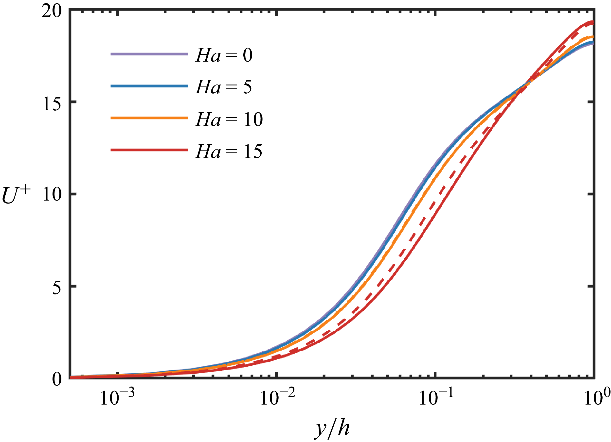
Figure 3 presents the mean-velocity profiles
 $U_M$
under different
 $\textit{Ha}$
. As
 $\textit{Ha}$
increases, the near-wall velocity gradient diminishes, evidencing the suppressive influence of the magnetic field on the flow.
Mean-velocity profiles for a spanwise magnetic field at various
 $\textit{Ha}$
. Solid lines correspond to the computational domain
 $16\pi \times 2\times 2\pi$
, and dashed lines to
 $4\pi \times 2\times 2\pi$
. All quantities are non-dimensionalised by
 $u_\tau$
.

Distributions of (a) streamwise fluctuation
 $\langle u'u'\rangle ^{1/2}$
, (b) wall-normal fluctuation
 $\langle v'v'\rangle ^{1/2}$
, (c) spanwise fluctuation
 $\langle w'w'\rangle ^{1/2}$
and (d) Reynolds shear stress
 $\langle u'v'\rangle$
at different wall-normal positions for a spanwise magnetic field at various
 $\textit{Ha}$
. Solid lines:
 $16\pi \times 2\times 2\pi$
; dashed lines:
 $4\pi \times 2\times 2\pi$
. All quantities are non-dimensionalised by
 $u_\tau$
.

Figure 4. Long description
Four line graphs illustrate the distributions of different fluctuations and Reynolds shear stress at various wall-normal positions under a spanwise magnetic field. Panel A: The line graph shows the streamwise fluctuation with the y-axis labeled as the square root of the streamwise fluctuation and the x-axis labeled as the wall-normal position normalized by height. Solid lines represent one set of values, while dashed lines represent another. Panel B: The line graph displays the wall-normal fluctuation with the same axes and line styles as Panel A. Panel C: The line graph presents the spanwise fluctuation with identical axes and line styles. Panel D: The line graph illustrates the Reynolds shear stress with the same axes and line styles. Each graph includes multiple lines corresponding to different magnetic field strengths, showing how these fluctuations and stress vary with wall-normal position and magnetic field strength.
A closer inspection shows that once
 $\textit{Ha}\geqslant 10$
, the mean-velocity profiles exhibit pronounced domain-size dependence. The same tendency appears in the turbulence intensities and Reynolds stresses (see figure 4). All results are obtained by long-time averaging after the flow has reached a statistically stationary state. The discrepancies between the two domains primarily arise from magnetic-field-induced elongation of near-wall quasi-organised structures, which the smaller domain
 $4\pi \times 2\times 2\pi$
cannot adequately capture (see § 3.2) (Jiménez & Moin Reference Jiménez and Moin1991). Because these large-scale structures are intimately tied to turbulence production and energy transport, the smaller domain can bias statistics such as the mean and fluctuating velocities. Consequently, we employed the larger computational domain
 $16\pi \times 2 \times 2\pi$
and found its results to be in close agreement with those from
 $32\pi \times 2 \times 2\pi$
. Hence, the subsequent analysis relies on the
 $16\pi \times 2\times 2\pi$
domain.
Figure 4 further shows the turbulence intensities and Reynolds stresses at different
 $\textit{Ha}$
. Overall, both diminish as
 $\textit{Ha}$
increases. However, for the
 $16\pi \times 2\times 2\pi$
domain at
 $\textit{Ha}=15$
, the streamwise fluctuation
 $\langle u'\rangle$
rises markedly for
 $y/h\gt 0.3$
, even exceeding its zero-magnetic-field level – an observation that runs counter to the intuitive expectation of universal magnetic suppression. Notably, Zikanov et al. (Reference Zikanov, Krasnov, Boeck and Sukoriansky2019) reported a related phenomenon for honeycomb jets, where turbulent kinetic energy near a pipe centre increased with stronger magnetic fields. The underlying mechanism of this effect will be examined in subsequent sections.
3.2. Energy spectrum
3.2.1. The modulation of the energy spectrum by the magnetic field
Building upon established methodologies from previous studies (Kim & Adrian Reference Kim and Adrian1999; Guala et al. Reference Guala, Hommema and Adrian2006; Lee & Moser 2015, Reference Lee and Moser2019; Duan et al. Reference Duan, Chen, Li and Zhong2020; Yao et al. Reference Yao, Chen and Hussain2022), this research employs one-dimensional velocity spectra to elucidate the scale-wise distribution of turbulent kinetic energy and Reynolds shear stress, aiming to offer deeper insights into the modulation of turbulent structures induced by magnetic fields. We first present the definition of the velocity-spectrum tensor as follows (Pope Reference Pope2001):
 \begin{equation} \phi _{u_i u_{\!j}}(\boldsymbol{k},y) = \hat {R}_{u_i u_{\!j}} (\boldsymbol{k},y) = \langle \hat {u}_i(\boldsymbol{k},y) \hat {u}_{\!j}(\boldsymbol{k},y) \rangle .\end{equation}
Premultiplied spectra of streamwise velocity
 $k_x\varSigma _{k_z}\phi _{uu}/u_{\tau }^2$
as a function of
 $\lambda _x^+$
and
 $y^+$
for: (a)
 $\textit{Ha}=0$
, (b)
 $\textit{Ha}=5$
, (c)
 $\textit{Ha}=10$
and (d)
 $\textit{Ha}=15$
.

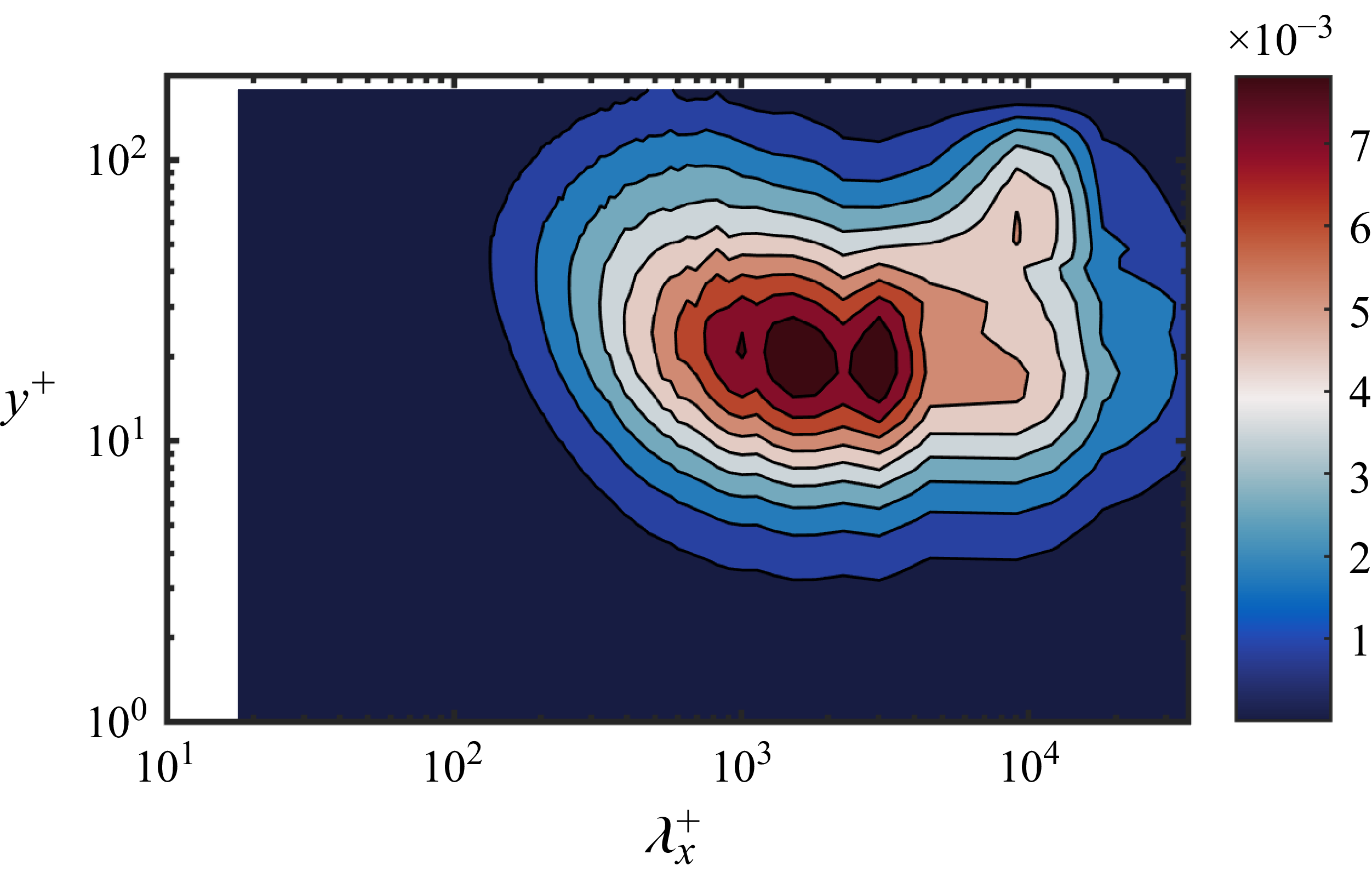
Premultiplied spectra of streamwise velocity
 $k_x\varSigma _{k_z}\phi _{uu}/u_{\tau }^2$
as a function of
 $\lambda _x^+$
and
 $y^+$
at
 $\textit{Ha}=15$
for the domain
 $L_x \times L_y \times L_z = 64\pi \times 2 \times 2\pi$
.

For the sake of clarity, the velocity-spectrum tensor will hereafter be simplified to
 $\phi _{u_i u_{\!j}}$
. Figure 5 presents the premultiplied one-dimensional spectra of the streamwise velocity fluctuations,
 $k_x\varSigma _{k_z}\phi _{uu}/u_{\tau }^2$
, illustrating the distribution as a function of streamwise wavelength
 $\lambda _x$
and wall-normal coordinate
 $y^+$
at various Hartmann numbers. Under non-magnetic conditions (
 $\textit{Ha} = 0$
), a pronounced spectral peak is evident at approximately
 $y^+ \approx 14$
near the wall, characterised by a representative streamwise length scale of
 $\lambda _x^+ \approx 1000$
, aligning remarkably well with classical findings in the literature (Waleffe Reference Waleffe1997; Schoppa & Hussain Reference Schoppa and Hussain2002; Morrison et al. Reference Morrison, Jiang, McKeon and Smits2002; Lee & Moser Reference Lee and Moser2015), thus further confirming the reliability of our numerical simulations. As the magnetic field strength increases, the characteristic length of the near-wall streaks extends markedly: from
 $\lambda _x^+\approx 1000$
at
 $\textit{Ha}=0$
to
 $\lambda _x^+\approx 1800$
at
 $\textit{Ha}=15$
. Under the strong-field condition (
 $\textit{Ha}=15$
), a distinct secondary near-wall peak emerges at
 $\lambda _x^+\approx 3000$
, suggesting the onset of an altered dynamical regime. Concurrently, the wall-normal location of the primary peak shifts outward (from
 $y^+\approx 14$
to
 $y^+\approx 22$
), indicating that the field substantially reorganises the loci and spatial distribution of turbulent kinetic energy input. For
 $\textit{Ha}=15$
, a new spectral peak also manifests in the outer layer (
 $y^+ \gt 40$
) at streamwise scales. It is worth noting, however, that due to the constraints of the computational domain, this peak remains indistinct; we therefore extended the domain to
 $L_x \times L_y \times L_z = 64\pi \times 2 \times 2\pi$
. As shown in figure 6, a fully developed peak emerges in the outer region at
 $\lambda _x \approx 8000$
, strongly suggesting the formation of very large-scale motions (Kim & Adrian Reference Kim and Adrian1999; Balakumar & Adrian Reference Balakumar and Adrian2007; Cameron et al. Reference Cameron, Nikora and Stewart2017; Yao et al. Reference Yao, Chen and Hussain2022). The advent of these outer-layer superstructures coincides with the marked increase in turbulent kinetic energy observed at
 $\textit{Ha}=15$
; we conjecture that the magnetic field impedes the downscale transfer of energy, thereby promoting upscale transport. To the best of our knowledge, this constitutes the first observation of such outer-layer large-scale structures at so low a Reynolds number.
Figure 7 further illustrates the premultiplied one-dimensional spanwise energy spectra of streamwise velocity fluctuations,
 $k_z \varSigma _{k_x}\phi _{uu}/u_\tau ^2$
, across varying Hartmann numbers. At
 $\textit{Ha} = 0$
, a prominent spectral peak emerges around the buffer layer at
 $y^+ \approx 14$
, corresponding to a characteristic spanwise wavelength of approximately
 $\lambda _z^+ \approx 100$
, aligning closely with the traditional near-wall streak scale. As
 $\textit{Ha}$
increases, the spanwise scale of near-wall streamwise streaks expands moderately from
 $\lambda _z^+ \approx 100$
at
 $\textit{Ha} = 0$
to around
 $\lambda _z^+ \approx 130$
at
 $\textit{Ha} = 15$
. Notably, however, this increase is substantially less pronounced compared with the growth observed in the streamwise scale (
 $\lambda _x$
), thereby challenging the conventional intuition that turbulent structures would elongate significantly along the magnetic field direction (spanwise) under the influence of Lorentz forces. It is also noteworthy that under
 $\textit{Ha}=15$
, only a single, distinct energy peak appears in the spanwise spectrum, indicating a convergence towards a uniform characteristic spanwise structure.
Premultiplied spectra of streamwise velocity
 $k_z\varSigma _{k_x}\phi _{uu}/u_{\tau }^2$
as a function of
 $\lambda _z^+$
and
 $y^+$
for: (a)
 $\textit{Ha}=0$
and (b)
 $\textit{Ha}=15$
.

Premultiplied spectra of Reynolds stress
 $k_x\varSigma _{k_z}\phi _{uv}/u_{\tau }^2$
as a function of
 $\lambda _x^+$
and
 $y^+$
for: (a)
 $\textit{Ha}=0$
, (b)
 $\textit{Ha}=5$
, (c)
 $\textit{Ha}=10$
and (d)
 $\textit{Ha}=15$
.

Figure 8. Long description
Panel A: A heat map showing premultiplied spectra of Reynolds stress as a function of y+ and λx+. The x-axis represents λx+ ranging from 10^1 to 10^3, and the y-axis represents y+ ranging from 10^0 to 10^2. The color scale ranges from 1 to 7 times 10^-4, with darker colors indicating lower values and lighter colors indicating higher values. The heat map shows a central concentration of higher values. Panel B: A heat map similar to Panel A, with the same axes and color scale. The distribution of values is slightly different, showing a slightly shifted central concentration. Panel C: A heat map similar to Panel A, with the same axes and color scale. The distribution of values is slightly different, showing a slightly shifted central concentration. Panel D: A heat map similar to Panel A, with the same axes and color scale. The distribution of values is slightly different, showing a slightly shifted central concentration.
Immediately following, figure 8 presents the one-dimensional streamwise premultiplied energy spectrum of the Reynolds stress,
 $ k_x \varSigma _{k_z}\phi _{uv} / u_{\tau }^2$
, under varying Hartmann numbers. It is noteworthy that in the near-wall region, the modulation of the Reynolds stress by the magnetic field mirrors that of the streamwise velocity fluctuations. As the magnetic field strength increases, the streamwise direction corresponding to the peak value of the Reynolds stress in the near-wall region also grows. Furthermore, when the Hartmann number reaches
 $\textit{Ha} = 15$
, two distinct peaks emerge in the spectrum, aligning with the two peaks in the streamwise velocity fluctuation spectrum. This suggests that the energy of the near-wall double-peak phenomenon is injected by the mean flow. In contrast to the streamwise velocity spectrum
 $ k_x\varSigma _{k_z} \phi _{uu}$
, no new energy peak in the outer layer is observed here, indicating that the intensified field does not significantly reorganise the outer-layer Reynolds stress. Consequently, the very large-scale structures in the outer region arise from an upscale (inverse-cascade) energy transfer.
3.2.2. The influence of the magnetic field on large-scale structures
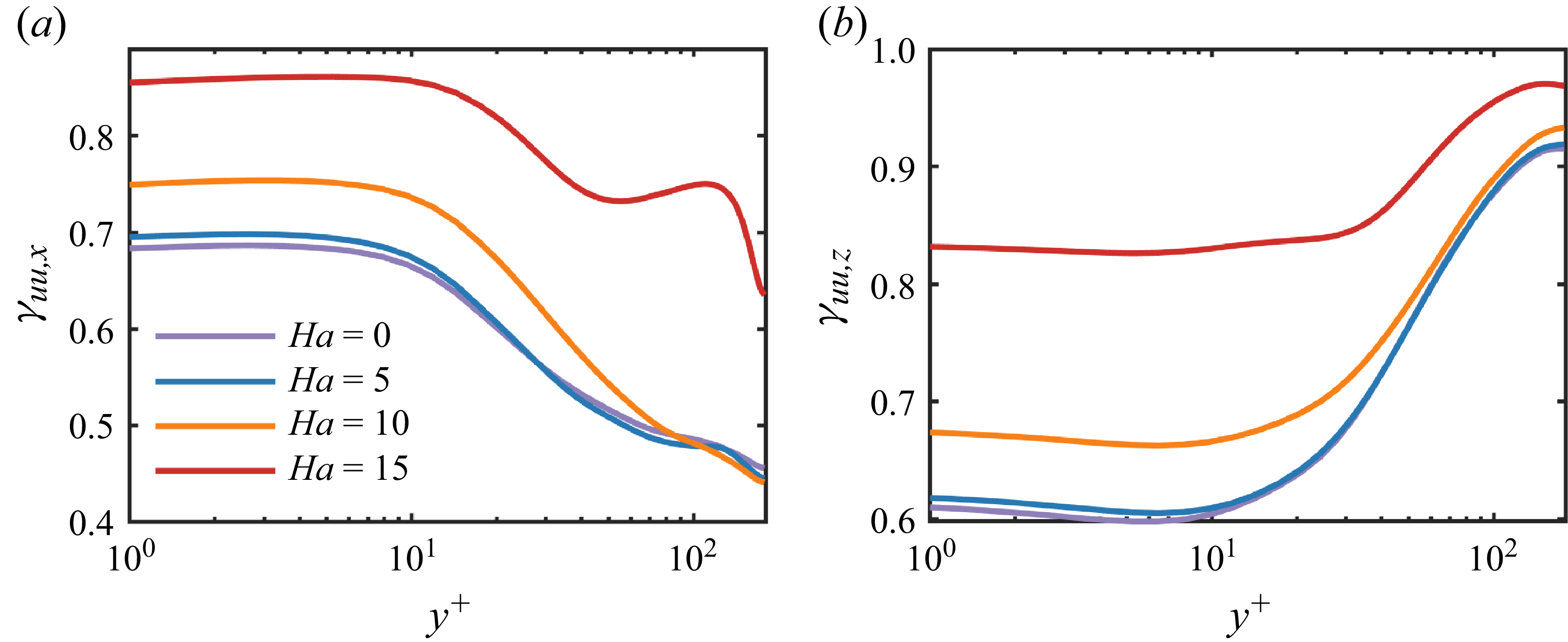
Figure 9(b) presents the spanwise-component results. In contrast to the streamwise large-scale energy distribution, the spanwise large-scale fraction is maximal in the outer layer, a behaviour closely linked to the Lorentz-force source term present there; a detailed analysis is provided in § 3.4. With increasing magnetic field strength, the spanwise large-scale energy strengthens overall; notably, at
 $\textit{Ha}=15$
the near-wall fraction also rises markedly. Unlike the pronounced non-monotonic variations observed for the streamwise energy in the outer layer, the spanwise counterpart grows more gently, indicating a comparatively weaker magnetic control over outer-layer spanwise structures. From an energetic perspective, the principal field-induced dissipation term is
 $\sigma B^2(u^2+v^2)$
. As the magnetic field strength increases, the turbulent kinetic energy tends to concentrate in large-scale structures and is primarily dissipated via Joule dissipation.
The fraction of streamwise kinetic energy carried by large scales defined on (a)
 $k_x \lt 10$
and (b)
 $k_z \lt 10$
.

To further elucidate the variation in large-scale energy induced by the magnetic field, we conducted an integrated analysis of turbulent kinetic energy in wavenumber space, following methodologies proposed by Balakumar & Adrian (Reference Balakumar and Adrian2007), Duan et al. (Reference Duan, Chen, Li and Zhong2020) and Yao et al. (Reference Yao, Chen and Hussain2022). The integration expression is defined as
 \begin{equation} \gamma _{u_iu_{\!j},x}(k_c) = \frac {\int _0^{k_c}\varSigma _{k_z}\phi _{u_iu_{\!j}} {\rm d}k_x}{\int _0^{\infty } \varSigma _{k_z}\phi _{u_iu_{\!j}} {\rm d}k_x} ,\quad \gamma _{u_iu_{\!j},z}(k_c) = \frac {\int _0^{k_c}\varSigma _{k_x}\phi _{u_iu_{\!j}} {\rm d}k_z}{\int _0^{\infty }\varSigma _{k_x}\phi _{u_iu_{\!j}} {\rm d}k_z}, \end{equation}
where
 $k_c = 10$
represents the cutoff wavenumber employed to distinguish large-scale energy. We selected a friction Reynolds number of
 $\textit{Re}_{\tau } = 180$
, which, while insufficient to support the formation of typical large-scale motions and very large-scale motions (Yao et al. Reference Yao, Chen and Hussain2022), remains adequate to capture and demonstrate the modulation trends of large-scale structures and their energy content due to magnetic field variations.
Figure 9(a) shows the
 $y^+$
dependence of the streamwise large-scale turbulent kinetic energy across Hartmann numbers. In the absence of a magnetic field (
 $\textit{Ha}=0$
), the near-wall fraction of large-scale energy is maximal – about
 $68\,\%$
– indicating that this region is dominated by streamwise streaks. With increasing wall distance, the fraction declines, reaching roughly half its near-wall level at the channel centre. As the magnetic field intensifies – most notably at
 $\textit{Ha}=15$
– the near-wall fraction rises sharply to
 ${\approx}85\,\%$
, evidencing strong suppression of small-scale energy production and growth. In the outer layer, the trends diverge with
 $\textit{Ha}$
. For
 $\textit{Ha}=5$
and
 $\textit{Ha}=10$
, the decay closely tracks that at
 $\textit{Ha}=0$
. Under the strongest field (
 $\textit{Ha}=15$
), however, a distinctly non-monotonic pattern emerges – decrease, then increase, then decrease – while still sustaining a comparatively high value of about
 $68\,\%$
near the opposite wall. This behaviour is consistent with the outer-layer spectral peak in figure 5(d) and further indicates that the magnetic field markedly reshapes turbulence-energy transport, promoting upscale (inverse) transfer (Baker et al. Reference Baker, Pothérat, Davoust and Debray2018; Fan et al. Reference Fan, Chen and Ni2025).
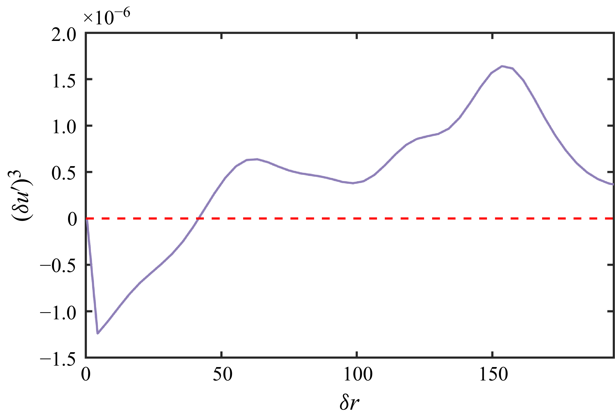
To further investigate this mechanism, we examine the third-order structure function of the streamwise velocity in the outer region. Given that turbulent kinetic energy production is negligible there and the flow is statistically homogeneous in the streamwise direction, the third-order structure function serves as a suitable indicator of energy transfer direction. Figure 10 shows this function for the streamwise velocity fluctuations at
 $y^+ \approx 140$
; its sign denotes the transfer direction (positive for forward, negative for inverse). The results reveal clear bidirectional energy transfer, consistent with Baker et al. (Reference Baker, Pothérat, Davoust and Debray2018), Fan et al. (Reference Fan, Chen and Ni2025) and Klein & Pothérat (Reference Klein and Pothérat2010). Moreover, the magnitude of the inverse energy transfer is significantly larger than that of the forward transfer, suggesting that the emergence of large-scale structures in the outer region is primarily attributable to the inverse energy transfer.
The streamwise third-order structure function
 $(\delta u')^3(r)$
as a function of
 $r$
at
 $y^+ \approx 140$
for
 $\textit{Ha}=15$
, obtained in the domain
 $L_x \times L_y \times L_z = 64\pi \times 2 \times 2\pi$
. Results are averaged over
 $N_{\!f}=200$
snapshots and over both half-planes by exploiting statistical symmetry, with a mild Gaussian smoothing applied for visualisation.

3.2.3. Dual peak in energy spectrum in near-wall region at high
 $\textit{Ha}$

To further interrogate the near-wall double-peak phenomenon in figure 5(d), figure 11 displays instantaneous isocontours of the velocity fluctuation at
 $y^+=20$
. Two canonical flow states are clearly discernible: first, a high-momentum regime composed of alternating high- and low-speed streaks, with a characteristic streamwise scale
 $\lambda _x\approx 10h$
(i.e.
 $\lambda _x^+\approx 1800$
), corresponding to the first peak in figure 5(d); and second, a low-momentum regime dominated by low-speed streaks of scale
 $\lambda _x\approx 20h$
, associated with the second peak. These structures are distributed highly unevenly in space, with both streak density and intensity markedly greater in the high-momentum regions. It is worth noting that this closely resembles the laminar–turbulent coexistence zone identified by Brethouwer et al. (Reference Brethouwer, Duguet and Schlatter2012).
Instantaneous snapshots of
 $u'$
at
 $y^+=20$
and
 $\textit{Ha}=15$
.

Time evolution of integrated kinetic turbulent energy in the lower half-plane for (a)
 $\textit{Ha}=0$
, (b)
 $\textit{Ha}=5$
, (c)
 $\textit{Ha}=10$
and (d)
 $\textit{Ha}=15$
.

Figure 12 displays the temporal evolution of lower-half-plane integrated streamwise turbulent kinetic energy
 $q$
at a specific cross-section for different Hartmann numbers. Here,
 $q$
is defined as
 \begin{equation} q=\int u'^2 \,{\rm d} A, \end{equation}
where
 $A$
denotes the area of the lower half (
 $y \leqslant h$
) of an arbitrary
 $y$
–
 $z$
cross-section at a fixed streamwise location
 $x$
, spanning the full spanwise extent
 $0 \leqslant z \leqslant L_z$
. Owing to the statistical symmetry between the upper and lower halves of the channel, only the lower half-plane is analysed. To more precisely characterise the fluctuating energy dynamics, we computed the standard deviation coefficient
 $\lambda = \sigma / \mu$
of turbulent kinetic energy under various magnetic field conditions, yielding values of
 $0.0148$
,
 $0.0152$
,
 $0.1504$
and
 $0.3178$
, where
 $\sigma$
is the standard deviation and
 $\mu$
is the mean turbulent kinetic energy. At
 $\textit{Ha}=0$
and
 $\textit{Ha}=5$
, turbulent kinetic energy fluctuates around the mean with slight variations. As the magnetic field intensity increases, the fluctuation amplitude of turbulent kinetic energy gradually intensifies. This phenomenon can be attributed to the additional energy dissipation mechanisms introduced by the magnetic field, namely the competition between Lorentz forces and inertial forces. Under strong-magnetic-field conditions (
 $\textit{Ha}=15$
), a distinct contrast in turbulent kinetic energy between the high- and low-momentum regions is observed in figure 11. This behaviour is highly consistent with the pattern turbulence observed by Krasnov et al. (Reference Krasnov, Thess, Boeck, Zhao and Zikanov2013) in pipes and channels (Brethouwer et al. Reference Brethouwer, Duguet and Schlatter2012), and is closely related to the turbulent bands and turbulence transition process (Brethouwer et al. Reference Brethouwer, Duguet and Schlatter2012).
Evolution of high-momentum zone in the lower half-channel shown as spatiotemporal distribution of integrated turbulent kinetic energy
 $q$
at
 $\textit{Ha}=15$
.The black and blue curves trace the trajectories of low- and high-momentum regions, respectively; the red dashed line marks a high-momentum structure intruding into a low-momentum zone, while the purple dashed line denotes a high-momentum structure generated within a low-momentum region.

Figure 13 presents the spatiotemporal (x–t) evolution of the lower-half-plane integrated turbulent kinetic energy
 $q$
at
 $\textit{Ha}=15$
. Black curves trace the trajectories of low-momentum regions, while blue curves delineate high-momentum regions. The low- and high-momentum regions show no evidence of merging or splitting. Upstream of a low-momentum region, high-turbulent-kinetic-energy streaks from the neighbouring high-momentum zone intrude into the low-momentum region (red dashed line); however, the induced fluctuations do not trigger a transition to turbulence. Instead, their energy decays and is ultimately dissipated as they penetrate the low-momentum zone. Downstream of a low-momentum region, high-momentum quasi-organised structures are generated (purple dashed line) and gradually develop before migrating into the high-momentum zone. Similarly, low-momentum quasi-organised structures may emerge within the high-momentum zone, but they are eventually dissipated. Overall, the magnetic field renders the interaction between momentum zones strikingly asymmetric: high-momentum streaks attenuate rapidly within low-momentum regions, and low-momentum quasi-organised structures are likewise unsustainable within high-momentum regions.
3.3. Lifetime of streaks
3.3.1. Convection velocity
In this section, we provide an in-depth examination of how magnetic fields influence the density distribution and lifespan characteristics of streamwise streaks at various wall-normal locations. Following the streak identification and tracking methodologies proposed by Toh & Itano (Reference Toh and Itano2005) and Zhou et al. (Reference Zhou, Xu and Jiménez2022), the spatial positioning
 $z=\zeta (t,x_r,y)$
of a meaningful streak are defined as
 \begin{equation} \frac {\partial u^{(2D)}(t, x, y, z)}{\partial z} \bigg |_{x = x_r, z = \zeta } = 0, \quad \frac {\partial ^2 u^{(2D)}(t, x, y, z)}{\partial z^2} \bigg |_{x = x_r, z = \zeta } \gt 0, \end{equation}
where the locally averaged instantaneous velocity
 $u^{(2D)}$
is defined as
 \begin{equation} u^{(2D)}(t, x_r, y, z) = \frac {1}{\Delta x} \int _{x_r - \Delta x / 2}^{x_r + \Delta x / 2} u(t, x, y, z), \text{d}x. \end{equation}
To ensure accurate identification, (3.4) imposes stringent conditions on the location of the streak centre. Unlike the criteria established by Toh & Itano (Reference Toh and Itano2005) and Zhou et al. (Reference Zhou, Xu and Jiménez2022), which additionally required
 $u^{(2D)}(t, x, y, z) |_{x = x_r, z = \zeta } \lt U(y)$
to distinguish between high- and low-speed streaks explicitly, we omit this extra condition, as our primary interest is the overall structural modification of streaks under the influence of magnetic fields.
Moreover, the choice of the spatial averaging interval
 $\Delta x$
is critical. An overly large interval would blend multiple streamwise streaks, while a very small interval would fail to distinguish individual streak structures. Toh & Itano (Reference Toh and Itano2005) initially selected a spatial averaging window of
 $\Delta x^+ = 384$
, equal to their minimal channel length
 $L_x$
, assuming infinite streak length. They subsequently showed that streak lengths in minimal streamwise domains could be represented by their lifetimes. Zhou et al. (Reference Zhou, Xu and Jiménez2022) further improved this method in a full-sized channel, revealing through prior sensitivity tests that the method exhibited optimal robustness in the range
 $\Delta x^+ \approx 300{-}500$
. Therefore, we select a spatial averaging interval of
 $\Delta x^+ \approxeq 384$
in the present study.
Regarding the definition of the local averaging window’s centre
 $x_r$
, Toh & Itano (Reference Toh and Itano2005) adopted a Lagrangian perspective, proposing a tracking approach defined as
 $x_r = x_{r0} + u_{ad} t$
, where
 $u_{ad}$
represents the advection velocity of streaks. In the present study, the initial reference position is set to
 $x_{r0}^+ = 200$
at
 $t=0$
; owing to the streamwise homogeneity of the flow, this choice does not influence the statistical result. Previous studies (Kim & Hussain Reference Kim and Hussain1993; Del Alamo & Jiménez Reference Alamo, Juan and Jiménez2009) demonstrated that within the buffer layer, most coherent structures possess an advection velocity around
 $u_{ad}^+ \approx 10$
. Meanwhile, according to Lozano-Durán & Jiménez (Reference Lozano-Durán and Jiménez2014), the convection velocities of small-scale structures away from the wall are approximately equal to the local mean velocity, while inverse structures associated with ejection processes typically have slightly lower values.
However, in MHD turbulence, the introduction of Lorentz forces inevitably alters the local convection velocity at different wall-normal positions. Consequently, we employ the method suggested by Kim & Hussain (Reference Kim and Hussain1993), computing space–time correlation coefficients to determine the appropriate advection velocities
 $u_{ad}$
for each physical quantity, expressed as follows:
 \begin{equation} R_{uu}(\Delta x, y, \Delta t) = \frac {\overline {u(x, y, t) u(x + \Delta x, y, t + \Delta t)}}{u_{\textit{rms}}(y) u_{\textit{rms}}(y)},\quad u_{ad}=\frac {\Delta x_{max}}{\Delta t}. \end{equation}
Here,
 $\Delta x_{max}$
is the streamwise displacement corresponding to the maximum correlation coefficient
 $R_{uu}(\Delta x, y, \Delta t)$
at a given time interval
 $\Delta t$
, making the advection velocity
 $u_{ad}$
a function of
 $\Delta t$
. The overline means averaging over the streamwise (
 $x$
) and spanwise (
 $z$
) directions, as well as over time
 $t$
. Following Kim & Hussain (Reference Kim and Hussain1993), we set the time interval as
 $\Delta t^+ \approxeq 19$
to maintain consistency with their approach.
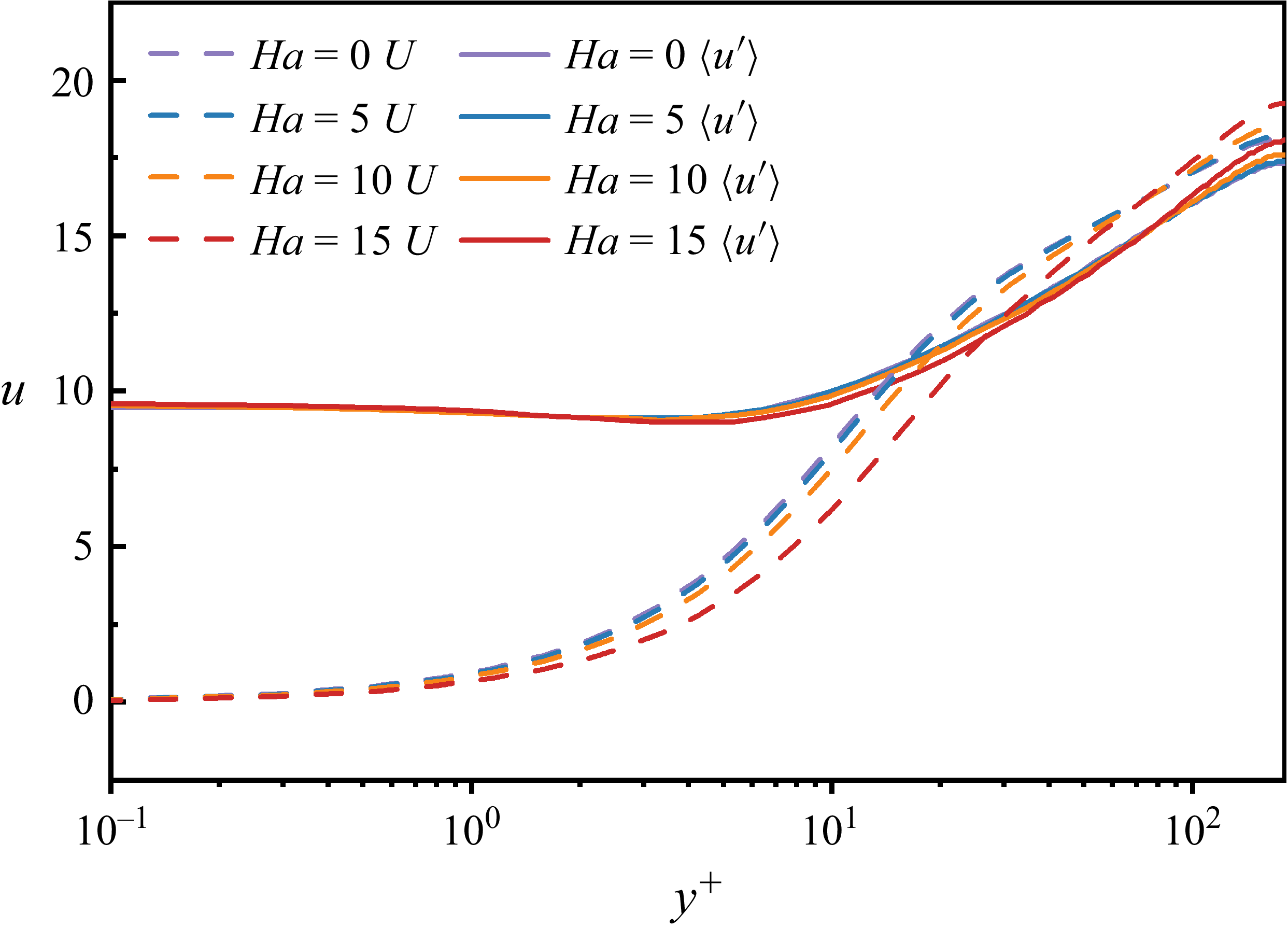
Propagation velocities of different fluctuating variables across the channel. The solid line represents the mean velocity, and the dashed line represents the propagation velocities of the streamwise-fluctuating velocity.

Figure 14 depicts the wall-normal distribution of the convection velocity of velocity fluctuations for different Hartmann numbers. Within the viscous sublayer, the convection velocity is essentially independent of
 $\textit{Ha}$
and markedly exceeds the mean velocity, consistent with classical findings (Kim & Hussain Reference Kim and Hussain1993). In the buffer layer and outer region, it scales approximately with the local mean flow. As the magnetic field intensifies, the mean velocity in the buffer layer decreases and the associated convection velocity correspondingly declines; by contrast, in the outer region the mean velocity increases with
 $\textit{Ha}$
, and the convection velocity of the fluctuations rises appreciably.
3.3.2. Streak density and lifetime
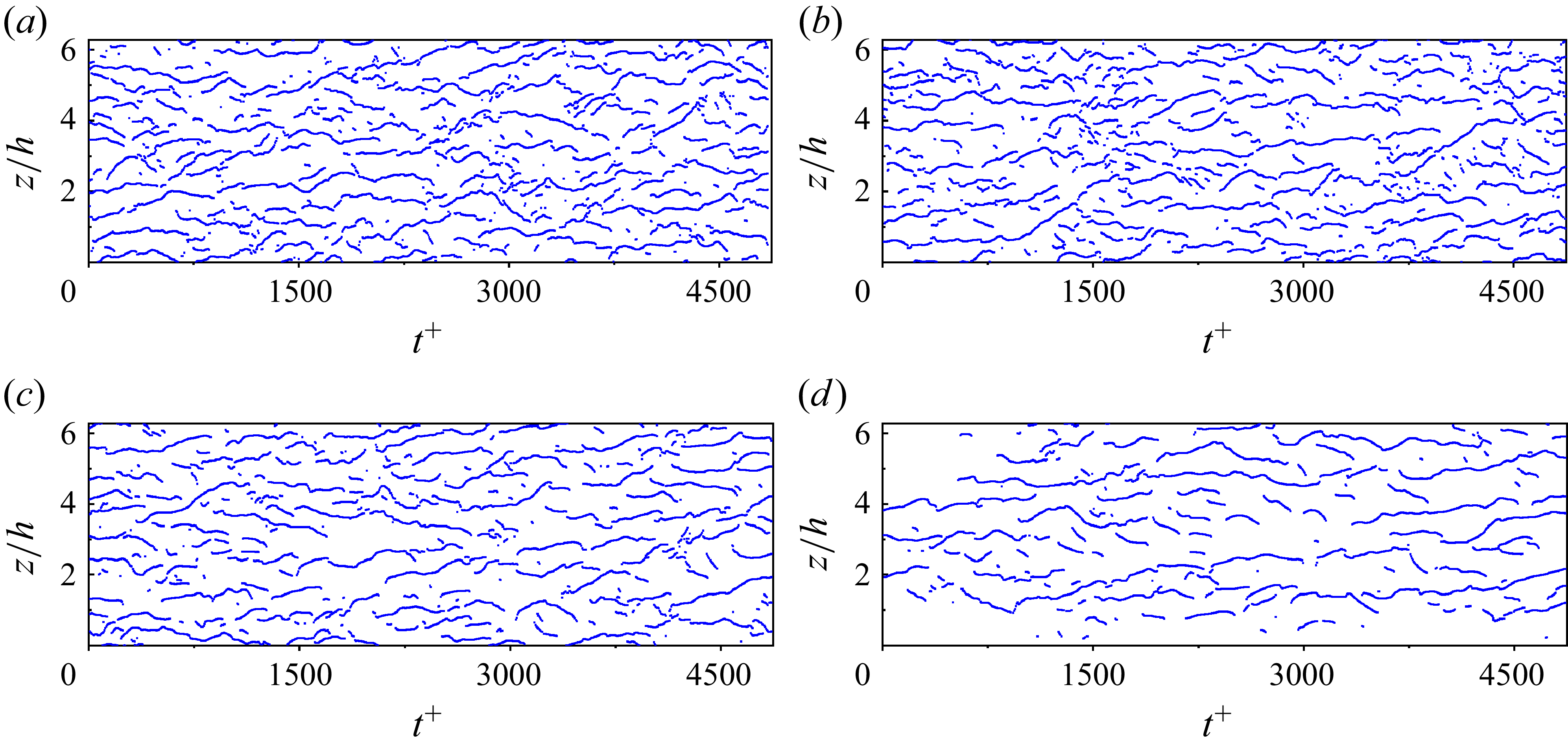
Using these computed advection velocities from figure 14, we conducted a spatiotemporal trajectory analysis of streak structures at
 $y^+ = 14$
at different Hartmann number, shown in figure 15. To ensure sufficient statistical sampling, streaks are tracked from five equally spaced initial streamwise positions (
 $x_{r0}^+ = 200, 200 + L_x^+/5, \ldots$
) across the domain, and the results are aggregated to compute the streak density and lifetime statistics. The lifetime of a streak is recorded as the interval from its first identification to its eventual dissipation. At
 $\textit{Ha}=0$
, the lifetimes of large-scale elongated streaks predominantly range between
 $t^+ \approx 300$
and
 $800$
, with spanwise shifts approximately
 $100$
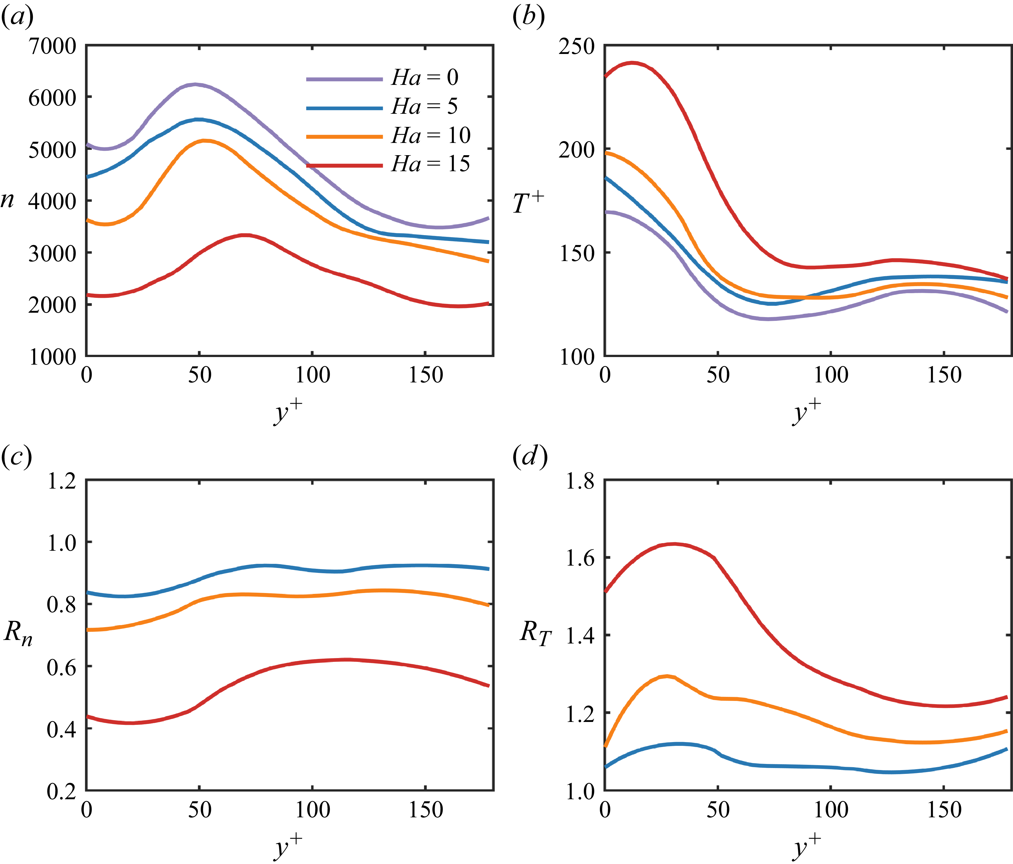
wall units, consistent with prior studies (Jiménez et al. Reference Jiménez, Kawahara, Simens, Nagata and Shiba2005; Flores & Jiméaqnez Reference Flores and Jiméaqnez2010; Abe et al. Reference Abe, Antonia and Toh2018; Zhou et al. Reference Zhou, Xu and Jiménez2022). Notably, long-lived streaks frequently coexist with shorter-lived structures. According to Zhou et al. (Reference Zhou, Xu and Jiménez2022), this is likely due to the interaction (termed ‘gathering’ and ‘scattering’) between outer-region large-scale structures and near-wall low-speed streaks. These shorter-lived streaks are commonly viewed as intermediaries transferring energy towards viscous dissipation scales, despite being larger than actual dissipation scales (owing to the chosen averaging window size). As the magnetic field intensifies, the streak density gradually decreases, while streak lifetimes extend significantly, reaching durations as high as
 $t^+\approxeq 1800$
at
 $\textit{Ha}=15$
. Following Abe et al. (Reference Abe, Antonia and Toh2018), the increase in streak lifetime corresponds to longer streak structures induced by stronger magnetic fields. Moreover, based on Kolesnikov & Tsinober (Reference Kolesnikov and Tsinober1974) and Burattini et al. (Reference Burattini, Zikanov and Knaepen2010), enhanced magnetic fields attenuate turbulence decay in nonlinear stages, suggesting that increased magnetic strength suppresses the decay rates of large-scale streak structures, thereby prolonging their lifetimes. Furthermore, with rising Hartmann numbers, the density of shorter-lived streaks surrounding long-lived streaks notably declines. This phenomenon partly arises because stronger magnetic fields reduce outer-layer influences on the near-wall region, and partly due to the magnetic suppression of downward energy transport.
Figures 16(a) and 16(c), respectively, depict streak densities and their relative ratios compared to the
 $\textit{Ha}=0$
case across different wall-normal positions. Streak density consistently decreases with increasing Hartmann numbers, and the location of peak streak density gradually shifts away from the wall. This spatial shift aligns well with the observed trends in Reynolds stress peaks at different
 $\textit{Ha}$
numbers (see figure 8). Notably, as shown in figure 16(c), while mild magnetic conditions (
 $\textit{Ha}=5$
) yield limited changes in streak density at larger
 $y^+$
, stronger magnetic fields markedly amplify density reduction, especially near the wall. Specifically, at
 $\textit{Ha}=15$
, the streak density ratio drops to approximately
 $0.4$
of its non-magnetic value in the near-wall region (
 $y^+\lt 50$
), whereas it increases slightly to
 $0.6$
in the outer region, confirming that magnetic fields predominantly suppress streak formation closer to the wall.
Time history of the spanwise locations of streaks in a full-sized channel at
 $y^+=14$
for (a)
 $\textit{Ha}=0$
, (b)
 $\textit{Ha}=5$
, (c)
 $\textit{Ha}=10$
and (d)
 $\textit{Ha}=15$
. Locations of the streaks are determined by the condition (3.4)–(3.5). All data are obtained from the
 $16\pi \times 2 \times 2\pi$
domain (
 $1024 \times 128 \times 200$
grid; see table 1).

Distribution of (a) streak density and (b) streak lifetime across the channel under different
 $\textit{Ha}$
. (c) Ratio of streak density and (d) ratio of streak lifetime relative to the
 $\textit{Ha} = 0$
case, as functions of the wall-normal coordinate
 $y^+$
.

Figure 16. Long description
Panel A: A line graph shows the distribution of streak density across the channel under different conditions. The x-axis represents the wall-normal coordinate y+ ranging from 0 to 150. The y-axis represents streak density n ranging from 1000 to 7000. Four lines represent different Ha values: 0, 5, 10, and 15, with distinct colors for each. The lines show varying trends in streak density across the wall-normal coordinate. Panel B: A line graph shows the distribution of streak lifetime across the channel under different conditions. The x-axis represents the wall-normal coordinate y+ ranging from 0 to 150. The y-axis represents streak lifetime T+ ranging from 100 to 250. Four lines represent different Ha values: 0, 5, 10, and 15, with distinct colors for each. The lines show varying trends in streak lifetime across the wall-normal coordinate. Panel C: A line graph shows the ratio of streak density relative to the case as a function of the wall-normal coordinate y+. The x-axis represents the wall-normal coordinate y+ ranging from 0 to 150. The y-axis represents the ratio of streak density Rn ranging from 0.2 to 1.2. Four lines represent different Ha values: 0, 5, 10, and 15, with distinct colors for each. The lines show varying trends in the ratio of streak density across the wall-normal coordinate. Panel D: A line graph shows the ratio of streak lifetime relative to the case as a function of the wall-normal coordinate y+. The x-axis represents the wall-normal coordinate y+ ranging from 0 to 150. The y-axis represents the ratio of streak lifetime RT ranging from 1.0 to 1.8. Four lines represent different Ha values: 0, 5, 10, and 15, with distinct colors for each. The lines show varying trends in the ratio of streak lifetime across the wall-normal coordinate.
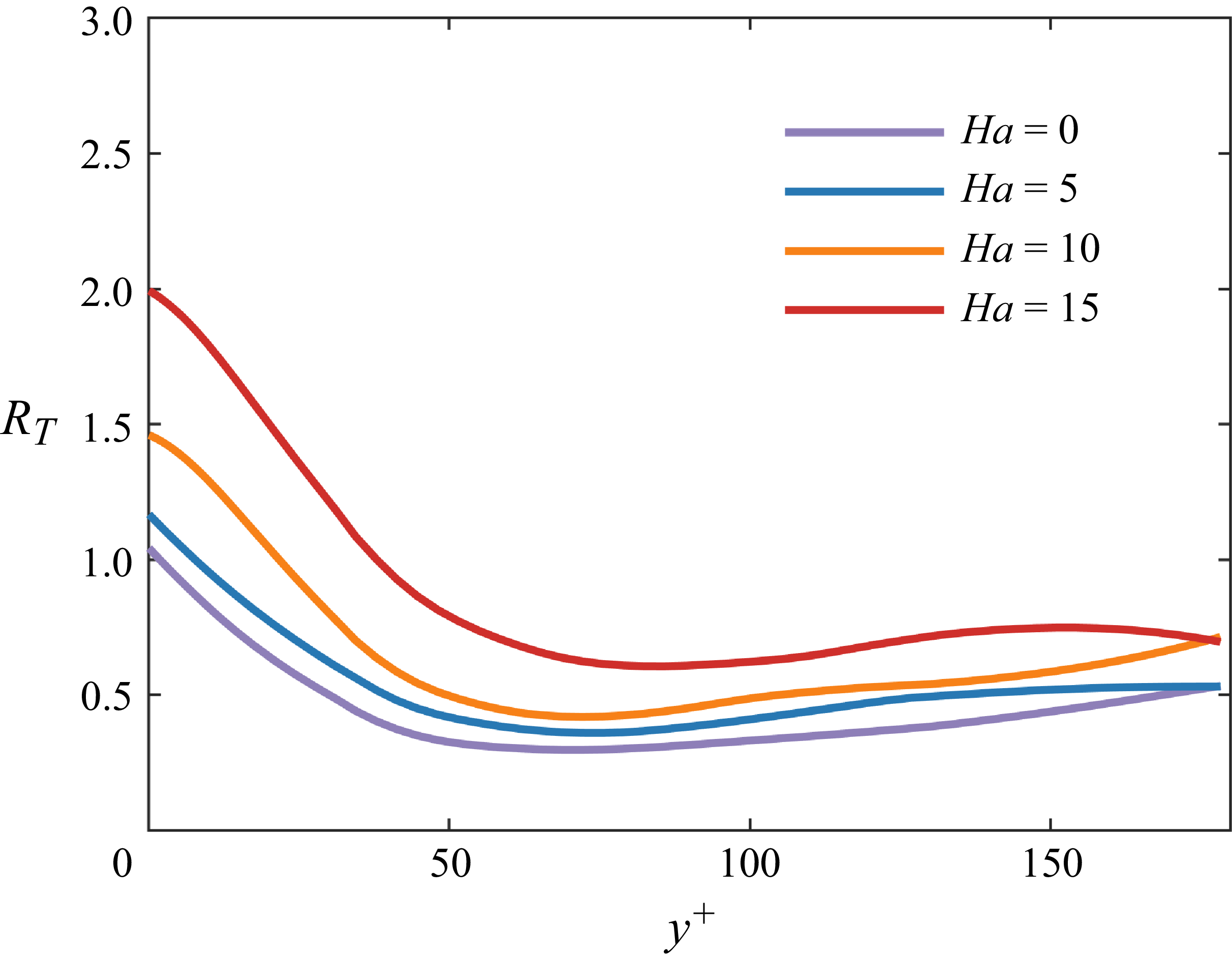
Ratio of the number of streaks with
 $T^+ \gt 30$
to those with
 $T^+ \lt 30$
at different wall-normal locations across the channel.

Figures 16(b) and 16(d) illustrate the variations of streak lifetimes and their ratios relative to the
 $\textit{Ha}=0$
case at different wall-normal positions. The mean streak lifetime is computed as
 $T_{\textit{ave}}^+ = \sum _{i=1}^{Ns} T^+(i)/Ns$
, where
 $Ns$
is the number of streaks. The results indicate that near-wall streak lifetimes decrease gradually with increasing wall-normal distance and eventually stabilise. Moreover, as shown in figure 16(d), stronger magnetic fields significantly increase the near-wall streak lifetimes compared with the outer region.
As previously discussed, streak lifetime is influenced jointly by streak length and magnetic intensity. In the inertial range, the turnover time of eddy structures scales as
 $t_{\textit{turn}}=(l^2/\epsilon )^{1/3}\sim l^{2/3}$
, where
 $l$
is the eddy length and
 $\epsilon$
the turbulent kinetic energy dissipation rate (Pope Reference Pope2001), while Joule dissipation remains uniform across scales (Knaepen & Moreau Reference Knaepen and Moreau2008). Hence, smaller eddies experience stronger inertial dominance; at sufficiently small scales, Joule dissipation is negligible, and isotropic turbulence structures emerge (Klein & Pothérat Reference Klein and Pothérat2010; Pothérat & Klein Reference Pothérat and Klein2014). Motivated by this reasoning, we computed the ratio between the number of longer-lived streaks (
 $t^+\gt 30$
) and shorter-lived streaks (
 $t^+\lt 30$
) across different magnetic intensities (figure 17). Note that the chosen lifetime threshold of
 $t^+=30$
is significantly shorter than typical energy-containing streak lifetimes (
 $t^+\approxeq 800$
), implying minimal magnetic influence at these structures. Results indicate that while streak density across all scales decreases with rising magnetic strength, shorter-lived streaks exhibit a disproportionately larger decline, particularly in the near-wall region. This occurs because stronger magnetic fields suppress downward energy transfer. Additionally, near-wall streaks inherently possess larger length scales than their outer-region counterparts, further amplifying magnetic influences.
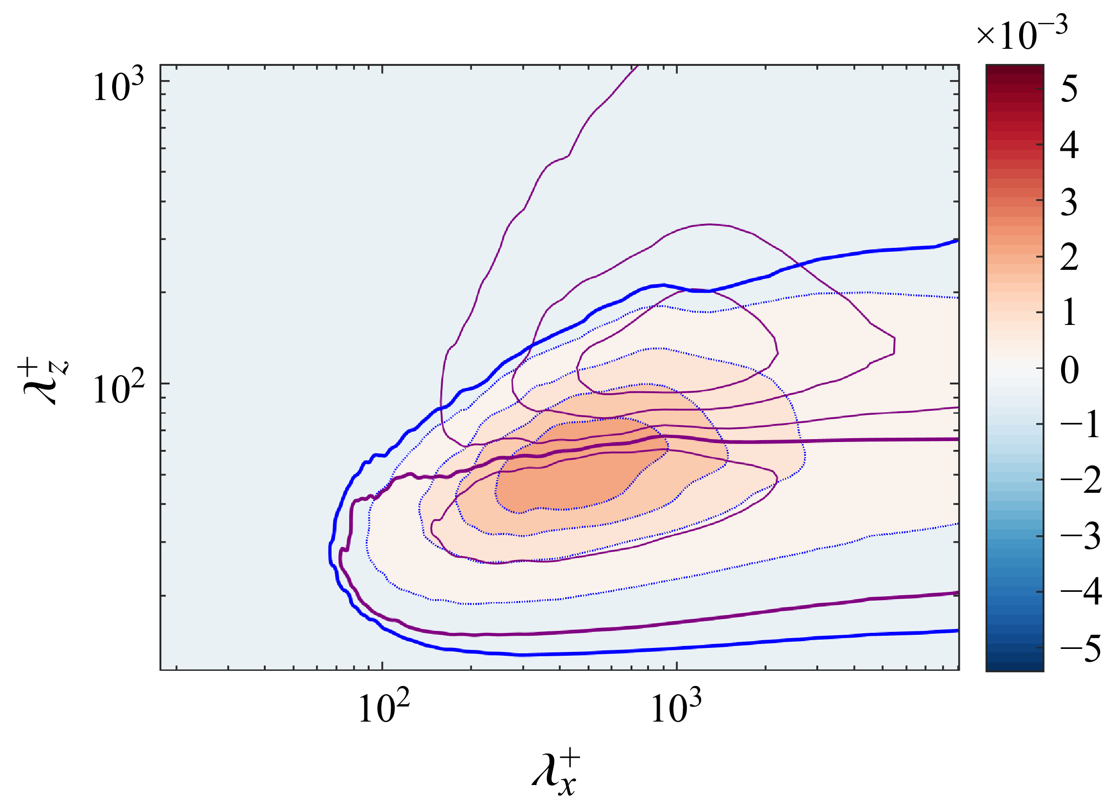
Contours of the two-dimensional spectra of the wall-normal energy flux
 $\tilde {\varTheta }$
at
 $y^+ = 14$
. The colourmap and blue isocontours correspond to
 $\textit{Ha}=0$
, whereas the purple isocontours correspond to
 $\textit{Ha}=15$
; the bold blue and purple curves mark the zero contour.

3.4. Energy budget
To develop a more comprehensive understanding of how magnetic fields influence the wall-normal transport of turbulent energy near the wall, this section focuses on the spectral characteristics of energy fluxes in the wall-normal direction and MHD source. We aim to elucidate how the pathways of energy contributions across turbulent scales evolve under the influence of magnetic fields.
3.4.1. Wall-normal turbulent energy flux
In the absence of a magnetic field (
 $\textit{Ha} = 0$
), the location around
 $y^+ \approx 14$
corresponds to the region of maximum mean shear and serves as the principal site of turbulent kinetic energy production. The generated energy is partly transferred to smaller scales through nonlinear interactions and dissipated via viscosity, while another portion is transported across wall-normal distances, thereby shaping the global energy distribution throughout the channel. To quantitatively describe the scale-dependent characteristics of wall-normal energy transport at different Hartmann numbers, the wall-normal turbulent energy flux is defined as
 \begin{equation} \widetilde {\varTheta }(\boldsymbol{k}, y) = - \int _0^y \widetilde {T} (\boldsymbol{k}, y')\, \mathrm{d}y' .\end{equation}
Figure 18 presents the two-dimensional spectra of wall-normal energy flux
 $\widetilde {\varTheta }$
at
 $y^+ = 14$
. As evident in figure 18, when
 $\lambda _z^+ \gt 100$
, the flux
 $\widetilde {\varTheta } \lt 0$
, indicating that large-scale outer-layer structures are transporting energy towards the near-wall region – a phenomenon commonly interpreted as modulation of the near-wall layer by large-scale structures (Hoyas & Jiménez Reference Hoyas and Jiménez2008; Mizuno Reference Mizuno2016). In contrast, for
 $\lambda _z^+ \lt 100$
, the flux
 $\widetilde {\varTheta } \gt 0$
, signifying energy transport from the near-wall region towards the outer layer, consistent with the conclusions in Mizuno (Reference Mizuno2016). As
 $\textit{Ha}$
increases, the characteristic scales of the dominant structures responsible for both transport directions undergo notable shifts: the streamwise length scales
 $\lambda _x$
increase significantly, which can be attributed to the streamwise stretching effect of the magnetic field and the outward migration of the turbulent kinetic energy peak as discussed above. Meanwhile, the spanwise scales
 $\lambda _z$
of these structures decrease at this wall-normal location, owing to the weakening modulation of the near-wall region by outer-layer large-scale structures under stronger magnetic fields.
Contours of the premultiplied one-dimensional spectra of (a)
 $k_z \sum _{k_x} \widetilde {\varTheta }$
, rendered as functions of the spanwise wavelength
 $\lambda _z$
and the wall-normal distance
 $y$
, and (b) the corresponding premultiplied one-dimensional spectra of
 $k_x \sum _{k_z} \widetilde {\varTheta }$
, presented as functions of the streamwise wavelength
 $\lambda _x$
and the wall-normal distance
 $y$
. The colourmap and the blue isocontours pertain to
 $\textit{Ha}=0$
, while the purple isocontours correspond to
 $\textit{Ha}=15$
; the bold blue and purple curves delineate the zero contour.

To further illustrate the spatial distribution of energy transport, figure 19 shows one-dimensional premultiplied spectra
 $k_z \sum _{k_x}\widetilde {\varTheta }$
and
 $k_x \sum _{k_z} \widetilde {\varTheta }$
, plotted as functions of spanwise wavelength
 $\lambda _z$
, streamwise wavelength
 $\lambda _x$
and wall-normal distance
 $y$
. As shown in figure 19(a), energy transported downward ceases in the viscous sublayer – terminating around
 $y^+ \approx 2$
at
 $\textit{Ha}=0$
and shifting to
 $y^+ \approx 5$
at
 $\textit{Ha}=15$
. This trend implies that as
 $\textit{Ha}$
increases, the ability of logarithmic-layer structures to modulate near-wall turbulence weakens. The viscous sublayer, once responsible for significant energy dissipation, now plays a diminished role as more energy is dissipated via Joule heating during transport, consistent with observations on streak density reduction in § 3.3.2. It is also noteworthy that the spectral peaks of
 $\widetilde {\varTheta }$
exhibit two clear trends with increasing magnetic field: first, a migration away from the wall; and second, a shift towards larger spanwise wavelengths
 $\lambda _z$
. This indicates not only an alteration in the vertical transport path of energy but also a transition of dominant energy-carrying structures towards broader scales, further reinforcing the conclusion that magnetic fields fundamentally reshape multiscale turbulent dynamics.
3.4.2. Magnetohydrodynamic effects on energy budget
In MHD turbulence, energy transport mechanisms are profoundly affected by the Lorentz forces introduced by the magnetic field. In the inner layer – particularly beyond
 $ y^+ \gt 20$
– the generation and redistribution of turbulent kinetic energy are governed primarily by three mechanisms: the production term, nonlinear transport and dissipation through both viscosity and Joule dissipation. As discussed in § 3.2.1, we examined the impact of Reynolds stress on turbulent kinetic energy. Subsequently, we will primarily examine the influence of MHD source terms on energy transport under varying Hartmann numbers.
Premultiplied spectra of MHD source term
 $k_x \sum _{k_z} \tilde {S_1}$
as a function of
 $\lambda _x^+$
and
 $y^+$
for: (a)
 $\textit{Ha}=5$
, (b)
 $\textit{Ha}=10$
and (c)
 $\textit{Ha}=15$
.

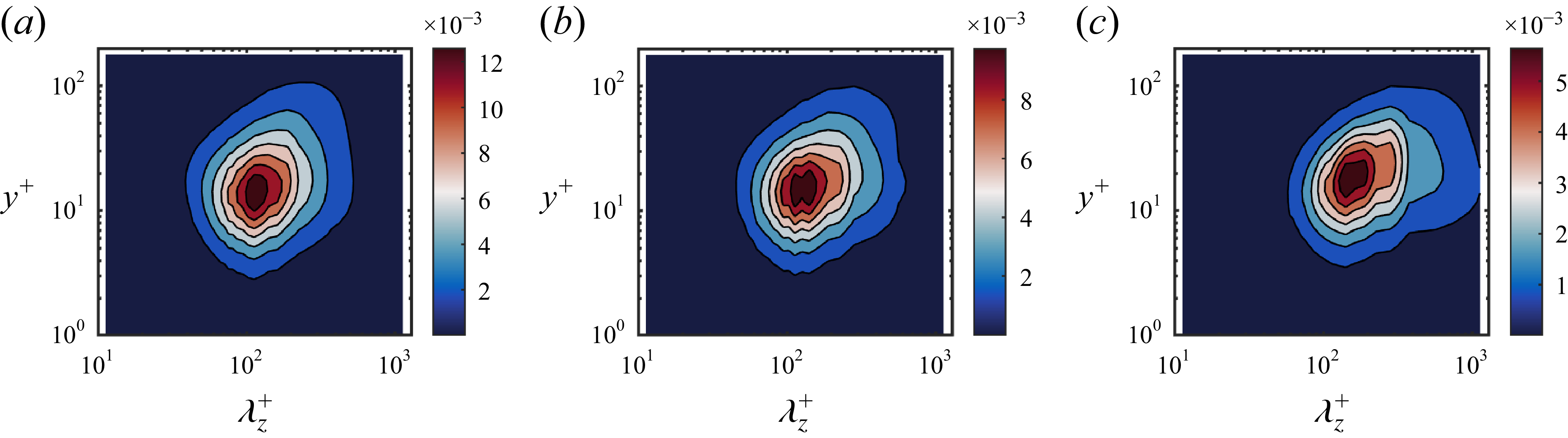
Premultiplied spectra of MHD source term
 $k_z \sum _{k_x} \tilde {S_1}$
as a function of
 $\lambda _z^+$
and
 $y^+$
for: (a)
 $\textit{Ha}=5$
, (b)
 $\textit{Ha}=10$
and (c)
 $\textit{Ha}=15$
.

The magnetic influence on flow comprises both source and dissipation terms. The dissipation term, proportional to
 $\sigma B^2(u^2 + v^2)$
, scales directly with turbulent kinetic energy. While Lorentz forces are generally expected to stretch vortical structures in the direction of the magnetic field, our results reveal an intriguing asymmetry: magnetic effects lead to significantly more stretching in the streamwise direction than in the spanwise direction for near-wall coherent structures, as shown in figure 20. To investigate this further, figure 21 presents the premultiplied spectrum
 $k_z \sum _{k_x} \tilde {S_1}$
, representing one of the key magnetic source terms which represents the correlation between wall-normal electric potential gradient and streamwise velocity fluctuation. It is evident that the energy injection peak of
 $\tilde {S_1}$
shifts to larger scales and migrates away from the wall with increasing magnetic strength. This trend is strongly correlated with the observed streamwise elongation of streaks as
 $\textit{Ha}$
increases, suggesting that the growth of near-wall coherent structures in the streamwise direction is largely driven by the
 $\tilde {S_1}$
term. While
 $\tilde {S_1}$
supplies energy needed for structural elongation, the same scales are subject to intense Joule dissipation, resulting in a competition between energy injection and dissipation. Consequently, structures expand morphologically but remain energetically constrained.
Premultiplied spectra of MHD source term
 $k_x \sum _{k_z} \tilde {S_2}$
as a function of
 $\lambda _x^+$
and
 $y^+$
for: (a)
 $\textit{Ha}=5$
, (b)
 $\textit{Ha}=10$
and (c)
 $\textit{Ha}=15$
.

On the other hand, figures 22 and 23 depict the premultiplied spectra
 $k_x \sum _{k_z} \tilde {S_2}$
and
 $k_z \sum _{k_x} \tilde {S_2}$
, revealing another class of magnetic source terms. Compared with
 $\tilde {S_1}$
,
 $\tilde {S_2}$
is markedly weaker and predominantly concentrated in the outer layer. Its peak shifts farther from the wall with increasing
 $\textit{Ha}$
, and the associated spanwise wavelength
 $\lambda _z$
also increases, indicating that in the outer region, magnetic regulation of turbulence manifests more strongly in the spanwise direction. This contrasts with the near-wall dynamics, where streamwise elongation dominates, and illustrates the spatially selective nature of magnetic control across different structural scales.
Premultiplied spectra of MHD source term
 $k_z \sum _{k_x} \tilde {S_2}$
as a function of
 $\lambda _z^+$
and
 $y^+$
for: (a)
 $\textit{Ha}=5$
, (b)
 $\textit{Ha}=10$
and (c)
 $\textit{Ha}=15$
.

In summary, magnetic fields drive the streamwise growth of near-wall coherent structures through the source term
 $\tilde {S_1}$
while simultaneously imposing strong suppression across all scales via Joule dissipation. This interaction yields an evolution pathway characterised by structural elongation yet limited energetic growth. Meanwhile, although the outer-layer source term
 $\tilde {S_2}$
is weaker, its spanwise scale expansion suggests that attached vortices broaden in the spanwise direction under stronger magnetic fields. These findings collectively demonstrate that the spatial distribution and scale-dependent characteristics of energy sources and dissipation in MHD turbulence dictate the evolutionary fate of turbulent structures subjected to magnetic fields.
4. Summary and conclusions
This study investigates the influence of a spanwise magnetic field on low-Reynolds-number channel flow (
 $\textit{Re}_{\tau }=180$
), revealing the magnetic field’s pivotal role in energy distribution, streak dynamics and energy transport. Notably, at
 $\textit{Ha}=15$
and
 $y/h\gt 0.3$
, the streamwise velocity fluctuations intensify, surpassing the no-field level. Spectral analysis suggests that this surge arises from the emergence of outer-layer large-scale structures. Premultiplied streamwise turbulent kinetic energy spectra further show that, with increasing Hartmann number
 $\textit{Ha}$
, the near-wall streaks elongate markedly in the streamwise direction: the characteristic length grows from
 $\lambda _x^+\approx 1000$
at
 $\textit{Ha}=0$
to
 $\lambda _x^+\approx 1800$
at
 $\textit{Ha}=15$
, while the peak shifts outward from
 $y^+\approx 14$
to
 $y^+\approx 22$
. At
 $\textit{Ha}\approx 15$
, a bimodal structure appears, with a second peak near
 $\lambda _x^+\approx 3000$
, indicating a new dynamical regime. Meanwhile, the spanwise scale increases from
 $\lambda _z^+\approx 100$
to
 $\lambda _z^+\approx 130$
, though far less dramatically than the streamwise extension. Scale-integrated turbulent kinetic energy shows that the near-wall large-scale energy fraction rises sharply with field strength (for
 $k_x\lt 10$
, from
 $68\,\%$
to
 $85\,\%$
), and the outer layer also experiences an increase in large-scale energy – trends primarily attributable to magnetic suppression of downscale energy transfer.
Further analysis links the near-wall bimodality to the alternating dominance of high- and low-momentum regions. The high-momentum state comprises alternating high- and low-speed streaks of scale
 $\lambda _x^+\approx 1000$
(the short-scale peak), whereas the low-momentum state is governed by low-speed streaks with
 $\lambda _x\approx 20h$
(the long-scale peak). Numerically, the streak density and intensity in low-momentum regions are consistently lower than in their high-momentum counterparts. Cross-correlation-based convection-velocity statistics reveal that, in the viscous sublayer, convection velocities are insensitive to
 $\textit{Ha}$
and exceed the mean velocity; in the buffer and outer layers, they scale with the local mean. Streak statistics further show that, as
 $\textit{Ha}$
increases, streak density declines while lifetimes lengthen markedly: near-wall lifetimes cluster around
 $t^+\approx 300{-}800$
at
 $\textit{Ha}=0$
but reach
 $t^+\approx 1800$
at
 $\textit{Ha}=15$
. Simultaneously, the peak location migrates away from the wall and the fraction of small scales diminishes, indicating that the magnetic field both suppresses decay (thereby prolonging persistence) and weakens near-wall energy replenishment, allowing more turbulent energy to be removed by Joule dissipation.
Energy-budget diagnostics underscore the magnetic field’s far-reaching impact on transport mechanisms. With increasing
 $\textit{Ha}$
, modulation of the near-wall region by outer-layer large scales weakens; the dominant carriers of wall-normal energy transport shift towards larger scales and migrate away from the wall. The Lorentz-force source terms –
 $\tilde {S_1}$
and
 $\tilde {S_2}$
– exhibit pronounced scale dependence in the near-wall and outer layers, respectively:
 $\tilde {S_1}$
drives the streamwise elongation of near-wall coherent structures, whereas
 $\tilde {S_2}$
fosters spanwise expansion of outer-layer structures, with the former far outweighing the latter in dynamical significance.
Several open questions emerge from the present findings. The most immediate concerns the very large-scale structures that appear in the outer layer at
 $\textit{Ha}=15$
– whether they survive at higher
 $\textit{Re}_\tau$
, how they are sustained and whether they couple back to the near-wall cycle, all remain unknown. More broadly, the present spectral analysis captures only the wall-parallel scales; a full picture of energy transfer requires resolving the wall-normal direction as well. The Karman–Howarth–Monin–Hill framework (Hill Reference Hill2002; Marati et al. Reference Marati, Casciola and Piva2004; Cimarelli et al. Reference Cimarelli, De Angelis, Jiménez and Casciola2016), which tracks energy exchange simultaneously across scales and in physical space, is well suited to this task.
Acknowledgements
The authors greatly appreciate the anonymous reviewers for their constructive comments, which significantly helped improve the manuscript.
Funding
This work was supported by the National Natural Science Foundation of China (NSFC) under Grant Nos. 52522605 and U24A6007, and by the Chinese Academy of Sciences (CAS) under Grant Nos. YSBR-087 and XDB0790103.
Declaration of interests
The authors report no conflict of interest.

 Lx
 Lz
 h
 Δx
 Δz
 Δymin
 Δymax
 Nx
 Ny
 Nz
 Δt+
 Nf
 Ubulk+
 Reτ=180
 Ha
 16π×2×2π
 4π×2×2π
 uτ

 ⟨u′u′⟩1/2
 ⟨v′v′⟩1/2
 ⟨w′w′⟩1/2
 ⟨u′v′⟩
 Ha
 16π×2×2π
 4π×2×2π
 uτ

 kxΣkzϕuu/uτ2
 λx+
 y+
 Ha=0
 Ha=5
 Ha=10
 Ha=15
 kxΣkzϕuu/uτ2
 λx+
 y+
 Ha=15
 Lx×Ly×Lz=64π×2×2π

 kzΣkxϕuu/uτ2
 λz+
 y+
 Ha=0
 Ha=15

 kxΣkzϕuv/uτ2
 λx+
 y+
 Ha=0
 Ha=5
 Ha=10
 Ha=15
 kx<10
 kz<10
 (δu′)3(r)
 r
 y+≈140
 Ha=15
 Lx×Ly×Lz=64π×2×2π
 Nf=200

 u′
 y+=20
 Ha=15

 Ha=0
 Ha=5
 Ha=10
 Ha=15

 q
 Ha=15
 y+=14
 Ha=0
 Ha=5
 Ha=10
 Ha=15
 16π×2×2π
 1024×128×200
 Ha
 Ha=0
 y+
 T+>30
 T+<30
 Θ~
 y+=14
 Ha=0
 Ha=15

 kz∑kxΘ~
 λz
 y
 kx∑kzΘ~
 λx
 y
 Ha=0
 Ha=15

 kx∑kzS1~
 λx+
 y+
 Ha=5
 Ha=10
 Ha=15
 kz∑kxS1~
 λz+
 y+
 Ha=5
 Ha=10
 Ha=15
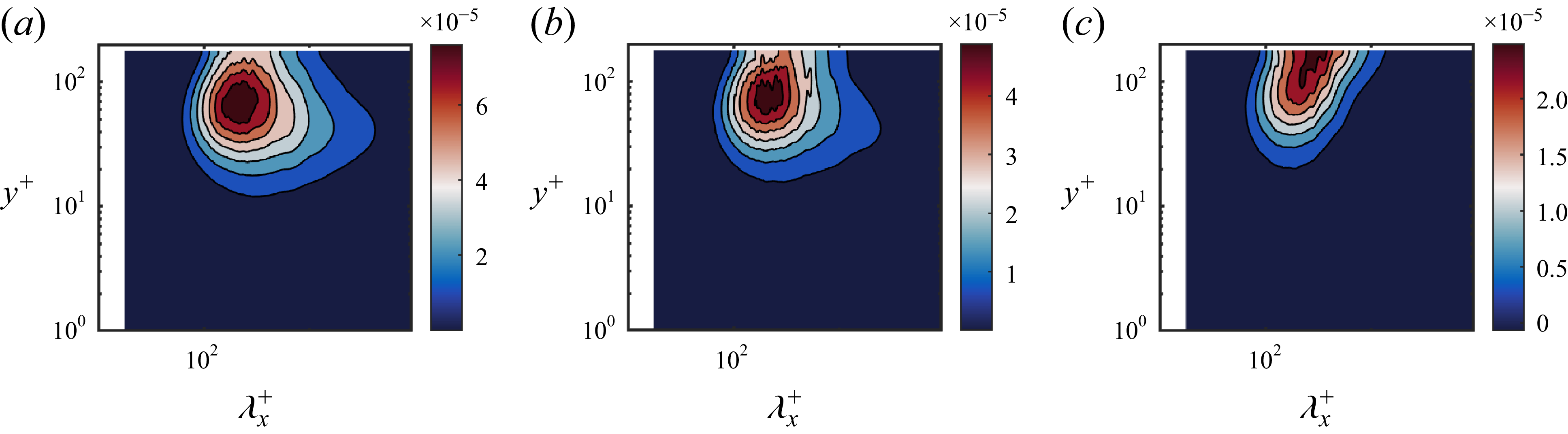
 kx∑kzS2~
 λx+
 y+
 Ha=5
 Ha=10
 Ha=15
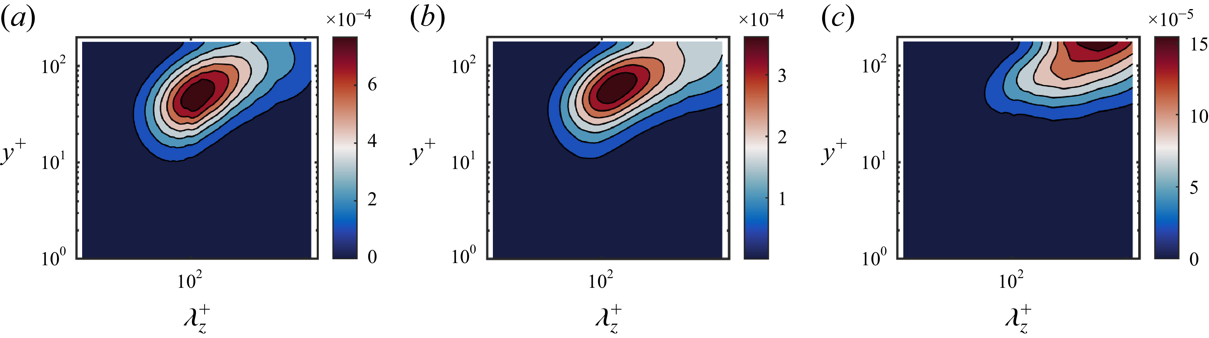
 kz∑kxS2~
 λz+
 y+
 Ha=5
 Ha=10
 Ha=15


