NOMENCLATURE
- β
-
side sliding angle
- B
-
airship buoyancy
- cϕ, c ψ
-
roll angle gain and yaw rate gain for the high-level controller
- Cyi, Cz
-
aerodynamic force coefficient along y-axis and z-axis(i = 1,2,3)
- Cl , Cm , Cn
-
aerodynamic moment coefficients along x-, y-, and z-axis
- dx , dz
-
distances from the CV to the propeller in the x- and z-axis
- e
-
trajectory tracking error vector
- F b , F g , F w
-
the body fixed frame (centred at the CV), the Earth reference frame, the wind-axes frame
- F A , F CP , F d , F GB
-
airship aerodynamic forces vector, sum of centrifugal and Coriolis vector forces, sum of gravity and buoyancy vector, sum of control and propulsive vector
- f A i , f CP i , f d i , f GB i
-
forces of F A , F CP , F d , F GB along i axis (i = x, y, z)
- G
-
airship gravity
- I x,I y,I z
-
airship moments of inertia along x-, y-,and z-axis
- I xy,I yz,I xz
-
airship products of inertia
- Ixa , Iya , Iza , Ixza
-
apparent moments of inertia or product of inertia
-
 $\bm{J} \in {\mathbb{R}^{3 \times 3}}$
-
airship inertia matrix
- Ji
-
sum of apparent moments of inertia and moments of inertia with Ji = Ii+Iia (i = x, y, z, xz)
- k 1, k 2, k 3
-
ellipsoid inertia factors
- K 1, K 2, K 3
-
controller parameters of the vectorial backstepping method
- K P, K D
-
control gains of proportion and differentiation
- m
-
total mass of the airship
- m 1, m 2, m 3
-
airship apparent masses
- m x, m y, m z
-
sum of airship apparent masses and masses m
-
${\bm{M}_a} \in {\mathbb{R}^{6 \times 6}}$
-
generalised apparent mass
- n A i, n CP i, n d i, n GB i
-
moments resulted by F A , F CP , F d , F GB (i = x, y, z)
- p
-
optimal perturbation
-
$\bar{q}$
-
dynamic pressure
-
$\bm{R} \in {\mathbb{R}^{3 \times 3}}$
-
direction cosine matrix
- Tp , Ts
-
thrusts of the port side and the starboard side
- T
-
sample period or motion period
- umin , umax
-
lower and upper bounds of the actuator position
-
${\bm{\dot{u}}_{\min }}$
,
${\bm{\dot{u}}_{\max }}$
-
lower and upper bounds of the actuator rotating rate
- Vi
-
control Lyapunov function (i = 1, 2, 3, l, h)
- τ
-
actuator time delay
-
$\bm{\upsilon }$
,
${\bm{\upsilon }_d}$
-
airship practical and desired translational velocity vector (u, v,w)T in F b
-
${\bm{\upsilon }_c}$
,
${\bm{\upsilon }_r}$
-
airship commanded and referenced translational velocity vector in F g
-
V
= (
$\bm{\upsilon }$
,
ω
)T
-
the generalised velocity in F b
- W u , W v
-
weight matrices of virtual control and actuator
- xG , zG
-
coordinate position of CG alone x- and z-axis
- z i
-
virtual state in the controller design (i = 1,2,3,4)
- δeL , δeR
-
left and right elevator deflection
- δrU , δrB
-
upper and bottom rudder deflection
- μ
-
tilt angle of the propellers
- η , ηd , ηr
-
practical attitude vector, desired and referenced attitude vectors
- η lgr, λlgr
-
the Lagrange multipliers associated with constraints of equality and inequality
- ξ , ξ d
-
practical and desired position vectors (x, y, z)T in F g
- ρ
-
density of the ambient air
- φ, θ, ψ
-
airship Euler angles: roll, pitch, yaw
- ω
-
airship angular rate vector (p, q, r)T
-
$\bm{\dot{\Omega }}$
-
desired acceleration vector or control law
- σ 1, σ 2
-
design parameters representing the stiffness and damping coefficients
- ∇
-
volume of the airship hull


Subscripts
- d
-
desired input values to the controller (e.g., desired trajectory and speed)
1.0 INTRODUCTION
Stratospheric airships are generally designed to be under-actuated for weight and efficiency considerations. Unlike fully actuated systems, it is quite challenging to control under-actuated systems because at least one degree of freedom cannot be directly controlled with independent control input. Moreover, airship dynamics are inherently non-linear and distinct from common aircraft dynamics. The Centre of Gravity (CG) of an airship is usually below the Centre of Volume (CV). And the apparent mass and inertia of the airship cannot be ignored. These characteristics make the flight control design for the stratospheric airship rather complicated. Therefore, traditional control design approaches(Reference Kulczycki, Joshi and Hess1–Reference Benjovengo, Paiva and Bueno3) using the linearised model at the trimming points are hard to accomplish, because they are only valid in a small neighbourhood of the equilibrium state, and control performances of these approaches are degraded as operating conditions change intensively.
To overcome the theoretical limitations of linear control methods, many non-linear control approaches have been studied for airship dynamics. Wang et al. designed a non-linear controller based on a differential geometric method to solve attitude tracking problem of a small airship(Reference Wang and Shan4). Acosta proposed a dynamic inversion method to control an autonomous airship(Reference Acosta and Joshi5). The advantages of these non-linear methods are that non-linearities are completely cancelled out, and then linear control methods can be applied to the feedback linearised system. The main drawback of these approaches is that accurate models are necessary for design. When the model error exists, the robustness cannot be guaranteed.
Compared with the above methods, the backstepping approach is systematic and flexible, which can be used to design a robust controller for strict feedback systems through construction of Control Lyapunov Functions (CLFs). Non-linear backstepping techniques(Reference Krstic, Kanellakopoulos and Kokotovic6) have been widely studied for different control research objects such as fighter aircrafts(Reference Sonneveldt, Van Oort and Chu7), transport aircrafts(Reference Zhang, Chen and Wei8) and marine vehicles(Reference Fossen9). The backstepping method was first used to deal with the control problem of a decomposed airship model(Reference Hygounenc and Soueres10). Azinheira proposed backstepping control designs for hover stabilisation and path-tracking of a 6 degree-of-freedom (6-DOF) non-linear airship model(Reference Azinheira, Moutinho and De Paiva11,Reference Azinheira, Moutinho and de Paiva12) . Lee developed a vectorial backstepping controller for a 50 m mid-altitude unmanned airship(Reference Lee, Lee and Won13). And a fuzzy adaptive backstepping approach was presented for hovering control of a stratospheric airship in Reference Yang, Wu and ZhengRef. 14. However, all the above backstepping designs are focused on fully actuated airship models, which cannot guarantee the performance for the under-actuated cases.
Therefore, the under-actuated airship control problem has been an active topic recently. Trajectory tracking, path following and hover stabilisation controllers have been developed for the under-actuated vehicles via robust gain scheduling(Reference Moutinho, Moutinho, de Paiva and Bueno15), trajectory linearisation control method(Reference Zheng, Huo and Wu16,Reference Liu, Lu and Jing17) and different kinds of backstepping approaches(Reference Repoulias and Papadopoulos18,Reference Zheng and Wu19) . Recently Daskiran proposed a control without model information by using expert demonstrations and reinforcement learning method(Reference Daskiran and Dogan20). However, most non-linear airship control studies only regard forces and moments as control inputs without control allocation, which are uneasy to realize in practical engineering.
With control allocation, Liesk(Reference Liesk, Nahon and Boulet21) proposed a waypoint tracking controller for an unmanned finless airship. However, according to Reference HarkegardRef. 22, the quadratic optimisation algorithm in Reference Liesk, Nahon and BouletRef. 21 is inefficient in computation. Motivated by the work of Liesk(Reference Liesk, Nahon and Boulet21,Reference Liesk, Nahon and Boulet23) , in this paper, a novel Vectorial Backstepping Trajectory Tracking Controller (VBTTC) is proposed for an under-actuated stratospheric airship. The VBTTC has a two-level control structure including a low-level controller and a high-level controller. The low-level controller can be regarded as an autopilot with a stability augmentation system to stabilise airship's attitude and velocity. And the high-level controller can be considered as a guidance control to generate airship position commands.
In summary, the main contributions of this paper are the following:
-
• The non-linear dynamics system of the unmanned stratospheric airship is stabilised by using backstepping control.
-
• The trajectory tracking problem in three-dimensional (3D) space for a full 6-DOF non-linear airship is solved by the proposed VBTTC method. The VBTTC has a two-level control structure including a low-level controller to stabilise attitude and velocity and a high-level controller to generate airship desired commands.
-
• A backstepping control is applied directly the rigid body dynamics expressed on vector form. And the novel low-level controller is designed by vectorial backstepping method for the under-actuated non-linear airship.
-
• An active-set–based control allocation is incorporated into the low-level controller to optimise control surface deflections and thrust forces for the unmanned airship.
This paper is organised as follows. The non-linear model of the under-actuated stratospheric airship and trajectory tracking problem are presented in Section 2. A novel VBTTC is proposed in Section 3, and stability is analysed for the associated closed-loop tracking error system. Simulations of two under-actuated cases are demonstrated the VBTTC performances in Section 4. Section 5 gives some conclusions.
2.0 PROBLEM FORMULATION
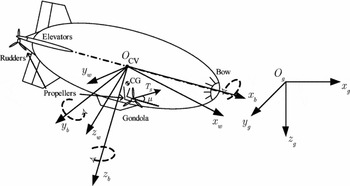
The stratospheric airship studied in this paper is shown as Fig. 1. The control surfaces of the airship are two rudders and two elevators in the tail fins. Two vectored propellers are equipped on both sides of the hull, and another one is on the stern for hovering control. The gondola below the airship envelope is equipped with control system and other devices. Some assumptions related to airship dynamics are listed as follows:
-
1) The effects of Earth curvature are not taken into account.
-
2) The pressure inside the envelope is high enough to maintain the airship as a rigid body.
-
3) The CG lies on the symmetry plane below the CV, see Fig. 1.
-
4) The atmospheric parameters are stable, and disturbances are bounded.
-
5) Actuators dynamics, propellers dynamics and sensors noise are ignored.
Coordinate frames and structure of the stratospheric airship.

2.1 Kinematics model
The kinematic equations of position and attitude are(Reference Moutinho, Moutinho, de Paiva and Bueno15,Reference Zheng, Huo and Wu16)
 $$\begin{equation}
\left\{ \arraycolsep5pt\begin{array}{@{}l@{}} \dot{\xi } = \bm{R}\left( \eta \right)\upsilon \\ \dot{\eta } = \bm{J}(\eta )\omega \end{array} \right.
\end{equation}$$
The direction cosine matrix is
 $$\begin{equation}
\bm{R}\left( \eta \right) = \left( {\arraycolsep5pt\begin{array}{@{}*{3}{c}@{}} {c\theta c\psi }&{ - c\phi s\psi + s\phi s\theta c\psi }&{s\psi s\phi + c\phi s\theta c\psi }\\ {c\theta s\psi }&{c\phi c\psi + s\phi s\theta s\psi }&{ - s\phi c\psi + c\phi s\theta s\psi }\\ { - s\theta }&{s\phi c\theta }&{c\theta c\phi } \end{array}} \right),
\end{equation}$$
where s and c denote sine and cosine functions, respectively. And the matrix J is
 $$\begin{equation*}
\bm{J}(\eta ) = \left( {\arraycolsep5pt\begin{array}{@{}*{3}{c}@{}} 1&{s\phi \tan \theta }&{c\phi \tan \theta }\\ 0&{c\phi }&{ - s\phi }\\ 0&{s\phi \sec \theta }&{c\phi \sec \theta } \end{array}} \right),
\end{equation*}$$
where |θ| < π/2 is assumed to avoid the singularity of matrix because θ = ±π/2 is not likely to be encountered during practical operations of airship.
2.2 Dynamics model
Airship dynamics are given as follows(Reference Mueller, Paluszek and Zhao24–Reference Gates27):
 $$\begin{equation}
{\bm{M}_a}\bm{\skew4\dot{V}} = {\bm{F}_d} + {\bm{F}_{GB}} + {\bm{F}_A} + {\bm{F}_{CP}}
\end{equation}$$
Airship forces and moments on the right-hand side of Equation (3) can be expressed as in Reference Mueller, Paluszek and ZhaoRefs 24–Reference Gomes26. The generalised mass matrix is
 $$\begin{equation*}
{\bm{M}_a} = \left[{\arraycolsep5pt\begin{array}{@{\hskip-5pt}*{7}{c}@{}}
&{{m_x}}&0&0&0&{m \cdot {z_G}}&0\\
*& * &{{m_y}}&0&{ - m \cdot {z_G}}&0&{m \cdot {x_G}}\\
*& *&*&{{m_z}}&0&{ - m \cdot {x_G}}&0\\
*& *&*&*&{{J_x}}&0&{ - {J_{xz}}}\\
*& *&*&*&*&{{J_y}}&0\\
*& *&*&*&*&*&{{J_z}} \end{array}} \right],
\end{equation*}$$
where * denotes the symmetrical elements of the matrix. The sum force of gravity and buoyancy can be described as
 $$\begin{equation*}
{\bm{F}_{GB}} = \left[ {\arraycolsep5pt\begin{array}{@{}*{1}{c}@{}} {{f_{GBx}}}\\ {{f_{GBy}}}\\ {{f_{GBz}}}\\ {{n_{GBx}}}\\ {{n_{GBy}}}\\ {{n_{GBz}}} \end{array}} \right] = \left[ {\arraycolsep5pt\begin{array}{@{}*{1}{c}@{}} { - \left( {G - B} \right)\sin \theta }\\ {\left( {G - B} \right)\cos \theta \sin \phi }\\ {\left( {G - B} \right)\cos \theta \cos \phi }\\ {G\left( {{z_G}\cos \theta \sin \phi } \right)}\\ { - G\left( {{z_G}\sin \theta + {x_G}\cos \theta \cos \phi } \right)}\\ {G\left( {{x_G}\cos \theta \sin \phi } \right)} \end{array}} \right]
\end{equation*}$$
The thrust force on the stern is not considered in flight, which is mainly used for hovering. For simplicity, two tilt angles and thrust forces of the thrusters are assumed to be equal, and the effect of rudders on the side force is also ignored. The control force equations are
 $$\begin{equation}
{\bm{F}_{CP}} = \bm{B}u,
\end{equation}$$
that is,
 $$\begin{equation}
\left[ {\arraycolsep5pt\begin{array}{@{}*{1}{c}@{}} {{f_{CPx}}}\\ {{f_{CPz}}}\\ {{n_{CPx}}}\\ {{n_{CPy}}}\\ {{n_{CPz}}} \end{array}} \right] = \left[ {\arraycolsep5pt\begin{array}{@{}*{6}{c}@{}} 1&0&0&0&0&0\\ 0&1&{\bar{q}{C_z}}&{\bar{q}{C_z}}&0&0\\ 0&0&{\bar{q}{C_l}}&{ - \bar{q}{C_l}}&{\bar{q}{C_l}}&{ - \bar{q}{C_l}}\\ {d_z}&{d_x}&{\bar{q}{C_m}}&{\bar{q}{C_m}}&0&0\\ 0&0&0&0&{\bar{q}{C_n}}&{\bar{q}{C_n}} \end{array}} \right]\left[ {\arraycolsep5pt\begin{array}{@{}*{1}{c}@{}} {{T_x}}\\ {{T_z}}\\ {{\delta _{eL}}}\\ {{\delta _{eR}}}\\ {{\delta _{rU}}}\\ {{\delta _{rB}}} \end{array}} \right],
\end{equation}$$
where B is the control effectiveness matrix, u represents thrust forces and control surface deflections. TX and TZ are thrust components in x axis and z axis, respectively. The thrust forces in Equation (4) have been linearised by the following transformation:
 $$\begin{equation}
\left\{ \arraycolsep5pt\begin{array}{@{}l@{}} {T_X} = \left( {{T_p} + {T_s}} \right)\cos \mu \\ {T_z} = - \left( {{T_p} + {T_s}} \right)\sin \mu \end{array} \right.
\end{equation}$$
Two under-actuated cases are considered as follows:
Case 1. The airship without lateral tilt angle of the propellers are under-actuated in the y-direction (that is, the lateral control force fCPy ≈ 0); thus, sway velocity v cannot be directly controlled. It can be seen that Equation (4) has five equations and six input variables. Compared with Equation (26) in Reference Lee, Lee and WonRef. 13, which is a system of six equations with three input variables, Equation (4) has more feasible solutions.
Case 2. Consider the airship in Case 1 without ailerons or differential actuators (i.e., δeL = δeR , δrU = δrB , and the roll moment nCPx ≈ 0). Sway velocity v and bank angle φ cannot be directly controlled. Equation (4) can be reduced to a system of four equations with four input variables.
2.3 Trajectory tracking control problem
Consider the system of Equations (1), (2) and (3). Let
 ${\xi _d}(t):[0,\infty ) \to {\mathbb{R}^3}$
be a given a sufficiently smooth time-varying desired trajectory with its time-derivatives (
 ${\dot{\xi }_d}(t)$
,
 ${\ddot{\xi }_d}(t)$
) bounded. The trajectory tracking controller is designed to make the closed-loop tracking control system meet the following requirements:
-
1) The tracking error dynamics are stable, where the tracking error e(t) = ξ(t) − ξ d (t);
-
2) The desired trajectory ξ d is tracked with requirement of
$\mathop {\lim }\limits_{t \to \infty } \| {e(t)} \| < \varepsilon $
, where ε is a arbitrarily small constant.

3.0 VBTTC CONTROL DESIGN
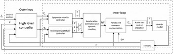
To solve the trajectory tracking problem, a two-level controller is proposed in Fig. 2. It is shown that the high-level controller can be considered as a guidance control to perform trajectory tracking function and generate attitude and velocity commands for the low-level controller. The low-level controller (the inner loop) can be regarded as an autopilot with stability augmentation system to stabilise the airship attitude and to track the desired velocity. The structure of the VBTTC includes a vectorial backstepping–based attitude controller, a CLF-based velocity controller, a virtual control calculation module and an active-set control allocation module. Next we will present the control design in detail.
Block diagram of the VBTTC architecture.

3.1 Vectorial backstepping method–based attitude controller
Consider the kinematic Equation (1). The attitude controller is derived in three steps.
Step 1 (Coordinate transformation). Two tracking error vectors of attitudes are defined as
 $$\begin{equation}
{z_1} \buildrel \Delta \over = \eta - {\eta _d},
\end{equation}$$
 $$\begin{equation}
{z_2} \buildrel \Delta \over = \dot{\eta } - {\dot{\eta }_r} = J\omega - \alpha
\end{equation}$$
where
 ${\dot{\eta }_r}$
represents the reference or virtual angular rate vector, Jω is the virtual control vector of
z
1.α is the stabilising function selected as the virtual angular rate vector of
 ${\dot{\eta }_r}$
. The derivatives of
z
1 and
z
2 are
 $$\begin{equation}
{\dot{z}_1} \buildrel \Delta \over = \dot{\eta } - {\dot{\eta }_d} = J\omega - {\dot{\eta }_d}
\end{equation}$$
 $$\begin{equation}
{\dot{z}_2} \buildrel \Delta \over = \ddot{\eta } - {\ddot{\eta }_r} = \dot{J}\omega - J\dot{\omega } - \dot{\alpha }
\end{equation}$$
Step 2 (Convergence of z 1). A CLF V 1 is constructed as follows:
 $$\begin{equation}
{V_1} = \frac{1}{2}z_1^T{z_1}
\end{equation}$$
Considering Equation (8), the derivative of V 1 is
 $$\begin{equation}
{\skew4\dot{V}_1} = z_1^T{\dot{z}_1} = z_1^T(J\omega - {\dot{\eta }_d})
\end{equation}$$
If Jω = α, the following stabilising function can be chosen to make the error system stable:
 $$\begin{equation}
\alpha = {\dot{\eta }_d} - {K_1}{z_1},
\end{equation}$$
where K 1 > 0 is often chosen as a diagonal matrix to simplify the design, so K 1 = diag(k11 , k12 , k13 ). However, there exists z 2 with z 2 ≠ 0, so the derivative of the first CLF of Equation (10) has to be modified by Equations (7) and (12) as
 $$\begin{equation}
{\skew4\dot{V}_1} = z_1^T{\dot{z}_1} = z_1^T({z_2} + \alpha - {\dot{\eta }_d}) = z_1^T({z_2} - {K_1}{z_1}) = - z_1^T{K_1}{z_1} + z_1^T{z_2}
\end{equation}$$
Step 3 (Backstepping for the variant of z 2). Define the second CLF as
 $$\begin{equation}
{V_2} = {V_1} + \frac{1}{{2c}}z_2^T{z_2},
\end{equation}$$
where c > 0 is a positive constant.
Differentiating Equation (12) with respect to time, we have
 $$\begin{equation}
\dot{\alpha } = {\ddot{\eta }_d} - {K_1}{\dot{z}_1}
\end{equation}$$
Considering Equation (13) and substituting Equations (9) and (15) into the derivative of V 2 yields
 $$\begin{equation}
{\skew4\dot{V}_2} = z_1^T{\dot{z}_1} + \frac{1}{c}z_2^T{\dot{z}_2} = - z_1^T{K_1}{z_1} + z_1^T{z_2} + \frac{1}{c}z_2^T(\dot{J}\omega + J\dot{\omega } - {\ddot{\eta }_d} + {K_1}{\dot{z}_1})
\end{equation}$$
A desired angular acceleration vector is selected as follows to make Equation (16) negative definite according to the Lyapunov theory,
 $$\begin{equation}
\dot{\Omega } = {J^{ - 1}}({K_2}{z_2} - \dot{J}\omega + {\ddot{\eta }_d} - c{z_1} - {K_1}{\dot{z}_1}),
\end{equation}$$
where K 2 = diag(k21 k22 k23 ) > 0, and the inversion and derivative of matrix J are as follows,
 $$\begin{equation*}
{J^{ - 1}} = \left( {\arraycolsep5pt\begin{array}{@{}*{3}{c}@{}} 1&0&{ - \sin \theta }\\ 0&{\cos \phi }&{\sin \phi \cos \theta }\\ 0&{ - \sin \phi }&{\cos \phi \cos \theta } \end{array}} \right),
\end{equation*}$$
 $$\begin{equation*}
\dot{J} = \frac{1}{{\cos \phi }}\left( {\arraycolsep5pt\begin{array}{@{}*{3}{c}@{}} 0&{\dot{\phi }\cos \phi \sin \theta + \dot{\theta }\sin \theta \sec \theta }&{\dot{\phi }\sin \phi \sin \theta + \dot{\theta }\cos \phi \sec \theta }\\ 0&{ - \dot{\phi }\sin \phi \cos \theta }&{ - \dot{\phi }\cos \phi \cos \theta }\\ 0&{ - \dot{\phi }\cos \phi + \dot{\theta }\sin \phi \tan \theta }&{ - \dot{\phi }\sin \phi + \dot{\theta }\cos \phi \tan \theta } \end{array}} \right)
\end{equation*}$$
From Equation (13), the following equation can be deduced,
 $$\begin{equation}
{z_2} = {\dot{z}_1} + {K_1}{z_1}
\end{equation}$$
Substituting Equation (18) into Equation (17) yields the following non-linear PD attitude control law:
 $$\begin{equation}
\dot{\Omega } = {J^{ - 1}}[ - \overbrace {({K_1}{K_2} + c{I_3})}^{{K_P}}{z_1} - \overbrace {({K_1} + {K_2})}^{{K_D}}{\dot{z}_1} - \dot{J}\omega + {\ddot{\eta }_d}],
\end{equation}$$
where K P = diag(kP1 , kP2,kP3 ) > 0, and K D = diag(kD1 , kD2 , kD3 ) > 0.
Substituting Equations (6) and (8) into Equation (19), the following control law is obtained:
 $$\begin{equation}
\dot{\Omega } = {J^{ - 1}}[{K_p}({\eta _d} - \eta ) + {K_D}({\dot{\eta }_d} - J\omega ) - \dot{J}\omega + {\ddot{\eta }_d}]
\end{equation}$$
3.2 CLF-based velocity controller design
Define a velocity tracking error vector as
 $$\begin{equation}
{z_3} \buildrel \Delta \over = \upsilon - {\upsilon _d},
\end{equation}$$
and the associated CLF is
 $$\begin{equation}
{V_3} = \frac{1}{2}z_3^T{z_3}.
\end{equation}$$
Differentiating Equation (22) with respect to time, we obtain
 $$\begin{equation}
{\skew4\dot{V}_3} = z_3^T{\dot{z}_3} = z_3^T(\dot{\upsilon } - {\dot{\upsilon }_d}).
\end{equation}$$
To stabilise the closed-loop system, according to the Lyapunov theory,
 ${\skew4\dot{V}_3}$
is required to be negative definite, so the following desired linear acceleration vector is obtained:
 $$\begin{equation}
\dot{\Xi } = {\dot{\upsilon }_d} - {K_3}{z_3} = {\dot{\upsilon }_d} + {K_3}{\upsilon _d} - {K_3}\upsilon ,
\end{equation}$$
where K 3 = diag(k 31, k 32, k 33) > 0.
Remark 1. The parameters
 $\upsilon \in {\mathbb{R}^2}$
,
 ${\upsilon _d} \in {\mathbb{R}^2}$
, and
 ${K_3} \in {\mathbb{R}^{2 \times 2}}$
(for Cases 1 and 2).
 $\eta \in {\mathbb{R}^2}$
,
 ${\eta _d} \in {\mathbb{R}^2}$
,
 $\omega \in {\mathbb{R}^2}$
, and
 ${K_P} \in {\mathbb{R}^{2 \times 2}}$
,
 ${K_D} \in {\mathbb{R}^{2 \times 2}}$
,
 $J \in {\mathbb{R}^{2 \times 2}}$
(for Case 2).
3.3 Calculation of the virtual control inputs
To accurately calculate the virtual control inputs under condition of under-actuated cases, the acceleration control law should be modified first. Two cases as in Section 2.2 are considered here.
For Case 1, the lateral acceleration
 $\dot{v}$
in Equation (24) cannot be directly used. By using the coupling relation of motion described in Equation (3), the value for
 $\dot{v}$
can be found to make the desired control force in y-direction vanish, that is,
 $$\begin{equation}
{f_{CPy}} = 0,
\end{equation}$$
where the dynamics equation of the control force in y-direction is
 $$\begin{equation}
{f_{CPy}} = {m_y}\dot{v} - m{z_G}\dot{p} + m{x_G}\dot{r} - {f_{dy}} - {f_{GBy}} - {f_{Ay}}.
\end{equation}$$
Since
 $\dot{p}$
and
 $\dot{r}$
are known control laws in Equation (20), the control law
 $\dot{v}$
is modified as follows:
 $$\begin{equation}
{\dot{v}_m} = \frac{m}{{{m_y}}}\left({z_G}\dot{p} - {x_G}\dot{r} + \frac{{{f_{dy}} + {f_{GBy}} + {f_{Ay}}}}{m}\right)
\end{equation}$$
For Case 2, it can be found that the acceleration of
 $\dot{p}$
in Equation (20) and
 $\dot{v}$
in Equation (24) cannot be directly used. So it is necessary to find a value for
 $\dot{v}$
and
 $\dot{p}$
simultaneously, which makes the desired side force and roll moment vanish, so we have
 $$\begin{equation}
{f_{CPy}} = {n_{CPx}} = 0,
\end{equation}$$
where the dynamics equations are
 $$\begin{equation}
\left\{ \arraycolsep5pt\begin{array}{@{}l@{}} {f_{CPy}} = {m_y}\dot{v} - m{z_G}\dot{p} + m{x_G}\dot{r} - {f_{dy}} - {f_{GBy}} - {f_{Ay}}\\ {n_{CPx}} = - m{z_G}\dot{v} + {J_x}\dot{p} - {J_{xz}}\dot{r} - {n_{dx}} - {n_{GBx}} - {n_{Ax}} \end{array} \right.
\end{equation}$$
Since the acceleration of
 $\dot{r}$
is known control law in Equation (20), the control laws of
 $\dot{v}$
and
 $\dot{p}$
are modified as
 $$\begin{equation}
{\dot{v}_m} = \frac{{({J_x}m{x_G} - {J_{xz}}m{z_G})\dot{r} - {J_x}({f_{dy}} + {f_{GBy}} + {f_{Ay}}) - m{z_G}({n_{dx}} + {n_{GBx}} + {n_{Ax}})}}{{{m^2}{z_G}^2 - {J_x}{m_y}}},
\end{equation}$$
 $$\begin{equation}
{\dot{p}_m} = \frac{{({m^2}{z_G}{x_G} - {J_{xz}}{m_y})\dot{r} - m{z_G}({f_{dy}} + f_{GBy} + f_{Ay}) - {m_y}({n_{dx}} + {n_{GBx}} + {n_{Ax}})}}{{{m^2}{z_G}^2 - {J_x}{m_y}}},
\end{equation}$$
when all the desired linear acceleration and angular acceleration control laws are obtained, the associated control forces and moments can be calculated by the following equation:
 $$\begin{equation}
{F_{CP}} = M\skew4\dot{V} - {F_d} - {F_{GB}} - {F_A},
\end{equation}$$
where
 $\skew4\dot{V} = {[ {\dot{u},{{\dot{v}}_m},\dot{w},\dot{p},\dot{q},\dot{r}} ]^T}$
for Case 1, and
 $\skew4\dot{V} = {[ {\dot{u},{{\dot{v}}_m},\dot{w},{{\dot{p}}_m},\dot{q},\dot{r}} ]^T}$
for Case 2.
3.4 VBTTC with active-set control allocation
To obtain the manipulating inputs, a control allocation problem is presented to solve Equation (4) with actuator saturation constraints:
 $$\begin{equation}
{F_{CP}} = Bu
\end{equation}$$
subject to
 $$\begin{equation}
\max (u(t - T) + {\dot{u}_{\min }}T,{u_{\min }}) = \underline u \le u \le \bar{u} = \min (u(t - T) + {\dot{u}_{\max }}T,{u_{\max }}),
\end{equation}$$
where
 $\underline u $
and
 $\bar{u}$
are lower and upper bounds of the actuator inputs.
According to control allocation principle(Reference Harkegard22), the problem of Equations (31) and (32) can be transformed into a constrained optimisation problem. The feasible solutions of the optimisation problem can be found by solving the following equation:
 $$\begin{equation}
{u_1} = \Omega = \arg \mathop {\min }\limits_{\underline u \le u \le \overline u } \left\| {{W_v}(Bu - {F_{CP}})} \right\|,
\end{equation}$$
where W v is the weighting matrix for prioritisation of virtual control channels. The 2-norm ‖u‖2 = uTu. The second objective is to find the optimal solution that is close to the desired control vector u d. The optimal solution u ∗ is found from Ω by solving the following equation:
 $$\begin{equation}
{u_s} = {u^ * } = \arg \mathop {\min }\limits_{u \in \Omega } \left\| {{W_u}(u - {u_d})} \right\|,
\end{equation}$$
where u d is generally selected as a zero vector(Reference Harkegard22), and Wu is the weighting matrix for prioritisation of actuators. For numerical efficiency, both objective functions of Equations (33) and (34) are merged into one objective:
 $$\begin{equation}
J = \left\| {{W_u}(u - {u_d})} \right\| + \gamma \left\| {{W_v}(Bu - {F_{CP}})} \right\|,
\end{equation}$$
where γ is chosen as a large number to emphasize the primary of error objective in the optimisation.
So the control allocation problem can be transformed into the above Weight Least Square (WLS) problem. And an Active Set Method (ASM) is proposed to solve the WLS problem with the actuator's saturation constraints. The algorithm of the ASM-based WLS control allocation is described as follows(Reference Harkegard22),
Phase 1:
-
1) Let u0 be a feasible initial point, which meets requirements of
(36)
$$\begin{equation}Bu = {F_{CP}},\end{equation}$$
(37)
$$\begin{equation}
Cu\geq U,C=[I,-I]^T,U=[u_{\rm max},-u_{\rm min}]^T.\end{equation}$$


Let ∏ be the working set and contain the active inequality constraint of Inequation (37) at u0.
-
2) For k = 0,1,2,. . ., N-1 (N is the maximum iteration number)
Given uk , find the optimal perburbation p, considering the constraints in the working set as equality constraints of Equation (36) and disregrading the remaining inequality constraints of Inequation (37).
Solve
 $$\begin{equation}
\arraycolsep5pt\begin{array}{@{}c@{}}
{u_1} = \min\limits_p \left\| {{W_v}\left( {B({u^k} + p) - {F_{CP}}} \right)} \right\|\\
{Bp = 0},\\
{p_i} = 0,i \in \prod \end{array}
\end{equation}$$
if uk +p is feasible.
Set uk +1 = uk +p, and compute the Lagrange multiplers{η lgr, λ lgr}, where η lgr is associate with Bu = F CP, and λ lgr with the active contraints of Cu ≥ U.
if all λ lgr ≥ 0
uk +1 is the optimal solution to Equation (33) subject to
 $$\begin{equation}
\arraycolsep5pt\begin{array}{@{}*{1}{c}@{}} {Bu = {F_{CP}}}\\ {Cu \ge U} \end{array},
\end{equation}$$
else
Remove the constraint associated with the most negative λ lgr from the working set.
else
Determine the maximal step length a, such that uk +1 = uk + ap is feasible. And add the primary bounding constraint to the working set.
end
-
3) If Bu 1 = F CP, then move to Phase 2; otherwise, set u s = u 1 and halt.
Phase 2:
-
1) Let u0 and ∏ be the solution and working set Ω resulted from Phase 1;
-
2) Solve following us by using the same method of Step 2 in Phase 1,
(40)
$$\begin{equation}{u_s} = {u^*} = \mathop {\arg \min }\limits_u \left\| {{W_u}\left( {u - {{\rm{u}}_d}} \right)} \right\|,\end{equation}$$

subject to
 $$\begin{equation}
Bu = {F_{CP}}{\rm{, }}{u_{\min }} \le u \le {u_{\max }}.
\end{equation}$$
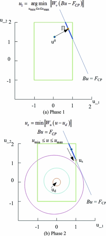
An illustration of the above active set control allocation procedure is shown Fig. 3, where control u has two inputs of u_1 and u_2 within range of (−1, 1).
Active set control allocation algorithm with two inputs.

Through the above control allocation algorithm, the active set–based control allocation module can be implemented and incorporated into the VBTTC scheme. When the optimal solution u s is found, the practical control input signals, including thrust force, tilt angle and control surface deflections, are obtained.
3.5 High-level controller design
The high-level controller provides airship guidance capability through a predefined trajectory. It generates the desired commands for airship attitude as well as desired velocities in x and z direction in F b, which is used for the low-level controller.
The high-level controller is designed by using a virtual reference vehicle that moves from waypoint to waypoint in a straight line at a pre-defined speed. As the controller starts, the reference vehicle moves along a straight line from the current airship to the first waypoint, and it stops at each waypoint until the airship is within a certain distance from the waypoint. As soon as the airship moves into this range, the reference vehicle resumes travel to next waypoint.
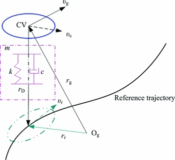
The airship desired attitude η
d
and velocity in Fb
can be calculated by using the vehicle reference velocity
 ${\upsilon _r}$
and the current distance rD
between the airship and the reference vehicle (see Fig. 4). According to the virtual spring damping principle, the desired or commanded velocity
 ${\dot{\upsilon }_c}$
in Fg
is first obtained by the following differential equation(Reference Liesk, Nahon and Boulet23):
 $$\begin{equation}
{\dot{\upsilon }_c} = {\sigma _2}({\upsilon _r} - {\upsilon _c} + {\sigma _1}({r_r} - {r_g})) + {\upsilon _r},
\end{equation}$$
where σ
1
> 0 and σ
2
> 0 are the controller design parameters. σ
1 . σ
2 represents the spring stiffness coefficient, σ
2 denotes the damping coefficient, r
g is the position of the actual airship and
 ${\upsilon _g}$
is the actual airship velocity in Fg
.
The virtual spring-damper system used for trajectory tracking.

It can be seen that the desired tracking trajectory ξ
d
meets
 ${\dot{\xi }_d} = {\upsilon _c}$
. And the high-level controller needs to transform the desired velocity vector in the body frame as well as the desired attitude. The desired velocity vector in F
g can be rewritten as
 ${\upsilon _c} = {[ {\arraycolsep5pt\begin{array}{*{20}{c}} {{u_{dg}}}&{{v_{dg}}}&{{w_{dg}}} \end{array}} ]^T}$
.
The desired velocities of u db and w db in F b can be computed as
 $$\begin{equation}
\left[ {\arraycolsep5pt\begin{array}{@{}*{1}{c}@{}} {{u_{db}}}\\ {{w_{db}}} \end{array}} \right] = \left[ {\arraycolsep5pt\begin{array}{@{}*{3}{c}@{}} 1&0&0\\ 0&0&1 \end{array}} \right]\bm{R}\left( \eta \right) \cdot {\upsilon _c},
\end{equation}$$
where R is direction cosine matrix of Equation (2). And the desired horizontal components of the velocity and flight-path azimuth angle χ are as follows,
 $$\begin{equation}
{u_{d\_{\rm{hor}}}} = \sqrt {u_{dg}^2 + v_{dg}^2} ,\;{\chi _{d\_{\rm{hor}}}} = {\tan ^{ - 1}}\frac{{{v_{dg}}}}{{{u_{dg}}}},
\end{equation}$$
and the desired velocity in the direction of the airship heading can be obtained as
 $$\begin{equation}
{u_{d\_{\rm{head}}}} = {u_{d\_{\rm{hor}}}}\cos \left( {{\chi _{d\_{\rm{hor}}}} - \psi } \right),
\end{equation}$$
where ψ is the current yaw angle.
The desired pitch angle can be obtained by the desired velocity vector and its horizontal projection, that is,
 $$\begin{equation}
{\theta _d} = {\tan ^{ - 1}}\frac{{{w_{dg}}}}{{{u_{d\_{\rm{hor}}}}}}.
\end{equation}$$
The desired roll angle and yaw rate are calculated by using the lateral velocity error
 $\tilde{v}$
in the body frame, the lateral velocity error corresponds to the difference between desired and actual velocity in body y-direction and is presented by
 $$\begin{equation}
\tilde{v} = \left[ {\arraycolsep5pt\begin{array}{*{20}{c}} 0&1&0 \end{array}} \right]\bm{R}\left( \eta \right)\left( {{v_{dg}} - {v_g}} \right).
\end{equation}$$
The desired roll angle and yaw rate are provided as follows,
 $$\begin{equation}
\left\{ \arraycolsep5pt\begin{array}{@{}l@{}} {\phi _d} = {c_\phi }\tilde{v}\\ {{\dot{\psi }}_d} = {c_\psi }\tilde{v} \end{array} \right..
\end{equation}$$
Remark 2. For under-actuated airships, the desired attitude η
d
and velocity
 ${\upsilon _d}$
generated by the high level controller are part of the whole vector, that is, Case 1:
 ${\upsilon _d}$
= (udb
, wdb
)T,
η
d
= (ϕd, θd, ψd
)T; Case 2:
 ${\upsilon _d}$
= (udb
, wdb
)T,
η
d
= (θd, ψd
)T.
3.6 Stability analysis
Lemma 1
(Reference Khalil28). Consider the non-linear system
 $\dot{x}(t)$
= f (
x
(t)) with the equilibrium point
x
= 0. Let
 $V(x):\mathbb{C} \to \mathbb{R}$
be a continuously differentiable positive definite function such that for
x
∈
 $\mathbb{C}$
(
 $\mathbb{C} \subset {\mathbb{R}^n}$
)
 $$\begin{equation}
{k_1}{\left\| x \right\|^b} \le V(x) \le {k_2}{\left\| x \right\|^b},
\end{equation}$$
 $$\begin{equation}
\skew4\dot{V}(x) = \frac{{\partial V}}{{\partial x}}f(x) \le - {k_3}{\left\| x \right\|^b},
\end{equation}$$
where k
1
, k
2
, k
3 and
 $b \in {\mathbb{R}^ + }$
are given constants. If Inequalities (49) and (50) hold for all initial states
 $x(0) \in {\mathbb{R}^n}$
, then
x
= 0 is globally exponentially stable.
Theorem 1. Consider the system of Equations (1), (2) and (3). Assume that (A1) the desired trajectory
 ${\xi _d}(t):[0,\infty ) \to {\mathbb{R}^3}$
is sufficiently smooth with its time-derivatives (
 ${\upsilon _r}(t) = {\dot{\xi }_d}(t)$
,
 ${\dot{\upsilon }_r}(t)$
) bounded; (A2) the output signal
 ${\upsilon _g}(t)$
tracks the commanded signal
 ${\upsilon _c}(t)$
in Equation (42) without steady tracking error, i.e.,
 $\mathop {\lim }\limits_{t \to \infty } {\upsilon _g}(t) = \mathop {\lim }\limits_{t \to \infty } {\upsilon _c}(t)$
. The VBTTC, given by Equations (20), (24) and (30), can guarantee global exponential stability of the tracking error dynamics of attitude, velocity and position.
Proof. Construct the following Lyapunov function for the entire system in accordance with Equations (14) and (22):
 $$\begin{equation}
V = {V_l} + {V_h} = \frac{1}{2}z_1^T{z_1} + \frac{1}{{2c}}z_2^T{z_2} + \frac{1}{2}z_3^T{z_3} + \frac{1}{2}z_4^TP{z_4},
\end{equation}$$
where zi (i = 1, 2, 3, 4) are the tracking error vectors defined in Section 3.1 and 3.2. P is positive definite for sufficiently small values of ε.
The Lyapunov function for the high-level controller in Equation (51) is as follows:
 $$\begin{equation}
{V_h} \buildrel \Delta \over = \frac{1}{2}z_4^TP{z_4},
\end{equation}$$
where
 ${z_4} = \left( {\arraycolsep5pt\begin{array}{@{}*{1}{c}@{}} {{\xi _d} - \xi }\\ {{\upsilon _r} - {\upsilon _c}} \end{array}} \right)$
,
 $P = \left( {\arraycolsep5pt\begin{array}{@{}*{2}{c}@{}} 1&{\frac{\varepsilon }{{{\sigma _1}{\sigma _2}}}}\\ {\frac{\varepsilon }{{{\sigma _1}{\sigma _2}}}}&{\frac{1}{{{\sigma _1}{\sigma _2}}}} \end{array}} \right)$
, σ
1 andσ
2 are parameters in Equation (42).
Differentiating Equation (52) and considering Equation (42) with
 ${\upsilon _g} = {\upsilon _c}$
and
 ${\upsilon _g} = \dot{\xi }$
yields
 $$\begin{equation}
{\skew4\dot{V}_h} = z_4^T\left( {\arraycolsep5pt\begin{array}{@{}*{2}{c}@{}} 0&{ - {\sigma _1}{\sigma _2}}\\ 1&{ - {\sigma _2}} \end{array}} \right)P{z_4} \buildrel \Delta \over = - z_4^TQ{z_4},
\end{equation}$$
where
 $Q = \left( {\arraycolsep5pt\begin{array}{@{}*{2}{c}@{}} \varepsilon &{\frac{\varepsilon }{{2{\sigma _1}}}}\\ {\frac{\varepsilon }{{2{\sigma _1}}}}&{\frac{{{\sigma _2} - \varepsilon }}{{{\sigma _1}{\sigma _2}}}} \end{array}} \right)$
. Subsituting Equations (17) and (24) into
 $\skew4\dot{V}$
, we have
 $$\begin{equation}
\begin{array}{l}
\skew4\dot{V} = - z_1^T{K_1}{z_1} + z_1^T{z_2} + \frac{1}{c}z_2^T(\dot{J}\omega + J\dot{\omega } - {{\ddot{\eta }}_d} + {K_1}{{\dot{z}}_1}) + z_3^T(\dot{\upsilon } - {{\dot{\upsilon }}_d}) - z_4^TQ{z_4}\\
\hphantom{\skew4\dot{V}} = - z_1^T{K_1}{z_1} - \frac{1}{c}z_2^T{K_2}{z_2} - z_3^T{K_3}{z_3} - z_4^TQ{z_4}\\
\hphantom{\skew4\dot{V}} \buildrel \Delta \over = - {z^T}\Lambda z\,\,,\\
\hphantom{\skew4\dot{V}} \le - {\lambda _{\min }}(\Lambda ){z^T}z\\
\end{array}
\end{equation}$$
where
Ʌ
= K
1+K
2+K
3+Q, λmin
(
Ʌ
) is the minimum eigenvalue of
Ʌ
. Since
Ʌ
is positive definite,
 $\skew4\dot{V}$
is negative definite. According to Lemma 1, the system is globally exponentially stable at
z
= 0, where the exponent b = 2. Thus, the desired trajectory ξ
d
is precisely tracked with
 $\mathop {\lim }\limits_{t \to \infty } \| {\xi (t) - {\xi _d}(t)} \| = 0$
.
Remark 3. According to Theorem 1, state variables of η, ω, ξ and
 $\upsilon $
are bounded. Although the side-sway velocity v is not directly controlled, it can be proved bounded. The proof procedure is inspired by Proposition 2 in Reference Zheng and WuRef. 19. For Case 1, considering the aerodynamic force described in Reference Mueller, Paluszek and ZhaoRef. 24, we have
 $$\begin{equation}
\begin{array}{@{}l@{}}
\dot{v} = \frac{m}{{{m_y}}}\left( {{z_G}\dot{p} - {x_G}\dot{r} + \frac{{{f_{dy}} + {f_{GBy}} + {f_{Ay}}}}{m}} \right)\\
\hphantom{\dot{v}} = \frac{{\bar{q}}}{{{m_y}}}({C_{y1}}\cos (\beta /2)\sin (2\beta ) + {C_{y2}}\sin (2\beta ) + {C_{y3}}\sin (\beta )\sin \left| \beta \right|) + {b_1}\\
\hphantom{\dot{v}}= \frac{1}{{2{m_y}}}\rho (u_c^2 + {v^2})({C_{y1}}\cos (\beta /2)\frac{{2{u_c}v}}{{u_c^2 + {v^2}}} + {C_{y2}}\frac{{2{u_c}v}}{{u_c^2 + {v^2}}} + {C_{y3}}\frac{v}{{\sqrt {u_c^2 + {v^2}} }}\sin \left| \beta \right|) + {b_1},\\
\hphantom{\dot{v}}\approx \frac{\rho }{{{m_y}}}{u_c}({C_{y1}}\cos (\beta /2) + {C_{y2}} + \frac{1}{2}{C_{y3}}\sin \left| \beta \right|)v + {b_1}\\
\hphantom{\dot{v}}\buildrel \Delta \over = - {a_1}v + {b_1} \end{array}
\end{equation}$$
where
 $$\begin{equation}
\arraycolsep5pt\begin{array}{@{}*{1}{l}@{}} {{a_1} = - \displaystyle\frac{\rho }{{{m_y}}}{u_c}({C_{y1}}\cos (\beta /2) + {C_{y2}} + \frac{1}{2}{C_{y3}}\sin \left| \beta \right|)}\\
{{b_1} = \displaystyle\frac{1}{{{m_y}}}[m{z_G}\dot{p} - m{x_G}\dot{r} - {m_x}ur + {m_z}\omega p - m{z_G}qr - m{x_G}pq + (G - B)\cos \theta \sin \phi ]} \end{array},
\end{equation}$$
 $$\begin{equation}
\beta = \arctan 2(v,{u_c}) \in \left( - \frac{\pi }{2},\frac{\pi }{2}\right),\;u_c^2 = {u^2} + {w^2},
\end{equation}$$
When attitude and angular rates dynamics are all well regulated, b
1 becomes a constant value. Considering uc > 0,Cy
2
< 0, Cy
3
< 0, |Cy
2
| > |Cy
1|, ρ>0, my > 0, cos (β/2) > 0 and sin |β| > 0, we have a
1
> 0. From the above equations, it can be seen that the sway velocity is bounded and
 $\mathop {\lim }\limits_{t \to \infty } v(t) = {b_1}/{a_1}$
.
For Case 2, ϕ is bounded due to roll subsidence mode, and v can also be proved bounded by similar method. Therefore, all the state variables are bounded in the VBTTC scheme.
4.0 SIMULATION RESULTS AND ANALYSIS
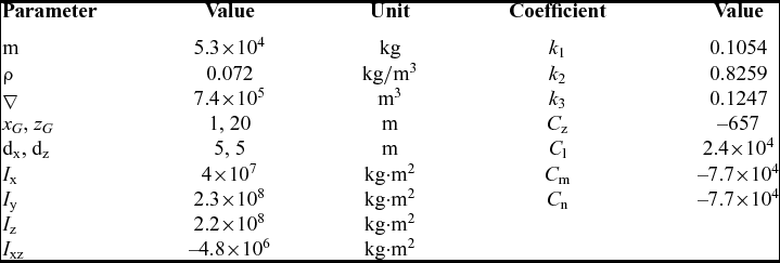
The physical parameters and aerodynamic control coefficients of the stratospheric airship are shown in Table 1 (Reference Mueller, Paluszek and Zhao24). Controller parameters for Cases 1 and 2 are designed as follows:
 $$\begin{equation}
\arraycolsep5pt\begin{array}{@{}*{1}{c}@{}} {{\sigma _1} = 0.1{\rm{ }}\left[ {\displaystyle\frac{1}{s}} \right],{\sigma _2} = 0.2{\rm{ }}\left[ {\displaystyle\frac{1}{s}} \right],{c_\phi } = 1{\rm{ }}\left[ {\displaystyle\frac{{\deg \cdot s}}{{\rm{m}}}} \right],{c_\psi } = 12{\rm{ }}\left[ {\displaystyle\frac{{\deg \cdot s}}{{\rm{m}}}} \right]}\\ {{K_P} = {K_D} = 4{I_3},{K_3} = 4{I_2},\gamma = 1 \times {{10}^6},{W_v} = {I_5},{W_u} = {I_6}} \end{array},\quad \left( {{\rm{Case}}\;1} \right)
\end{equation}$$
 $$\begin{equation}
\arraycolsep5pt\begin{array}{@{}*{1}{c}@{}} {{\sigma _1} = 0.1{\rm{ }}\left[ {\displaystyle\frac{1}{s}} \right],{\sigma _2} = 0.2{\rm{ }}\left[ {\displaystyle\frac{1}{s}} \right], {c_\psi } = 12{\rm{ }}\left[ {\displaystyle\frac{{\deg \cdot s}}{{\rm{m}}}} \right]}\\ {{K_P} = {K_D} = {K_3} = 4{I_2},\gamma = 1 \times {{10}^6},{W_v} = {I_4},{W_u} = {I_4}} \end{array}\hspace*{-8pt},\quad \left( {{\rm{Case}}\;2} \right)
\end{equation}$$
where KP , KD and K 3 are selected to satisfy the requirements in Section 3 after several design iterations. I n denotes the unit matrix with n dimensions.
Parameters and coefficients for the demo airship

The position constraints for the actuators are (−25°, 25°), and their rate constraints are(−80°/s, 80°/s). The initial position of the airship is ξ0 = (0, 0, −20,000 m)T, initial velocity in Fb is v 0 = (18 m/s, 0, 0)T, initial attitude is η 0 = (0, 0, 0)T, and initial angular velocity is ω 0 = (0, 0, 0)T.
4.1 Attitude tracking control
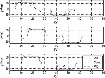
To verify the effectiveness of attitude controller, attitude commands of doublet inputs r = ±60° are set when the forward velocity u is regulated at 18 m/s and the vertical velocity w is stabilised at zero. The roll command of ϕd starts at t = 5s, the yaw command of ψd starts at t = 10 s, and the pitch command θd starts at t = 15 s. A PID controller, with controller parameters of KP = 4, KI = 0.1 and KD = 4 in the three channels of roll, pitch and yaw, is used to compare with the VBTTC method. Meanwhile, to observe the robustness of the proposed controller, the aerodynamic coefficients of the airship are given 30% uncertainties. The external disturbances of force and moment are set as fr (t) = 500sin(2πt)× I 3 N and nr (t) = 500sin(2πt)× I 3 N·m.
Simulation results are shown in Fig. 5. It can be seen that the vectorial backstepping (VB)–based attitude controller shows much better tracking performances than those by using PID controller. The conventional PID controller tends to have large overshoot. And the uncertainties and disturbances have little influence on the VB attitude controller due to the robustness of backstepping method, while the performances of the PID scheme severely deteriorate.
Attitude tracking responses of doublet inputs.

4.2 Attitude control with control allocation
To show control allocation performances, a Direct Control Allocation (DCA) by solving the Linear Programming (LP) is applied to comparing with the active set allocation method. The DCA method is an optimisation as following,
 $$\begin{equation}
\mathop {\max }\limits_{\underline u \le u \le \overline u } a\;{\rm{subject\; to}}\; Bu = av,
\end{equation}$$
if a>1, set u = u/a, a denotes scaling factor.
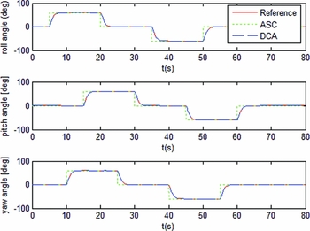
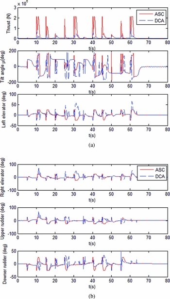
The same doublet commands of the attitudes as Section 4.1, and the output tracking responses are shown as Fig. 6. It can be seen that both controllers of VB with active set control (ASC) allocation and VB with DCA can well track the commands. However, there is obvious difference in control inputs (see Fig. 7); ASC allocation uses small inputs of control surfaces deflection with a big thrust, while DCA applies large inputs of control surfaces deflection with a small thrust, which will result a big drag and more energy consumption.
Attitude tracking responses.

Control inputs for attitude tracking control comparing ASC with DCA allocation.

4.3 Trajectory tracking control
A helix trajectory is predefined as the desired trajectory to verify the tracking performance of the VBTTC. The desired trajectory function is performed as
 $$\begin{equation}
{\xi _d}(t) = {[{x_d},{y_d},{z_d}]^T} = \int\limits_0^t {{{\dot{\xi }}_d}(t)d\tau } + {\xi _{d0}},
\end{equation}$$
where
 ${\dot{\xi }_d}(t) = {\upsilon _r} = {[V\cos (\frac{{2\pi }}{T}t),V\sin (\frac{{2\pi }}{T}t), - {V_z}]^T}$
and initial position ξ
d0 = [40m, −50m, −19960m]
T
are velocity function and initial position of the desired trajectory, respectively. The horizontal speed for tracking is V = 20 m/s, the ascending speed is Vz
= 1 m/s, and the motion period is T = 300 s.
Scenario I:
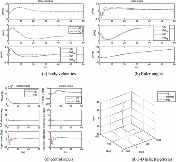
Case 1 is considered and the control parameters are designed as in Equation (46). To compare the controller performance, this scenario is also simulated by using the PID controller in attitude control loop described as Section 4.1. And parameters in the guidance loop are designed as Equation (58). The simulation results are shown in Fig. 8. From Fig. 8(a), Fig. 8(b) and Fig. 8(d), it is observed that the desired trajectory and reference velocities and attitudes are well tracked by VB and PID control, and their tracking errors converge to the origin in 60s. Since the references of vertical velocity and roll angle in the guidance loop using the VB control are greater than those using the PID method, the resulted control inputs of tilt angle of the thrusters and rudders fluctuate more violently for VB.
Responses of trajectory tracking control comparing VB with PID.

Scenario II:
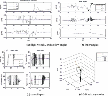
Case 2 is considered and the control parameters are designed as in Equation (47). To observe the controller robust performance, this scenario is simulated with time delay of the actuators, and the problem of robust control of the airship with state delays was studied in Reference Liu, Li and JinRef. 29. Three different time delays are considered, i.e., G τ(s) = 1/(τs + 1) with τ = 0, τ = 0.2s and τ = 0.6s. The parameters in the guidance loop and the autopilot loop are designed as Equation (59). The 3D reference trajectory and its trajectory tracking responses are shown in Fig. 9. It can be seen from Fig. 9, with the increasing of time delay, the tracking outputs of attitude angles and flight velocity begin oscillation and instability, and the control inputs are up to saturation. Therefore, time delay of the actuator makes the control system performance deteriorate and even to instability.
Responses of trajectory tracking control with different time delays of actuators.

From Figs 8(b) and 9(b), it can be seen that the bank angle Φ in Case 1 is smaller than that in Case 2 without time delay. Since the roll moment is actuated in Case 1, the desired bank angle can be tracked with good damping. And side-slipping angles of both cases are bounded, which implies that the sway velocities of both cases are bounded. The simulation results are in accordance with Theorem 1 and Remark 3.
5.0 CONCLUSION
A new control approach for the under-actuated stratospheric airship is developed to track a flight trajectory in 3D space. Based on a full 6-DOF non-linear model, the trajectory tracking controller is designed in two levels. The low-level controller stabilises the attitude and velocity of the airship via the non-linear VB method, and then the high-level controller performs the autonomous trajectory tracking task. Furthermore, the control allocation module based on the active set algorithm is incorporated into the low-level controller to optimise the real control inputs under constraints of saturation. Stability analysis and simulation results show that the closed-loop trajectory tracking error dynamics are globally exponentially stable. Compared with the conventional PID controller, the VBTTC designed for two cases of the under-actuated airship can achieve better trajectory tracking performances even though the airship is affected by parametric uncertainties and exogenous disturbances. Therefore, the effectiveness and availability of the VBTTC design are validated.
ACKNOWLEDGEMENTS
This work has been funded by the Chinese special research program of a large civil aircraft under the Grant MJZ-S-2011-06, MJZ-2015-S-080, the Chinese Aviation Science Fund under the Grant 20160757001, and the National Natural Science Fund under the Grant 10577012. The authors would like to thank the associate editor and anonymous reviewers for their valuable comments and suggestions.