


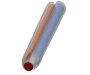



1. Introduction
From the flight of dandelion seeds transported by the wind to phytoplankton settling in the ocean, the prediction of bifurcations resulting from fluid–solid interactions on a freely falling object is a fascinating subject, with countless applications spanning from meteorology, ecology and insect flight to engineering applications (see Ern et al. (Reference Ern, Risso, Fabre and Magnaudet2012) for a review). The interactions between wake and free-fall dynamics have been widely investigated in the literature. Everyday objects such as paper sheets show several falling paths, such as fluttering and tumbling trajectories, faithfully reproduced by ordinary differential equation (ODE) models which include aerodynamic interactions (Belmonte, Eisenberg & Moses Reference Belmonte, Eisenberg and Moses1998; Pesavento & Wang Reference Pesavento and Wang2004; Andersen, Pesavento & Wang Reference Andersen, Pesavento and Wang2005). Similar zig-zag and oblique paths have been observed for buoyant drops and bubbles (Magnaudet, Rivero & Fabre Reference Magnaudet, Rivero and Fabre1995; Magnaudet & Eames Reference Magnaudet and Eames2000; Mougin & Magnaudet Reference Mougin and Magnaudet2001). Other relevant examples include particle settling and transport (Stringham, Simons & Guy Reference Stringham, Simons and Guy1969; Dietrich Reference Dietrich1982; Matas, Morris & Guazzelli Reference Matas, Morris and Guazzelli2004; Camenen Reference Camenen2007; Guazzelli, Morris & Pic Reference Guazzelli, Morris and Pic2011).
Buoyancy-driven disks have been the object of substantial interest in the fluid dynamics community since they present a great variety of falling paths, such as zig-zag, tumbling and chaotic motion (Willmarth, Hawk & Harvey Reference Willmarth, Hawk and Harvey1964; Field et al. Reference Field, Klaus, Moore and Nori1997; Fernandes et al. Reference Fernandes, Ern, Risso and Magnaudet2008). Auguste, Magnaudet & Fabre (Reference Auguste, Magnaudet and Fabre2013) performed an extensive numerical study, identifying several planar and non-planar falling paths, varying independently the fluid properties and disk inertia. The authors highlighted the influence of the disk thickness on the resulting falling trajectories. For disks of very small thickness, a relatively larger flow inertia leads to the transition from a steady vertical (SV) path to a zig-zag regime, characterized by very low-amplitude oscillations at low values of the disk inertia and large-amplitude oscillations at moderate and large disk inertia. For a ratio between the disk thickness and diameter of  $0.1$, the authors observed the transition from the SV path to a regime characterized by a steady oblique trajectory with a constant inclination of the disk, analogous to the one obtained by Fabre, Tchoufag & Magnaudet (Reference Fabre, Tchoufag and Magnaudet2012) via a weakly nonlinear expansion around the SV path.
However, direct numerical simulations suffer from being extremely costly in terms of computational time, in particular in parametric studies. The temporal transient becomes (virtually) infinitely long close to instability thresholds. From this perspective, a suitable approach to tackling large parametric studies and obtaining precise thresholds is linear stability analysis. This tool can provide the threshold value of the instability of a certain path with respect to perturbations as well as detailed information about the unstable neutral mode, in reasonable computational time (Assemat, Fabre & Magnaudet Reference Assemat, Fabre and Magnaudet2012). The advantage becomes striking when the stability of an axisymmetric state, e.g. the SV path, is considered. Exploiting the axisymmetry of the flow associated with the SV path, the three-dimensional problem can also be reduced to a two-dimensional one, with an enormous reduction of the computational times (cf. Meliga, Chomaz & Sipp (Reference Meliga, Chomaz and Sipp2009b) among others). As a consequence of the linearization of the governing equations, linear stability analysis, however, allows one to understand the emerging path only in the vicinity of the instability threshold and cannot give information on the nonlinear saturated state. The instability of the SV axisymmetry-preserving path was rationalized in Tchoufag, Fabre & Magnaudet (Reference Tchoufag, Fabre and Magnaudet2014) via a linear stability analysis exploiting a Fourier decomposition of the azimuthal perturbations. The SV path presents several instabilities, with azimuthal wavenumber  $m=\pm 1$, which depend on the considered disk inertia; three oscillatory and one non-oscillatory modes are identified. Although the related neutral curves, i.e. curves associated with a zero growth rate in the parameter space, often intersect, a threshold value of the Reynolds number could nevertheless be identified, below which the SV trajectory is stable. This value depends on the disk inertia. The authors also analysed the mutual coupling between the wake and disk dynamics by considering the qualitative differences between the real and imaginary parts of the modes, which represent the wake at two different instants of time within the period of oscillation of the mode. Strong re-organizations of the wake pattern imply a strong mutual coupling between wake and disk dynamics, associated with large-amplitude oscillations in the nonlinear simulations of Auguste et al. (Reference Auguste, Magnaudet and Fabre2013). These results were in quite good agreement with the observation of low- and large-amplitude zig-zag regimes. Besides, linear stability analysis predicted the onset of the steady oblique path for a disk of ratio thickness–diameter of 0.1, in very good agreement with the results of Auguste et al. (Reference Auguste, Magnaudet and Fabre2013). When two or more modes present similar thresholds, the dynamics results from a competition of the different modes (Fabre, Auguste & Magnaudet Reference Fabre, Auguste and Magnaudet2008), which cannot be unveiled only through linear stability analysis. In this case, weakly nonlinear analyses can shed light on the emerging trajectories or wake patterns, as performed by Meliga, Chomaz & Sipp (Reference Meliga, Chomaz and Sipp2009a), Citro et al. (Reference Citro, Tchoufag, Fabre, Giannetti and Luchini2016) and Sierra-Ausín et al. (Reference Sierra-Ausín, Lorite-Díez, Jiménez-González, Citro and Fabre2022) for the wake of fixed and rotating spheres.
Several falling objects such as dandelions are known to possess permeable structures (Cummins et al. Reference Cummins, Seale, Macente, Certini, Mastropaolo, Viola and Nakayama2018). The flow past a sufficiently permeable object may significantly differ from the one around a solid, impervious body, see e.g. Zong & Nepf (Reference Zong and Nepf2012) and Ciuti et al. (Reference Ciuti, Zampogna, Gallaire, Camarri and Ledda2021). Here, we focus on the behaviour of thin permeable objects. For Reynolds numbers of the order of  $Re \sim 10^4$, the wake flow past permeable plates exhibits a regime characterized by a steady wake region that extends far downstream of the body and a region further downstream associated with the vortex shedding, resulting in a detached mean recirculation region. For very large permeabilities, the vortex shedding is inhibited due to the air bleeding through the permeable body (Castro Reference Castro1971). This behaviour was confirmed in Ledda et al. (Reference Ledda, Siconolfi, Viola, Gallaire and Camarri2018) for
 $Re \sim 100$. The recirculation region past permeable plates abruptly detaches and shrinks at large permeability, and disappears. The increase in the critical Reynolds number for the onset of the von Kármán vortex street past the permeable object, obtained through linear stability analysis, becomes abrupt when approaching a critical value of the permeability, beyond which the linear instability is quenched. Similar flow features were observed in the case of thin permeable disks (Cummins et al. Reference Cummins, Viola, Mastropaolo and Nakayama2017; Ledda et al. Reference Ledda, Siconolfi, Viola, Camarri and Gallaire2019).
Flow around and through thin permeable objects may be computationally expensive due to the large range of length scales involved (Falcucci et al. Reference Falcucci, Amati, Fanelli, Krastev, Polverino, Porfiri and Succi2021) and potentially limited by the choice of a specific microscopic configuration. Homogenization provides insights into the modelling of flow through porous structures, rigorously establishing a link between the microstructure and its macroscopic effect on the large-scale flow (Hornung Reference Hornung1997; Zampogna & Bottaro Reference Zampogna and Bottaro2016; Lācis & Bagheri Reference Lācis and Bagheri2017). Homogenized models recover the macroscopic effects of the permeability and provide a formal framework to obtain these permeability properties from a microscopic structure, and vice versa (Ciuti et al. Reference Ciuti, Zampogna, Gallaire, Camarri and Ledda2021; Ledda et al. Reference Ledda, Boujo, Camarri, Gallaire and Zampogna2021). Therefore, the homogenized model does not suffer from the limitations stemming from the choice of a particular microscopic geometry. It also allows one to design specific microstructures which target the parameters used in the macroscopic boundary conditions. Thin permeable objects can be modelled as microstructured membranes, enabling the use of a homogenized model, which states that the velocity at the membrane is proportional to the difference of stresses across the membrane itself (Zampogna & Gallaire Reference Zampogna and Gallaire2020). The same model was validated in Ledda et al. (Reference Ledda, Boujo, Camarri, Gallaire and Zampogna2021) for  $Re \sim 100$.
While the buoyancy-driven instabilities of solid objects have been widely investigated in the literature, similar studies are lacking in the case of permeable structures. The prediction of the instability of trajectories of falling thin permeable objects is of significant interest owing to the large range of applications (Ern et al. Reference Ern, Risso, Fabre and Magnaudet2012), such as environmental ones (Cummins et al. Reference Cummins, Seale, Macente, Certini, Mastropaolo, Viola and Nakayama2018). Permeable disks are a suitable testing ground to investigate the role of permeability in modifying falling or rising trajectories of thin bodies. To this purpose, the combination of linear stability analysis and the homogenized model is suitable to perform a parametric study and give a first, unified, understanding of the path instability of a thin buoyancy-driven permeable disk. The employed formalism allows one to obtain general results, independent of a specific microscopic structure. Therefore, with the aim of unveiling the modifications induced by permeability to the rich picture of instabilities which characterize the rise or fall of a buoyancy-driven thin disk, we perform a linear stability analysis of the SV path with respect to azimuthal perturbations of a disk modelled as a thin permeable membrane. We predict the values of the parameters which ensure a stable steady, vertical path, and the emerging unstable trajectories. We begin by introducing the theoretical framework and numerical implementation. We then describe the flow features of the SV path and its instabilities as the permeability properties of the disk are varied.
2. Problem formulation
We consider a thin permeable disk composed of a periodic microstructure of characteristic length  $\ell$, as depicted in figure 1. We introduce the separation of scales parameter
 \begin{equation} \varepsilon=\frac{\ell}{D}, \end{equation}
where  $D$ is the disk diameter (see figure 1). The thickness of the disk is of the same order as the microscopic characteristic length, i.e.
 $h/D={O}(\varepsilon ) \ll D$. The disk is composed of a material of density
 $\rho _b$ and immersed in a viscous fluid of density
 $\rho$ and viscosity
 $\mu$; we denote with
 $\mathcal {V}$ its volume. We denote with
 $\bar {\boldsymbol {v}}(\bar {t})$ and
 $\bar {\boldsymbol {\varOmega }}(\bar {t})$ the translational and rotational velocities of the body during its trajectory, respectively. We introduce a Cartesian reference frame
 $(\bar {x},\bar {y},\bar {z})$ for Newton's equations, with origin on the disk centre and initially aligned with a fixed reference frame
 $(\bar {x}_1,\bar {x}_2,\bar {x}_3)$. In contrast, we employ cylindrical coordinates
 $(\bar {x},\bar {r},\bar {\varphi })$ for the incompressible Navier–Stokes equations for the flow dynamics (see figure 1). Following Tchoufag et al. (Reference Tchoufag, Fabre and Magnaudet2014), the flow equations are written in terms of absolute velocity, but with the above-defined coordinate systems rotating and translating with the disk. The
 $\bar {x}$-direction, common to both coordinate systems, is aligned along the disk axis.
 $(a)$ Sketch of the falling disk with relevant quantities and the employed reference frames, together with a sketch of a possible microscopic geometry with relative characteristic quantities.
 $(b)$ Sketch of the relative velocity recirculation region past a falling permeable disk.

The equations for the fluid–structure coupled problem are non-dimensionalized with the fall or rise velocity of the SV path  $U_{SV}$, stress
 $\rho U_{SV}^2$ and disk diameter
 $D$. We denote with
 $M=\rho _b \mathcal {V}$ the mass of the disk. Dropping bars for non-dimensional variables, the system of equations reads
 $$\begin{gather} \boldsymbol{\nabla} \boldsymbol{\cdot} \boldsymbol{u}=0,\quad \frac{\partial \boldsymbol{u}}{\partial t}+(\boldsymbol{u}-\boldsymbol{v}-\boldsymbol{\varOmega} \times \boldsymbol{r}) \boldsymbol{\nabla} \boldsymbol{u}+\boldsymbol{\varOmega} \times \boldsymbol{u}={-}\boldsymbol{\nabla} p+\frac{1}{R e} \nabla^{2} \boldsymbol{u}, \end{gather}$$
 $$\begin{gather}M^*\left(\frac{\mathrm{d} \boldsymbol{v}}{\mathrm{d} t}+\boldsymbol{\varOmega} \times \boldsymbol{v}\right)-\frac{M-\rho \mathcal{V}}{\rho D^2U_{SV}^2} \boldsymbol{g}=\int_{\varGamma_{int}} \varSigma(\boldsymbol{u}, p) \boldsymbol{n}\,\mathrm{d} \varGamma, \end{gather}$$
 $$\begin{gather}\boldsymbol{\mathsf{I}}^* \frac{\mathrm{d} \boldsymbol{\varOmega}}{\mathrm{d} t}+\boldsymbol{\varOmega} \times({\boldsymbol{I}}^*\boldsymbol{\varOmega})=\int_{\varGamma_{int}} \boldsymbol{r} \times[\varSigma(\boldsymbol{u}, p) \boldsymbol{n}]\, \mathrm{d} \varGamma,\quad \lim _{\|\boldsymbol{r}\| \rightarrow \infty} \boldsymbol{u}=0, \end{gather}$$
where  $\boldsymbol{g}$ is the gravity vector,
 ${\|\boldsymbol {r}\|}$ is the position vector from the disk centre,
 $\boldsymbol {n}$ is the normal to the considered boundary,
 $\varSigma _{ij}=-p\delta _{ij} +({1}/{Re})(\boldsymbol {\nabla } \boldsymbol {u})_{ij}$ is the non-dimensional stress tensor,
 $Re=({\rho U_{SV} D})/{\mu }$ is the Reynolds number defined with the disk diameter,
 $M^*{=M/(\rho D^3)}$ is the non-dimensional disk mass and
 ${\boldsymbol{\mathsf{I}}}^*$ is the dimensionless disk inertia tensor, whose non-zero components are
 ${\boldsymbol{\mathsf{I}}}^*_{xx}$ and
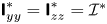 ${\boldsymbol{\mathsf{I}}}^*_{yy}={\boldsymbol{\mathsf{I}}}^*_{zz}=\mathcal {I}^*$. We also introduce the three angles describing the inclination of the disk
 $\boldsymbol {\vartheta }=(\vartheta _x,\vartheta _y,\vartheta _z)$, which are related to the angular velocity through the classical yaw–pitch–roll relations (Auguste Reference Auguste2010). Since the microstructure is not defined, the relation between the inertia tensor and the disk mass may differ from that of an impervious disk employed in Tchoufag et al. (Reference Tchoufag, Fabre and Magnaudet2014). The flow through the permeable microstructure is described via an interface condition that models the macroscopic drag induced by the microscopic solid structure, under the assumption of negligible flow inertia within the membrane pores. The model imposes a discontinuity in the fluid stresses and the continuity of velocity across the permeable membrane, whose surface is denoted as
 $\varGamma _{int}$ (red surface in figure 1b). Labelling with the superscripts
 $^-$ and
 $^+$ variables evaluated, respectively, on the upstream and downstream sides of the membrane of negligible thickness, as shown in figure 1, the generic interface conditions at the membrane
 $\varGamma _{int}$ read
 \begin{align} \boldsymbol{u}^+{-}\boldsymbol{v}-\boldsymbol{\varOmega} \times \boldsymbol{r}={Re}\left[ \boldsymbol{\mathsf{M}}\left[\varSigma\left(\boldsymbol{u}^{-}, p^{-}\right) \boldsymbol{n}^-\right]+\boldsymbol{\mathsf{N}}\left[\varSigma\left(\boldsymbol{u}^+, p^+\right) \boldsymbol{n}^+\right]\right], \quad \boldsymbol{u}^+ =\boldsymbol{u}^- \quad \text{on} \varGamma_{int},\end{align}
where  $\boldsymbol {u}-\boldsymbol {v}-\boldsymbol {\varOmega } \times \boldsymbol {r}$ is the relative velocity with respect to the membranal disk. The tensors
 $\boldsymbol{\mathsf{M}}$ and
 $\boldsymbol{\mathsf{N}}$ are, respectively, called upstream and downstream permeability tensors (Zampogna & Gallaire Reference Zampogna and Gallaire2020) and are non-dimensionalized by employing the macroscopic characteristic length, i.e. the diameter of the disk. These tensors result from microscopic Stokes-like problems around each repetitive element of the microstructure (detailed in Appendix A). They depend on the detailed geometry of the pores and are proportional to the separation of scales parameter
 $\varepsilon$. As shown in Ledda et al. (Reference Ledda, Boujo, Camarri, Gallaire and Zampogna2021), desired values of the components of
 $\boldsymbol{\mathsf{M}}$ and
 $\boldsymbol{\mathsf{N}}$ can be retrieved with a tailored combination of pore shape and size. Therefore, (2.3) is suitable to obtain results independent of a specific microstructure. We now focus on the case of a membrane composed of a homogenous and isotropic structure, symmetric with respect to the membrane mean surface. Under these assumptions, the macroscopic velocity at the membrane interface
 $\varGamma _{int}$ is given by
 \begin{equation} \boldsymbol{u}^+{-}\boldsymbol{v}-\boldsymbol{\varOmega} \times \boldsymbol{r}={Re} \boldsymbol{\mathsf{M}}\left[\varSigma\left(\boldsymbol{u}^{-}, p^{-}\right) \boldsymbol{n}^-{+}\varSigma\left(\boldsymbol{u}^+, p^+\right) \boldsymbol{n}^+\right], \quad \boldsymbol{u}^+ =\boldsymbol{u}^- \quad \text{on}\ \varGamma_{int}. \end{equation}
The non-zero entries of the dimensionless permeability tensor  $\boldsymbol {M}$ read
 \begin{equation} \boldsymbol{\mathsf{M}}_{xx}={-}\mathcal{K}, \quad \boldsymbol{\mathsf{M}}_{rr}=\mathcal{L}_r, \quad \boldsymbol{\mathsf{M}}_{\varphi\varphi}=\mathcal{L}_\varphi, \end{equation}
which respectively are the dimensionless permeability  $\mathcal {K}$ and slip numbers. Under the assumption of a homogenous and isotropic structure,
 $\mathcal {L}_r=\mathcal {L}_\varphi =\mathcal {L}$. We note that, in Appendix A, where a full-scale analysis is conducted for validation based on a non-isotropic microstructure, the two slip numbers may indeed differ.
The relative velocity at the membrane is proportional to the Reynolds number and accounts for the reduction of the viscous resistance with  $Re$. The velocity components tangential and normal to the membrane are proportional to
 $\mathcal {L}$ and
 $\mathcal {K}$, which denote the capability of the flow to pass through and slip along the membrane, respectively. An increase of permeability, with fixed slip, leads to larger attainable streamwise velocities across the membrane. In the limit
 $\mathcal {K}=0$ and
 $\mathcal {L}=0$, the zero-velocity condition at a solid wall is retrieved, while for
 $\mathcal {K} \rightarrow \infty$ and
 $\mathcal {L} \rightarrow \infty$ the continuity of stresses across the microscopic elementary volume is retrieved, which merely represents the absence of the solid microstructure. The case
 $\mathcal {K}=0$ and
 $\mathcal {L}\neq 0$ corresponds to a slip condition on each side of the membrane which is thus made by an impervious, rough, wall and is formally analogous to the Navier slip condition of Zampogna, Magnaudet & Bottaro (Reference Zampogna, Magnaudet and Bottaro2019). When
 $\mathcal {K} \neq 0$ and
 $\mathcal {L}=0$, the fluid can flow through the membrane but cannot slip tangentially. However, such a situation is unlikely to happen since actual permeable microstructures are always characterized by non-zero values of permeability and slip (Ledda et al. Reference Ledda, Boujo, Camarri, Gallaire and Zampogna2021).
We conclude the presentation of the problem by noting that, since  $\varepsilon \ll 1$, we can safely neglect the integral contributions along the disk thickness in Newton's equations (2.2b,c). The remaining integrals therefore account for the two faces,
 $+$ and
 $-$, of the disk.
With the aim of understanding the general framework of the homogenized model and providing actual realizations of the results exposed in the following sections, Appendix A shows a comparison against the linear stability analysis of a full-scale buoyancy-driven structure composed of concentric rings.
3. Steady vertical path
The SV path with the disk orthogonal to the flow, constant vertical velocity  $\boldsymbol {V}=-{\boldsymbol {e}}_x$ and zero angular velocity is characterized by the axisymmetric flow
 $[\boldsymbol {U},P]$ which satisfies
 \begin{equation} \left.\begin{gathered} \boldsymbol{\nabla} \boldsymbol{\cdot} \boldsymbol{U}=0, \quad \left(\boldsymbol{U}+\boldsymbol{e}_{x}\right)\boldsymbol{\nabla} \boldsymbol{U}+\boldsymbol{\nabla} P-\frac{1}{Re} \nabla^{2} \boldsymbol{U}=\boldsymbol{0},\quad \lim _{\|\boldsymbol{r}\| \rightarrow \infty} \boldsymbol{U}=\textbf{0} \\ \boldsymbol{U}+\boldsymbol{e}_{x}={Re} \boldsymbol{\mathsf{M}}\left[{\varSigma}\left(\boldsymbol{U}^{-}, P^{-}\right) \boldsymbol{n}^-{+}{\varSigma}\left(\boldsymbol{U}^+, P^+\right) \boldsymbol{n}^+\right] \quad \text{on}\ \varGamma_{int}, \end{gathered}\right\} \end{equation}
with symmetry conditions at  $r=0$ (Tchoufag et al. Reference Tchoufag, Fabre and Magnaudet2014). The problem is thus formally analogous to the fixed body case if the relative velocity
 $\boldsymbol {U}+\boldsymbol {e}_{x}$ is considered. Newton's equations reduce to the equilibrium between gravity and drag along the vertical direction. In non-dimensional form, this balance reads
 $A r^{2}= (8/{\rm \pi})R e^{2} C_{D}$, where
 \begin{equation} C_D=\int_{\varGamma_{int}}{\varSigma}\left(\boldsymbol{U}, P\right)\mathrm{d}{\varGamma_{int}}, \end{equation}
is the non-dimensional drag and
 \begin{equation} Ar=\frac{\rho (2|(\rho_b/\rho) -1| gh)^{1/2}D}{\mu}, \end{equation}
is Archimede's number, i.e. the Reynolds number defined with the typical gravitational velocity  $U_g=(2|(\rho _b/\rho ) -1| gh)^{1/2}$ (Tchoufag et al. Reference Tchoufag, Fabre and Magnaudet2014). In the definition of the Reynolds number based on the actual fall velocity, permeability, slip and mass of the object thus play a role. When the disk material is fixed, variations of the solid structure and wake properties induced by permeability and slip may lead to different values of the falling Reynolds number. However, since the microstructure and material are not defined, permeability, slip number and mass of the object (and thus the falling Reynolds number) are considered independent parameters. In an actual configuration, the following results can be applied by imposing the known relation between permeability, slip and Reynolds number for the specific case under consideration.
The flow equations are solved in a rectangular domain corresponding to a section  $\varphi =\textrm {const}.$, for the coordinates
 $(x,r)$ (see figure 1). We impose zero velocity at the boundary located at
 $x=x_{-\infty }$ and
 $r=r_\infty$, and the free-stress condition at
 $x=x_{+\infty }$, together with the membrane interface condition at
 $(x=0,r<0.5)$. The numerical implementation of the weak form of the various equations is performed in COMSOL Multiphysics, with Taylor–Hood elements for the velocity and pressure fields. Since we employ a domain decomposition method for the flow upstream and downstream of the disk, at
 $x=0$ and for
 $r<0.5$ the interface condition at the membranal disk is imposed, while for
 $r>0.5$ we impose the continuity of stresses and velocities.
Figure 2 shows typical streamlines of the relative velocity field  $\boldsymbol {U}+\boldsymbol {e}_x$. The flow is characterized by a toroidal recirculation region, reminiscent of that of the fixed solid disk. We define the length of this recirculation
 $L_R$ as the distance between the two points which present a zero
 $x$-component of velocity on the axis, while the distance from the disk
 $X_R$ is given by the
 $x$-position of the first point. At low permeabilities (panel a) the wake strongly resembles the one of the solid case. An increase in
 $\mathcal {K}$ (panels b,c) leads to a downstream displacement of the recirculation region, which decreases its dimensions until it disappears (panel d). As shown in the isocontour plots in figure 3, an increase in permeability, with fixed
 $Re$, leads to a decrease of the recirculation region length
 $L_R$ while it slightly increases as
 $\mathcal {L}$ increases. The decrease of
 $L_R$ becomes more abrupt as permeability increases, leading to a sudden disappearance of the recirculation region for a critical permeability in the range
 $4 \times 10^{-3}<\mathcal {K}< 8 \times 10^{-3}$, depending on the Reynolds number. Note that the length of the recirculation region presents a non-monotonic behaviour with
 $Re$, in the vicinity of the iso-level
 $L_R=0$. Concomitantly, the distance between the recirculation and the disk
 $X_R$ monotonically increases with
 $\mathcal {K}$, while it can become non-monotonic with
 $Re$ in the vicinity of
 $L_R=0$. However, in the vicinity of the abrupt disappearance of the recirculation region,
 $X_R$ also presents a similar rapid increase with
 $\mathcal {K}$. The downstream displacement is always of the order of the diameter of the disk, and it does not exceed
 $X_{R} \sim 1.5$.
Base flow relative velocity: isocontours of the streamwise component and streamlines for varying  $\mathcal {K}$ and
 $Re=85$,
 $\mathcal {L}=5\times 10^{-4}$; (a)
 $\mathcal {K}=5\times 10^{-4}$, (b)
 $\mathcal {K}=5\times 10^{-3}$, (c)
 $\mathcal {K}=6\times 10^{-3}$, (d)
 $\mathcal {K}=7\times 10^{-3}$.

Isocontours of (a) the length of the recirculation region  $L_R$, (b) the distance
 $X_R$ between the disk and the recirculation region and (c) the drag coefficient
 $C_D$, as functions of
 $Re$ and
 $\mathcal {K}$, for
 $\mathcal {L}=10^{-4}$ (dashed),
 $\mathcal {L}=5 \times 10^{-4}$ (solid),
 $\mathcal {L}=10^{-3}$ (dot-dashed). The red lines denote the iso-levels
 $L_R=0$.

The decrease of the length of the recirculation region together with its downstream displacement is sudden and occurs for  $\mathcal {K} \sim 5 \times 10^{-3}$. These results are similar to those observed in Cummins et al. (Reference Cummins, Viola, Mastropaolo and Nakayama2017), who observed a rapid decrease of the length of the recirculation region for a porous disk with
 $t/D=0.1$ modelled via the Darcy law. For a thick porous medium, the pressure drop between the upstream and the downstream part of the disk is of order
 \begin{equation} \frac{p^+{-} p^-}{(t/D)}\sim \frac{1}{Re Da}U_x, \end{equation}
where  $Da$ is the non-dimensional permeability within the Darcy law framework (Zampogna & Bottaro Reference Zampogna and Bottaro2016). The relation between
 $Da$ and the permeability
 $\mathcal {K}$ of the employed homogenized model is thus
 $\mathcal {K} \sim Da/(t/D)$. In Cummins et al. (Reference Cummins, Viola, Mastropaolo and Nakayama2017), the sudden decrease of the length of the recirculation occurs for
 $10^{-4}< Da <10^{-3}$, and thus
 $10^{-3}<\mathcal {K} <10^{-2}$, in agreement with our results.
Figure 3(c) shows the iso-levels of the drag coefficient  $C_D$. An increase of the Reynolds number leads to a monotonic decrease of
 $C_D$. At low values of the Reynolds number,
 $C_D$ monotonically decreases with
 $\mathcal {K}$. However, for
 $Re \sim 80$, a slight increase of the drag coefficient with
 $\mathcal {K}$ is observed. At larger Reynolds numbers, a peak in the isocontours is visible, highlighting a non-monotonic behaviour of
 $C_D$ with
 $\mathcal {K}$. However, at very large permeabilities, beyond the iso-level
 $L_R=0$, the drag coefficient monotonically decreases and goes asymptotically to zero. Variations of
 $\mathcal {L}$ do not qualitatively influence the observed trends.
In summary, the relative flow past a steadily falling permeable disk presents a detached recirculation region which shrinks and moves downstream as the permeability increases; an increase in  $\mathcal {L}$ instead leads to a counter-intuitive slight increase of the length of the recirculation region. This behaviour can be qualitatively explained in light of the interface condition. An increase in
 $\mathcal {K}$ implies a larger attainable streamwise velocity. As a consequence, the flow streamlines are less constrained to pass around the body and the flow becomes more parallel, as the body is less intrusive. This leads to a reduction of the radial velocity and thus of the counterflow generated by the separation at the disk edge. An increase in
 $\mathcal {L}$ with fixed
 $\mathcal {K}$ leads to the opposite behaviour. While the ability of the flow to pass through the body is not modified, larger radial velocities can be attained at the disk surface because of the slip condition. This leads to an increase in the size of the recirculation region since the separation is stronger. However, the effect of
 $\mathcal {L}$ remains mild and does not strongly modify the qualitative behaviour of the steady axisymmetric flow.
4. Stability analysis
In the previous section, we characterized the steady and axisymmetric flow associated with the SV path. However, not all of the flow solutions previously described are likely to be observed, as they are not necessarily linearly stable. In the following, we perform a parametric study in the parameter space  $(Re,M^*,\mathcal {I}^*,\mathcal {K},\mathcal {L})$ to identify the thresholds which lead to a departure from the SV path, and the resulting falling trajectories through a linear stability analysis. We investigate the growth of perturbations with respect to the SV path
 $[\boldsymbol {U},P,\boldsymbol {V}=-{\boldsymbol {e}}_x]$. The decomposition for the flow variables
 \begin{equation} [\boldsymbol{u},p]=[\boldsymbol{U}(x,r),P(x,r)]+\delta [\boldsymbol{u}^\prime(x,r,\varphi,t),p^\prime(x,r,\varphi,t)], \end{equation}
and disk variables
 \begin{equation} \boldsymbol{v}(t)={-}{\boldsymbol{e}}_x+\delta\boldsymbol{v}^\prime (t), \quad \boldsymbol{\varOmega}(t)=\delta \boldsymbol{\omega}^\prime(t), \quad \boldsymbol{\vartheta}(t)=\delta \boldsymbol{\vartheta}^\prime (t), \end{equation}
is introduced in (2.2) ( $\delta \ll 1$). The equations for the linearized dynamics of the perturbation read (Tchoufag et al. Reference Tchoufag, Fabre and Magnaudet2014)
 $$\begin{gather} \frac{\partial \boldsymbol{u}^\prime}{\partial t}+\left(\boldsymbol{U}+\boldsymbol{e}_{x}\right)\boldsymbol{\nabla} \boldsymbol{u}^\prime+(\boldsymbol{u}^\prime-\boldsymbol{v}^\prime-\boldsymbol{\omega}^\prime \times \boldsymbol{r}) \boldsymbol{\nabla} \boldsymbol{U}+\boldsymbol{\omega}^\prime \times \boldsymbol{U}={-}\boldsymbol{\nabla} p^\prime+\frac{1}{R e} \nabla^{2} \boldsymbol{u}^\prime, \end{gather}$$
 $$\begin{gather}\boldsymbol{\nabla}\boldsymbol{\cdot} \boldsymbol{u}^\prime=0, \quad M^*\left(\frac{\mathrm{d} \boldsymbol{v}^\prime}{\mathrm{d} t}-\boldsymbol{\omega}^\prime \times \boldsymbol{e}_{x}\right)-C_D\left(\theta^\prime_{y} \boldsymbol{e}_{z}-\theta^\prime_{z} \boldsymbol{e}_{y}\right)=\int_{\varGamma_{int}} {\varSigma}(\boldsymbol{u}^\prime, p^\prime) \boldsymbol{n} \,\mathrm{d} \varGamma, \end{gather}$$
 $$\begin{gather}{\boldsymbol{\mathsf{I}}}^* \frac{\mathrm{d} \boldsymbol{\omega}^\prime}{\mathrm{d} t}=\int_{\varGamma_{\mathrm{int}}} \boldsymbol{r} \times[{\varSigma}(\boldsymbol{u}^\prime, p^\prime) \boldsymbol{n}] \,\mathrm{d} \varGamma, \quad \frac{\mathrm{d} \boldsymbol{\vartheta}^\prime}{\mathrm{d} t}=\boldsymbol{\omega}^\prime, \quad \lim_{\|\boldsymbol{r}\| \rightarrow \infty} \boldsymbol{u}^\prime=0, \end{gather}$$
 $$\begin{gather}\boldsymbol{u}^\prime-\boldsymbol{v}^\prime-\boldsymbol{\omega}^\prime \times \boldsymbol{r}=R e \boldsymbol{\mathsf{M}}\left[{\varSigma}\left(\boldsymbol{u}^{\prime-}, p^{\prime-}\right) \boldsymbol{n}^-{+}{\varSigma}\left(\boldsymbol{u}^{\prime+}, p^{\prime+}\right) \boldsymbol{n}^+\right] \quad \text{on } \varGamma_{int}. \end{gather}$$
We consider a normal mode expansion of the perturbation of azimuthal wavenumber  $m$ and complex growth rate
 $\sigma \in \mathbb {C}$, i.e.
 \begin{equation} \left.\begin{gathered} {}[\boldsymbol{u}^\prime(x,{r},\varphi, t), p^\prime(x,{r},\varphi, t)]=[\hat{\boldsymbol{u}}(x,r),\hat{p}(x,r)] \exp({\mathrm{i} m \varphi+\sigma t}),\\ {}[\boldsymbol{v}^\prime(t),\boldsymbol{\omega}^\prime(t) , \boldsymbol{\vartheta}^\prime(t)]=[\hat{\boldsymbol{v}},\hat{\boldsymbol{\omega}}, \hat{\boldsymbol{\vartheta}}] \exp({\sigma t}). \end{gathered}\right\} \end{equation}
Positive values of the growth rate  $\mathrm {Re}(\sigma )$ denote unstable modes, whose associated frequency is the imaginary part of
 $\sigma$. In the solid case, modes with
 $m = 0$ are stable (Tchoufag et al. Reference Tchoufag, Fabre and Magnaudet2014). Besides, for
 $\vert m\vert \geq 2$ the wake dynamics is decoupled from the disk dynamics since the integral contributions in Newton's equations are zero. Following Tchoufag et al. (Reference Tchoufag, Fabre and Magnaudet2014), we next consider modes with wavenumber
 $m=\pm 1$. We exploit the azimuthal symmetry and reduce the number of unknowns: by symmetry,
 $\hat {v}_x=\hat {\vartheta }_x=0$, and thus
 $\boldsymbol{\mathsf{I}}_{xx}$ is not involved in the dynamics. Suitable symmetry conditions are imposed at
 $r=0$, as in Tchoufag et al. (Reference Tchoufag, Fabre and Magnaudet2014). The projections of the linearized Newton's equations along
 $y$ and
 $z$ are combined, and a single equation is obtained. This is achieved by introducing the so-called
 $U(1)$ transformation (Jenny, Dušek & Bouchet Reference Jenny, Dušek and Bouchet2004) on the disk variables, which reads
 \begin{equation} \hat{v}_{{\pm}} =\hat{v}_y \mp \mathrm{i} \hat{v}_z, \quad \hat{\omega}_{{\pm}} =\hat{\omega}_z \pm \mathrm{i}\hat{\omega}_y, \quad \hat{\vartheta}_{{\pm}}=\hat{\vartheta}_z \pm \mathrm{i}\hat{\vartheta}_y, \end{equation}
depending on the chosen sign for  $m=\pm 1$. The developments are formally analogous to those reported in Tchoufag et al. (Reference Tchoufag, Fabre and Magnaudet2014), to which we refer the reader for the derivation of the eigenvalue problem (reported in Appendix B), except for the interface condition on the disk which reads
 \begin{align} \hat{\boldsymbol{u}}-\frac{\hat{v}_{{\pm}}}{2}\left(\boldsymbol{e}_{r} \pm {\rm i} \boldsymbol{e}_{\varphi}\right)+\frac{r \hat{\omega}_{{\pm}}}{2} \boldsymbol{e}_{x}=\operatorname{Re} \boldsymbol{\mathsf{M}}\left[\varSigma_{{\pm}}\left(\hat{\boldsymbol{u}}^{-}, \hat{p}^{-}\right) \boldsymbol{n}^-{+}\varSigma_{{\pm}}\left(\hat{\boldsymbol{u}}^+, \hat{p}^+\right) \boldsymbol{n}^+\right] \quad \text{on } \varGamma_{int}, \end{align}
where  $\varSigma _{\pm }$ is the stress tensor in cylindrical coordinates upon substitution of the normal form of the perturbation
 \begin{align} \varSigma_{{\pm}}(\hat{\boldsymbol{u}}, \hat{p})={-}\hat{p} \boldsymbol{I}+\operatorname{Re}\left({\boldsymbol{\nabla}}_{{\pm}} \hat{\boldsymbol{u}}+{\boldsymbol{\nabla}}_{{\pm}} \hat{\boldsymbol{u}}^{T}\right), \quad \boldsymbol{\nabla}_{{\pm}} \boldsymbol{F}=\left[\begin{array}{ccc} \dfrac{\partial F_{r}}{\partial r} & \dfrac{\partial F_{\varphi}}{\partial r} & \dfrac{\partial F_{x}}{\partial r} \\ \dfrac{\pm F_{r}}{r}-\dfrac{F_{\varphi}}{r} & \dfrac{\pm \mathrm{i} F_{\varphi}}{r}+\dfrac{F_{r}}{r} & \dfrac{\pm \mathrm{i} F_{x}}{r} \\ \dfrac{\partial F_{r}}{\partial x} & \dfrac{\partial F_{\varphi}}{\partial x} & \dfrac{\partial F_{x}}{\partial x} \end{array}\right]. \end{align}
The result is an eigenvalue problem of the form
 \begin{align} \sigma {\boldsymbol{B}} \hat{\boldsymbol{q}} +{\boldsymbol{L}}(m=\pm1,Re,M^*,\mathcal{I}^*,\mathcal{K},\mathcal{L},\boldsymbol{Q}) \hat{\boldsymbol{q}}=\textbf{0},\enspace \boldsymbol{Q}=\left[\boldsymbol{U},P\right], \enspace \hat{\boldsymbol{q}}=[ \hat{\boldsymbol{u}}, \hat{p}, \hat{v}_{{\pm}}, \hat{\omega}_{{\pm}} , \hat{\vartheta}_{{\pm}} ], \end{align}
where  $Re$,
 $M^*$,
 $\mathcal {I}^*$,
 $\mathcal {K}$ and
 $\mathcal {L}$ are free parameters. The linear stability equations are solved in the same rectangular domain corresponding to
 $\varphi =\textrm {const}.$ (see figure 1). Newton's equations are implemented as ODE problems, with integrals at the disk surface discretized through a fourth-order Gaussian quadrature rule. Upon solution of the steady and axisymmetric problem for the base flow
 $(\boldsymbol {U},P)$ for a specific combination of
 $(Re,\mathcal {K},\mathcal {L})$, the stability analysis is performed for the same values of these parameters and for varying values of the disk moment of inertia
 $\mathcal {I}^*$ and mass
 $M^*$. The parametric study thus involves five independent parameters and results in several eigenvalue problems to be solved to obtain the parametric curves described in the following. The algorithm was validated against the stability results for a solid disk with thickness
 $10^{-4}$ of Tchoufag et al. (Reference Tchoufag, Fabre and Magnaudet2014) by including a solid region in
 $0< x<10^{-4}$ and
 $r<0.5$. We performed a mesh convergence analysis for large values of the Reynolds number and permeability, reported in Appendix C.
We initially fix  $M^*=16\mathcal {I}^*$ (as in the solid case) and increase
 $\mathcal {K}$ so as to investigate its hydrodynamic role in modifying the instabilities of the SV path. We also fix
 $\mathcal {L}=10^{-4}$. Owing to its very small value, the slip number does not influence the flow patterns and instabilities with respect to the solid case.
4.1. The impervious limit
Following Ledda et al. (Reference Ledda, Boujo, Camarri, Gallaire and Zampogna2021) an almost-solid case is given by  $\mathcal {K}=\mathcal {L}=10^{-4}$. Figure 4 shows the curves which represent the iso-level of zero growth rate for different modes, i.e. the neutral curves, in the
 $(\mathcal {I}^*,Re)$ plane, for
 $\mathcal {K}=10^{-4}$. These curves are built via continuation, i.e. by following with continuity the neutral conditions of the modes from very large and very small values of
 $\mathcal {I}^*$. As initial guesses for the curves, we considered the values of the solid case reported in Tchoufag et al. (Reference Tchoufag, Fabre and Magnaudet2014). We label the curves from the behaviour at large inertia, for the first destabilization. The positive and negative signs respectively denote unstable and stable regions with respect to the considered neutral curve. At these very low values of
 $\mathcal {K}$ and
 $\mathcal {L}$, the stability map and structure of the modes are in line with the impervious disk case of Tchoufag et al. (Reference Tchoufag, Fabre and Magnaudet2014). Three oscillating (black, red and blue) and one non-oscillating (green) unstable global modes are found. As shown in panel
 $(c)$, curves with label
 $F$ are also called ‘fluid’ neutral curves and give the critical Reynolds number found by the stability analysis of the wake past a fixed disk (reported in Appendix D) as
 $\mathcal {I}^* \rightarrow \infty$, in opposition to the ‘solid’ curves, labelled with
 $S$, whose critical Reynolds number at infinite inertia does not have a correspondence in the fixed body problem.
(a) Neutral curves and (b) corresponding Strouhal number  $St=\mathrm {Im}(\sigma )/(2{\rm \pi} )$ in the
 $(\mathcal {I}^*,Re)$ plane, for
 $\mathcal {K}=10^{-4}$,
 $\mathcal {L}=10^{-4}$ and
 $M^*=16\mathcal {I}^*$. The symbols (
 $+$) and (
 $-$) denote, respectively, unstable and stable regions for the corresponding neutral curve:
 $F1$ (red lines),
 $F2$ (blue lines),
 $S1$ (black lines),
 $S2$ (green lines). The grey region is linearly stable with respect to all modes. The magenta symbols help correlate the neutral curves to the Strouhal number in the
 $(\mathcal {I}^*,Re)$ plane. (c) Real (top) and imaginary (bottom) parts of the streamwise component of the mode, rescaled with
 $\hat {\vartheta }_\pm$, for different cases and modes on the marginal stability curves, with
 $\mathcal {K}=10^{-4}$,
 $\mathcal {L}=10^{-4}$ and
 $M^*=16\mathcal {I}^*$.

Curve  $F1$ (red lines) presents an oscillatory mode and is almost independent of the inertia
 $\mathcal {I}^*$. In accordance, the Strouhal number shows mild variations with
 $\mathcal {I}^*$. The eigenvectors (top left on panel c) are similar to those associated with the unsteady bifurcation of the steady and axisymmetric wake past a fixed disk (Meliga et al. Reference Meliga, Chomaz and Sipp2009b) and, actually, they coincide with the first unsteady bifurcation of the fixed disk as
 $\mathcal {I}^* \rightarrow \infty$. The real and imaginary parts of the eigenmode, rescaled with the inclination angle eigenvector
 $\hat {\vartheta }_\pm$, do not strongly vary with
 $\mathcal {I}^*$ and present decaying structures of alternating sign moving downstream.
Curve  $S1$ instead shows strong variations of the critical Reynolds number for the instability with
 $\mathcal {I}^*$. The critical Reynolds number is initially decreasing with
 $\mathcal {I}^*$, reaches a minimum and increases again toward an asymptotic value. For
 $\mathcal {I}^* \rightarrow \infty$, the curve
 $S1$ frequency asymptotically follows the law
 $St \sim \mathcal {I}^{*-1/2}$, as already observed by Tchoufag et al. (Reference Tchoufag, Fabre and Magnaudet2014). The eigenvectors (top right of panel c) show strong differences between the real and imaginary parts. While the real part is predominantly characterized by an elongated wake of constant sign moving downstream, the imaginary part presents structures of alternating sign of lower amplitude.
The blue line is the neutral curve labelled  $F2$. According to Tchoufag et al. (Reference Tchoufag, Fabre and Magnaudet2014), this critical Reynolds number for an oscillatory mode is retrieved also in the fixed disk case. At large inertia (bottom left of panel c), the associated eigenvector strongly resembles that of curve
 $F1$, but with a larger frequency and thus oscillation of lower spatial wavelength in the wake.
The green line represents the marginal stability curve  $S2$, characterized by a mode with zero frequency, independent of
 $\mathcal {I}^*$ (Tchoufag et al. Reference Tchoufag, Fabre and Magnaudet2014). The eigenvector (bottom right of panel c) presents a wake with a real part characterized by an elongated region of constant sign and zero imaginary part.
The grey region identifies the part of the  $(\mathcal {I}^*,Re)$ plane where the SV path is stable. The first instability encountered by the SV path increasing
 $Re$ is given by curves
 $F1$ and
 $S1$ at small and large values of inertia, respectively. We note the presence of a ‘loop’ for curve
 $F1$, which defines a small region where the SV path is stable, in agreement with the results of Tchoufag et al. (Reference Tchoufag, Fabre and Magnaudet2014). The ‘loop’ is associated with a re-stabilization of the unstable mode associated with curve
 $S1$, see figure 5 for the evolution of the modes with
 $Re$, for fixed inertia
 $\mathcal {I}^*=0.08$. Mode
 $S1$ initially becomes unstable at
 $Re=35$. The real part of the eigenvalue increases and reaches a maximum for
 $Re=66$. For larger values of the Reynolds number, the growth rate decreases and, at
 $Re=91$, reaches the zero value. In the region
 $91< Re<99$, mode
 $S1$ is stable. The growth rate reaches a minimum
 $<0$, and then increases again. For
 $Re>99$, the growth rate monotonically increases and the associated mode is unstable. The growth rate of the mode associated with curve
 $F1$ instead monotonically increases with
 $Re$ and crosses the zero value at
 $Re=106$, a value slightly larger than the ones for which the stable region for mode
 $S1$ is observed. As a consequence, the ‘loop’ region is globally stable with respect to perturbations. Remarkably, the SV path is stable, in this region. This result was already highlighted in Tchoufag et al. (Reference Tchoufag, Fabre and Magnaudet2014) and confirmed by their comparison with nonlinear simulations, in the impervious limit. Both modes have similar eigenvalues and a similar structure to the one shown for mode
 $S1$, as reported in figure 4(c,d). This ‘loop’ also highlights a relevant feature of the modes. At intermediate and small values of inertia, oscillatory modes have similar spatial structures in the regions where the eigenvalues present similar values.
(a) Variation with  $Re$ of the real part (top) and Strouhal number (bottom) for modes associated with curves
 $F1$ (red) and
 $S1$ (black) for fixed
 $\mathcal {I}^*=0.08$, and
 $\mathcal {K}=10^{-4}$,
 $\mathcal {L}=10^{-4}$,
 $M^*=16\mathcal {I}^*$. (b) Eigenvalues of modes
 $F1$ and
 $S1$ plotted in the complex plane for varying
 $Re$. (c,d) Spatial distribution of the streamwise velocity component of the modes at the marginal stability, re-scaled with
 $\hat{\vartheta}_\pm$, for
 $\mathcal {I}^*=0.08$ and (c) mode
 $S1$ (
 $Re=99$) and (d) mode
 $F1$ (
 $Re=106$).

4.2. Expected nonlinear trajectories
Linear stability analysis also provides insight into the resulting nonlinear trajectories and the relative strength of oscillations related to the wake and to the translational and rotational degrees of freedom of the disk. The strength of the fluid–structure interaction, for oscillatory instabilities, can be qualitatively assessed by considering the wake re-organization between the real and imaginary parts of the fluid velocity field re-scaled with  $\hat {\vartheta }_{\pm }$. With this re-scaling, the real and imaginary parts correspond to the instants with maximum
 $\hat {\vartheta }_y$ and
 $\hat {\vartheta }_z$ during one period (Tchoufag et al. Reference Tchoufag, Fabre and Magnaudet2014). With reference to figure 4(c), two different kinds of wakes can be recognized. We identify so-called ‘SPT’ (sign-preserving type) structures (as the real part of the modes of curves
 $S1$ and
 $S2$), an elongated wake of constant sign moving downstream. The structure of the mode is reminiscent of the non-oscillatory instability of the flow past a fixed disk (Meliga et al. Reference Meliga, Chomaz and Sipp2009b). In the fixed case, this non-oscillatory instability leads, in the nonlinear regime, to a steady shift of the wake. If the disk could move, it is expected that this steady shift would lead to a rotation of the disk toward an inclined trajectory. Therefore, the predominant effect of SPT structure is a variation of the disk orientation, where the wake inclination is a consequence of the disk one. Conversely, ‘SAT’ (sign alternating type) disturbances, such as the real parts of the modes of curves
 $F1$ and
 $F2$, are characterized by downstream oscillations of the wake with positive and negative structures. The modes of curves
 $F1$ (red line) and
 $F2$ (blue line) at large inertia are dominated by SAT disturbances whose imaginary part is a phase shift of the real one. These spatial distributions are typical of shedding of vortical structures past fixed bodies, thus suggesting a dominance of the wake instability in the disk dynamics. Auguste et al. (Reference Auguste, Magnaudet and Fabre2013) related this spatial distribution of the wake with the low-amplitude zig-zag regime, characterized by strong wake oscillations with very small variations of the disk inclination. Therefore SAT structures characterized by a phase shift between real and imaginary parts would ultimately lead to weak oscillations of the disk trajectory with respect to the vertical path, with strong oscillating vortical structures shedding from the disk, in the nonlinear regime. The dominance of one of SAT or SPT structures, or their coexistence, is a manifestation of the segregation or interaction between the disk and wake dynamics.
The different spatial distributions of the real and imaginary parts for the mode of curve  $S1$ highlight a strong coupling between the wake and disk dynamics. The SPT disturbances dominate the real part of the perturbation, with significantly larger amplitudes than the SAT structures observed in the imaginary part. Following Auguste et al. (Reference Auguste, Magnaudet and Fabre2013) and Tchoufag et al. (Reference Tchoufag, Fabre and Magnaudet2014), this mode structure is associated with large-amplitude oscillations of the disk, in the nonlinear regime. The decrease in Strouhal as
 $\mathcal {I}^{*-1/2}$, for
 $\mathcal {I}^* \rightarrow \infty$, is associated with an increase in the streamwise extent of vortical structures. In the nonlinear regime, one thus expects motions characterized by larger-amplitude oscillations of the disk, with a lower frequency, as inertia increases.
The eigenvector of the mode associated with curve  $S2$ presents a wake dominated by an SPT structure in the real part. The zero imaginary part implies
 $\hat {\vartheta }_z=0$ and thus the load causes an exponential increase of the inclination angle in the linear regime, similar to the so-called divergence instability in aeroelasticity. The nonlinear saturation mechanisms ultimately lead to a steady oblique path (Auguste et al. Reference Auguste, Magnaudet and Fabre2013), whose wake is a consequence of the constant disk inclination.
4.3. The effect of permeability
Variations of the permeability  $\mathcal {K}$ induce changes in the marginal stability curves. As previously stated, we label with continuity the neutral curves by following the first destabilization at large inertia. In particular, the mode associated with curve
 $S2$ is non-oscillatory, the imaginary part of curve
 $S1$ decays as
 $\mathcal {I}^{*-1/2}$ and modes associated with curves
 $F1$ and
 $F2$ present the same critical Reynolds number for the instability of the fixed case, as
 $\mathcal {I}^*\rightarrow \infty$. Figure 6 shows the evolution of the neutral curves in the
 $(\mathcal {I}^*,Re)$ plane for different values of
 $\mathcal {K}$. As permeability increases, neutral curve
 $F1$ progressively moves toward larger Reynolds numbers and the loop region increases its dimensions. A similar displacement is observed for curve
 $S2$. At
 $\mathcal {I}^* \approx 0.008$, the neutral curves
 $S1$ and
 $F2$ almost intersect at
 $Re\approx 160$, with the same values of
 $St$. Therefore, the two eigenvalues associated with these curves are coalescing and, for a slight increase in
 $\mathcal {K}=1.1 \times 10^{-3}$, the two branches at low inertia exchange. A further increase in permeability (
 $\mathcal {K}=1.5 \times 10^{-3}$) leads to a displacement of the neutral curves towards larger
 $Re$, in particular at low inertia. Therefore, an increase in permeability may also lead to interactions between the different neutral curves and sudden modifications. In general, an increase of the thresholds for the instability of the SV path is observed. Neutral curve
 $S1$ presents a turning point and the associated mode is thus stable at low inertia, in the considered range of
 $Re$. The Strouhal number
 $St=\mathrm {Im}(\sigma )/(2{\rm \pi} )$ instead shows an overall decrease with permeability. Figure 6(c,d) shows the steady and axisymmetric flow associated with the SV path and the mode at its overall marginal stability with increasing
 $Re$, for fixed
 $\mathcal {I}^*=10^{-3}$ and two different values of
 $\mathcal {K}$. An increase in permeability within this range leads to similar spatial distributions, with a slight increase of the streamwise wavelength of the alternating vortical structures of the mode associated with curve
 $F1$.
(a,b) Same as figure 4 for  $\mathcal {L}=10^{-4}$ and
 $M^*=16\mathcal {I}^*$ and
 $\mathcal {K}=10^{-3}$ (solid lines),
 $\mathcal {K}=1.1 \times 10^{-3}$ (dashed lines),
 $\mathcal {K}=1.5 \times 10^{-3}$ (dot-dashed lines). The symbols (
 $+$) and (
 $-$) denote, respectively, unstable and stable regions for the corresponding neutral curve. The progressively brighter grey regions denote overall linearly stable regions for
 $\mathcal {K}=10^{-3}$ and
 $\mathcal {K}=1.5 \times 10^{-3}$. (c,d) On the left: base state (cut of streamsurfaces and axial velocity in colour map). On the right: real (top) and imaginary (bottom) parts of the streamwise component of the mode, re-scaled with
 $\hat {\vartheta }_\pm$, on the marginal stability curves, with
 $\mathcal {I}^*=10^{-3}$ and (c)
 $\mathcal {K}=10^{-3}$, (d)
 $\mathcal {K}=1.5 \times 10^{-3}$.

For  $\mathcal {K}=1.7 \times 10^{-3}$ (figure 7), the situation is very similar to the one described in the previous figure. However, we observe a slight increase of the critical Reynolds number for the primary instability of the SV path. The loop region increases in size and approaches the neutral curve
 $S1$. Also, for
 $\mathcal {I}^* \approx 0.2$, curves
 $F1$ and
 $S1$ as well as their associated Strouhal numbers are approaching. An increase in permeability leads to coalescence of the eigenvalues of curves
 $F1$ and
 $S1$. The picture at
 $\mathcal {K}=1.85\times 10^{-3}$ is rather different from that previously described. A new oscillatory neutral curve associated with the exchange of branches appears, coloured in cyan. This curve is localized at low inertia. In contrast, curves
 $F1$ and
 $S1$ are now present only at large inertia. At the same time, curve
 $F2$ disappears and the associated mode is always stable in the considered range of parameters. In this configuration, the primary destabilization of the SV path is now given by the non-oscillatory mode, at low inertia. Remarkably, all oscillatory modes are stabilized at large values of the Reynolds number. As a consequence of the exchange of branches, the mode associated with the new neutral curve presents a spatial structure which is very similar to mode
 $F1$, see figure 7(c,d). Because of this similarity, we label the new neutral curve
 $F3$.
(a,b) Same as figure 4 for  $\mathcal {L}=10^{-4}$ and
 $M^*=16\mathcal {I}^*$ and
 $\mathcal {K}=1.7 \times 10^{-3}$ (solid lines) and
 $\mathcal {K}=1.85 \times 10^{-3}$ (dashed lines). The symbols (
 $+$) and (
 $-$) denote, respectively, unstable and stable regions for the corresponding neutral curve. The grey region is overall linearly stable for
 $\mathcal {K}=1.7 \times 10^{-3}$. (c,d) On the left: base state (cut of streamsurfaces and axial velocity in colormap). On the right: real (top) and imaginary (bottom) parts of the streamwise component of the mode, rescaled with
 $\hat {\vartheta }_\pm$, on the marginal stability curves, with
 $\mathcal {I}^*=10^{-3}$ and (c)
 $\mathcal {K}=1.7 \times 10^{-3}$, (d)
 $\mathcal {K}=1.85 \times 10^{-3}$.

At  $\mathcal {K}=2\times 10^{-3}$ (figure 8), all modes are linearly stable at large
 $Re$, as highlighted by the grey region for
 $\mathcal {K}=2\times 10^{-3}$. Therefore, the SV path is linearly stable also at very large values of
 $Re$, with the upper bound given by the non-oscillatory mode. A further increase of
 $\mathcal {K}$ leads to quenching of the non-oscillatory mode
 $S2$, which is always stable for
 $\mathcal {K}=2.9 \times 10^{-3}$ and thus its neutral curves disappear from the parameter space, since the lower destabilizing branch and the upper restabilizing branch get closer until the mode remains always stable with
 $Re$. At the same time, the unstable region contained by the cyan curve
 $F3$ becomes smaller and disappears for
 $\mathcal {K}=2.2\times 10^{-3}$. Similar fates occur to curves
 $F1$ and
 $S1$. In particular, curve
 $F1$ becomes stable at large inertia and only a small island of instability is observed, at intermediate inertia. This island of instability becomes extremely small at
 $\mathcal {K}=2.9 \times 10^{-3}$ and disappears for larger
 $\mathcal {K}$. Also the unstable region given by curve
 $S1$ shrinks and only a small range of
 $Re$ is unstable at large inertia, for
 $\mathcal {K}=2.9\times 10^{-3}$. A slight increase leads to quenching of the related mode. Therefore, all unstable regions become smaller with increasing permeability and, for
 $\mathcal {K} \approx 3 \times 10^{-3}$, all instabilities are quenched (not shown). In these conditions, the SV path is linearly stable, independently of
 $Re$ and
 $\mathcal {I}^*$, at least in the range of the considered parameters.
(a,b) Same as figure 4 for  $\mathcal {L}=10^{-4}$,
 $M^*=16\mathcal {I}^*$ and
 $\mathcal {K}=2 \times 10^{-3}$ (solid lines),
 $\mathcal {K}= 2.075 \times 10^{-3}$ (dashed lines),
 $\mathcal {K}=2.2 \times 10^{-3}$ (dot-dashed lines),
 $\mathcal {K}=2.9 \times 10^{-3}$ (dotted lines). The symbols (
 $+$) and (
 $-$) denote, respectively, unstable and stable regions for the corresponding eigenvalue. The grey regions are overall linearly stable, for
 $\mathcal {K}=2 \times 10^{-3}$.

In the case of wake flows past fixed bluff objects, permeability only modifies the instability thresholds. Conversely, when the fluid–structure interaction is considered, the permeability also affects the nature of the instability. The non-oscillatory mode, responsible for a divergence instability which ultimately leads to a steady oblique path, appears to be persistent as permeability increases, does not show strong modifications with  $\mathcal {K}$ and
 $Re$ and, at low values of inertia and large permeability, is the first instability encountered by the SV path. This mode selection with
 $\mathcal {K}$ is shown in figure 9. For
 $\mathcal {I}^*=10^{-3}$, the primary destabilization is given by low-amplitude disk oscillations with SAT structures that dominate the instability, in a large range of
 $\mathcal {K}$. However, at
 $\mathcal {K}=2.1 \times 10^{-3}$, the SV path instability is induced by the non-oscillatory mode, thus leading in the nonlinear regime to a steady oblique path. A similar situation is encountered for
 $\mathcal {I}^*=10^{-2}$, where large-amplitude disk oscillations are replaced again by a steady oblique path as permeability increases.
Real and imaginary parts of the streamwise component, re-scaled with  $\hat {\vartheta }_\pm$, of the marginal modes for increasing
 $\mathcal {K}$, for fixed (a)
 $\mathcal {I}^*=10^{-3}$ and (b)
 $\mathcal {I}^*=10^{-2}$, of the first unstable mode of the SV path found increasing
 $Re$.

Therefore, permeability may strongly modify the instability picture of the steady vertical path, in particular by inducing a primary destabilization characterized by a steady oblique path. The first effect observed when increasing permeability is the stabilization of the wake instabilities (curves  $F1$,
 $F2$ and
 $F3$) until a small ‘island’ of instability at intermediate inertia is observed. At the same time, curve
 $S1$ is confined at large inertia, while the critical Reynolds number for the instability related to
 $S2$ increases with respect to the impervious case. The strength of the wake instability is reduced with permeability since the recirculation region shrinks. Therefore, the flow modifications induced by permeability initially lead to quenching of the wake oscillations while the trajectory is still unstable and is associated with modes that show, as a consequence of the disk inclination, a tilted wake. Mode associated with
 $S1$ presents very slow oscillations in its unstable region, which can be associated with the dominance of the disk oscillations in the wake dynamics. At very large permeability
 $\mathcal {K} \approx 3 \times 10^{-3}$, also modes of
 $S2$ and
 $S1$ are stabilized, together with the island of instability of mode
 $F1$. As the perturbation of the flow induced by the permeable body becomes smaller, the flow cannot sustain the instability, neither the non-oscillatory one (mode
 $S2$) nor the oscillatory one at a very low frequency (mode
 $S1$). The stabilization sequence is similar to that of the fixed case, see Appendix D, where permeability first leads to a stabilization of the oscillatory mode, while the non-oscillatory one is quenched at larger
 $\mathcal {K}$. In conclusion, permeability progressively filters out the wake dynamics, first stabilizing the modes dominated by wake oscillations and then quenching the ones where the wake re-organization is a consequence of the disk inclination.
4.4. The role of slip and disk mass
To complete our exploration of the parameter space, variations of the microstructure not only change permeability but also induce variations of  $\mathcal {L}$ and
 $M^*$, which in turn may modify the stability diagrams. Figure 10 shows the modifications of the neutral curves for
 $\mathcal {K}=2 \times 10^{-3}$. An increase in
 $\mathcal {L}$ leads to qualitatively similar marginal stability curves compared with the case
 $\mathcal {L}=10^{-4}$, with a slightly larger unstable region in the range of the considered parameters. As
 $M^*$ varies, the shape of the neutral curves is slightly modified, as shown by the absence of the loop region for
 $M^*=20\mathcal {I}^*$ and
 $M^*=30\mathcal {I}^*$ and the reduction of the unstable region of mode
 $S1$ for
 $M^*=10\mathcal {I}^*$. However, the general picture with the primary destabilization at low inertia induced by the non-oscillatory mode is unchanged, together with the restabilization of all modes at large
 $Re$.
Neutral curves for  $\mathcal {K}=0.002$ and varying (a)
 $\mathcal {L}$ and (b)
 $M^*$. Panel (a) shows
 $M^*=16 \mathcal {I}^*$ and
 $\mathcal {L}=10^{-4}$ (solid lines),
 $\mathcal {L}=10^{-3}$ (dashed lines),
 $\mathcal {L}=2 \times 10^{-3}$ (dash-dotted lines). Panel (b) shows
 $\mathcal {L}=10^{-4}$ and
 $M^*=10 \mathcal {I}^*$ (solid lines),
 $M^*=20 \mathcal {I}^*$ (dashed lines),
 $M^*=30 \mathcal {I}^*$ (dash-dotted lines). The grey colour identifies the stable region for (a)
 $\mathcal{L}=10^{-4}$ and (b)
 $M^*=10\mathcal{I}^*$.

5. Conclusion and discussion
In this work, we investigated the role of permeability in modifying the path and wake instabilities of the SV path of a microstructured permeable disk. We employed the effective stress-jump model (Zampogna & Gallaire Reference Zampogna and Gallaire2020) to define the permeability properties of the disk and thus perform a parametric study independent of a specific microscopic geometry. The steady and axisymmetric flow associated with the SV path presents a recirculation region detached from the body, which becomes smaller and disappears as the permeability of the disk increases. When perturbed along the azimuthal direction, the SV path presents one non-oscillatory and several oscillatory instabilities. An increase in permeability leads to complex interactions between the neutral curves with variations of the emerging unstable modes and thresholds for the instabilities. For large permeability, all neutral curves show a destabilization–stabilization sequence with the Reynolds number already observed for other permeable bluff bodies. The primary destabilization of the SV path shows a progressive shift toward larger Reynolds numbers as  $\mathcal {K}$ increases. At the same time, the restabilization branch of the neutral curves progressively moves toward smaller Reynolds numbers, until the instability is quenched. The progressive stabilization of the modes occurs in two successive phases as permeability increases, in analogy with the stabilization of the oscillatory and non-oscillatory modes in the wake of a fixed disk. The wake oscillations intensity associated with the unstable modes is reduced since the recirculation region of the base flow shrinks, with a consequent flow stabilization (Ledda et al. Reference Ledda, Siconolfi, Viola, Gallaire and Camarri2018). This leads to the survival of modes dominated by the degrees of freedom of the disk and characterized by a weak coupling with the wake dynamics and very low or absent frequency, i.e. the non-oscillatory mode at low inertia and a slowly oscillating mode at large inertia. However, a further increase in permeability also leads to the quenching of these two modes. We identified a critical permeability
 $\mathcal {K} \sim 3 \times 10^{-3}$, beyond which the linear instability is prevented, at least in the considered range of parameters. As an example, this value of
 $\mathcal {K}$ can be realized through a perforated membrane, with holes diameter of
 ${\approx }0.058D$, distance between the holes centres
 ${\approx }0.064D$ and thickness
 ${\approx }0.003D$, following the calculations of Zampogna & Gallaire (Reference Zampogna and Gallaire2020). We also note that this value is in line with that proposed by Cummins et al. (Reference Cummins, Seale, Macente, Certini, Mastropaolo, Viola and Nakayama2018), i.e.
 $\mathcal {K}=Da / (t/D) \approx 0.004$, employed to reproduce, via the Darcy law, the flow features past a dandelion seed, known to present a steady wake in hovering flight. However, permeability not only progressively quenches the instability, but it also modifies the nature of the primary instability of the SV path. At low values of the disk inertia and for large permeability, the first instability is non-oscillatory, which ultimately would lead to a steady oblique path with a constant inclination angle, in the nonlinear regime. Linear stability analysis thus allowed us to efficiently characterize the primary instability of the SV path in the space of the parameters and understand the origin of the threshold modifications and the emerging paths in the vicinity of these thresholds. These variations of the primary instability therefore call for a better understanding of these trajectories, with a perspective on their prediction and control through a tailored microstructure. The homogenized model allowed us to obtain general results, independently of a specific geometry of the microstructure. This work gives a first parametric study of the effect of permeability on the linear path instability of the SV path of buoyancy-driven disks, so as to give a theoretical basis and an operative method for a deeper understanding of the path instabilities of buoyancy-driven permeable objects.
Linear analyses should be complemented with nonlinear studies of the falling trajectory for permeable bodies. In the presence of one unstable mode and in the vicinity of the threshold, linear analyses could predict the resulting trajectory selection, but not the saturated state, nor the sub- or super-critical nature of the bifurcation. To this purpose, weakly nonlinear approaches and direct numerical simulations may complete the picture. While the former can also help to shed light on the interaction between two or more almost neutrally stable modes in the vicinity of their thresholds, direct numerical simulations may be employed to characterize the various trajectories in the large space of parameters. From this perspective, the increase of Reynolds number beyond the values considered in this work would also call for a finer modelling of the flow through the membrane when the inertia at the microscopic level cannot be neglected, i.e. for  $Re_{micro}>1\unicode{x2013} 5$. This situation would require an extension of the homogenized model with an Oseen approximation of the flow through the membrane (Zampogna & Bottaro Reference Zampogna and Bottaro2016), so as to obtain values of permeability and slip which depend on the local velocity. The presence of linearly stable regions at large Reynolds number also calls for transient growth studies. Further developments include the study of nonlinear trajectories of permeable disks composed of an actual microscopic structure, e.g. the ones shown in Appendix A. With the aim of controlling falling or rising trajectories, optimization tools would be suitable to extend these analyses in the case of rigid microstructures. Such results would also open to the analysis of permeable, flexible and reconfigurable microstructures (Rafsanjani, Bertoldi & Studart Reference Rafsanjani, Bertoldi and Studart2019) for the real-time control of the trajectory. The direct link between the microstructure and its macroscopic effect on the flow paves the way to a rational design of buoyancy-driven objects in viscous fluids.
Funding
We acknowledge the Swiss National Science Foundation (Grant No.  $200021\_178971$ to P.G.L. and No.
 $PZ00P2\_193180$ to G.A.Z.).
Declaration of interests
The authors report no conflict of interest.
Appendix A. Comparison between the homogenized model and full-scale simulations
In this section, we compare the homogenized model results against full-scale cases, in terms of steady and axisymmetric flow associated with the SV path and its instability. A simple full-scale configuration which preserves axisymmetry is reported in figure 11(a). The permeable structure is composed of an array of concentric rings, of rectangular cross-section, which move together as a rigid body, similar to the configuration proposed in Ciuti et al. (Reference Ciuti, Zampogna, Gallaire, Camarri and Ledda2021), for a bulk permeable sphere. Denoting with  $N$ the number of concentric rings, the non-dimensional distance between the rings measured along the radial direction reads
 $\varepsilon =0.5/N$ and coincides with the separation of scales parameter. Following Ciuti et al. (Reference Ciuti, Zampogna, Gallaire, Camarri and Ledda2021), the microscopic calculations can be solved in a three-dimensional domain where the azimuthal curvature of the ring is neglected, thus leading to the microscopic elementary cell shown in figure 11(b). Upon non-dimensionalization with the microscopic characteristic length
 $\ell$, the microscopic problems within the elementary cell, for the microscopic auxiliary variables
 $P^{\alpha }$ and
 $\boldsymbol {Q}^{\alpha }=(Q^{\alpha }_n,Q^{\alpha }_t,Q^{\alpha }_{s})$, with
 $\alpha =(n,t,s)$ (see figure 11b), read
 \begin{equation} \boldsymbol{\nabla} P^{\alpha} + \nabla^2 \boldsymbol{Q}^{\alpha}=0,\quad \boldsymbol{\nabla}\boldsymbol{\cdot} \boldsymbol{Q}^{\alpha}=0, \end{equation}
plus periodicity along  $t$ and
 $s$ and Robin conditions along
 $n$, i.e.
 $[-P^{\alpha }\boldsymbol {I} + (\boldsymbol {\nabla } \boldsymbol {Q}^{\alpha }+ \boldsymbol {\nabla }^T \boldsymbol {Q}^{\alpha })] \boldsymbol {e}_n=\boldsymbol {e}_\alpha$ at
 $n=-4$ and
 $[-P^{\alpha }\boldsymbol {I} + (\boldsymbol {\nabla } \boldsymbol {Q}^{\alpha }+ \boldsymbol {\nabla }^T \boldsymbol {Q}^{\alpha })] \boldsymbol {e}_n=\boldsymbol{0}$ at
 $n=+4$. The permeability and slip numbers in the non-dimensionalization with the disk diameter, employed in this work are then obtained from the following relations:
 \begin{equation} \mathcal{K}=\varepsilon F_x=\varepsilon \langle Q^{n}_n\rangle, \quad \mathcal{L}_r=\varepsilon L_r=\varepsilon \langle Q^{t}_t\rangle, \quad \mathcal{L}_\varphi=\varepsilon L_\varphi=\varepsilon \langle Q^{s}_{s}\rangle, \end{equation}
where  $\langle Q^{\alpha }_{\alpha } \rangle = \int _{-0.5}^{0.5}\int _{-0.5}^{0.5} Q^{\alpha }_{\alpha }(n=0) \,\textrm {d}t \,\textrm {d}s$ is the spatial average operator, and
 $\mathcal {L}_r$ and
 $\mathcal {L}_\varphi$ denote the slip numbers along the radial and azimuthal directions, which do not coincide, for this geometry. We consider rectangular elements of thickness
 $0.01\varepsilon$ and height
 $0.3 \varepsilon$, leading to
 \begin{equation} F_x=0.0598, \quad L_r=0.0527, \quad L_\varphi=0.1122. \end{equation}
Upon definition of the value of  $\varepsilon$, both the full-scale geometry and the values of permeability and slip numbers are defined. In order to focus on the aerodynamic effect of the disk permeability, we allow the Reynolds number and disk inertia
 $\mathcal {I}^*$ to vary while the disk mass is kept constant
 $M^*=16\mathcal {I}^*$.
Sketch of (a) the considered full-scale geometry with (b) the microscopic elementary cell together with relevant quantities and (c) the employed computational domain.

Figure 12 shows (a) the relative velocity streamlines of the SV path and (b) the relative streamwise velocity sampled at  $x=0$, for the case
 $Re=163$,
 $N=15$. The homogenized model well captures the flow features and the comparison with the average streamwise velocity in the periodic cells shows a reasonable agreement. Table 1 completes the picture by comparing the drag coefficient, with an overall reasonable agreement even at very large values of
 $\varepsilon$ and
 $Re$. The homogenized model slightly overestimates the drag coefficient obtained from the full-scale simulations.
Comparison between the homogenized model and full-scale simulations for the SV path,  $Re=163$,
 $N=15$. (a) The SV path relative velocity streamlines from the homogenized model (on the top) and from full-scale simulations (on the bottom). (b) Streamwise relative velocity sampled at
 $x=0$, homogenized model (orange line), full-scale simulations (blue line) and the average of the full-scale simulations in the periodic cells (circles).

Drag coefficient obtained from the homogenized model  $C_D^{H}$ and full-scale simulations
 $C_D^{FS}$ for different values of
 $N$ and
 $Re$. The quantity
 ${Re}_{el}$ denotes the Reynolds number referred to the free-stream velocity and the size of the microscopic periodic element, i.e.
 ${Re}_{el}=0.3 \varepsilon Re$.

Table 2 instead compares the values of the critical Reynolds number for the onset of the primary instability of the SV path and the associated Strouhal number, for different values of  $N$ and
 $\mathcal {I}^*$. The homogenized model is conservative, giving slightly smaller values of the critical Reynolds number. Despite the approximation of neglecting the azimuthal curvature in the microscopic simulations, the agreement is reasonable and in line with the accuracy given by the homogenized model (Zampogna & Gallaire Reference Zampogna and Gallaire2020). The case
 $N=12$ shows a reasonable agreement also for the re-stabilization of the non-oscillatory mode
 $S2$, which occurs at
 $Re \approx 270$. Figure 13 presents two modes at the marginal stability from the homogenized model (top) and full-scale simulations (bottom), with very similar spatial structures.
Upper part of the table: critical Reynolds number for the onset of the primary instability of the SV with the associated Strouhal number obtained from the homogenized model (superscript  $^{H}$) and full-scale simulations (superscript
 $^{FS}$) for different values of
 $N$ and
 $\mathcal {I}^*$. The bottom part of the table instead shows the critical Reynolds number for the restabilization of the non-oscillatory eigenvalue.

Comparison between the homogenized model (top) and full-scale simulation (bottom) for two marginally stable modes of the SV path from table 2; (a)  $N=16$ and
 $\mathcal {I}^*=0.001$, and (b)
 $N=15$ and
 $\mathcal {I}^*=0.001$.

Therefore, the homogenized model well captures the full-scale flow patterns, for the considered values of  $\varepsilon$ and
 $Re$. As previously mentioned, the employed effective stress-jump condition is valid under the assumption of negligible inertia within the pores. In the considered case, the Reynolds number referred to the free-stream velocity and to the size of the microscopic rectangle reads
 $Re_{el}=0.3\varepsilon Re$, whose values are reported in table 1. However, as shown in figure 12(b), the actual velocity within the pores is much smaller than the free-stream one, around
 $0.2$, and thus
 $Re_{el}$ overestimates the actual Reynolds number within the pores. In the case
 $N=15$ and
 $Re=163$, the actual Reynolds number referred to the average velocity within the membrane and to the rectangle size is
 $0.33$. For
 $Re=265$ and
 $N=12$, the average velocity across the membrane is
 ${\approx }0.4$ and thus the Reynolds number referred to this velocity and to the rectangle size is
 $1.33$. Hence, the assumption of negligible inertia is reasonable for the considered cases of
 $\varepsilon$ and Reynolds number (Nield & Bejan Reference Nield and Bejan2013), already shown in Ledda et al. (Reference Ledda, Boujo, Camarri, Gallaire and Zampogna2021) for the two-dimensional case and confirmed by the reasonable agreement of this section.
Thanks to the generality of the homogenized model (2.3), the same value of permeability can be obtained by tuning the value of  $\varepsilon$ with a different geometry, e.g. by reducing the height of the rectangle one can obtain larger permeabilities and thus reduce the value of
 $\varepsilon$, improving the accuracy of the method at large permeabilities. As an example, in the case of rectangular elements of thickness
 $0.01\varepsilon$ and height
 $0.6\varepsilon$
 \begin{equation} F_x=0.0158, \quad L_r=0.0134, \quad L_\varphi=0.0291. \end{equation}
With the choice  $N=8$, i.e.
 $\varepsilon =0.0625$, one obtains
 $\mathcal {K}=0.001$. At
 $\mathcal {I}^*=10^{-3}$, the critical Reynolds number for the onset of the instability of the SV path is
 $Re_{cr}=128.1$, in line with the case
 $N=30$ of table 2.
Appendix B. Eigenvalue problem for the linear stability analysis
In this section, we report the bulk formulation of the eigenvalue problem for the linear stability analysis derived in Tchoufag et al. (Reference Tchoufag, Fabre and Magnaudet2014). Newton's equations for the perturbation, upon the  $U(1)$ transformation (Jenny et al. Reference Jenny, Dušek and Bouchet2004), read
 \begin{align} M^* \sigma \hat{v}_{\pm} &= \pm M^* \hat{\omega}_{{\pm}} \pm C_D \hat{\vartheta}_{{\pm}}\nonumber\\ &\quad +2 {\rm \pi}\int_{\varGamma_{int}}\left[\frac{1}{2}\left(-\hat{p}+\frac{2}{R e} \frac{\partial \hat{u}_{r}}{\partial r}\right) n_{r} \,\mathrm{d} x+\frac{1}{R e}\left(\frac{\partial \hat{u}_{x}}{\partial r}+\frac{\partial \hat{u}_{r}}{\partial x}\right) n_{x} r\,\mathrm{d} r\right] \nonumber\\ &\quad \mp \frac{2 {\rm i} {\rm \pi}}{R e} \int_{\varGamma_{int}}\left[\frac{1}{2}\left(\frac{\partial \hat{u}_{\varphi}}{\partial r}-\frac{\hat{u}_{\varphi}}{r}+{\pm} \frac{{\rm i} \hat{u}}{r}\right) n_{r} \,\mathrm{d} x+\left(\frac{\partial \hat{u}_{\varphi}}{\partial x} \pm \frac{{\rm i} \hat{u}_{x}}{r}\right) n_{x} r\,\mathrm{d} r\right] \end{align}
 \begin{align} \sigma \mathcal{I}^{*} \hat{\omega}_{{\pm}}&={-}2 {\rm \pi}\int_{\varGamma_{int}} r\left[\left(-\hat{p}+\frac{2}{R e} \frac{\partial \hat{u}_{x}}{\partial x}\right) n_{x} r \,\mathrm{d} r+\frac{1}{2 R e}\left(\frac{\partial \hat{u}_{x}}{\partial r}+\frac{\partial \hat{u}_{r}}{\partial x}\right) n_{r} \,\mathrm{d}x\right]\nonumber\\ &\quad +2 {\rm \pi}\int_{\varGamma_{int}} x\left[\frac{1}{2}\left(-\hat{p}+\frac{2}{R e} \frac{\partial \hat{u}_{r}}{\partial r}\right) n_{r} \,\mathrm{d} x+\frac{1}{R e}\left(\frac{\partial \hat{u}_{x}}{\partial r}+\frac{\partial \hat{u}_{r}}{\partial x}\right) n_{x} r \,\mathrm{d} r\right] \nonumber\\ &\quad \mp {\rm i} {\rm \pi}\int_{\varGamma_{int}} x\left[\frac{1}{2 R e}\left(\frac{\partial \hat{u}_{\varphi}}{\partial r}-\frac{\hat{u}_{\varphi}}{r} \pm \frac{{\rm i} \hat{u}_{r}}{r}\right) n_{r} \,\mathrm{d} x+\frac{1}{R e}\left(\frac{\partial \hat{u}_{\varphi}}{\partial x} \pm \frac{{\rm i} \hat{u}_{x}}{r}\right) n_{x} r \,\mathrm{d} r\right] \end{align}
 \begin{gather} \lambda \hat{\vartheta}_{{\pm}} = \hat{\omega}_{{\pm}} . \end{gather}
The linearized Navier–Stokes equations read
 \begin{align} \sigma
\hat{\boldsymbol{u}}+ \hat{\boldsymbol{u}}
\boldsymbol{\nabla}
\boldsymbol{U}+\left(\boldsymbol{U}+\boldsymbol{e}_{x}\right)
\boldsymbol{\nabla}_{{\pm} }
\hat{\boldsymbol{u}}&={-}\boldsymbol{\nabla}_{{\pm}}
\hat{p}+\frac{1}{R e} \boldsymbol{\nabla}_{{\pm} }^{2}
\hat{\boldsymbol{u}} +\frac{1}{2}\left(\frac{\partial
\boldsymbol{U}}{\partial r} \pm \frac{{\rm i} U_{r}}{r}
\boldsymbol{e}_{\varphi}\right) \hat{v}_{{\pm}}\nonumber\\ &\quad +\left\{{\mp} \frac{1}{2}\left[r \frac{\partial
\boldsymbol{U}}{\partial x}-\left(U_{x}
\boldsymbol{e}_{r}+U_{r} \boldsymbol{e}_{x}\right)\right]
\right.\nonumber\\ &\quad \left.\pm \frac{1}{2} x
\frac{\partial \boldsymbol{U}}{\partial r} \pm \frac{1}{2}
{\rm i}\left[x \frac{U_{r}}{r}-U_{x}\right]
\boldsymbol{e}_{\varphi}\right\} \hat{\omega}_{{\pm}},
\quad \boldsymbol{\nabla}_{{\pm}} \boldsymbol{\cdot}
\hat{\boldsymbol{u}}= 0.\end{align}
The operators of the coupled fluid-solid eigenvalue problem  $\boldsymbol {A}\hat {\boldsymbol {q}}=\sigma \boldsymbol {B}\hat {\boldsymbol {q}}$ thus read
 $$\begin{gather}
\hat{\boldsymbol{q}}=\begin{bmatrix}
\hat{\boldsymbol{u}} \\ \hat{p} \\ \hat{v}_{{\pm}} \\
\hat{\omega}_{{\pm}} \\ \widehat{\vartheta}_{{\pm}}
\end{bmatrix}, \quad
\boldsymbol{B}=\begin{bmatrix} 1 & 0 & 0 & 0 & 0
\\ 0 & 0 & 0 & 0 & 0 \\ 0 & 0 & M^* & 0 & 0 \\ 0 & 0 & 0 &
\mathcal{I}^{*} & 0 \\ 0 & 0 & 0 & 0 & 1
\end{bmatrix},
\end{gather}$$
 $$\begin{gather}\boldsymbol{A}=
\begin{bmatrix}
-\mathcal{C}({\cdot},
\boldsymbol{U})+\dfrac{1}{R e}
\boldsymbol{\nabla}_{{\pm}}^{2}({\cdot}) &
-\boldsymbol{\nabla}_{{\pm}}({\cdot}) &
\mathcal{N}_{{\pm}}^{v}({\cdot}) &
\mathcal{N}_{{\pm}}^{\omega}({\cdot}) & 0 \\
\boldsymbol{\nabla}_{{\pm}} \boldsymbol{\cdot}({\cdot}) & 0 & 0 & 0 & 0 \\ \mathcal{F}_{{\pm}}^{u}({\cdot}) &
\mathcal{F}_{{\pm}}^{p}({\cdot}) & 0 & M^* & C_D \\ \mathcal{M}_{{\pm}}^{u}({\cdot}) &
{\mathcal{M}}_{{\pm}}^{p}({\cdot}) & 0 & 0 & 0 \\ 0 & 0 & 0 & 1 & 0 \end{bmatrix},
\end{gather}$$
where  $\mathcal {C}(\boldsymbol {a}, \boldsymbol {U})=(\boldsymbol {U}+\boldsymbol {e}_{x}) \boldsymbol {\nabla }_{\pm } \boldsymbol {a}+\boldsymbol {a} \boldsymbol {\nabla } \boldsymbol {U}$,
 $\mathcal {N}_{\pm }^{v}({\cdot })$ and
 $\mathcal {N}_{\pm }^{\omega }({\cdot })$ are, respectively, the terms proportional to
 $\hat {v}_{\pm }$ and
 $\hat {\omega }_{\pm }$ in (B4), and
 $\mathcal {F}_{\pm }^{u}({\cdot })$,
 $\mathcal {F}_{\pm }^{p}({\cdot })$ and
 $\mathcal {M}_{\pm }^{u}({\cdot })$,
 $\mathcal {M}_{\pm }^{p}({\cdot })$ are, respectively, the operators which apply to
 $\hat {\boldsymbol {u}}$ and
 $\hat {p}$ in (B1), (B2). We conclude by noting that the dependence of the problem on permeability and slip stems from the boundary conditions.
Appendix C. Validation of the numerical method and convergence
The mesh convergence is performed by progressively increasing the domain size and by uniformly refining the discretization, as shown in table 3. Variations of the growth rate are at most of the order of 1 %–3 % and the subsequent error on the critical Reynolds number is  $\Delta Re_{cr} \ll 1$. Therefore, mesh
 $M0$ is a good compromise between resolution and computational time for the large parametric study performed.
Mesh convergence analysis for mode  $F1$, at
 $\mathcal {I}^*=10^{-3}$,
 $Re=180$,
 $\mathcal {K}=2 \times 10^{-3}$ and
 $\mathcal {L}=10^{-4}$, and for mode
 $S1$, at
 $\mathcal {I}^*=100$,
 $Re=130$,
 $\mathcal {K}=2 \times 10^{-3}$ and
 $\mathcal {L}=10^{-4}$. The quantities
 $x_{-\infty }$,
 $x_{+\infty }$ and
 $r_\infty$ denote the upstream, downstream and lateral boundary, respectively, while
 $N_{el}$ denotes the total number of elements.

Appendix D. Stability analysis of the flow past a fixed permeable disk
In this section, we present the stability analysis results for the steady and axisymmetric flow described in § 3 when the disk is kept fixed. The neutral curves for the oscillatory and non-oscillatory modes are reported in figure 14(a,b). In the case  $\mathcal {L}=10^{-4}$, the critical Reynolds number for the instability initially slightly decreases with
 $\mathcal {K}$, suddenly increases and reaches an inversion point, which defines a critical permeability beyond which the axisymmetric flow is stable. The Strouhal number of the oscillatory mode decreases as
 $Re$ increases. The inversion of the curve can be understood in the light of panels (c,d) which show the non-monotonic behaviour of the eigenvalues for fixed permeability and increasing
 $Re$. The real part of the eigenvalue initially increases, crossing the zero value, reaches a maximum and decreases, crossing again the zero value. These crossings define an unstable region where the real part of the eigenvalue is positive. An increase in
 $\mathcal {K}$ shrinks this region until the maximum is reached for
 $\textrm {Re}(\sigma )<0$, and thus the mode is stable. Figure 15 shows the marginally stable modes following the neutral curves. At low value of
 $\mathcal {K}$, the unstable modes are very similar to the ones of the impervious case (Meliga et al. Reference Meliga, Chomaz and Sipp2009b). In the vicinity of the inversion point, the non-oscillatory mode is more focused in the near wake of the disk, while the oscillatory one presents alternating vortical structures of larger streamwise extent compared with the case with lower permeability. This increase is correlated to the decrease of the Strouhal number, which implies a reduction of the frequency of shedding of these vortices.
Stability analysis of the flow past a fixed permeable disk. (a,b) Neutral curves for the non-oscillatory (solid lines) and oscillatory (dashed lines) modes for (a)  $\mathcal {L}=10^{-4}$, together with a scatter plot of
 $St$ for the oscillatory mode and for (b) increasing values of
 $\mathcal {L}$. (c,d) Destabilization–restabilization sequence when increasing
 $Re$ of the (c) non-oscillatory mode at
 $\mathcal {K}=2.5 \times 10^{-3}$ and of the (d) oscillatory mode for
 $\mathcal {K}=2 \times 10^{-3}$.

Real part of the streamwise component of the mode following the neutral curves of the (a,b) non-oscillatory and (c,d) oscillatory modes, for the stability analysis past a permeable fixed disk: (a)  $Re=80$,
 $\mathcal {K}=10^{-3}$; (b)
 $Re=180$,
 $\mathcal {K}=2.5\times 10^{-3}$; (c)
 $Re=113$,
 $\mathcal {K}=5\times 10^{-4}$; (d)
 $Re=150$,
 $\mathcal {K}=2\times 10^{-3}$.


 Open access

