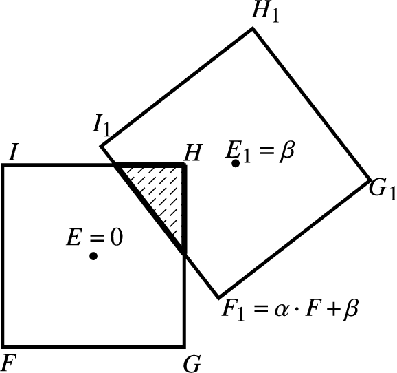
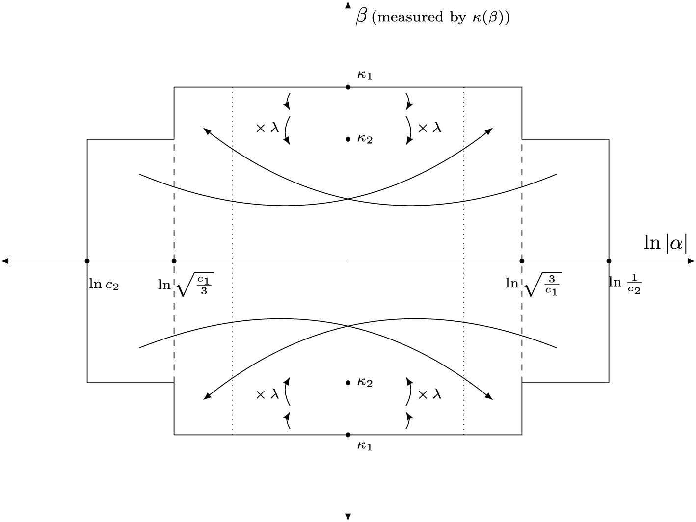
1 Introduction
The theory of regular Cantor sets in the real line has played a central role in the study of dynamical systems, especially in relation to their uniform hyperbolicity, that is, the existence of a decomposition of the tangent bundle over the non-wandering set of some map into two sub-bundles, one uniformly contracted by the action of the tangent map and the other one uniformly expanded. A diffeomorphism is called Axiom A when, additionally, the periodic points are dense in its non-wandering set. Some of the first results from the theory were the works of Newhouse [Reference Newhouse11–Reference Newhouse13], where he showed that there is an open set U in the space of
 $C^2$
diffeomorphisms of a compact surface (
 $\mathit {Diff}^2(\mathcal {M}^2)$
) such that any diffeomorphism in U is not hyperbolic. More than that, he observed that diffeomorphisms exhibiting a homoclinic tangency belonged to the closure of the set U.
In those works, he associated the presence of a tangency between the stable and unstable manifolds of a horseshoe, that is, a homoclinic tangency, to an intersection between two Cantor sets (constructed from the dynamical system). Then, an open set in
 $\mathit {Diff}^2(\mathcal {M}^2)$
with persistence of homoclinic tangencies was constructed via a pair of Cantor sets
 $(K_1, K_2)$
that had stable intersections, that is,
 $\tilde {K}_1\cap \tilde {K}_2$
was non-empty for any small perturbations
 $\tilde {K}_1$
and
 $\tilde {K}_2$
of
 $K_1$
and
 $K_2 $
. To construct such a pair, he developed a sufficient criterion for this phenomenon: the gap lemma. Precisely, he defined
 $\tau (K)$
, the thickness of a Cantor set K, which is a positive real number associated to the geometry of the gaps of K, and showed that if the product
 $\tau (K_1) \cdot \tau (K_2)$
is larger than one for a pair of Cantor sets
 $K_1$
and
 $K_2$
, then the pair
 $(K_1,K_2+t)$
has stable intersection for certain values of t.
Similar results were obtained in other contexts, such as in the works of Palis and Viana on larger dimensions [Reference Palis and Viana16] and of Duarte [Reference Duarte6] on conservative systems. We are more interested however in the work of Buzzard [Reference Buzzard4], who found an open region in the space of automorphisms of
 $\mathbb {C}^2$
, that is, holomorphic diffeomorphisms, with persistent homoclinic tangencies. His strategy was very similar to the first work of Newhouse [Reference Newhouse11], where he constructed a ‘very thick’ horseshoe, such that the Cantor sets, this time living in the complex plane, associated to it would also be ‘very thick’. However, the concept of thickness does not have a simple extension to this complex setting and so the argument to guarantee intersections between the Cantor sets after a small perturbation is different. It is worth noticing that a version of the gap lemma for holomorphic Cantor sets was recently discovered, in 2018, by Biebler (see [Reference Biebler1]).
The objective of this paper is to present a criterion for stable intersection of Cantor sets that works for the Cantor sets derived from horseshoes appearing in automorphisms of
 $\mathbb {C}^2$
. We begin by defining conformal Cantor sets. These sets are, roughly speaking, the maximal invariant set of a
 $C^{1+\varepsilon }$
expanding map g defined on a subset of
 $\mathbb {R}^2$
(satisfying some properties, see §2.1 up to Definition 2.1 for details) with the key hypothesis being its derivative is conformal over the invariant set, that is, the Cantor set itself. Throughout this article, we will freely identify a conformal operator over
 $\mathbb {R}^2$
with the operator over
 $\mathbb {C}$
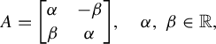
given by a multiplication by a complex number. Precisely, if
 $$ \begin{align*} A=\begin{bmatrix}\alpha &-\beta \\ \beta &\alpha\end{bmatrix}\!, \quad \alpha,\, \beta \in \mathbb{R},\end{align*} $$
we identify it with the operator over
 $\mathbb {C}$
given by the multiplication by
 $\alpha + \beta \cdot \mathrm {i}$
. Also, a map between two open sets of
 $\mathbb {C}^n$
is said to be
 $C^r$
, for some
 $r \in \mathbb{R}$
, if it is
 $C^r$
when seen as a map between two open subsets of
 $\mathbb{R}^{2n}$
.
We then proceed to show that this is the appropriate concept to study horseshoes appearing in automorphisms of
 $\mathbb {C}^2$
, which we call complex horseshoes. In this text, they are nothing more than totally disconnected non-trivial basic sets of saddle type (see §2.2 for the corresponding definitions). It is necessary to observe that this nomenclature already appears in the literature and was introduced in the thesis of Oberste-Vorth [Reference Oberste-Vorth14] as a complex version of the Smale horseshoe. These complex horseshoes are a particular case of the concept of a horseshoe presented in this text. Also, the work of Oberste-Vorth shows the existence of complex horseshoes whenever there is a transversal homoclinic intersection for an automorphism of
 $\mathbb {C}^2$
, a fact that justifies our interest in these kinds of objects. The details regarding these objects are given in the second section of this paper, and its main theorem is copied as follows.
Theorem 1.1 (Theorem 2.5)
Let
 $\Lambda $
be a complex horseshoe for an automorphism
 $G \in \mathrm{Aut}(\mathbb {C}^2)$
and p be a periodic point in
 $\Lambda $
. Then, if
 $\varepsilon $
is sufficiently small, there are an open set
 $U \subset \mathbb {C} $
, an open set
 $V \subset W^u_\varepsilon (p)$
containing p, and a holomorphic parameterization
 $\pi : U \to V$
such that
 $\pi ^{-1}(V \cap \Lambda )$
is a conformal Cantor set in the complex plane.
In §3, we extend the recurrent compact criterion created by Moreira and Yoccoz in [Reference Moreira and Yoccoz10] to this type of Cantor set. Here we see the importance of the conformality of our sets. It allows us to construct limit geometries, which are, roughly speaking, approximations of the asymptotic shape of small pieces of the Cantor sets (see the beginning of §3.1 and Lemma 3.1). The set of all limit geometries (for a given Cantor set) is a compact set. Because of that, we can prove the recurrent compact criterion: if, for some pair of Cantor sets, we can find a compact set of relative affine configurations of limit geometries (see Definition 3.4) that is carried to its own interior by renormalization operators, that is, a recurrent compact set (see Definition 3.5), then the original pair of Cantor sets, after an affine transformation on one of its entries, has stable intersection.
The concept of stable intersection is very similar to that in the real line setting. We say that two Cantor sets K and
 $K'$
are close to each other when the maps defining them are close to each other and so are the connected pieces of their domains
 $G(a)$
and
 $G'(a)$
(see Definition 2.2 and the paragraph below it). Also, we define a configuration of a piece
 $G(a)$
as a
 $C^{1+\varepsilon }$
embedding
 $h: G(a) \to \mathbb {C}$
(see Definition 3.1). That way, given a pair of configurations (
 $h, \,h'$
), also referred to as a configuration pair or a relative positioning, we say it has stable intersections whenever, for any pair
 $(\tilde {h},\tilde {h}')$
close to (
 $h, \,h'$
) and any pair of Cantor sets
 $(\tilde {K},\tilde {K}')$
on a small neighborhood of
 $(K,\,K')$
, the intersection between
 $\tilde {h}(\tilde {K})$
and
 $\tilde {h}'(\tilde {K}')$
is non-empty (see §3.3 for the details). The main result of §3 is the following.
Theorem 1.2 (Theorem 3.12)
The following properties are true.
-
(1) Every recurrent compact set is contained in an immediately recurrent compact set.
-
(2) Given a recurrent compact set
 $\mathcal {L}$
(respectively immediately recurrent) for g,
$g'$
, for any
$(\tilde {g}, \tilde {g}')$
in a small neighborhood of
$(g,g') \in \Omega _{\Sigma } \times \Omega _{{\Sigma }'}$
, we can choose base points
$\tilde {c}_a \in \tilde {G}(a) \cap \tilde {K}$
and
$\tilde {c}_{a'} \in \tilde {G}(a') \cap \tilde {K}'$
respectively close to the pre-fixed
$c_a$
and
$c_{a'}$
, for all
$a \in \mathbb {A}$
and
$a' \in \mathbb {A'}$
, in a manner that
$\mathcal {L}$
is also a recurrent compact set for
$\tilde {g}$
and
$\tilde {g}'$
.
-
(3) Any relative configuration contained in a recurrent compact set has stable intersections.


It is important to observe that the work of Moreira and Yoccoz [Reference Moreira and Yoccoz10] was done to solve a conjecture of Palis: for generic pairs of Cantor sets in the real line
 $K_1$
and
 $K_2$
, the arithmetic difference between
 $K_1$
and
 $K_2$
,
 $K_1 - K_2$
, contains an interval or has Lebesgue measure zero. This conjecture was inspired by the work of Palis and Takens [Reference Palis and Takens15], where they proved a theorem that assured full density of hyperbolicity on a parameter family that generically unfolds a homoclinic tangency, provided that the Hausdorff dimension of the horseshoe is less than one. The recurrent compact criterion was one of the tools used by them to show that for generic pairs
 $K_1, \, K_2$
of Cantor sets whose sum of Hausdorff dimension is larger than one (if the sum of Hausdorff dimensions is less than one, the arithmetic difference
 $K_2-K_1$
has Hausdorff dimension less than one and so Lebesgue measure zero), there is a real number t such that
 $K_1$
and
 $K_2 + t$
have a stable intersection, which implies in particular that
 $K_2-K_1$
contains an interval around t.
Another motivation is the work of Dujardin and Lyubich [Reference Dujardin and Lyubich8], who showed that homoclinic tangencies are the main obstruction to weak
 $J^{*}$
-stability, a concept related to the absence of bifurcation on the type of periodic points (saddle, node, repeller, or indifferent). Results regarding families unfolding homoclinic tangencies are also possible with our techniques and will appear in another paper. The general dichotomy that the arithmetic difference of conformal Cantor sets on the complex plane generically has zero measure or contains an open set is under development in a joint work with Zamudio, who has developed the scale recurrence lemma [Reference Zamudio20], another important tool.
We end this paper in §4 by showing that Buzzard’s construction can be interpreted as a case of stable intersection of conformal Cantor sets derived from the recurrent compact criterion. We also give (non-optimal) estimates on how ‘thick’ the Cantor sets have to be. The main result of it is the following.
Theorem 1.3 (Theorem 4.1)
There is
 $\delta $
sufficiently small for which the pair of Cantor sets
 $(K,K)$
defined for Buzzard’s example has a recurrent compact set of affine configurations of limit geometries
 $\mathcal {L}$
such that
 $[\mathrm{Id},\mathrm{Id}] \in \mathcal {L}$
.
We did not aim for an optimal estimate on
 $\delta $
because that would complicate the argument and it may be better to work with other constructions. It may also be possible to use the recurrent compact criterion to construct other families of Cantor sets (considering Buzzard’s example as a family parameterized by
 $\delta $
, the space between the pieces) that would have stable intersection with any other sufficiently general Cantor set. This could be useful when tackling the question whether automorphisms displaying a homoclinic tangency lie in the closure of the open set of persistent tangencies, as shown by Newhouse in [Reference Newhouse13] for the real case.
Before the main part of the text, we fix some notation. The space of affine complex transformations is denoted by
 $\textrm{Aff}(\mathbb {C}):= \{A: \mathbb {C} \to \mathbb {C};\,A(z)=\alpha \cdot z +\beta , \, \alpha \in \mathbb {C}^*,\,\beta \in \mathbb {C}\}$
and the space of affine transformations over
 $\mathbb {R}^2$
is denoted by
 $\textrm{Aff}(\mathbb {R}^2):=\{A: \mathbb {R}^2 \to \mathbb {R}^2;\,A(z)=DA\cdot z +\beta , \, DA \in GL(\mathbb {R}^2),\,\beta \in \mathbb {R}^2 \} $
. The
 $\delta $
-neighborhood of a set
 $X \subset \mathbb {R}^2$
is denoted by
 $V_{\delta }(X): = \{z \in \mathbb {R}^2;\text { there exists } x \in X,\,|z-x|<\delta \}$
. The norm of any vector will be denoted by
 $|\,\cdot \,|$
and the vector space where it lives will be clear by the context. The uniform norm of functions
 $f: X \to Y$
, where X and Y are subsets of normed vector spaces, will be denoted by
 $\lVert f \rVert := \mathop {\mathrm {sup}}\nolimits _{x \in X} \lvert f(x) \rvert $
. For
 $k \in \mathbb {R}$
greater than
 $1$
, we denote by
 $\lfloor k \rfloor $
the greatest integer smaller than or equal to k and if
 $k \notin \mathbb {N}$
, we denote the
 $C^{k}$
norm of a function
 $f: X \to \mathbb {R}^2$
by
 $$ \begin{align*} \lVert f \rVert_{C^{k}} = \lVert f \rVert_{C^{\lfloor k \rfloor}} + \mathop{\mathrm{sup}}\limits_{x \neq y \in X}{\frac{\lvert D^{\lfloor k \rfloor}f(x) - D^{\lfloor k \rfloor}f(y) \rvert}{\lvert x - y \rvert^{k - \lfloor k \rfloor}}}. \end{align*} $$
Whenever we say a function is
 $C^{1+\varepsilon }$
, we mean that
 $\varepsilon $
is a real number such that
 $0 < \varepsilon < 1$
.
2 Dynamically defined conformal Cantor sets in the complex plane and their relation to horseshoes
In this section, we define conformal (or, equivalently, asymptotically holomorphic) Cantor sets and establish some basic properties as well as their relation to complex horseshoes, which are important invariant hyperbolic sets of automorphisms of
 $\mathbb {C}^2$
.
2.1 Dynamically defined conformal Cantor sets
A regular (also called dynamically defined) Cantor set in
 $\mathbb {C}$
is given by the following data.
-
• A finite set
$\mathbb {A}$
of letters and a set
$B \subset \mathbb {A} \times \mathbb {A} $
of admissible pairs. -
• For each
$a\in \mathbb {A}$
, a compact connected set
$G(a)\subset \mathbb {C}$
. -
• A
$C^{1+\varepsilon }$
map
$g: V \to \mathbb {C}$
defined on an open neighborhood V of
$\bigsqcup _{a\in \mathbb {A}}G(a)$
.


These data must verify the following assumptions.
-
• The sets
$G(a)$
,
$a \in \mathbb {A}$
, are pairwise disjoint. -
•
$(a,b)\in B $
implies
$G(b) \subset g(G(a))$
, otherwise
$G(b) \cap g(G(a)) = \emptyset $
. -
• For each
$a \in \mathbb {A}$
, the restriction
$g|_{G(a)}$
can be extended to a
$C^{1+\varepsilon }$
embedding (with
$C^{1+\varepsilon }$
inverse) from an open neighborhood of
$G(a)$
onto its image such that
$m(Dg)> \mu $
for some constant
$\mu> 1$
, where
$m(A) := {\inf _{v\in \mathbb {R}^2 \equiv \mathbb {C}}{\lvert Av \rvert }/{\lvert v \rvert }}$
, A being a linear operator on
$\mathbb {R}^2$
. -
• The subshift
$(\Sigma , \sigma )$
induced by B, called the type of the Cantor set
$$ \begin{align*} \Sigma=\{ \underline{a}= (a_0, a_1, a_2, \ldots ) \in \mathbb{A}^{\mathbb{N}}:(a_i,a_{i+1}) \in B, \text{ for all } i \geq 0\} \text{, } \end{align*} $$
$\sigma (a_0,a_1,a_2, \ldots ) = (a_1,a_2,a_3, \ldots )$
is topologically mixing.


Once we have all these data, we can define a Cantor set (that is, a totally disconnected, perfect compact set) on the complex plane:
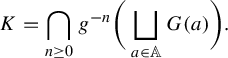 $$ \begin{align*} K=\bigcap_{n \geq 0} g^{-n}\bigg( \bigsqcup_{a \in \mathbb{A}} G(a) \bigg). \end{align*} $$
We will usually write only K to represent all the data that define a particular dynamically defined Cantor set. Of course, the compact set K can be described in multiple ways as a Cantor set constructed with the objects above, but whenever we say that K is a Cantor set, we assume that one particular set of data as above is fixed. In this spirit, we may represent the Cantor set K by the map g that defines it as described above, because all the data can be inferred if we know g. Also, when we are working with two Cantor sets
 $K \text { and }K'$
, we denote all the defining data related to the second accordingly. In other words,
 $K'$
is given by a finite set
 $\mathbb {A}'$
, a set
 $B'$
of admissible pairs, a function
 $g'$
defined on a neighborhood of compact connected sets
 $G(a')$
, etc. We use the same convention for future objects that will be defined related to Cantor sets, such as limit geometries and configurations.
Definition 2.1 (Conformal regular Cantor set)
We say that a regular Cantor set is conformal whenever the map g is conformal at the Cantor set K, that is,
 $\text { for all } x \in K$
,
 $Dg(x):\mathbb {C} \equiv \mathbb {R}^2 \to \mathbb {C} \equiv \mathbb {R}^2$
is a linear transformation that preserves angles or, equivalently, a multiplication by a non-zero complex number.
There is a natural topological conjugation between the dynamical systems
 $(K,g|_K)$
and
 $(\Sigma , \sigma )$
, the subshift
 $\Sigma $
induced by B. It is given by a homeomorphism
 $H: K \to \Sigma $
that carries each point
 $x \in K$
to the sequence
 $\{a_n\}_{n \geq 0}$
that satisfies
 $g^n(x) \in G(a_n)$
.
Associated to a Cantor set K, we define the sets
 $$ \begin{align*} \Sigma^{fin} & = \{(a_0, \ldots ,a_n): (a_i,a_{i+1}) \in B \quad \text{ for all } i , 0 \leq i < n \},\\ \Sigma^- & = \{(\ldots, a_{-n}, a_{-n+1},\ldots,a_{-1},a_0): (a_{i-1},a_i) \in B \quad \text{ for all } i \leq 0\}. \end{align*} $$
Given
 $\underline {a}=(a_0, \ldots , a_n)$
,
 $\underline {b}=(b_0, \ldots , b_m)$
,
 $\underline {\theta }^1=(\ldots ,\theta ^1_{-2},\theta ^1_{-1},\theta ^1_{0})$
, and
 $\underline {\theta }^2 = (\ldots ,\theta ^2_{-2}, \theta ^2_{-1},\theta ^2_{0})$
, we denote:
-
• if
$a_n=b_0$
,
$\underline {ab}=(a_0, \ldots ,a_{n}, b_1, \ldots , b_m)$
; -
• if
$\theta ^1_0=a_0$
,
$\underline {\theta ^1a} = (\ldots , \theta ^1_{-2},\theta ^1_{-1}, a_0, \ldots , a_n )$
; -
• if
$\underline {\theta }^1 \neq \underline {\theta }^2$
and
$\theta ^1 _0 = \theta ^2_ 0$
,
$\underline {\theta }^1 \wedge \underline {\theta }^2=(\theta _{-j}, \theta _{-j+1}, \ldots , \theta _0)$
, in which
$\theta _{-i} =\theta ^1 _{-i}= \theta ^2 _{-i} $
for all
$i=0, \ldots , j $
and
$\theta ^1_{-j-1} \neq \theta ^2_{-j-1}$
.


For
 $\underline {a}=(a_0, a_1, \ldots , a_n) \in \Sigma ^{fin}$
, we say that it has size n and define
 $$ \begin{align*} G(\underline{a})= \bigg\{x \in \bigsqcup_{a \in \mathbb{A}} G(a) , \; g^j(x) \in G(a_j), \;j=0,1,\ldots, n \bigg\} \end{align*} $$
and the function
 $f_{\underline {a}}: G(a_n) \to G(\underline {a})$
by
 $$ \begin{align*} f_{\underline{a}} = g|^{-1}_{G(a_0)} \circ g|^{-1}_{G(a_1)} \circ \cdots \circ (g|^{-1}_{G(a_{n-1})})|_{G(a_n)}. \end{align*} $$
Notice that
 $f_{(a_i,a_{i+1})} = g|^{-1}_{G(a_{i})}$
.
In our definition, we did not require the pieces
 $G(a)$
to have non-empty interior. However, if this is not the case, it is easy to see that we can choose
 $\delta $
sufficiently small such that the sets
 $G^*(a)= V_\delta (G(a))$
satisfy the following.
-
(i)
$G^*(a)$
is open and connected. -
(ii)
$G(a) \subset G^*(a)$
and
$g|_{G(a)}$
can be extended to an open neighborhood of
$\overline {G^*(a)}$
, such that it is a
$C^{1+\varepsilon }$
embedding (with
$C^{1+\varepsilon }$
inverse) from this neighborhood to its image and
$m(Dg)> \mu $
. -
(iii) The sets
$\overline {G^*(a)}$
,
$a \in \mathbb {A}$
, are pairwise disjoint. -
(iv)
$(a,b) \in B$
implies
$\overline {G^*(b)}\subset g(G^*(a))$
, and
$(a,b) \notin B$
implies
$\overline {G^*(b)}\cap \overline {g(G^*(a))} \,{=}\, \emptyset $
.


With this notation, we have the following lemma.
Lemma 2.1 Let K be a dynamically defined Cantor set and
 $G^*(a)$
the sets defined above. Let
 $G^*(\underline {a})$
be defined in the same way as
 $G(\underline {a})$
. There exist a constant
 $C> 0$
such that
 $$ \begin{align*} {\mathrm{diam}}(G^*(\underline{a})) < C\mu^{-n}, \end{align*} $$
where
 $\mu> 1$
is such that
 $m(Dg)> \mu $
in
 $\sqcup _{a \in \mathbb {A}}G^*(a)$
.
Proof. The proof is essentially the same as in [Reference Zamudio20]. For
 $\underline {a}\in \Sigma ^{fin}$
, let
 $d_{\underline {a}}$
be the metric
 $$ \begin{align*} d_{\underline{a}}(x,y) = \inf_{\alpha} l(\alpha), \end{align*} $$
where
 $\alpha $
runs through all smooth curves inside
 $G^*(\underline {a})$
that connect x to y and
 $l(\alpha )$
denotes the lengths of such curves. Because g sends
 $G^*(a_0,a_1,\ldots ,a_n)$
diffeomorphically onto
 $G^*(a_1,\ldots ,a_n)$
and
 $m(Dg)> \mu $
, then
 $$ \begin{align*} d_{(a_1, \ldots, a_n)}(g(x),g(y)) \geq \mu \cdot d_{a_0, \ldots, a_n}(x,y) \end{align*} $$
for all
 $x,y \in G^* (a_0, \ldots a_n)$
. Therefore,
 $$ \begin{align*} \text{diam}_{(a_0, \ldots a_n)}(G^* (a_0, \ldots a_n)) \leq \mu ^{-1} \cdot \text{diam}_{(a_1, \ldots a_n)}(G^* (a_1, \ldots a_n)), \end{align*} $$
where
 $\text {diam}_{\underline {a}}$
is the diameter with respect to
 $d_{\underline {a}}$
. We conclude that, by induction,
 $$ \begin{align*} \text{diam}(G^*(\underline{a}))\leq \text{diam}_{\underline{a}}(G^*(\underline{a})) \leq \mu^{-n} \cdot \text{diam}_{{a}_n}(G^*({a}_n)). \end{align*} $$
Taking any C larger than
 $\max _{a \in \mathbb {A}} \text {diam}(G^*(a))$
yields the result.
As a consequence of this lemma, we can see that
 $$ \begin{align*} K=\bigcap_{n \geq 0}g^{-n}\bigg(\bigsqcup_{a \in \mathbb{A}}G^*(a)\bigg), \end{align*} $$
because
 $G(\underline {a})\subset G^*(\underline {a})$
and
 $\text {diam}(G^*(\underline {a})) \rightarrow 0$
.
In this manner, the sets
 $G(a)$
can be substituted by the sets
 $\overline {G^*(a)}$
in the definition of K. So in what follows, additional to the properties in the definition of Cantor sets, we suppose that
 $G(a)=\overline {\mathring {(G(a))}}$
and that g can always be extended to a neighborhood
 $V_a$
of
 $G(a)$
such that it is a
 $C^{1+\varepsilon }$
embedding (with
 $C^{1+\varepsilon }$
inverse) and
 $m(Dg)> \mu $
over
 $V_a$
, which by Lemma 2.1 implies that
 $\text {diam}(G(\underline {a}))< C \mu ^{-n}$
, if
 $\underline {a} = (a_0, \ldots a_n)$
. The most important examples of conformal Cantor sets come from intersections between compact parts of stable and unstable manifolds of periodic points and basic sets of saddle type of an automorphism of
 $\mathbb {C}^2$
and, as we will see, we can construct them from sets
 $G(a)$
with these properties already.
Finally, we have the following definition.
Definition 2.2 (The space
$\Omega _{\Sigma }$
)

The set of all conformal regular Cantor sets K with the type
 $\Sigma $
is defined as the set of all conformal Cantor sets described as above, whose set of data includes an alphabet
 $\mathbb {A}$
and the set B of admissible pairs used in the construction of
 $\Sigma $
. We denote it by
 $\Omega _{\Sigma }$
.
We are also interested in how limit geometries vary related to the map g in the case where it has higher regularity. Thus, given any real number
 $r> 1$
, we define
 $\Omega _{\Sigma }^r$
in the same way as above only requiring the maps g to be
 $C^r$
for this fixed r.
These spaces will be seen as topological spaces. The topology on
 $\Omega _{\Sigma }^r$
is generated by a basis of neighborhoods
 $U_{K,\delta } \subset \Omega _{\Sigma }, \, K \in \Omega _{\Sigma }, \, \delta> 0 $
, where
 $U_{K,\delta }$
is the set of all conformal regular Cantor sets
 $K'$
given by
 $g': V' \to \mathbb {C}, \, V' \supset \bigsqcup _{a \in \mathbb {A}} G'(a)$
such that
 $G(a) \subset V_{\delta }(G'(a))$
,
 $G'(a) \subset V_{\delta }(G(a))$
(that is, the pieces are close in the Hausdorff topology), and the restrictions of
 $g'$
and g to
 $V \cap V'$
are
 $\delta $
close in the
 $C^{r}$
metric. Because
 $\Omega _{\Sigma } = \cup _{r>1}\Omega _{\Sigma }^r$
, we equip it with the inductive limit topology, that is, the finest topology such that the inclusions
 $\Omega ^r_{\Sigma }\subset \Omega _{\Sigma }$
are continuous maps. See [Reference Dugundji7] for more details.
2.2 Semi-invariant foliations in a neighborhood of a horseshoe
As pointed out in §1, complex horseshoes are important hyperbolic invariant sets appearing in automorphisms of
 $\mathbb {C}^2$
, mainly because they are present whenever there is a transversal homoclinic intersection, as shown by [Reference Oberste-Vorth14]. We now give a quick review of these concepts and explain how to construct semi-invariant foliations on the neighborhood of a complex horseshoe.
Given a diffeomorphism
 $F: M \to M$
of class
 $C^k$
on a Riemannian manifold M, we say that a compact invariant set
 $\Lambda \subset M$
(by invariant, we mean that
 $F(\Lambda )=\Lambda $
) is hyperbolic when there are constants
 $C>0$
,
 $\lambda < 1 $
, and a continuous splitting
 $TM| \Lambda = E^s \oplus E^u$
such that:
-
• it is invariant, that is,
$DF_x(E^s(x)) = E^s(F(x))$
and
$DF_x(E^u(x)) = E^u(F(x))$
; -
• and for any
$x \in \Lambda $
,
$v^s \in E^s(x)$
, and
$v^u \in E^u(x)$
, we have
$$ \begin{align*}|DF^j(v^s)|_{F^j(x)}< C\lambda^j |v^s|_x \quad \text{and}\quad |DF^{-j}(v^u)|_{F^{-j}(x)} < C\lambda^j |v^u|_x, \quad \text{for all } j \in \mathbb{N},\end{align*} $$


where
 $|\cdot |_x$
is the norm on
 $T_xM$
associated to the Riemannian metric, which we will call d. The bundle
 $E^s$
above is called the stable sub-bundle and the bundle
 $E^u$
is called the unstable sub-bundle.
Hyperbolic sets are useful because we have a good control on the sets of points that asymptotically converge to them. For any
 $\varepsilon>0$
and any point x in a hyperbolic set
 $\Lambda $
, we define the stable manifold and the local stable manifold by
 $$ \begin{align*} W^s(x) =\{y \in M,\lim_{n \rightarrow +\infty}d(F^n(y),F^n(x))=0\} \end{align*} $$
and
 $$ \begin{align*} W^s_{\varepsilon}(x) =\{y \in M,d(F^n(y),F^n(x))< \varepsilon, \text{ for all } n \geq 0\}, \end{align*} $$
respectively. It is a classical result that
 $W^s(x)$
is a
 $C^k$
-immersed manifold and, if
 $\varepsilon $
is sufficiently small, independently of x,
 $W^s_\varepsilon (x)$
is a
 $C^k$
-embedded disk tangent to
 $E^s(x)$
. The same results remain true for the unstable versions of the objects above, defined by considering backwards iterates
 $F^{-n}$
instead of the forwards ones above. We denote the unstable manifold and the local unstable manifold by
 $W^u(x)$
and
 $W^u_\varepsilon (x)$
, respectively. Also, it is important to observe that they vary continuously with
 $x \in \Lambda $
in the
 $C^k$
topology and are invariant in the sense that
 $F(W^{s,u}(x))=W^{s,u}(F(x))$
.
In the special case that F is an automorphism of
 $\mathbb {C}^2$
, that is, a holomorphic diffeomorphism of
 $\mathbb {C}^2$
, the manifolds above are complex manifolds. Also, the sub-bundles
 $E^s$
and
 $E^u$
are such that
 $E^{s,u}(x)$
is a complex linear subspace of
 $T_x\mathbb {C}^2 \equiv \mathbb {C}^2$
.
Going back to the general setting, we say that the hyperbolic set
 $\Lambda $
on M has a local product structure if there exists
 $\varepsilon> 0$
such that, for any
 $x,y \in \Lambda $
sufficiently close,
 $W^s_{\varepsilon }(x) \cap W^u_{\varepsilon }(y)$
consists of a single point z that also belongs to
 $\Lambda $
. This structure makes the neighborhood (in
 $\Lambda $
) of a point
 $x \in \Lambda $
homeomorphic to the product
 $ (W^s_{\varepsilon }(x) \cap \Lambda ) \times (W^u_{\varepsilon }(x) \cap \Lambda ) $
. Also, this condition is equivalent to
 $\Lambda $
being locally maximal, that is, there is an open set U (
 $\Lambda \subset U$
) such that
 $\Lambda =\bigcap _{n \in \mathbb {Z}} F^n(U)$
. We say that the hyperbolic set is transitive when there is an
 $x \in \Lambda $
such that
 $\{F^n(x), n \in \mathbb {Z}\}$
is dense in
 $\Lambda $
. A hyperbolic set with these two properties is called a basic set.
A horseshoe is a particular type of basic set. It has the additional properties:
-
• it is infinite;
-
• it is of saddle-type, that is, the bundles
$E^s$
and
$E^u$
are non-trivial; and -
• it is totally disconnected.


The dynamics of F over a horseshoe
 $\Lambda $
is conjugated to a Markov shift of finite type, similarly to the Smale horseshoe, which is conjugated to
 $\{0,1\}^{\mathbb {Z}}$
. The last hypothesis implies that, in particular, a horseshoe is a zero-dimensional set and so it is topologically a Cantor set. We observe that, because of Smale’s Spectral Decomposition Theorem, any horseshoe for a diffeomorphism F can be decomposed into finitely many components, each of them being topologically mixing for some iterate
 $F^m$
of F. Thus, from now on, we assume that all horseshoes are topologically mixing.
Horseshoes appearing in automorphisms of
 $\mathbb {C}^2$
will be called complex horseshoes in this paper. As pointed out in §1, this nomenclature does not conflict with that used by Oberste-Vorth in [Reference Oberste-Vorth14], that is, the horseshoes constructed there are horseshoes in our sense. Another important example, to which we will refer many times in this paper, is the one constructed by Buzzard in [Reference Buzzard4] to study Newhouse regions in
 $\mathrm{Aut}(\mathbb {C}^2$
). The objective of this section is to show that a complex horseshoe is, locally, close to the product of two conformal Cantor sets, as defined in the previous subsection. To do so, we will first need to construct stable and unstable foliations in some neighborhood of it, which is the other objective of this subsection.
This is done in the next theorem, which is just a small adaptation of a theorem of Pixton [Reference Pixton17] used by Buzzard in [Reference Buzzard4]. The only difference is that we require the foliations to be
 $C^{1+\varepsilon }$
instead of just
 $C^1$
. However, before stating it, some remarks. For a foliation
 $\mathcal {F}$
, we will denote the leaf though a point p in its domain (which is an open set) by
 $\mathcal {L}(p)$
, and we will denote the stable and unstable foliations by
 $\mathcal {F}^{\kern1pt s}$
and
 $\mathcal{F}^{\kern1pt u}$
, respectively. In the statement, we will deal only with the unstable foliation, but the analogous result for the stable version can be done by exchanging G with
 $G^{-1}$
and
 $E^s$
with
 $E^u$
. The norm
 $\Vert DG|_{E^s,E^u}\Vert $
is equal to
 $\mathop {\mathrm {sup}}\nolimits _{x \in \Lambda } |DG|_{E^s(x),E^u(x)}| $
and this last norm is the one coming from the Riemannian metric of choice that we fix on
 $\mathbb {C}^2$
. Finally, the whole concept of a horseshoe works for local diffeomorphisms, or injective holomorphisms as follows.
Theorem 2.2 Let
 $U \subset \mathbb {C}^2$
. Let
 $\Lambda \subseteq U $
be a horseshoe for an injective holomorphism
 $G_0: U \to M$
, with
 $\Lambda ={\bigcap _{n\in \mathbb {Z}}G_0^n(U)}$
, and let
 $E^s \oplus E^u $
be the associated splitting of
 $T_{\Lambda }\mathbb {C}^2$
.
Suppose that
 $\Vert DG_0|_{E^s}\Vert \cdot \Vert DG_0^{-1}|_{E^u}\Vert \cdot \Vert DG_0^{-1} |_{E^s}\Vert ^{1+\varepsilon } < 1$
.
Then, there is a compact set L and
 $\delta>0$
such that for any holomorphism
 $G : U \to \mathbb {C}^2$
with
 $\Vert G-G_0\Vert <\delta $
, we can construct a
 $C^{1+\varepsilon }$
foliation
 $\mathcal {F}_G ^{\kern1pt u} $
defined on a open set
 $V\subset U$
such that:
-
• the horseshoe
$\Lambda _G = {\bigcap _{n \in \mathbb {Z}}G^n(U)}$
satisfies
$\Lambda _G \subset {\mathrm{int}}\, L \subset L \subset \mathcal {F}_G ^u $
; -
• if
$p \in \Lambda _G $
, then the leaf
$\mathcal {L}^u_G(p)$
agrees with
$W^u_{\textrm {loc}}(p)$
; -
• if
$p\in G^{-1}(L)\cap L$
, then
$G(\mathcal {L}^u_G (p) ) \supseteq \mathcal {L}^u_G (G(p))$
, that is, it is semi-invariant; -
• the tangent space
$T_p\mathcal {L}^u_G(p)$
varies
$C^{1+\varepsilon }$
with p and continuously with G; -
• the association
$G \to \mathcal{F}^{\kern1pt u}_G$
is continuous on the
$C^{1+\varepsilon }$
topology.


The proof of this theorem is provided in Appendix A. It contains a brief review of the argument by Pixton and then proceeds to the small changes necessary for our context.
Remark 2.3. The condition
 $\Vert DG_0|_{E^s}\Vert \cdot \Vert DG_0^{-1}|_{E^u}\Vert \cdot \Vert DG_0^{-1} |_{E^s}\Vert ^{1+\varepsilon } < 1$
is automatically satisfied, for
 $\varepsilon $
sufficiently small, for the horseshoe of Buzzard’s example (see Example 2.7). For general complex horseshoes, we cannot guarantee it. Nevertheless, the condition can be weakened to a pointwise one so that the theorem is still true. In fact, checking the proof presented in the appendix, including the particular version of the
 $C^r$
section theorem, we see that it is sufficient that
 $$ \begin{align*}\lvert DG_0|_{E^s(x)} \rvert \cdot \lvert DG_0^{-1}|_{E^u(x)} \rvert \cdot \lvert DG_0^{-1}|_{E^s(G_0(x))} \rvert^{1+\varepsilon}< C < 1 \end{align*} $$
for every
 $x \in \Lambda $
, where
 $C < 1$
is a constant uniform for all x. Observe that because
 $E^s(x)$
and
 $E^u(x)$
are complex lines in
 $\mathbb {C}^2$
and G is holomorphic, then
 $\lvert DG_0^{-1}|_{E^s(G_0(x))} \rvert = \lvert DG_0|_{E^s(x)} \rvert ^{-1}$
, and hence this condition can be simplified to
 $\Vert DG_0|_{E^s}\Vert ^{-\varepsilon }\cdot \Vert DG_0^{-1}|_{E^u}\Vert < 1$
.
Remember that whenever we have a hyperbolic set
 $\Lambda $
, there is an adapted metric
 $\Vert \,\cdot \,\Vert '$
such that the constant C in the definition of the hyperbolic set is equal to
 $1$
. In this metric, the condition
 $\Vert DG_0|_{E^s}\Vert ^{-\varepsilon }\cdot \Vert DG_0^{-1}|_{E^u}\Vert < 1$
will be automatically satisfied, for some
 $\varepsilon $
sufficiently small, with
 $\Vert \cdot \Vert '$
instead of
 $\Vert \cdot \Vert $
. Because such metrics are uniformly equivalent in a compact set containing both the foliations above, it follows that close to a complex horseshoe, we can always construct stable and unstable foliations with the properties listed in Theorem 2.2.
Remark 2.4. Each leaf of the foliation obtained in Theorem 2.2 can be chosen to be a holomorphic curve. This only depends on being able to consider the foliation
 $\mathcal {F}^1$
(see the proof in Appendix A) consisting of leaves that are holomorphic curves. The local construction of
 $\mathcal {F}^1$
in [Reference Pixton17] involves only an isotopy and a bump function applied to create disk families along compact (and possibly very small) parts of
 $W^s$
. Checking the details in the original, we observe that such construction can be done in a way that makes those disk families be holomorphic embedded curves. This is mentioned in [Reference Buzzard4]; see the appendix of [Reference Buzzard3] for further details.
2.3 Conformal Cantor sets locally describe horseshoes
To end this section, we show that a horseshoe is, locally, close to the product of two conformal Cantor sets. Having in mind the local product structure, this fact is a consequence of the following theorem.
Theorem 2.5 Let
 $\Lambda $
be a complex horseshoe for an automorphism
 $G \in \mathrm{Aut}(\mathbb {C}^2)$
and p be a periodic point in
 $\Lambda $
. Then, if
 $\varepsilon $
is sufficiently small, there are an open set
 $U \subset \mathbb {C} $
, an open set
 $V \subset W^u_\varepsilon (p)$
containing p, and a holomorphic parameterization
 $\pi : U \to V$
such that
 $\pi ^{-1}(V \cap \Lambda )$
is a conformal Cantor set in the complex plane.
Of course an analogous version is true for the stable manifold. The main ingredient is the following lemma.
Lemma 2.6 Let
 $\Lambda _G$
be a complex horseshoe for an automorphism
 $G \in \mathrm{Aut}(\mathbb {C}^2)$
together with its unstable foliation
 $\mathcal{F}^{\kern1pt u}_G$
. Additionally, let
 $N_1$
and
 $N_2$
be two
 $C^{1+\varepsilon }$
transversal sections to
 $\mathcal{F}^{\kern1pt u}_G$
. Suppose that for some periodic point
 $p \in \Lambda _G$
, the tangent planes of
 $N_1$
and
 $N_2$
to the points of intersection
 $N_1 \cap \mathcal {L}^u_G(p) =q_1$
and respectively
 $N_2 \cap \mathcal {L}^u_G(p)=q_2$
are complex lines of
 $\mathbb {C}^2$
. Then the projection along unstable leaves
 $\Pi _u : N_1 \to N_2$
is a
 $C^{1+\varepsilon }$
map conformal at
 $q_1$
.
Proof. Observe that, because
 $p \in \Lambda _G$
, every backwards iterate of the segment in
 $\mathcal {L}^u_G(p)$
that connects
 $q_1$
and
 $q_2$
stays on the domain of the foliation. So, for every
 $n \in \mathbb {N}$
, we can define small neighborhoods
 $ N_i^n \subset N_i$
of
 $q_i$
,
 $i=1,\,2$
, such that
 $G^{-n}(N^n_i)$
is also on the domain of the foliation. Furthermore, this restriction can be done in such manner that, because p is periodic and, by the inclination lemma,
 $G^{-n}(N^n_1)$
and
 $G^{-n}(N^n_2)$
are
 $\delta $
close to each other on the
 $C^1$
metric for every
 $n> n_\delta $
. Also, we can assume that their tangent directions at
 $q^n_i=G^{-n}(q_i)$
are bounded away from
 $T_{q^n_i}W^u_G$
,
 $i=1,\,2.$
Let
 $\Pi ^n_u : N^n_1 \to N^n_2$
be the projection along the unstable foliation.
There is a small neighborhood
 $\tilde {U}\subset \mathbb {C}^2$
of
 $q_1^n$
and
 $q_2^n$
, and a
 $C^{1+\varepsilon }$
map
 $f:\tilde {U} \to \mathbb {D}\times \mathbb {D}$
such that the unstable leaves are taken onto the horizontal levels
 $\mathbb {D} \times \{z\} \text {, } z \in \mathbb {D}$
, and
 $N^n_1$
and
 $N^n_2$
are taken onto graphs
 $(h_1(z), z)$
and
 $(h_2(z),z)$
of
 $C^{1+\varepsilon }$
embeddings
 $h_1 \text { and } h_2$
with the domain being a small disk
 $\mathbb {D}$
too. Under this identification,
 $\Pi ^n_u$
is a
 $C^{1+\varepsilon }$
map that carries
 $(h_1(z), z)$
to
 $(h_2(z),z)$
, and, because
 $G^{-n}(N^n_1)$
and
 $G^{-n}(N^n_2)$
are
 $\delta $
close to each other on the
 $C^1$
metric, has a derivative
 $\delta $
close to the identity.
Now, the projection along unstable foliations commute with G. Therefore,
 $\Pi _u = G^{n} \circ \Pi ^n_u \circ G^{-n}$
. Using the chain rule to calculate the derivative of
 $D\Pi _u$
at
 $q_1$
, we obtain an expression of the form
 $$ \begin{align*}A_1 \cdot A_2 \cdots A_n \cdot D\Pi_u^n \cdot B_n \cdots B_1,\end{align*} $$
where
 $B_i$
represents the restriction of
 $(DG)^{-1}$
to
 $T_{q_1^{i-1}}N_1^{i-1}$
and
 $A_i$
the restriction of
 $DG$
to
 $T_{q_2^i}N_2^i$
, for i from
 $1$
to n (
 $q_1^0=q_1$
and
 $N_1^0=N_1$
). However, all of these tangent spaces are, by induction, complex lines in
 $\mathbb {C}^2$
, so all the
 $A_i$
and
 $B_i$
are conformal. This way, the derivative of
 $\Pi _u$
is at most
 $\delta $
distant from being conformal. Making
 $\delta \rightarrow 0$
(or equivalently,
 $n \rightarrow \infty $
), we have the desired conformality.
The proof of Theorem 2.5 will be done using the Buzzard’s horseshoe [Reference Buzzard4] because it makes the comprehension easier and we will need this example later. For the general case, one need just to use Markov neighborhoods as in [Reference Pixton17], but the proof is easily deduced from the proof for this example. So now we proceed to a brief recapitulation of this example.
Example 2.7 (Buzzard)
Let
 $S(p;l) \subset \mathbb {C}$
denote the open square centered at p of sides parallel to the real and imaginary axis of side length equal to l. Consider the nine points set:
 $$ \begin{align*} P= \{x+yi \in \mathbb{C}; \, (x,y) \in \{-1,\,0,\,1\}^2 \} \end{align*} $$
and a positive real number
 $\delta <1$
. Define
 $c_0 = 1-\delta $
and
 $$ \begin{align*} K_0 := \displaystyle{\bigcup_{a \in P} \overline{S(a;c_0)}} \quad \text{and}\quad K_1 := K_0 \times K_0 \subset \mathbb{C}^2. \end{align*} $$
We identify each connected component of
 $K_1$
,
 $ S(a;c_0) \times S(b;c_0) $
, as the pair
 $(a,b) \in P^2$
.
Consider now some positive real number
 $c_1 \in (c_0 =1-\delta , {3c_0}/({2+c_0}) =({3-3\delta })/({3-\delta }))$
and the map
 $f: K_0 \to \mathbb {C}$
defined as
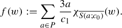 $$ \begin{align*} f(w):= \sum_{a \in P}\frac{3a}{c_1}\chi_{\overline{S(a;c_0)}}(w). \end{align*} $$
Notice that its image is composed of nine points as is P. Analogously, we can define
 $K_g := {\bigcup _{a \in P} \overline {S(3a/c_1;3)}} $
and define
 $$ \begin{align*} g(z):= \sum_{a \in P}-a\cdot\chi_{\overline{S({3a}/{c_1};3)}}(z). \end{align*} $$
Then, defining the maps:
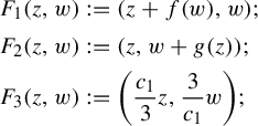 $$ \begin{align*} F_1(z,w)& : = (z+f(w), w);\\ F_2(z,w) &:=(z,w+g(z));\\ F_3(z,w) &:= \bigg(\frac{c_1}{3}z,\frac{3}{c_1}w\bigg); \end{align*} $$
and making
 $F:K_0 \times K_g \to \mathbb {C}^2 ,\; F:=F_3 \circ F_2 \circ F_1$
, we have that in a connected component
 $(a,b)$
of
 $\overline {K_1}$
,
 $$ \begin{align*} F(z,w) = \bigg(\frac{c_1}{3}z+b, \frac{3}{c_1}(w-b)\bigg). \end{align*} $$
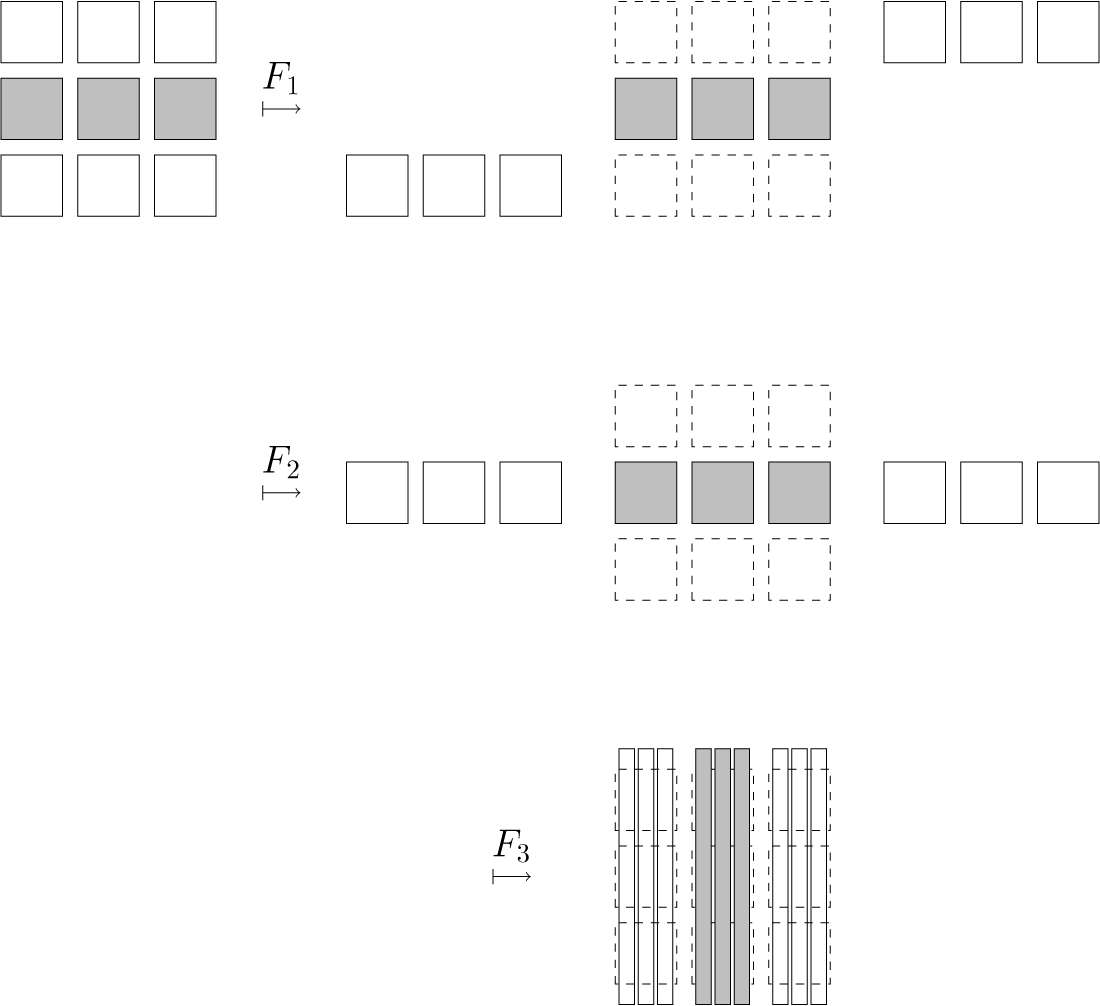
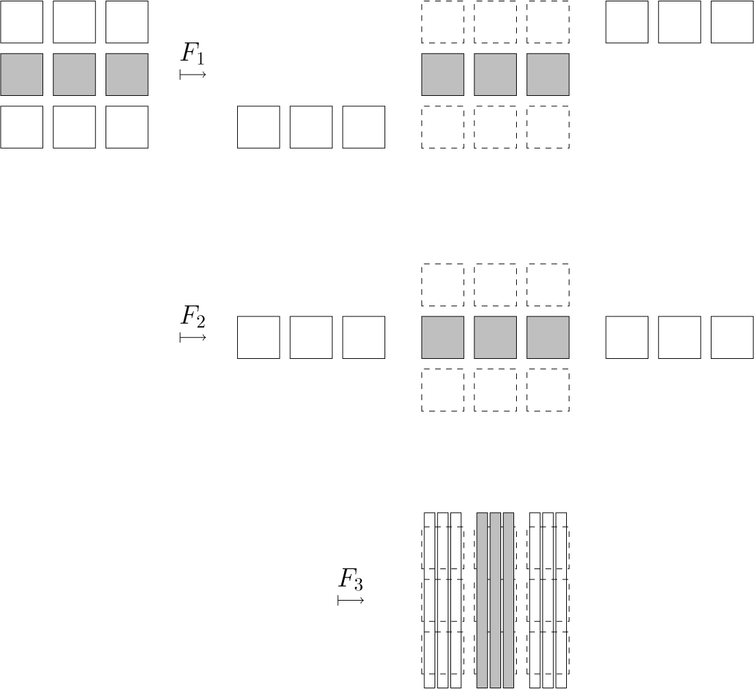
Figure 1 was presented in [Reference Buzzard4] and represents the map F.
A copy of the diagram in Buzzard’s paper explaining the behavior of F. The grid of nine squares actually represents
 $K_0 \times K_0$
and not the set
 $K_0$
itself. Each square represents a connected component of
 $K_0 \times K_0$
. Although there are
 $81$
of them, the diagram only presents nine, so it is a simplification of the exact situation. Moreover, each subset of
 $\mathbb {C}$
is represented by an interval.
The maximal invariant set of F over
 $K_1$
,
 $\Lambda = \bigcap _{n \in \mathbb {Z}} F^n(K_1) $
, is a hyperbolic set with
 $0$
as a fixed saddle point. It is easy to see that
 $W^u_{F,\text {loc}}((0,0)) := \{0\} \times \{ S(0; c_0) \} $
is the connected component that contains
 $(0,0)$
of the intersection between
 $W^u_F((0,0))$
and the connected component
 $(0,0)$
of
 $K_1$
. Also, the set
 $W^u_{F,\text {loc}}((0,0)) \cap \Lambda $
can be seen as a conformal Cantor set
 $K_F$
on the complex plane (in this case,
 $0 \times \mathbb {C}$
) given by the maps:
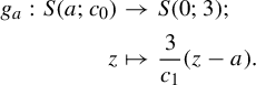 $$ \begin{align*} g_a: S(a;c_0) & \to S(0; 3);\\ z & \mapsto \frac{3}{c_1}(z-a). \end{align*} $$
Likewise, we can write
 $W^s_{F,\text {loc}}((0,0)) \cap \Lambda $
as the same Cantor set K. The condition
 $c_1 < ({3c_0}/({2+c_0}))$
is necessary for the image of each
 $g_a$
to cover the union of their domains.
Now we work with automorphisms of
 $\mathbb {C}^2$
that are sufficiently close to this model F. First, we use Runge’s theorem to approximate f and g on
 $\overline {K_0}$
and
 $\overline {K_g}$
respectively by polynomials
 $p_f$
and
 $p_g$
, obtaining a map
 $G_0 = F_3 \circ F^{\prime }_2 \circ F^{\prime }_1 \in \mathrm{Aut}(\mathbb {C}^2)$
, where
 $F^{\prime }_1(z,w) : = (z+p_f(w), w)$
and
 $F^{\prime }_2(z,w) :=(z,w+p_g(z))$
. Then, we fix
 $K' \subset \overline {K'} \subset \text {int}(K_1) $
such that, considering
 $\Lambda _G$
the maximal invariant set by G of the open set
 $K_1$
, it is contained in
 $K'$
whenever
 $\Vert G-G_0\Vert $
on
 $\overline {K_0 \times K_g}$
is sufficiently small. Furthermore, there is a fixed point
 $p_G$
that is the analytic continuation of the fixed point
 $(0,0)$
of F. Because
 $\Vert G-F\Vert $
is small, we can also show that the projection onto the first coordinate
 $\Pi : W^s(p_G; {\textrm {loc}}) \to S(0;3)$
is a biholomorphic map close to the identity, where
 $W^s(p_G; {\textrm {loc}})$
is the connected component that contains
 $p_G$
of
 $W^s(p_G) \cap U$
, where
 $U=S(0;3) \times S(0;({2+c_0})/{c_0})$
(notice it is a larger portion of the stable manifold than previously defined for F).
Observe that
 $G^{-1}(W^s(p_G; {\textrm {loc}})) \cap (S(0;({3}/{c_1})c_0)\times K_0 )$
is made of nine different connected components,
 $W_1, W_2, W_3, \ldots , W_9$
, each of them holomorphic curves close to being horizontal, because of the continuous dependence of the foliations on G (so, as long as f and g are well approximated by
 $p_f$
and
 $p_g$
and
 $\Vert G-G_0\Vert $
is sufficiently small). Consider now
 $V_i=G (W_i), \,i=1,2,\ldots ,9 $
. Notice that all the
 $V_i $
are disjoint subsets of
 $W^s(p_G; {\textrm {loc}})$
.
According to Theorem 2.2 and Remark 2.4,
 $\mathcal{F}^{\kern1pt u}_G$
can be defined whenever G is sufficiently close to F and we can consider its leaves to be holomorphic lines very close to the vertical lines. However, its domain may be only a small neighborhood of
 $\Lambda _G$
. We now show a way of constructing it that covers a large subset of U.
First, consider the foliation by vertical leaves
 $\{z\} \times S(0;3)$
defined for z on a small neighborhood of
 $\overline {S(0;3)}$
. For any real number
 $k>1 $
sufficiently close to
 $1$
, if G is sufficiently close to F, then
 $$ \begin{align*} S(a; k^{-1}c_1 ) &\times S(0;(2+c_0)k) \subset G(S(0;3) \times S(a; c_0 ))\\ &\quad\subset S(a; kc_1) \times S(0;3)\quad \text{for all } a \in P, \end{align*} $$
because the inclusions are true for F. Let
 $V_{-1}(a)= S(a; k^{-1}c_1 ) $
and
 $V_1(a)=S(a; kc_1 )$
as above. Observe that if k is sufficiently close to
 $1$
, for each
 $V_i$
, there is
 $a \in P$
such that
 $ \Pi (V_i) \subset V_{-1}(a)$
, again because it is true for F. Also, let
 $$ \begin{align*} V(a) = \Pi(G(S(0;3) \times S(a; c_0 )) \cap \{w=0\}) \subset \mathbb{C}. \end{align*} $$
Then
 $V_{-1}(a)\subset V(a) \subset V_{1}(a)$
. The image of the vertical foliation restricted to
 $S(0;3) \times S(a; c_0 )$
by G is a foliation of
 $G(S(0;3) \times S(a; c_0 ))$
described as
 $(u,v)\mapsto (u+\Psi _a(u,v), v)$
for
 $u \in V(a)$
and
 $v \in S(0;(2+c_0)k)$
(after an obvious shrinking), with
 $\Psi _a$
small in the
 $C^1$
metric as
 $\Vert G-F\Vert $
is small, once more, because it is true for F if we make
 $\Psi _a \equiv 0$
. Notice that
 $\Psi _a(u,v)$
is always holomorphic on v, which is equivalent to the fact that the leaves, given by
 $(u_0+\Psi _a(u_0,v),v)$
for
 $u_0$
fixed, are holomorphic curves.
For each
 $a \in P$
, fix
 $\lambda _a: \mathbb {C} \to [0,1]$
a bump function with support contained in
 $V(a)$
and such that
 $ V_{-1}(a)\subset \{\lambda _a(z) = 1\} \subset V(a)$
. It is easy to see that
 $\lambda _a$
with these properties can be chosen independently of G. We can now extend each of the foliations above to
 $V_{1}(a) \times S(0;2+c_0) $
by
 $$ \begin{align*} (u,v) \in V_{1}(a) \times S(0;2+c_0) \mapsto \begin{cases} (u+\lambda_a(u)\cdot\Psi_a(u,v), v) &\text{ for } u \in V(a), \\ (u,v) & \text{ for } u \in V_1(a) \setminus V(a),\end{cases} \end{align*} $$
which yields a foliation that is
 $C^{\infty }$
with holomorphic leaves (for each fixed
 $u_0$
). This foliation is
 $C^{\infty }$
but observe that it is not yet invariant in a neighborhood of the invariant set
 $\Lambda $
. The resultant invariant foliation
 $\mathcal {F}^{\kern1pt u}_{G}$
that is constructed from it, at the end of the argument, is only
 $C^{1+\varepsilon }$
in general. This resultant foliation is however still
 $C^{\infty }$
away from the set
 $\Lambda $
. By choosing
 $\lVert \Psi _a \rVert _{C^1}$
sufficiently small (relatively to
 $\Vert \lambda _a\Vert _{C^1}$
), which can be done by making G very close to F, we can guarantee that the map above is injective. To guarantee that it is surjective onto
 $V_{1}(a) \times S(0;2+c_0) $
, we observe that it is clearly surjective outside of
 $\operatorname {\mathrm {supp}} \lambda _a \times S(0;2+c_0) $
. Let
 $\tilde {V}(a)$
be a set homeomorphic to the closed ball such that
 $\operatorname {\mathrm {supp}} \lambda _a \subset \tilde {V}(a) \subset V(a)$
. For
 $u' \in \operatorname {\mathrm {supp}} \lambda _a$
and
 $v \in S(0; 2 + c_0)$
fixed, if
 $\lVert \Psi _a \rVert $
is sufficiently small, the map
 $$ \begin{align*} u \in \tilde{V}(a) & \to \mathbb{C} \\ u & \mapsto u' - \lambda_a(u)\cdot\Psi_a(u,v) \end{align*} $$
maps
 $\tilde {V}(a)$
inside itself, hence has a fixed point. It follows that the association is indeed surjective.
Finally we can consider a foliation given by
 $$ \begin{align*} (u,v)\mapsto \bigg(u+\sum_{a \in P}\lambda_a(u)\cdot\Psi_a(u,v), v\bigg) \end{align*} $$
for
 $(u,v) \in S(0;3) \times S(0;(2+c_0)k)$
considering
 $\Psi _a(u,v) = 0$
outside of the sets
 $V(a)$
. Restricting it to an open subset
 $V = S(0;r) \times S(0;(2+c_0)k)$
with r close to
 $k^{-1}\cdot 3$
but a bit smaller (depending on G), we get a foliation with the same properties of
 $\mathcal {F}_1$
in the proof of Theorem 2.2, and repeat the construction to obtain the foliation
 $\mathcal {F}_G^{\kern1pt u}$
.
Observe that this foliation is not semi-invariant as described in the theorem in the whole set
 $S(0;r) \times S(0;(2+c_0)k)$
, as we cannot control G on
 $S(0;r) \times (S(0;2+c_0) \setminus \bigcup _{a \in P} S(a;c_0))$
. Nonetheless, by definition,
 $G^{-1}$
carries each leaf of
 $\mathcal {F}_G^{\kern1pt u}$
passing though a point of
 $V_i$
,
 $i=1,\,2,\,\ldots ,\, 9$
to a leaf of the same foliation, and this is all the semi-invariance that we will need.
In view of the continuous dependence of the foliation on G, and maybe by restricting the foliation to an open set, we can assume that the leaves of
 $\mathcal{F}^{\kern1pt u}_G$
are almost vertical. Thus, we can define the projections along unstable leaves
 $\Pi _i : W_i \to W^s(p_G;{\textrm {loc}}) $
.
Proof of Theorem 2.5. We need to show that we can express
 $K_G=\Pi (W^s(p_G; {\textrm {loc}})\cap \Lambda _G)$
as a dynamically defined conformal Cantor set through the maps
 $f_i : \Pi (V_i) \to S((0,0); 3) $
, where
 $f_i= \Pi \circ \Pi _i\circ G^{-1} \circ \Pi ^{-1}$
. Let us show that
 $K_G$
is the maximal invariant set of these maps. Take
 $x \in W^s(p_G; {\textrm {loc}}) \cap \Lambda _G$
. Thus,
 $G^{-1}(x) \in \Lambda _G \subset U$
, so there exists
 $i \in \{1,2,3, \ldots , 9\}$
such that
 $G^{-1}(x) \in W_i $
, which implies
 $x \in V_i$
. Likewise,
 $y=\Pi _i(G^{-1}(x)) \in \Lambda _G$
. To show this, we see that
 $G^{n}(y) \in W^s(p_G; c_0) \cap U, \text { for all } n\geq 0 $
, as this set is carried into itself by forward iteration of G. Additionally,
 $G^{-n}(y) \in U \text { for all } n> 0 $
because
 $y \in W^u(G(x))$
and backwards iterations of unstable leaves always remain inside U by construction. So,
 $y \in \bigcap _{n \in \mathbb {Z} }G^n(U)=\Lambda _G$
, and in particular
 $y \in W^s(p_G; c_0) \cap U$
. Hence, as we have already shown,
 $y \in V_i \text { for some } i \in \{1,2,3,\ldots ,9\}$
. Repeating this argument inductively, we obtain that the orbit by the maps
 $f_i$
of
 $\Pi (x)$
always remains on
 $\bigcup _{i=1}^9 V_i$
.
However, if
 $x \in W^s(p_G; c_0) \cap U$
is such that the forward orbit of
 $\Pi (x)$
by the maps
 $f_i$
is always in
 $ \bigcup _{i=1}^9 V_i$
, then, using that projections along the unstable leaves commute with the map G and denoting by
 $x_n$
the
 $n^{th}$
term of the orbit of x by the
 $f_i$
, we can show, inductively, that
 $G^{-n}(x)=\Pi _u\circ \Pi ^{-1}(x_n) \text {, } (n> 0)$
,
 $\Pi _u$
being a projection along unstable leaves between two components of
 $W^s(p_G) \cap U$
. This implies that
 $G^{-n}(x) \in U \text {, } \text { for all } n>0$
, and as
 $G^{n}(x) \in U, \text { for all } n \geq 0$
, then
 $x \in \Lambda _G$
.
It is clear that the manifolds
 $W^s_G(p_G,{\textrm {loc}})$
and
 $W_i$
satisfy the properties of the transversal sections on Lemma 2.6. It is then clear that the maps
 $f_i$
are
 $C^{1+\varepsilon }$
and conformal at K, because of the density of periodic points (notice that
 $\Pi $
is a parameterization of a complex line).
The general case of a complex horseshoe can be done using Markov neighborhoods, as described in [Reference Pixton17]. The improvement from the work of Bowen [Reference Bowen2] is that the boxes are compact sets of the ambient space filled with our stable and unstable foliations. Given
 $G \in \mathrm{Aut}(\mathbb {C}^2)$
,
 $\Lambda $
and p as in the statement of Theorem 2.5, let
 $R_j, \, j=1, \ldots ,m$
be the boxes of a Markov neighborhood of
 $\Lambda $
. We consider
 $W^u_{\textrm {part}}$
, a large compact part of the unstable manifold
 $W^u_G(p)$
such that its intersection with each one of the boxes
 $R_j$
,
 $j = 1, \ldots , m$
, is equal to exactly one connected component of the intersection between
 $W^{u}_G(p)$
and
 $R_j$
. We also assume
 $p \in W^u_{\textrm {part}} \cap R_j$
for some value of j. This compact part exists because the horseshoe is mixing.
Then, define the sets
 $G(i,j)$
as
 $G^{-1}(R_j) \cap R_i \cap W^u_{\textrm {part}}$
and the maps
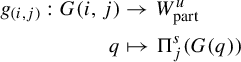 $$ \begin{align*} g_{(i,j)} : G(i,j) & \to W^u_{\textrm{part}} \\ q & \mapsto \Pi^s_j (G(q)) \end{align*} $$
for all
 $i,\,j=1,\ldots ,n$
, where
 $\Pi ^s_j$
denotes the projection along the stable leaves inside
 $R_j$
into
 $W^u_{\textrm {part}}$
. Notice that, in this case, there is no need to extend the foliations, given the existence of the Markov partition.
Verifying that this set of data defines a dynamically defined Cantor set (up to a parameterization) and that it is equal to
 $\Lambda \cap V$
for some neighborhood V of p follows from the arguments on the example above almost ‘ipsis literis’. If the boxes
 $R_j$
are sufficiently small, then one can extend the maps
 $g_{(i,j)}$
to an
 $C^{1+\varepsilon }$
expanding map g defined in a small neighborhood of the union of the pieces
 $G(i,j)$
, as the projections cannot contract distances by much. The mixing property comes from the mixing dynamics of the horseshoe. To make this conformal Cantor set to be contained in
 $W^{u}_{\varepsilon }(p)$
, all one needs to do is to apply
 $G^{-N(p)}$
a sufficient amount of times, where
 $N(p)$
is the period of p. This finishes the proof.
Remark 2.8. One can also observe that taking
 $p_f$
and
 $p_g$
as sufficiently good approximations and requiring
 $\Vert G-G_0|_{U}\Vert $
to be sufficiently small, the Cantor set obtained above, identified as
 $K_G$
, is in a small open neighborhood
 $\mathcal {V}$
of
 $K_F$
in
 $\Omega _{{P}^{\mathbb {N}}}$
. This will be important in §4.
3 A sufficient criterion for the stability of conformal Cantor sets
In this section, we explore the consequences of the conformality on the structure of the Cantor sets. The first result is the existence of limit geometries and some consequences of them. In §3.2, we define renormalization operators and verify that the limit geometries are attractors with respect to their actions. In §3.3, we use this last fact to show that the concept of recurrent compact gives a sufficient criterion for the stability of intersections between Cantor sets. All of these concepts and techniques are natural extensions from the real case.
3.1 Limit geometries
Given a conformal Cantor set K, we define
 $K(a)=K \cap G(a)$
and fix a base point
 $c(a)\in K(a)$
for all
 $a \in \mathbb {A}$
. Additionally, given
 $\underline {\theta } = ( \ldots , \theta _{-n}, \ldots , \theta _0 ) \in \Sigma ^- $
, we write
 $\underline {\theta }_n = (\theta _{-n}, \ldots , \theta _0 )$
and
 $r_{{\underline {\theta }}_n}:= \text {diam}(G^*(\underline {{\theta _n}}))$
.
As previously mentioned, we can extend g and its inverses to a neighborhood of
 $\bigsqcup _{a\in \mathbb {A}}G(a)$
, so we may consider, in the case that
 $(a_i,a_{i+1}) \in B $
,
 $f_{(a_i,a_{i+1})}$
defined from
 $ G^*(a_{i+1})$
to
 $G^*(a_i) $
; and hence also consider
 $f_{\underline {a}}: G^*(a_0) \to G^*(\underline {a})$
when
 $\underline {a}\in \Sigma ^{fin}$
. With this in mind, we can define, for any
 $\underline {\theta } \in \Sigma ^-$
and
 $n \geq 1$
:
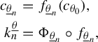 $$ \begin{align*} c_{\underline{\theta}_n} & =f_{\underline{\theta}_n}(c_{\theta_0}),\\ k^{\underline{\theta}}_n & = \Phi_{\underline{\theta}_n} \circ f_{{\underline{\theta}_n}}, \end{align*} $$
where
 $k^{\underline {\theta }}_n: G^*(\theta _0) \to \mathbb {C} $
and
 $\Phi _{\underline {\theta }_n}$
is the affine transformation over
 $\mathbb {C}$
,
 $\Phi _{\underline {\theta }_n}(z)=\alpha \cdot z + \beta , \alpha \in \mathbb {C}^*, \beta \in \mathbb {C}$
, such that
 $\Phi _{\underline {\theta }_n}( c_{\underline {\theta }_n})=0$
and
 $ D(\Phi _{\underline {\theta }_n} \circ f_{{\underline {\theta }_n}})(c_{\theta _0})=1\in \mathbb {C} $
. A transformation with these properties exists because the map g and thus its inverse branches are conformal on the set K, so
 $Df_{{\underline {\theta }_n}}(c_{\theta _0})$
is a conformal matrix that can be seen as a linear operator over
 $\mathbb {C}$
, or precisely, a multiplication by a complex number. We denote the space of affine transformations over
 $\mathbb {C}$
by
 $\textrm{Aff}(\mathbb {C})$
and consider it equipped with the
 $C^1$
topology.
Define
 $\Sigma ^-_a = \{\underline {\theta } \in \Sigma ^-, \,\underline {\theta }_0 = a \}$
and consider in this set the topology given by the metric
 $d(\underline {\theta } ^1,\underline {\theta }^2) = \text {diam}(G^*(\underline {\theta }^1 \wedge \underline {\theta }^2)) $
. Likewise, let the space
 $\text {Emb}_{1+\varepsilon }(G^*(a), \mathbb {C})$
of
 $C^{1+\varepsilon }$
embeddings from
 $G^*(a)$
to
 $\mathbb {C}$
with
 $C^{1+\varepsilon }$
inverse be equipped with the
 $C^{1+\varepsilon }$
metric.
We are also interested in the case the map g is
 $C^r$
, with
 $r \ge 2$
, so in what follows, we consider r to be a real number larger than
 $1$
. With these notation and considerations, we have the following lemma.
Lemma 3.1 (Limit geometries)
For each
 $\underline {\theta } \in \Sigma ^-$
, the sequence of
 $C^r$
embeddings
 $k^{\underline {\theta }}_n: G^*(\theta _0) \to \mathbb {C} $
converges in the
 $C^{r}$
topology to an embedding
 $ k^{\underline {\theta }}: G^*(\theta _0) \to \mathbb {C} $
. Moreover, the convergence is uniform over all
 $\underline {\theta } \in \Sigma ^-$
and in a small neighborhood of g in
 $\Omega ^r_{\Sigma }$
(see paragraph after Definition 2.2). The map
 $k: \Sigma ^-_a \to \text {Emb}(G^*(a), \mathbb {C}), \; \underline {\theta } \mapsto k^{\underline {\theta }}$
is Hölder, if we consider the metrics described above for both spaces. The
 $ k^{\underline {\theta }}: G^*(\theta _0) \to \mathbb {C} $
defined for any
 $\underline {\theta } \in \Sigma ^-$
are called the limit geometries of K.
Proof. We will first prove the result for
 $1 \leq r < 2$
. Consider for each
 $n \geq 2$
(and
 $\underline {\theta } \in \Sigma ^-$
), the functions
 $\Psi ^{\underline {\theta }}_n: {\textrm {Im}}(k^{\underline {\theta }}_{n-1}) \to \mathbb {C}$
:
 $$ \begin{align*} \Psi^{\underline{\theta}}_n= \Phi_{\underline{\theta}_n} \circ f_ {(\theta_{-n}, \theta{-n+1})}\circ \Phi_{\underline{\theta}_{n-1}}^{-1}. \end{align*} $$
Notice that
 $$ \begin{align} k^{\underline{\theta}}_n=\Psi^{\underline{\theta}}_n \circ \Psi^{\underline{\theta}}_{n-1} \circ \cdots \circ \Psi^{\underline{\theta}}_2 \circ k^{\underline{\theta}}_1. \end{align} $$
We proceed by controlling the functions
 $\Psi ^{\underline {\theta }}_n$
and showing that they are exponentially close to the identity.
First, the domain of
 $f_{(\theta _{-n}, \theta _{-n+1})}$
in the definition of
 $\Psi ^{\underline {\theta }}_n$
is
 $G^*(\underline {\theta }_{n-1})$
. Denoting its diameter by
 $r_{\underline {\theta }_{n}}$
, we know that
 $r_{\underline {\theta }_{n}} \leq C \cdot \mu ^{-n}$
for some constant
 $C>0$
, as shown in Lemma 2.1. However, we can do better. In what follows, all the C terms (with subscript, superscript, or without them) will always denote a positive real constant that will, in some way, depend on the other constants previously appearing in this proof, but never on
 $n \in \mathbb {N}$
or
 $\underline {\theta }$
. If a map f is
 $C^{1+\varepsilon }$
on an open set
 $U \subset \mathbb {C}$
, then, for any point
 $z \in U$
and
 $h \in \mathbb {C}$
small enough so that the segment joining z and
 $z+h$
is in U:
 $$ \begin{align*} |f(z+h)-(f(z)+Df(z)\cdot h)| < \tilde{C} |h|^{1+\varepsilon}, \end{align*} $$
for some constant
 $\tilde {C}> 0$
. Consequently,
 $ f_{(\theta _{-n}, \theta _{-n+1})}:G^*(\underline {\theta }_{n-1}) \to G^*(\underline {\theta }_n)$
is
 $C_f \cdot r_{\underline {\theta }_{n-1}}^{1+\varepsilon }$
close to the map
 $A_{\underline {\theta }_n} \in \textrm{Aff}(\mathbb {C})$
described by
 $$ \begin{align*}A_{\underline{\theta}_n}(c_{\underline{\theta}_{n-1}})=c_{\underline{\theta}_n} \quad\text{and}\quad DA_{\underline{\theta}_n} = Df_{(\theta_{-n}, \theta_{-n+1})}(c_{\underline{\theta}_{n-1}}),\end{align*} $$
and thus, if n is large enough:
 $$ \begin{align*} r_{\underline{\theta}_{n}} & \leq |Df_{(\theta_{-n}, \theta_{-n+1})}(c_{\underline{\theta}_{n-1}})|\cdot\, r_{\underline{\theta}_{n-1}} + C_f \cdot r_{\underline{\theta}_{n-1}}^{1+\varepsilon} \\ & \leq r_{\underline{\theta}_{n-1}} \cdot ( | Df_{(\theta_{-n}, \theta_{-n+1})}(c_{\underline{\theta}_{n-1}}) | + C_1 \cdot \mu^{(-n+1)\varepsilon}). \end{align*} $$
Arguing by induction, using that
 $\log {(x+y)} \le \log {x} +({y}/{x})$
, we obtain
 $$ \begin{align*} &\log r_{\underline{\theta}_{n}} \leq \log |Df_{\underline{\theta}_n}(c_{\theta_0})| + \Vert Dg\Vert \cdot \sum_{j=0}^{n-1} ( C_1 \cdot \mu^{-j\varepsilon} ) \leq \log |Df_{\underline{\theta}_n}(c_{\theta_0})| + C_2 , \end{align*} $$
so
 $$ \begin{align*} r_{\underline{\theta}_{n}} \leq C' \cdot | Df_{\underline{\theta}_n}(c_{\theta_0})| \leq C' \cdot \mu^{-n}, \end{align*} $$
because
 $|Df_{(\theta _{-n}, \theta _{-n+1})}(x)|^{-1} \le \lVert Dg \rVert \; \text { for all } x \in G^*(\theta _{-n+1})$
, where
 $\lVert Dg \rVert $
denotes the
 $C^0$
norm of this function over its domain. In a completely analogous way, we can show, maybe enlarging
 $C'$
, that
 $$ \begin{align} {C'}^{-1} \cdot |Df_{\underline{\theta}_n}(c_{\theta_0})| \leq r_{\underline{\theta}_{n}} \leq C' \cdot |Df_{\underline{\theta}_n}(c_{\theta_0})| \end{align} $$
and so the size of the
 $G^*(\underline {\theta }_n)$
is controlled. This implies that
 $$ \begin{align*} \Vert f_{(\theta_{-n}, \theta_{-n+1})}-A_{\underline{\theta}_n}\Vert \leq C \cdot |Df_{\underline{\theta}_n}(c_{\theta_0})|^{1+\varepsilon} \end{align*} $$
for some constant C, for all
 $\underline {\theta } \in \Sigma ^-$
. However, by construction,
 $ \Phi _{\underline {\theta }_n} \circ A_{\underline {\theta }_n} \circ \Phi _{\underline {\theta }_{n-1}}^{-1} = {\textrm {Id}}$
and
 $ D\Phi _{\underline {\theta }_n} = (Df_{{\underline {\theta }_n}}(c_{\theta _0}))^{-1} $
; therefore,
 $$ \begin{align*} \Vert \Psi^{\underline{\theta}}_n -{\textrm{Id}}\Vert & = \Vert \Psi^{\underline{\theta}}_n -\Phi_{\underline{\theta}_n}\circ A_{\underline{\theta}_n} \circ \Phi_{\underline{\theta}_{n-1}}^{-1} \Vert \leq \Vert D\Phi_{\underline{\theta}_n}\Vert \cdot \Vert f_{(\theta_{-n}, \theta_{-n+1})}-A_{\underline{\theta}_n} \Vert \\ & \leq |Df_{{\underline{\theta}_n}}(c_{\theta_0})|^{-1} \cdot C \cdot |Df_{\underline{\theta}_{n-1}}(c_{\theta_0})|^{1+\varepsilon}\\ & \leq C_3 \cdot {(\mu^{-\varepsilon})}^n \end{align*} $$
as we wished to obtain. This is enough to show that
 $\{k^{\underline {\theta }}_n\}_{n\geq 0}$
is a Cauchy sequence, at least in
 $C^0$
metric. In fact, for
 $m,l \geq 1$
,
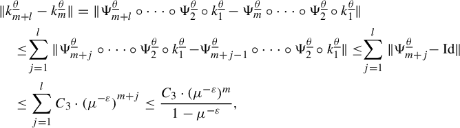 $$ \begin{align*} &\Vert k^{\underline{\theta}}_{m+l}-k^{\underline{\theta}}_m\Vert = \Vert \Psi^{\underline{\theta}}_{m+l} \circ \cdots \circ \Psi^{\underline{\theta}}_2 \circ k^{\underline{\theta}}_1 - \Psi^{\underline{\theta}}_{m} \circ \cdots \circ \Psi^{\underline{\theta}}_2 \circ k^{\underline{\theta}}_1 \Vert \\ & \quad\leq\! \sum_{j=1}^l \Vert \Psi^{\underline{\theta}}_{m+j} \circ \cdots \circ \Psi^{\underline{\theta}}_2 \circ k^{\underline{\theta}}_1 -\! \Psi^{\underline{\theta}}_{m+j-1} \circ \cdots \circ \Psi^{\underline{\theta}}_2 \circ k^{\underline{\theta}}_1 \Vert \leq\! \sum_{j=1}^l \Vert \Psi^{\underline{\theta}}_{m+j} \!-{\textrm{Id}} \Vert \\ &\quad \leq \sum_{j=1}^l C_3 \cdot {(\mu^{-\varepsilon})}^{m+j} \leq \frac{C_3 \cdot (\mu^{-\varepsilon})^{m}}{1-\mu^{-\varepsilon}}, \end{align*} $$
which implies that
 $\Vert k^{\underline {\theta }}_{m+l}-k^{\underline {\theta }}_m\Vert \rightarrow 0$
as
 $m \rightarrow \infty $
. Further, for any point
 $z \in {\textrm {Im}}(k^{\underline {\theta }}_{n-1})$
, we can calculate
 $ D\Psi ^{\underline {\theta }}_n (z) = D\Phi _{\underline {\theta }_n} \cdot Df_{(\theta _{-n, \theta {-n+1}})} ( \Phi _{\underline {\theta }_{n-1}}^{-1} (z) ) \cdot D\Phi _{\underline {\theta }_{n-1}}^{-1}$
. However, by hypothesis, we have that
 $D\Psi ^{\underline {\theta }}_n (c_{\theta _0}) = {\textrm {Id}}$
and
 $$ \begin{align*}d(\Phi_{\underline{\theta}_{n-1}}^{-1} (z),\Phi_{\underline{\theta}_{n-1}}^{-1} (c_{\theta_0})) \leq \text{diam} (G^* (\underline{\theta}_{n-1})). \end{align*} $$
Then, using that
 $Df_{(\theta _{-n, \theta {-n+1}})}$
is
 $\varepsilon $
-Hölder, we conclude that
 $$ \begin{align} \Vert D\Psi^{\underline{\theta}}_n -{\textrm{Id}}\Vert \leq C_f \cdot |D\Phi_{\underline{\theta}_n}| \cdot |D\Phi_{\underline{\theta}_{n-1}}|^{-1} \cdot r_{\underline{\theta}_{n-1}}^{\varepsilon} \leq C_4 \mu^{-n \varepsilon} , \end{align} $$
because
 $|D\Phi _{\underline {\theta }_n}|$
and
 $|D\Phi _{\underline {\theta }_{n-1}}|$
are comparable (because
 $D\Phi _{\underline {\theta }_n}= Df_{\underline {\theta }_{n}}(c_{\theta _0})^{-1}$
and so
 $|D\Phi _{\underline {\theta }_n}| \cdot |D\Phi _{\underline {\theta }_{n-1}}|^{-1}$
is controlled by
 $\Vert Dg\Vert $
).
Now we can show that
 $\{\Vert Dk^{\underline {\theta }}_n\Vert \}_{n \geq 1}$
is bounded. Indeed,
 $\Vert Dk^{\underline {\theta }}_n \Vert \leq \prod _{j\geq 2} ^ {n}\Vert D\Psi ^{\underline {\theta }}_j \Vert \cdot \Vert Dk^{\underline {\theta }}_1 \Vert $
implies that:
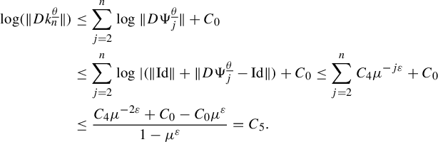 $$ \begin{align*} \log ( \Vert Dk^{\underline{\theta}}_n \Vert ) & \leq {\sum_{j=2}^{n} \log \Vert D\Psi^{\underline{\theta}}_j \Vert } + C_0 \\ & \leq {\sum_{j=2}^{n} \log |(\Vert {\textrm{Id}}\Vert +\Vert D\Psi^{\underline{\theta}}_j - {\textrm{Id}}\Vert ) } + C_0 \leq {\sum_{j=2}^{n} C_4 \mu^{-j \varepsilon} } + C_0 \\ & \leq \frac{C_4\mu^{-2\varepsilon}+C_0-C_0\mu^{\varepsilon}}{1-\mu^{\varepsilon}} = C_5. \end{align*} $$
The same argument can be used to show that
 $\Vert (Dk^{\underline {\theta }}_n)^{-1}\Vert $
is bounded. It also follows that:
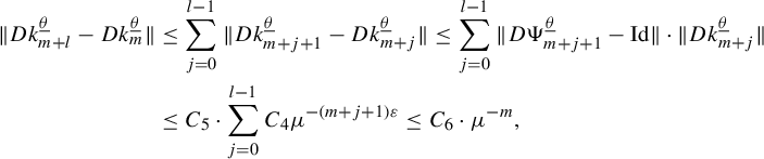 $$ \begin{align*} \Vert Dk^{\underline{\theta}}_{m+l}-Dk^{\underline{\theta}}_{m}\Vert & \leq \sum_{j=0}^{l-1} \Vert Dk^{\underline{\theta}}_{m+j+1}-Dk^{\underline{\theta}}_{m+j}\Vert \leq \sum_{j=0}^{l-1} \Vert D\Psi^{\underline{\theta}}_{m+j+1}-{\textrm{Id}}\Vert \cdot \Vert Dk^{\underline{\theta}}_{m+j}\Vert \\ & \leq C_5 \cdot {\sum_{j=0}^{l-1} C_4 \mu^{-(m+j+1) \varepsilon} } \leq C_6 \cdot \mu^{-m}, \end{align*} $$
which shows that
 $\{k^{\underline {\theta }}_n\}_{n\geq 0}$
is a Cauchy sequence also in the
 $C^1$
metric, and so it converges to a
 $C^1$
map
 $ k^{\underline {\theta }}$
. Because
 $\Vert (Dk^{\underline {\theta }}_n)^{-1}\Vert $
is bounded, this also implies that the inverse maps
 $\{(k^{\underline {\theta }}_n)^{-1}_{n\geq 0}\}$
also converge in the
 $C^1$
metric to the inverse of
 $k^{\underline {\theta }}$
.
We need to show that
 $ k^{\underline {\theta }}$
is
 $C^{1+\varepsilon }$
. This is true for
 $k^{\underline {\theta }}_{n}$
for all
 $n \geq 0$
. Indeed, for a given
 $\underline {\theta } \in \Sigma ^-$
, we write for
 $n \geq 0,\, x, y \in G^*(\theta _0)$
’:
 $$ \begin{align*}I_{n}(x,y)=|Dk^{\underline{\theta}}_{n}(x)-Dk^{\underline{\theta}}_{n}(y)| < H_n \cdot |x-y|^{\varepsilon}, \end{align*} $$
for some constant
 $H_n>0$
. By equations (3.1), (3.3), and the fact that
 $Dk^{\underline {\theta }}_{n}$
are bounded, we have that:
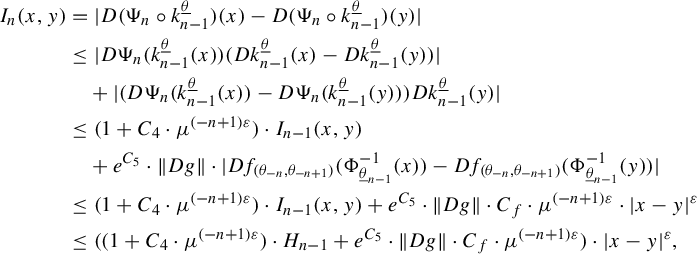 $$ \begin{align*} I_{n} (x,y) & = | D(\Psi_n \circ k^{\underline{\theta}}_{n-1})(x)-D(\Psi_n \circ k^{\underline{\theta}}_{n-1})(y) |\\ & \leq | D\Psi_n (k^{\underline{\theta}}_{n-1}(x)) (Dk^{\underline{\theta}}_{n-1}(x)-Dk^{\underline{\theta}}_{n-1}(y) ) | \\ & \quad + | ( D\Psi_n(k^{\underline{\theta}}_{n-1}(x))- D\Psi_n (k^{\underline{\theta}}_{n-1} (y)))Dk^{\underline{\theta}}_{n-1}(y) |\\ & \leq (1+C_4\cdot\mu^{(-n+1)\varepsilon})\cdot I_{n-1}(x,y) \\ & \quad+ e^{ C_5} \cdot \Vert Dg\Vert \cdot | Df_{(\theta_{-n}, \theta_{-n+1})}(\Phi_{\underline{\theta}_{n-1}}^{-1}(x)) - Df_{(\theta_{-n}, \theta_{-n+1})}(\Phi_{\underline{\theta}_{n-1}}^{-1}(y))|\\ & \leq (1+C_4\cdot\mu^{(-n+1)\varepsilon})\cdot I_{n-1}(x,y) + e^{C_5}\cdot \Vert Dg\Vert \cdot C_f \cdot \mu^{(-n+1)\varepsilon} \cdot |x-y|^{\varepsilon}\\ & \leq ((1+C_4\cdot\mu^{(-n+1)\varepsilon})\cdot H_{n-1}+ e^{C_5} \cdot \Vert Dg\Vert \cdot C_f \cdot \mu^{(-n+1)\varepsilon} )\cdot |x-y|^{\varepsilon}, \end{align*} $$
which inductively shows that these functions have Hölder continuous derivatives. Additionally, we can choose the Hölder constants satisfying the relation:
 $$ \begin{align} H_n \leq (1+C_4\cdot\mu^{(-n+1)\varepsilon}) \cdot H_{n-1}+ C_7 \cdot \mu^{(-n+1)\varepsilon}, \end{align} $$
and then the sequence
 $\{ H_n \}_{n \geq 1}$
is bounded. Effectively, it is crescent and if
 $H_{n-1}> 1 $
, then
 $H_n \leq (1+C_4\cdot \mu ^{(-n+1)\varepsilon } + C_7 \cdot \mu ^{(-n+1)\varepsilon }) \cdot H_{n-1} \leq (1+C_8\cdot \mu ^{(-n+1)\varepsilon }) \cdot H_{n-1}$
and using the same strategy as above, we have
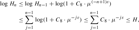 $$ \begin{align*} \log H_n & \leq \log H_{n-1} + \log (1+C_8\cdot\mu^{(-n+1)\varepsilon}) \\ & \leq \sum_{j=1}^{n-1} \log (1+C_8\cdot\mu^{-j\varepsilon}) \leq \sum_{j=1}^{n-1} C_8\cdot\mu^{-j\varepsilon} \leq H, \end{align*} $$
as stated.
Finally, for each pair
 $x,y \in G^*(\theta _0)$
, there is
 $n\geq 0$
such that
 $\Vert Dk^{\underline {\theta }}_{n}-Dk^{\underline {\theta }}\Vert $
is less than
 $|x-y|^{\varepsilon }$
so, by triangle inequality, we have
 $|Dk^{\underline {\theta }}(x)-Dk^{\underline {\theta }}(y)| < (H+2) \cdot |x-y|^{\varepsilon }$
. By maybe enlarging H a little, the same estimates are true for the inverses of
 $k^{\underline {\theta }_n}$
and
 $k^{\underline {\theta }}$
.
Now, because the maps
 $k^{\underline {\theta }}$
are
 $C^{1+\varepsilon }$
, to prove that the sequence
 $k^{\underline {\theta }}_n$
converges to
 $k^{\underline {\theta }}$
in the
 $C^{1+\varepsilon }$
topology, it is sufficient to show that
 $$ \begin{align} \lim_{n \rightarrow \infty} \mathop{\mathrm{sup}}\limits_{x, y \in k^{\underline{\theta}}(G^*(\theta_0))} \frac{ \lvert {D( k^{\underline{\theta}}_n \circ (k^{\underline{\theta}})^{-1})(x)} - {D ( k^{\underline{\theta}}_n \circ (k^{\underline{\theta}})^{-1})}(y) \rvert } {\lvert x - y \rvert^\varepsilon } = 0. \end{align} $$
For a fixed value of
 $n> 0 $
, let
 $\underline {\theta }^n \in \Sigma ^-$
be the infinite word such that
 $\underline {\theta } = \underline {\theta }^n\underline {\theta }_n$
. Consequently, for
 $m> n$
,
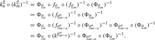 $$ \begin{align*} k^{\underline{\theta}}_n\circ (k^{\underline{\theta}}_m)^{-1} & = \Phi_{\underline{\theta}_n} \circ f_{\underline{\theta}_n} \circ (f_{\underline{\theta}_{m}})^{-1} \circ (\Phi_{\underline{\theta}_m})^{-1} \\ & = \Phi_{\underline{\theta}_n} \circ (f_{\underline{\theta}^n_{m - n}})^{-1} \circ (\Phi_{\underline{\theta}_m})^{-1} \\ & = \Phi_{\underline{\theta}_n} \circ (f_{\underline{\theta}^n_{m - n}})^{-1} \circ (\Phi_{\underline{\theta}^{n}_{m-n}})^{-1} \circ \Phi_{\underline{\theta}^{n}_{m-n}} \circ (\Phi_{\underline{\theta}_m})^{-1} \\ & = \Phi_{\underline{\theta}_n} \circ (k^{\underline{\theta}^n_{m - n}})^{-1} \circ \Phi_{\underline{\theta}^{n}_{m-n}} \circ (\Phi_{\underline{\theta}_m})^{-1}. \end{align*} $$
Remember that
 $ (D\Phi _{\underline {\theta }^n_{m-n}})^{-1} = Df_{\underline {\theta }^n_{m - n}}(c_{\theta _{-n}})$
has norm comparable to
 $r_{\underline {\theta }^n_{m-n}}$
. Now, because
 $f_{\underline {\theta }_n}(c_{\theta _0})$
could also be chosen as the base point for the piece
 $G(\theta _{-n})$
, equation (3.2) implies that
 $\lvert Df_{\underline {\theta }^n_{m - n}}(f_{\underline {\theta }_n}(c_{\theta _0})) \rvert $
is also comparable to
 $r_{\underline {\theta }^n_{m-n}}$
, and so
 $\lvert D ( \Phi _{\underline {\theta }^{n}_{m-n}} \circ (\Phi _{\underline {\theta }_m})^{-1} ) \rvert $
is comparable to
 $\lvert \Phi _{\underline {\theta }_n}^{-1} \rvert $
. Therefore, for
 $x, y \in k^{\underline {\theta }_m}(G^*(\theta _0))$
,
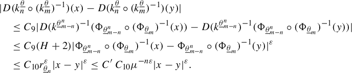 $$ \begin{align*} &\lvert D(k^{\underline{\theta}}_n\circ (k^{\underline{\theta}}_m)^{-1} )(x) - D(k^{\underline{\theta}}_n\circ (k^{\underline{\theta}}_m)^{-1})(y) \rvert \\ &\quad\le C_9 \lvert D(k^{\underline{\theta}^n_{m - n}})^{-1} (\Phi_{\underline{\theta}^{n}_{m-n}} \circ (\Phi_{\underline{\theta}_m})^{-1}(x)) - D(k^{\underline{\theta}^n_{m - n}})^{-1} (\Phi_{\underline{\theta}^{n}_{m-n}} \circ (\Phi_{\underline{\theta}_m})^{-1} ( y) )\rvert \\ &\quad\le C_{9} (H+2) \lvert \Phi_{\underline{\theta}^{n}_{m-n}} \circ (\Phi_{\underline{\theta}_m})^{-1}(x) - \Phi_{\underline{\theta}^{n}_{m-n}} \circ (\Phi_{\underline{\theta}_m})^{-1}(y) \rvert^{\varepsilon} \\ &\quad\le C_{10} r_{\underline{\theta}_n}^{\varepsilon} \lvert x - y \rvert^{\varepsilon} \le C'\,C_{10} \mu^{-n\varepsilon} \lvert x - y \rvert^\varepsilon. \end{align*} $$
Finally, making
 $m \rightarrow \infty $
and then
 $n \rightarrow \infty $
, we prove the limit (3.5).
All the constants appearing in the estimates above depend continuously (actually, they are simple functions) on the
 $C^1$
norm of g as well as the Hölder constant and exponent of
 $Dg$
, and so, for any
 $g'$
sufficiently close to g, all of those estimates would be the same except with a minor pre-fixed error. This implies that the convergence we just showed is uniform not only over
 $\Sigma ^-$
but also on a small neighborhood of g in the Hölder topology.
The Hölder continuity of the association
 $\underline {\theta } \mapsto k^{\underline {\theta }}$
comes from the fact that, for some constant
 $C_{12}> 0$
,
 $$ \begin{align} \lVert k^{\underline{\theta}} - k^{\underline{\theta}}_n \rVert_{C^{1+\varepsilon}} \le C_{12}r_{\underline{\theta}_n}^{\varepsilon}, \end{align} $$
from which, for any
 $\underline {\theta }^1, \, \underline {\theta }^2 \in \Sigma ^-$
,
 $$ \begin{align*} \lVert k^{\underline{\theta}^1} - k^{\underline{\theta}^2} \rVert_{C^{1+\varepsilon}} \le 2C_{12}r_{\underline{\theta}^1 \wedge \underline{\theta}^2}^{\varepsilon} = 2C_{12} d(\underline{\theta}^1, \underline{\theta}^2)^{\varepsilon}. \end{align*} $$
Equation (3.6) is a consequence of the fact that for
 $x, y\in k^{\underline {\theta }}(G^*(\theta _0))$
,
 $$ \begin{align*} \lvert D(k^{\underline{\theta}}_n\circ (k^{\underline{\theta}})^{-1})(x) - D(k^{\underline{\theta}}_n\circ (k^{\underline{\theta}})^{-1})(y)\rvert \le C_{10} r_{\underline{\theta}_n}^{\varepsilon} \lvert x - y \rvert^{\varepsilon} \end{align*} $$
and with just a small refinement of the estimates made above for
 $$ \begin{align*} \lVert k^{\underline{\theta}}_{m+l} - k^{\underline{\theta}}_{m}\rVert \quad \text{and} \quad \lVert Dk^{\underline{\theta}}_{m+l}-Dk^{\underline{\theta}}_{m} \rVert \end{align*} $$
for
 $m, l> 0$
. Indeed, the terms in the series
 $$ \begin{align*} \sum_{j=0}^{l-1} \lVert \Psi^{\underline{\theta}}_{m+j+1}-{\textrm{Id}} \rVert \quad \text{and} \quad \sum_{j=0}^{l-1} \lVert D\Psi^{\underline{\theta}}_{m+j+1}-{\textrm{Id}} \rVert \end{align*} $$
decay exponentially; therefore, these series can be controlled by
 $\lVert \Psi ^{\underline {\theta }}_{m}-{\textrm {Id}} \rVert $
and
 $\lVert D \Psi ^{\underline {\theta }}_{m}-{\textrm {Id}} \rVert $
, respectively.
If the map g defining the Cantor set is
 $C^r, r \geq 2$
, then the convergence also happens in the
 $C^r$
metric. This happens because the composition with affine maps on the definition of
 $\Psi ^{\underline {\theta }}_n$
‘flattens’ the derivatives of
 $f_{(\theta _{-n}, \theta _{-n+1})}$
. As we have seen above, the first-order derivatives of the maps
 $\Psi ^{\underline {\theta }}_n$
are close to the identity, or close (in norm) to
 $1=r_{\underline {\theta }_n}^0$
. Analogously, the derivatives of order
 $r \in \mathbb {N}$
have norm less than
 $r_{\underline {\theta }_n}^{r-1}$
. A formula for the derivatives of higher order of a composition of two maps can be found in [Reference Constantine and Savits5]. It allow us to inductively bound the
 $C^r$
norm of
 $ k^{\underline {\theta }}_{n}$
, if r is an integer, and the convergence
 $k^{\underline {\theta }_n} \rightarrow k^{\underline {\theta }}$
is proved in this metric following the same type of argument in this proof. Moreover, following the same strategy as above, one can also show that if
 $r \notin \mathbb {N}$
is greater than
 $2$
, the maps
 $D^{\lfloor r \rfloor }k^{\underline {\theta }}$
are
 $r-\lfloor r \rfloor $
Hölder and that the convergence also happens in the
 $C^r$
metric, which completes the proof. The key is to analyze, in the expression of
 $D^{\lfloor r \rfloor }(f \circ g)$
, the terms involving derivatives of order
 $\lfloor r \rfloor $
of f and g. In the end, we have expressions similar to those in the proof, only involving many more terms.
As an immediate consequence of equation (3.2) in the previous proof, we have the following bounded distortion property.
Corollary 3.2 There is a constant
 $C>0$
such that for every pair of points
 $c_1,\, c_2 \in K(a)$
,
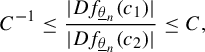 $$ \begin{align*} C^{-1 }\leq \frac{|Df_{\underline{\theta}_n}(c_1)|}{|Df_{\underline{\theta}_n}(c_2)|} \leq C, \end{align*} $$
for all
 $\underline {\theta }_n =(\theta _{-n},\ldots , \theta _0)\in \Sigma ^{fin}$
with
 $\theta _0=a$
.
Notice that the limit geometries depend on the choice of the base point
 $c_{\theta _0}$
, because the maps
 $\Psi ^{\underline {\theta }}_n$
depend on it. However, Corollary 3.2 shows that for different choices of base point, the norm of the expansion factor of
 $\Phi _{\underline {\theta }_n}$
is bounded between
 $|C^{-1} \cdot Df_{\underline {\theta }_n}(c_{\theta _0})|$
and
 $|C \cdot Df_{\underline {\theta }_n}(c_{\theta _0})|$
for a fixed choice of
 $c_{\theta _0}$
. Because these maps also send the base point to
 $0$
, we have that different choices of base points
 $c_1$
and
 $c_2$
result in different limit geometries that are related by
 $$ \begin{align*} k^{\underline{\theta}}_1 = A \cdot k^{\underline{\theta}}_2 , \end{align*} $$
where A is a map in
 $\textrm{Aff}(\mathbb {C})$
whose coefficients are bounded by some constant
 $C> 0$
. So, up to (bounded) affine transformations, the limit geometries do not depend on the base point. Every time we mention the limit geometries of a Cantor set, consider that a set of base points has already been fixed. Also, we could choose to define
 $\Phi _{\underline {\theta }_n}$
as the affine map such that
 $\Phi _{\underline {\theta }_n}( c_{\underline {\theta }_n})=0$
,
 $ |D\Phi _{\underline {\theta }_n}|^{-1} =\text {diam}( G^*(\underline {\theta }_n)) $
, and
 $D\Phi _{\underline {\theta }_n}(c_{\theta _0})(1,0) \in \mathbb {R}^*_{+} \subset \mathbb {R}^2$
, and the resulting limit geometries would only differ from those defined as above by bounded affine transformations. This may be the definition on some other sources.
The bounded distortion property can be improved as follows.
Corollary 3.3 There is a constant
 $C> 0$
such that for every pair of points
 $x,\,y \in G^*(\theta _0)$
,
 $$ \begin{align*} \frac{|Df_{\underline{a}}(x)|}{m(Df_{\underline{a}}(y))} \leq C \quad\text{and}\quad C^{-1} \leq \frac{m(Df_{\underline{a}}(x))} {|Df_{\underline{a}}(y)|}, \end{align*} $$
for all
 $ \underline {a}=(a_0,a_1, \ldots , a_n) \in \Sigma ^{fin}$
. A larger value of n and the closer
 $x, y$
are to each other will result in the closer the ratios of
 ${|Df_{\underline {a}}(x)|}/{|Df_{\underline {a}}(y)|}$
and
 ${m(Df_{\underline {a}}(x))}/{m(Df_{\underline {a}}(y))} $
are to
 $1$
.
Proof. Given any
 $\underline {\theta }$
whose ending coincides with the word
 $\underline {a}$
, by the estimates in the proof of Lemma 3.1, there is some constant
 $C_{13}> 0$
such that
 $$ \begin{align*} \log{\lvert D (k^{\underline{\theta}}_n \circ (k^{\underline{\theta}})^{-1})(z)\rvert} \,\, \leq C_{13} \cdot r_{{\underline{\theta}}_n}^{\varepsilon} \quad \text{and} \quad \log{\lvert D (k^{\underline{\theta}} \circ (k^{\underline{\theta}}_n)^{-1})(z')\rvert} \,\, \leq C_{13} \cdot r_{{\underline{\theta}}_n}^{\varepsilon} \end{align*} $$
for
 $z \in k^{\underline {\theta }}(G^{*}(\theta _0)) $
and
 $z' \in k^{\underline {\theta }}_n(G^{*}(\theta _0)) $
. Making
 $z=k^{\underline {\theta }}(x)$
and
 $z'=k^{\underline {\theta }}_n(y)$
, it follows that
 $$ \begin{align} \log{\lvert Dk^{\underline{\theta}}_n(x)\cdot(Dk^{\underline{\theta}}(x))^{-1}\rvert + \log{\lvert Dk^{\underline{\theta}}(y)\cdot(Dk^{\underline{\theta}}_n(y))^{-1} \rvert}} \le 2C_9 \cdot r_{{\underline{\theta}}_n}^{\varepsilon}, \end{align} $$
and so, using that
 $ \lvert A \rvert \cdot m(B) \le \lvert A \cdot B \rvert $
and
 $m(A) \cdot \lvert B \rvert \le \lvert A \cdot B \rvert $
for any two square matrices,
 $$ \begin{align*} \log{\lvert Dk^{\underline{\theta}}_n(x)\rvert} + \log{m((Dk^{\underline{\theta}}(x))^{-1})} + \log{m(Dk^{\underline{\theta}}(y))} +\log{\lvert (Dk^{\underline{\theta}}_n(y))^{-1}\rvert} \le 2C_9 \cdot r_{{\underline{\theta}}_n}^{\varepsilon}.\end{align*} $$
However, by the definition of
 $k^{\underline {\theta }}_n$
and the fact that
 $m(A^{-1})=\lvert A \rvert ^{-1}$
for any invertible matrix A,
 $$ \begin{align} \frac{|Df_{\underline{a}}(x)|}{m(Df_{\underline{a}}(y))}=\lvert Dk^{\underline{\theta}}_n(x)\rvert \cdot \lvert (Dk^{\underline{\theta}}_n(y))^{-1} \rvert \le \frac{\lvert Dk^{\underline{\theta}}(x) \rvert}{m(Dk^{\underline{\theta}}(y))} \exp{(2C_9 \cdot r_{{\underline{\theta}}_n}^{\varepsilon})}, \end{align} $$
for any
 $x,\, y \in G^*(\theta _0)$
. As the association
 $\underline {\theta } \mapsto k^{\underline {\theta }}$
is continuous and
 $\Sigma ^-$
is compact, there is
 $C>0$
that bounds the right-hand side of equation (3.8) for all
 $x,\,y \in G^{*}(\theta _0)$
and
 $n \in \mathbb {N}$
. The second part is obtained in an analogous way, only changing the way we proceed from equation (3.7). In the case of the operator norm, it yields
 $$ \begin{align*} \log{\lvert Dk^{\underline{\theta}}_n(x)\rvert} + \log{m((Dk^{\underline{\theta}}(x))^{-1})} + \log{\lvert Dk^{\underline{\theta}}(y)\rvert} +\log{m( (Dk^{\underline{\theta}}_n(y))^{-1})} \le 2C_9 \cdot r_{{\underline{\theta}}_n}^{\varepsilon}, \end{align*} $$
from which
 $$ \begin{align*} \frac{|Df_{\underline{a}}(x)|}{|Df_{\underline{a}}(y)|} \le \frac{\lvert Dk^{\underline{\theta}}(x) \rvert}{\lvert Dk^{\underline{\theta}}(y) \rvert } \exp{(2C_9 \cdot r_{{\underline{\theta}}_n}^{\varepsilon})}, \end{align*} $$
and the claim follows because of the continuity of
 $k^{\underline {\theta }}(x)$
on
 $\underline {\theta }$
and x.
We also have the following result.
Corollary 3.4 The diameter of the sets
 $G^*(\underline {\theta }_n)$
is of order
 $\Vert Df_{\underline {\theta }_n}\Vert $
.
We end this section with the following lemma, which shows continuous dependence of limit geometries on the map g defining the Cantor set.
Lemma 3.5 For any Cantor set K given by a map
 $g \in \Omega _{\Sigma }$
and any
 $\varepsilon> 0$
, there is a small
 $\delta> 0$
satisfying the following: for any map
 $\tilde {g} \in U_{K, \delta }$
, there is a choice of base points
 $\tilde {c}_a \in \tilde {G}(a)$
for all
 $a \in \mathbb {A}$
, each of them close to the already fixed points
 $c_a \in G(a)$
, in a manner that the resultant limit geometries associated to these choices satisfy
 $\Vert \tilde {k}^{\underline {\theta }}-{k}^{\underline {\theta }}\Vert _{C^1} < \varepsilon $
in the largest domain both maps are defined for all
 $\underline {\theta }\in \Sigma ^-$
.
Proof. First, we can consider
 $c_a \in \textrm{int} \, G(a)$
. This can be done because of the additional hypothesis on the sets
 $G(a)$
, described at the end of §2.1, just before Definition 2.2. By the definition of
 $U_{K,\delta '}$
, we can choose
 $\tilde {c}_a$
such that
 $H(c_a)= \tilde {H}(\tilde {c}_a)$
, where
 $H: K \to \Sigma $
is the homeomorphism defined just after Definition 2.1, which implies
 $|\tilde {c}_a-c_a|< \delta $
for every
 $\delta '$
sufficiently small. Let us analyze the limit of
 $\Vert \tilde {k}_n^{\underline {\theta }}-{k}_n^{\underline {\theta }}\Vert _{C^0}$
.
Define
 $x_n = \Vert \tilde {k}_{n}^{\underline {\theta }}-{k}_{n}^{\underline {\theta }}\Vert _{C^0}$
for
 $n \in \mathbb {N}$
. Given
 $\varepsilon _0>0$
and
 $N \in \mathbb {N}$
, if the distance between
 $k_1^{\underline {\theta }}$
and
 $\tilde {k}_1^{\underline {\theta }}$
is small enough and so is
 $\delta '$
, then, by continuity,
 $x_n = \Vert \tilde {k}_n^{\underline {\theta }}-{k}_n^{\underline {\theta }}\Vert _{C^0} < \varepsilon _0$
for all
 $n \leq N$
. We will prove by induction that if
 $n\geq N$
, then there are constants
 $\tilde {C}_1$
,
 $\tilde {C}_2$
and
 $0<\lambda <1$
such that
 $$ \begin{align} x_{n+1}\leq (1+\tilde{C}_1\lambda^n)x_n + \tilde{C}_2 \lambda^n, \end{align} $$
and, for all
 $n \geq N$
, we can apply
 $\Psi _{n+1}^{\underline {\theta }}$
to the image of
 $\tilde {k}_n^{\underline {\theta }}$
. It is not true that we can always apply
 $\Psi _{N+1}^{\underline {\theta }}$
to the image of
 $\tilde {k}_N^{\underline {\theta }}$
; at least not considering the same domain
 ${\textrm {Im}}(k^{\underline {\theta }_N})$
used in the definition at the beginning of the proof of Lemma 3.1. However, this domain can be extended to a larger set
 $V_{\varepsilon _1}({\textrm {Im}}(k^{\underline {\theta }_N}))$
, for some
 $\varepsilon _1>0$
, simply because
 $$ \begin{align*} \Psi^{\underline{\theta}}_n= \Phi_{\underline{\theta}_n} \circ f_ {(\theta_{-n}, \theta{-n+1})}\circ \Phi_{\underline{\theta}_{n-1}}^{-1} \end{align*} $$
is well defined on
 $\Phi _{\underline {\theta }_{n-1}} (G(\theta _{-n+1})) \supset \Phi _{\underline {\theta }_{n-1}} (G(\underline {\theta }_{-n+1})) = {\textrm {Im}}(k^{\underline {\theta _n}})$
. So by making
 $N=n$
and observing that we can make
 $x_N \leq \varepsilon _0$
, the first part of the basis of induction is proved. Now, if we can apply
 $\Psi _{n+1}^{\underline {\theta }}$
to the image of
 $\tilde {k}_n^{\underline {\theta }}$
for some
 $n \geq N$
, we have, following the notation in the proof of Lemma 3.1, that
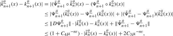 $$ \begin{align} |\tilde{k}_{n+1}^{\underline{\theta}}(x)-{k}_{n+1}^{\underline{\theta}}(x)| & = |(\tilde{\Psi}_{n+1}^{\underline{\theta}}\circ\tilde{k}_{n}^{\underline{\theta}})(x)-({\Psi}_{n+1}^{\underline{\theta}}\circ{k}_{n}^{\underline{\theta}})(x)|\nonumber\\ & \leq |\Psi_{n+1}^{\underline{\theta}}(\tilde{k}_{n}^{\underline{\theta}}(x))-{\Psi}_{n+1}^{\underline{\theta}}({k}_{n}^{\underline{\theta}}(x))| + |(\tilde{\Psi}_{n+1}^{\underline{\theta}}- {\Psi}_{n+1}^{\underline{\theta}})(\tilde{k}_{n}^{\underline{\theta}}(x))| \nonumber\\ & \leq \Vert D{\Psi}_{n+1}^{\underline{\theta}}\Vert \cdot|\tilde{k}_{n}^{\underline{\theta}}(x)-{k}_{n}^{\underline{\theta}}(x)| + \Vert \tilde{\Psi}_{n+1}^{\underline{\theta}}- {\Psi}_{n+1}^{\underline{\theta}} \Vert \nonumber\\ & \leq (1+C_4 \mu^{-n \varepsilon}) \cdot|\tilde{k}_{n}^{\underline{\theta}}(x)-{k}_{n}^{\underline{\theta}}(x)| + 2 C_3 \mu^{-n \varepsilon}, \end{align} $$
which yields an estimate of the type in equation (3.9), and so, the induction basis is complete. However, with basic real analysis, one can show that there are constants
 $\tilde {C}_3$
and
 $\tilde {C}_4$
independent of
 $m \in \mathbb {N}$
such that, if equation (3.9) is true for all n such that
 $N\leq n\leq m$
, then
 $$ \begin{align*} x_m \leq e^{\tilde{C}_3\lambda^N} (x_N + \tilde{C}_4 \lambda^N), \end{align*} $$
and so
 $x_m, \, m \geq N,$
can be made as small as
 $x_N$
by choosing N sufficiently large (and consequently the distance between
 $k_1^{\underline {\theta }}$
and
 $\tilde {k}_1^{\underline {\theta }}$
sufficiently small). This is enough to show that we can apply
 $\Psi _{m+1}^{\underline {\theta }}$
to the image of
 $\tilde {k}_m^{\underline {\theta }}$
to do the induction step.
Passing to the limit we show that
 $$ \begin{align*} \Vert \tilde{k}^{\underline{\theta}}-{k}^{\underline{\theta}}\Vert _{C^0}<\varepsilon \end{align*} $$
provided that the distance between
 $k_1^{\underline {\theta }}$
and
 $\tilde {k}_1^{\underline {\theta }}$
is small enough, but this is controlled by the difference between
 $f_{\theta _{-1},\theta _0}$
and
 $\tilde {f}_{\theta _{-1},\theta _0}$
, which can be made small enough by choosing
 $\delta '>0$
sufficiently small.
The argument for the
 $C^{1}$
norm is similar:
 $$ \begin{align*} &| D\tilde{k}_{n+1}^{\underline{\theta}} (x) -D{k}_{n+1}^{\underline{\theta}}(x)| = |D(\tilde{\Psi}_{n+1}^{\underline{\theta}}\circ\tilde{k}_{n}^{\underline{\theta}})(x)-D({\Psi}_{n+1}^{\underline{\theta}}\circ{k}_{n}^{\underline{\theta}})(x)|\\ &\quad \leq |D(\tilde{\Psi}_{n+1}^{\underline{\theta}}\circ\tilde{k}_{n}^{\underline{\theta}})(x)-\!D(\tilde{\Psi}_{n+1}^{\underline{\theta}}\circ{k}_{n}^{\underline{\theta}})(x)| + |D(\tilde{\Psi}_{n+1}^{\underline{\theta}}\circ{k}_{n}^{\underline{\theta}})(x)-\!D({\Psi}_{n+1}^{\underline{\theta}}\circ{k}_{n}^{\underline{\theta}})(x)| \\ &\quad \leq \Vert D{\tilde{\Psi}}_{n+1}^{\underline{\theta}}\Vert \cdot|D\tilde{k}_{n}^{\underline{\theta}}(x)-D{k}_{n}^{\underline{\theta}}(x)| + \Vert D\tilde{\Psi}_{n+1}^{\underline{\theta}}- D{\Psi}_{n+1}^{\underline{\theta}} \Vert \cdot |Dk_n ^{\underline{\theta}}(x)| \\ &\quad \leq (1+C_4 \mu^{-n \varepsilon}) \cdot|D\tilde{k}_{n}^{\underline{\theta}}(x)-D{k}_{n}^{\underline{\theta}}(x)| + 2 {C_4} {e^{C_5}} \mu^{-n \varepsilon}, \end{align*} $$
where
 $\tilde {\Psi }^{\underline {\theta }}_n$
is defined on
 $k^{\underline {\theta }}_n(G(\theta _0))$
because, as shown previously, we can enlarge a bit the domain of this function and
 $k^{\underline {\theta }}_n$
is sufficiently close to
 $\tilde {k}^{\underline {\theta }}_n$
; and we use the estimate
 $\lVert D\tilde {\Psi }_{n+1}^{\underline {\theta }}-{\textrm {Id}}\rVert \le C_4 \mu ^{-n \varepsilon }$
. This estimate was proved for the unperturbed map in Lemma 3.1 (equation (3.3)), and is also true for the perturbation, maybe by enlarging
 $C_4$
a little, because this constant depends continuously on the map g defining the Cantor sets. The proof is completed proceeding as above.
3.2 Configurations and renormalizations
Definition 3.1 Given a dynamically defined conformal Cantor set K, described by
 $ (\mathbb {A},B,\Sigma , g) $
and a piece
 $G(a),\, a \in \mathbb {A},$
we say that a
 $C^r$
, for some
 $ r> 1$
, diffeomorphism
 $h: G(a) \to U \subset \mathbb {C} $
is a configuration of the piece of Cantor set.
In particular, if h is the restriction of a map
 $A \in \textrm{Aff}(\mathbb {C})$
to its domain
 $G(a)$
, then we say it is an affine configuration. We write
 $\mathcal {P}^r(a)$
for the space of all
 $C^r$
configurations of the piece
 $G(a)$
equipped with the
 $C^r$
topology. We write
 $\mathcal {P}(a) = \bigcup _{r> 1} \mathcal {P}^r(a)$
and equip it with the inductive limit topology.
The space
 $\textrm{Aff}(\mathbb {C})$
acts on
 $\mathcal {P}(a)$
by left composition and we denote the quotient space of this action by
 $\overline {\mathcal {P}}(a)$
. We also refer to
 $\mathcal {P}$
as the union
 $\bigcup _{a \in \mathbb {A}}\mathcal {P}(a)$
and
 $\overline {\mathcal {P}}=\bigcup _{a \in \mathbb {A}}\overline {\mathcal {P}}(a)$
.
Configurations can be seen as the manner in which the Cantor set is embedded into the complex plane. For example, by using an affine configuration, we can rotate, scale, and translate a Cantor set that would be fixed in a certain region of the plane. Also, if
 $h: \bigsqcup _{a \in \mathbb {A}} G(a) \to U \subset \mathbb {C}$
is a
 $C^r$
diffeomorphism such that
 $Dh$
is conformal at the Cantor set K, then
 $h(K)$
can be seen as a Cantor set in the previous sense. To see this, we need only to consider new sets
 $\tilde {G}(a)=h(G(a))$
and
 $\tilde {g} = h \circ g \circ h^{-1}$
.
Definition 3.2 For any given configuration h of
 $G(\theta _0)$
,
 $\theta _0 \in \mathbb {A}$
, we say that
 $h \circ f_{(\theta _0, \theta _1)}$
is the renormalization by
 $ f_{(\theta _0, \theta _1)}$
of the given configuration, and we write the renormalization operator as
 $$ \begin{align*} T_{(\theta_0,\theta_1) } : \mathcal{P}(\theta_0) &\to \mathcal{P}(\theta_1) \\ h &\mapsto h \circ f_{(\theta_0,\theta_1)}. \end{align*} $$
Because this operator commutes with the action of affine maps over
 $\mathcal {P}$
, it is well defined over
 $\overline {\mathcal {P}}$
.
If we apply n consecutive renormalizations, by
 $f_{(a_{0},a_1) },\, \ldots , \, f_{(a_{n-2}, a_{n-1})} $
,
 $ f_{(a_{n-1 }, a_n)} $
, we end up with
 $h \circ f_{\underline {a}_n}$
,
 $\underline {a}_n= (a_0,a_1, \ldots ,a_n)$
(we suppose
 $a_0 = \theta _0$
). Based on that, we define for any word
 $\underline {a} \in \Sigma ^{fin}, \, \underline {a} = (a_0, \ldots , a_n)$
the renormalization operator operator as
 $$ \begin{align*} T_{\underline{a}}: G(a_0)& \to G(a_n)\\ h &\mapsto h \circ f_{\underline{a}}. \end{align*} $$
This construction implies that
 $T_{\underline {a}}\circ T_{\underline {b}}=T_{\underline {a} \underline {b}}$
for every pair of words
 $\underline {a}, \, \underline {b} \in \Sigma ^{fin }$
.
Notice that the image of
 $h \circ f_{\underline {a}_n}$
corresponds to the image by h of the set
 $G(\underline {a}_n)$
, that is, the configuration of a piece of the nth step in the definition of the Cantor set K, and, as seen in Lemma 3.1 and its proof, this map is close to
 $h \circ (\Phi _{\underline {\tilde {\theta }}_n})^{-1} \circ k^{\underline {\tilde {\theta }}}$
, where
 $\underline {\tilde {\theta }} = \underline {\theta }\underline {a}_n$
. This observation indicates that the limit geometries work as attractors in the space of configurations under the action of renormalizations (less affine transformations). The next two lemmas give a more precise statement of this fact.
First, consider the space
 $\mathcal {A} = \textrm{Aff}(\mathbb {C}) \times \Sigma ^- $
. It represents the affine configurations of limit geometries and can be continuously associated with a subset of the space of configurations by:
 $$ \begin{align*} I : \textrm{Aff}(\mathbb{C}) \times \Sigma^- &\to \mathcal{P} \\ (A,\underline{\theta}) &\mapsto A \circ k^{\underline{\theta}}. \end{align*} $$
Notice that this identification is continuous.
Lemma 3.6 The renormalization operator carries
 $I(\mathcal {A}) \subset \mathcal {P}$
, the image of the identification above, into itself. Writing
 $h= A \circ k^{\underline {\theta }}$
, it follows that
 $T_{(\theta _0,\theta _1)}(h):=h \circ f_{(\theta _0,\theta _1)} = A \circ F^{\underline {\theta }\theta _1} \circ k^{\underline {\theta }\theta _1}$
, where
 $F^{\underline {\theta }\theta _1}$
is in
 $\mathrm{Aff}(\mathbb {C})$
. This allows us to write the action of the renormalization operator over
 $\mathcal {A}$
by
 $$ \begin{align*}T_{(\theta_0,\theta_1)}(A, \underline{\theta}) = (A \circ F^{\underline{\theta}\theta_1},\underline{\theta}\theta_1).\end{align*} $$
Proof. From Lemma 3.1, in which we established the existence of limit geometries, we have that
 $$ \begin{align*} k^{\underline{\theta}\theta_1} \circ (k^{\underline{\theta}}\circ f_{\theta_0, \theta_1})^{-1} & = \lim_{n \to \infty} k^{\underline{\theta}\theta_1}_{n+1} \circ (k^{\underline{\theta}}_{n}\circ f_{\theta_0, \theta_1})^{-1} \\ & = \lim_{n \to \infty} \Phi_{{(\underline{\theta}\theta_1})_{n+1}} \circ f_{{(\underline{\theta}\theta_1)_{n+1}}} \circ (\Phi_{\underline{\theta}_n} \circ f_{{\underline{\theta}_n}}\circ f_{\theta_0, \theta_1})^{-1} \\ & = \lim_{n \to \infty} \Phi_{{(\underline{\theta}\theta_1})_{n+1}} \circ \Phi_{\underline{\theta}_n} ^{-1} \end{align*} $$
which implies that the last limit exists and in particular belongs to
 $\textrm{Aff}(\mathbb {C})$
because this is a closed subset of the space of configurations. So, for any
 $\underline {\theta } = ( \ldots , \theta _{-1}, \theta _0) \in \Sigma ^- $
and
 $(\theta _0, \theta _1) \in B$
, we define
 $(F^{\underline {\theta } \theta _1}) ^{-1} = \lim _{ n \to \infty } \Phi _{{(\underline {\theta }\theta _1})_{n+1}} \circ \Phi _{\underline {\theta }_n} ^{-1} $
and we have that
 $F^{\underline {\theta } \theta _1} \circ k^{\underline {\theta }\theta _1} = k^{\underline {\theta }} \circ f_{\theta _0,\theta _1}$
as we wanted to show.
Remark 3.7. Let
 $\underline {a}_n = (a_0,\,a_1,\,\ldots ,a_n) \in \Sigma ^{fin}$
be a finite word with
 $a_0=\theta _0$
. Making
 $A={\textrm {Id}}$
in the previous lemma, it follows that
 $$ \begin{align*} F^{\underline{\theta} a_1} \circ k^{\underline{\theta} a_1} = k^{\underline{\theta}} \circ f_{a_0,a_1} \end{align*} $$
(this formula already appears in the proof above, but it deserves a special highlight). Concatenating the renormalizations
 $f_{(a_{0},a_1) }, \ldots \,, f_{(a_{n-2}, a_{n-1})} ,\, f_{(a_{n-1 }, a_n)}$
, it follows that
 $$ \begin{align*} F^{\underline{\theta}{a}_1} \circ F^{(\underline{\theta}{a}_1) {a}_2} \circ \cdots F^{(\underline{\theta}a_1 \cdots{a}_{n-1})a_n} \circ k^{\underline{\theta a}_n} = k^{\underline{\theta}}\circ f_{\underline{a}_n}; \end{align*} $$
therefore, defining
 $F^{\underline {\theta }\underline {a}_n} := F^{\underline {\theta }{a}_1} \circ F^{(\underline {\theta }{a}_1) {a}_2} \circ \cdots F^{(\underline {\theta }a_1\cdots {a}_{n-1})a_n} \in \textrm{Aff}(\mathbb {C})$
,
 $$ \begin{align*} F^{\underline{\theta}\underline{a}_n} \circ k^{\underline{\theta a}_n}= k^{\underline{\theta}}\circ f_{\underline{a}_n}.\end{align*} $$
Definition 3.3 For each limit geometry
 $k^{\underline {\theta }}$
,
 $\underline {\theta } \in \Sigma ^-$
, and any configuration
 $h:G(\theta _0)\to \mathbb {C}$
, the map
 $h^{\underline {\theta }}: k^{\underline {\theta }}(G(\theta _0)) \to \mathbb {C}$
is defined as
 $h^{\underline {\theta }}= h \circ (k^{\underline {\theta }})^{-1}$
, which we call the perturbation part of h relative to
 $\underline {\theta }$
. Also, for each configuration
 $h \in \mathcal {P}(a)$
, we consider the scaled version of it as the map
 $A_h \circ h$
, where
 $A_h \in \textrm{Aff}(\mathbb {R}^2)$
is an affine transformation such that
 $ A_h \circ h (c_{\theta _0}) = 0 $
and
 $ D(A_h \circ h) (c_{\theta _0}) = {\textrm {Id}}$
.
By definition,
 $h = h^{\underline {\theta }} \circ k^{\underline {\theta }}$
. Also, for example, the scaled version of a limit geometry is the limit geometry itself.
Given a finite word
 $\underline {a}_n$
of size n with
 $a_0 = \theta _0$
and a configuration
 $h: G(a_0) \to \mathbb {C}$
, we will denote by
 $h_n$
the renormalization of h by
 $\underline {a}_n$
in the next lemma. Also under this notation, the perturbation part of the scaled version of
 $h_n$
relative to
 $\underline {\theta }\underline {a}_n$
is equal to
 $$ \begin{align*}(A_{h_n} \circ h_n)^{\underline{\theta a}_n} = A_{h_n} \circ h_n \circ (k^{\underline{\theta a}_n})^{-1} = A_{h_n} \circ h_n^{\underline{\theta}\underline{a}_n}.\end{align*} $$
Lemma 3.8 Let K be a conformal Cantor set and
 $h \in \mathcal {P}(a_0)$
a configuration of a piece in K. Then, for any limit geometry
 $\underline {\theta } \in \Sigma ^-$
with
 $\theta _0=a_0$
, the perturbation part of the scaled version of
 $h_n$
relative to
 $\underline {\theta }\underline {a}_n$
converges exponentially to the identity for any
 $\underline {\theta } \in \Sigma ^- $
. In other terms,
 $\Vert A_{h_n} \circ h_n^{\underline {\theta }\underline {a}_n} -{\mathrm{Id}} \Vert _{C^{1+\varepsilon }} < C \cdot {\mathrm{diam}}(G(\underline {a}_n))^{\varepsilon }< C \cdot \mu ^{-n\varepsilon }$
,
 $C> 0$
a constant depending only on the Cantor set K and the initial configuration h.
Before proving the lemma, we state the following claim. It will be useful now and later in this section.
Claim 3.9. Let
 $\gamma : U \subset \mathbb {R}^2 \to \mathbb {R}^2$
be a
 $C^{1+\varepsilon }$
map defined on an open set U and X be a subset of U such that its convex hull is contained inside U. There is some constant
 $C'>0$
such that
 $\lvert D\gamma (x) - D\gamma (y) \rvert < C' \lvert x - y \rvert ^{\varepsilon } $
. Again, it is a simple observation from real analysis that
 $$ \begin{align*}|\gamma(z+\delta) -(\gamma(z)+D\gamma(z) \cdot \delta)|< C' \cdot |\delta|^{1+\varepsilon}; \, z, \quad z+\delta \in X.\end{align*} $$
Let
 $P, \, Q \in \mathrm{Aff}(\mathbb {R}^2)$
be two affine maps, p be a point in X, and
 $\Gamma \in \mathrm{Aff}(\mathbb {R}^2)$
be the affine map defined by
 $\Gamma (z) = D\gamma (p)\cdot (z-p)+\gamma (p)$
. Suppose that P and
 $Q^{-1}$
expand distances by a factor comparable to
 $\mathrm{diam}(X)$
. This means there is some constant
 $\tilde {C}> 0$
such that
 $\tilde {C}^{-1}\mathrm{diam}(X) \le m(DP) \le \tilde {C}\mathrm{diam}(X) $
, and the same inequality is true with
 $\lvert DP \rvert $
,
 $\lvert DQ \rvert $
, and
 $m(DQ)$
instead of
 $m(DP)$
. Then there is some constant
 $C> 0$
depending only on
 $\tilde {C}$
and
 $C'$
such that
 $P\circ \gamma \circ Q$
is
 $C \cdot \mathrm{diam}(X)^{\varepsilon }$
-
 $C^{1+\varepsilon }$
close to the affine map
 $P \circ \Gamma \circ Q$
on the domain
 $Q^{-1}(X)$
.
The proof of this claim is essentially the same estimates done on each of the
 $\Psi _m$
in the proof of Lemma 3.1 and so it is omitted. The role of each object of the claim will be played by different objects along the text.
Proof of Lemma 3.8. The expansion term of
 $F^{\underline {\theta }\underline {a}_n}$
,
 $DF^{\underline {\theta }\underline {a}_n}$
, has norm equal to
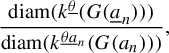 $$ \begin{align*} \dfrac{\text{diam}(k^{\underline{\theta}}(G(\underline{a}_n)))} {\text{diam}(k^{\underline{\theta}\underline{a}_n}(G(a_n)))}, \end{align*} $$
because of the relation
 $F^{\underline {\theta }\underline {a}_n} \circ k^{\underline {\theta }\underline {a}_n}= k^{\underline {\theta }} \circ f_{\underline {a}_n}$
applied to the domain
 $G(a_n)$
and the fact that
 $f_{\underline {a}_n}(G(a_n)) = G(\underline {a}_n)$
. Because the maps
 $k^{\underline {\theta }}$
,
 $\underline {\theta }\in \Sigma ^-$
, have a uniformly bounded derivative, there is a constant
 $C> 0$
such that the expansion term of
 $F^{\underline {\theta }\underline {a}_n}$
is less than
 $C \cdot \textrm {diam} (G(\underline {a}_n))$
and more than
 $C^{-1} \cdot \textrm {diam} (G(\underline {a}_n))$
.
However, because
 $h_n = h \circ (k^{\underline {\theta }})^{-1} \circ k^{\underline {\theta }} \circ f_{\underline {a}_n} = h \circ (k^{\underline {\theta }})^{-1} \circ F^{\underline {\theta }\underline {a}_n} \circ k^{\underline {\theta }\underline {a}_n}$
,
 $$ \begin{align*} DA_{h_n}^{-1} = Dh((k^{\underline{\theta}})^{-1}\circ F^{\underline{\theta}\underline{a}_n}(0))\cdot D(k^{\underline{\theta}})^{-1}(F^{\underline{\theta}\underline{a}_n}(0))\cdot DF^{\underline{\theta}\underline{a}_n}, \end{align*} $$
and
 $m( DA_{h_n}^{-1} )$
and
 $|DA_{h_n}^{-1}|$
are also controlled by
 $\textrm {diam} (G(\underline {a}_n))$
in the same way. Now, by Remark 3.7, the domain of interest of
 $h^{\underline {\theta }}$
on the relation
 $$ \begin{align*} h^{\underline{\theta}\underline{a}_n}_n= h_n \circ (k^{\underline{\theta a}_n})^{-1} = h \circ f_{\underline{a}_n} \circ (k^{\underline{\theta a}_n})^{-1} = h \circ (k^{\underline{\theta}})^{-1} \circ F^{\underline{\theta}\underline{a}_n} = h^{\underline{\theta}} \circ F^{\underline{\theta}\underline{a}_n} \end{align*} $$
is the set
 $F^{\underline {\theta }\underline {a}_n} \circ k^{\underline {\theta }\underline {a}_n}(G(a_n)) = k^{\underline {\theta }} (G(\underline {a}_n))$
, whose size is also controlled by
 $\textrm {diam} (G(\underline {a}_n))$
. Because the
 $(k^{\underline {\theta }})^{-1}$
vary continuously with
 $\underline {\theta }$
in a compact set, the maps
 $h^{\underline {\theta }}$
are
 $C^{1+\varepsilon }$
and, if we enlarge
 $C> 0 $
,
 $$ \begin{align*} \lvert Dh^{\underline{\theta}}(x)-Dh^{\underline{\theta}}(y) \rvert \le C \cdot |x-y|^{\varepsilon}, \end{align*} $$
for all
 $\underline {\theta } \in \Sigma ^{-}$
. Then, using Claim 3.9 with
 $\gamma = h^{\underline {\theta }}$
,
 $P = A_{h_n}$
,
 $Q = F^{\underline {\theta }\underline {a}_n}$
, and
 $X = k^{\underline {\theta }} (G(\underline {a}_n))$
and remembering that
 $A_{h_n} \circ {h_n}^{\underline {\theta }\underline {a}_n}(0) = 0$
and
 $D(A_{h_n} \circ {h_n}^{\underline {\theta }\underline {a}_n})(0) = {\textrm {Id}}$
, we have
 $$ \begin{align*} \Vert A_{h_n} \circ {h_n}^{\underline{\theta}\underline{a}_n}-{\textrm{Id}}\Vert = \Vert A_{h_n} \circ {h}^{\underline{\theta}} \circ F^{\underline{\theta}\underline{a}_n}-{\textrm{Id}}\Vert < C \cdot \text{diam}(G(\underline{a}_n))^{\varepsilon}. \end{align*} $$
The exponential decay of ratio
 $\mu $
is a consequence of Corollary 3.4.
The argument in the first paragraph of the previous proof gives us the following corollary.
Corollary 3.10 Given a Cantor set K, there is some constant
 $C> 0$
such that, for any
 $\underline {\theta } \in \Sigma ^-$
and
 $\underline {a} \in \Sigma ^{fin}$
,
 $$ \begin{align*} C^{-1} \,{\mathrm{diam}}(G(\underline{a})) \le \lvert DF^{\underline{\theta} \underline{a}} \rvert \le C \,{\mathrm{diam}} (G(\underline{a})). \end{align*} $$
3.3 Recurrent compact criterion
Given a pair of Cantor sets
 $K \text { and } K'$
, we are interested in finding configurations h and
 $h'$
such that
 $h(K)$
intersects
 $h'(K')$
. More importantly, we want to find a criterion under which this intersection is stable, that is, for small perturbations
 $\tilde {h},\,\tilde {h'}, \,\tilde {K},\,\tilde {K'}$
the sets
 $\tilde {h}(\tilde {K})$
and
 $\tilde {h'}(\tilde {K'})$
also have a non-empty intersection.
With these ideas in mind, for any pair of configurations
 $(h_a, h^{\prime }_{a'}) \in \mathcal {P}_a \times \mathcal {P}^{\prime }_{a'} $
we say that it is:
-
• linked whenever
$h_a(\overline {G(a)}) \cap h^{\prime }_{a'}(\overline {G(a')}) \neq \emptyset $
; -
• intersecting whenever
$h_a(K(a)) \cap h^{\prime }_{a'}(K'(a')) \neq \emptyset $
; -
• has stable intersections whenever
$\tilde {h}_{a}(\tilde {K}(a)) \cap \tilde {h'}_{a'}(\tilde {K'}(a')) \neq \emptyset $
for any pairs of Cantor sets
$(\tilde {K},\tilde {K'}) \in \Omega _\Sigma \times \Omega _{\Sigma '}$
in a small neighborhood of
$(K,K')$
and any configuration pair
$(\tilde {h}_{a},\tilde {h'}_{a'})$
that is sufficiently close to
$(h_a,h^{\prime }_{a'})$
in the
$C^{1+\varepsilon }$
topology at
$G(a) \cap \tilde {G}(a)$
and
$G(a') \cap \tilde {G}'(a')$
for some
$\varepsilon> 0$
.


It is better to work with
 $\mathcal {Q}$
, the quotient of
 $\mathcal {P} \times \mathcal {P}'$
by the diagonal action of
 $\textrm{Aff}(\mathbb {C})$
. We consider it equipped with the quotient topology. An element in
 $\mathcal {Q}$
, the equivalence class of a pair
 $(h,h') $
, denoted by
 $[h,h']$
, is called a relative configuration or, as mentioned sometimes, a relative positioning of the pair of Cantor sets. Because the action of the affine group preserves the linking, intersecting, or stable intersection of a pair of configurations, these notions are defined for relative configurations too. Also, we can define for any pair in
 $\mathcal {P} \times \mathcal {P}'$
and any pair of words
 $(\underline {a},\underline {a}') \in \Sigma ^{fin} \times {\Sigma '}^{fin}$
a renormalization operator
 $$ \begin{align*} {\mathcal{T}}_{\underline{a},\underline{a}'} (h,h') : = (T_{\underline{a}}(h),T_{\underline{a}'}(h')). \end{align*} $$
For the same reasons as above, it can also be defined over
 $\mathcal {Q}$
. Also, we can allow one of the words
 $\underline {a}$
or
 $\underline {a}'$
to be void. In that case, the operator only acts at the non-trivial coordinate, for example
 $$ \begin{align*} {\mathcal{T}}_{\emptyset,\underline{a}'} (h,h')=(h,T_{\underline{a}'}(h')). \end{align*} $$
Although we considered in
 $\mathcal {Q}$
the quotient topology coming from the
 $C^r$
,
 $r>1$
, topology of
 $\mathcal {P}\times \mathcal {P}'$
, in the next lemma, we are going to consider the topology coming from the
 $C^1$
topology in
 $\mathcal {P}\times \mathcal {P}'$
. This is just a practical simplification. Under this context, we have the following.
Lemma 3.11 A relative configuration
 $[h_0, h^{\prime }_0]$
is intersecting if, and only if, there is a relatively compact sequence (in the
 $C^1$
topology of
 $\mathcal {Q}$
) of relative configurations
 $[h_n,h^{\prime }_n]$
obtained inductively by applying a renormalization operator that acts trivially on one of the coordinates of the equivalence class.
Proof. If
 $h_0(K)$
and
 $h^{\prime }_0(K')$
are intersecting at a point
 $q= h_0(p) = h^{\prime }_0 (p')$
, (
 $p \in K $
and
 $p' \in K'$
), consider the sequences
 $H(p) = (a_0, a_1, \ldots ) \in \Sigma $
and
 $H'(p)=(a^{\prime }_0,a^{\prime }_1, \ldots ) \in \Sigma '$
, where H and
 $H'$
are the homeomorphisms defined in §2.1. We can construct a sequence of pairs of configurations
 $(h_n, h^{\prime }_n)$
, obtained by successively renormalizing by the functions
 $f_{(a_{i},a_ {i+1})}$
and
 $f_{(a^{\prime }_{j},a^{\prime }_{j+1})}$
,
 $i,\, j \ge 0$
, chosen in a careful order such that the ratio of diameters of the sets
 $G(\underline {b}_n)$
and
 $G(\underline {b}^{\prime }_n)$
are bounded away from
 $0$
and
 $\infty $
, where
 $(h_n,h^{\prime }_n) = (h\circ f_{\underline {b}_n}, h' \circ f_{\underline {b}^{\prime }_n})$
,
 $\underline {b}_n=(a_0,\,\ldots ,\,a_{r_n})$
, and
 $\underline {b}^{\prime }_n=(a^{\prime }_0,\,\ldots ,\,a^{\prime }_{r^{\prime }_n})$
(notice that
 $r_n \le n$
and
 ${r^{\prime }_n \le n}$
).
Indeed, if
 $\underline {a}_n = (a_0,\,\ldots ,a_n)$
, by equation (3.2) of Lemma 3.1 and Corollary 3.2,
 $\text {diam}(G(\underline {a}_n))$
is comparable to
 $\text {diam}(G(\underline {a}_{n-1}))$
. Therefore, if we choose carefully which coordinate to act trivially, we can keep the ratios bounded.
Finally, such pairs of configurations are always intersecting, because the point q belongs to both their images. Using Claim 3.9, with
 $\gamma = h_0 \circ (k^{\underline {\theta }})^{-1}$
,
 $X = G(\underline {b}_n)$
,
 $P = A_{h_n}$
,
 $Q = F^{\underline {\theta }\underline {b}_n}$
; and with
 $\gamma = h^{\prime }_0\circ (k^{\underline {\theta }'})^{-1}$
,
 $X = G(\underline {b}^{\prime }_n)$
,
 $P = A_{h_n}$
,
 $Q = F^{\underline {\theta }'\underline {b}^{\prime }_n}$
, in a similar way as done in the proof of Lemma 3.8, it follows that the sequence
 $[h_n, h^{\prime }_n]$
is relatively compact in
 $\mathcal {Q}$
.
However, let
 $[h_n,h^{\prime }_n]$
be such a relatively compact sequence. We can consider
 $(h_n, h_n') = \mathcal {T}_{\underline {b}_n,\underline {b}^{\prime }_n} (h_0,h^{\prime }_0)$
. Then
 $(h_n,h^{\prime }_n)$
is linked, because if it was not, the distance between the images of their scaled versions,
 $(A_{h_n}\circ h_n, A_{h_n}\circ h^{\prime }_n )$
, would go to infinity as
 $n \rightarrow \infty $
. Hence, choosing points
 $p_n \in h_n(K) \subset h_0(K)$
and
 $p^{\prime }_n \in h^{\prime }_n(K') \subset h^{\prime }_0(K')$
, it follows that
 $\lim _{n \rightarrow \infty } p_n = p = \lim _{n \rightarrow \infty } p^{\prime }_n $
, because the diameter of the sets
 $h_n(K)$
and
 $h^{\prime }_n(K')$
converge exponentially to
 $0$
as
 $n \rightarrow \infty $
, as they are controlled by
 $\text {diam}(G(\underline {b}_n))$
and
 $\text {diam} (G'(\underline {b}^{\prime }_n))$
, respectively, and they are always linked. Because K and
 $K'$
are closed,
 $p \in h_0(K) \cap h^{\prime }_0(K') \neq \emptyset $
as we wanted to show.
This lemma is very important in finding a criterion for stable intersection in Cantor sets. To do it, we will work with the space of relative affine configurations of limit geometries.
Definition 3.4 The space of relative affine configurations of limit geometries will be denoted by
 $\mathcal {C}$
. It is the quotient of
 $\mathcal {A} \times \mathcal {A}'$
by the action of the affine group by composition on the left, that is,
 $((A,\underline {\theta }), (A',\underline {\theta }')) \mapsto ((B \circ A,\underline {\theta }), (B \circ A',\underline {\theta }'))$
, where B ranges in
 $\textrm{Aff}(\mathbb {C})$
.
The concepts of linking, intersection, and stable intersection were well defined for pairs of affine configurations of limit geometries, and again, because they are invariant by the action of
 $\textrm{Aff}(\mathbb {C})$
, they are also defined for relative configurations in
 $\mathcal {C}$
. Also, because the renormalization operator acts by multiplication on the right on
 $(A,\underline {\theta })$
, its action commutes with the multiplication on the left by affine transformations and so it can be naturally defined on
 $\mathcal {C}$
. This space can be identified with
 $\Sigma ^- \times {\Sigma '}^{-} \times \textrm{Aff}(\mathbb {C})$
by the identification
 $[(A, \underline {\theta }), (A', \underline {\theta }')] \equiv (\underline {\theta }, \underline {\theta }', {A}^{-1} \circ A')$
, and in this manner, the topology on
 $\mathcal {C}$
is the product topology on
 $\Sigma ^- \times {\Sigma '}^{-} \times \textrm{Aff}(\mathbb {C})$
.
Definition 3.5 (Recurrent compact set)
Let
 $\mathcal {L}$
be a compact set in
 $\mathcal {C}$
. We say that
 $\mathcal {L}$
is recurrent if for any relative affine configuration of limit geometries
 $v \in \mathcal {L}$
, there are words
 $\underline {a}$
,
 $\underline {a}'$
such that
 $u=\mathcal {T}_{\underline {a},\underline {a'}} (v) $
satisfies
 $u \in {\textrm {int}}\,\mathcal {L}$
.
If such a renormalization can be done using words
 $\underline {a}$
and
 $\underline {a}'$
such that their total size combined is equal to one, we say that such a set is immediately recurrent.
Theorem 3.12 The following properties are true.
-
(1) Every recurrent compact set is contained in an immediately recurrent compact set.
-
(2) Given a recurrent compact set
$\mathcal {L}$
(respectively immediately recurrent) for g,
$g'$
, for any
$(\tilde {g},\tilde {g}')$
in a small neighborhood of
$(g,g') \in \Omega _{\Sigma } \times \Omega _{{\Sigma }'}$
, we can choose base points
$\tilde {c}_a \in \tilde {G}(a) \cap \tilde {K}$
and
$\tilde {c}_{a'} \in \tilde {G}(a') \cap \tilde {K}'$
respectively close to the pre-fixed
$c_a$
and
$c_{a'}$
, for all
$a \in \mathbb {A}$
and
$a' \in \mathbb {A'}$
, in a manner that
$\mathcal {L}$
is also a recurrent compact set for
$\tilde {g}$
and
$\tilde {g}'$
. -
(3) Any relative configuration contained in a recurrent compact set has stable intersections.


Proof. (1) We remember that
 $\mathcal {A}$
is a metric space, so for every point v of the recurrent compact set
 $\mathcal {L}$
, there is a closed ball around v that is carried by a renormalization (given by a pair of words
 $\underline {a}^{v}, \, {\underline {a}'}^{v}$
) into the interior of
 $\mathcal {L}$
. Because this set is compact and by continuity of the renormalization operator, there is a finite number N of compact sets (balls)
 $\mathcal {L}^{i}$
whose union covers
 $\mathcal {L}$
and associated pair of words
 $(\underline {a}^{i},{\underline {a}'}^{i})$
for
 $1 \leq i \leq N$
such that
 $\mathcal {L}^i$
is carried into the interior of
 $\mathcal {L}$
by the renormalization associated to the pair
 $(\underline {a}^{i},{\underline {a}'}^{i})$
. Now, consider for every such pair, all the pairs of words
 $(\underline {b}^{i,j},{\underline {b}'}^{i,j})$
such that
 $\underline {b}^{i,j}$
is a subword of
 $\underline {a}^{i}$
and
 ${\underline {b}'}^{i,j}$
is a subword of
 ${\underline {a}'}^{i}$
. We construct an immediately recurrent Cantor set
 $\mathcal {L}'$
in the following way.
First, we choose one of the two pairs
 $(\underline {b}^{i,j_1},{\underline {b}'}^{i,j_1})$
with total size
 $1$
sharing the same beginning with
 $(\underline {a}^i,{\underline {a}'}^i)$
and write
 $(\underline {b}^{i,\overline {j_1}},{\underline {b}'}^{i,\overline {j_1}})$
as the word pair that needs to be concatenated to
 $(\underline {b}^{i,j_1},{\underline {b}'}^{i,j_1})$
to result in
 $(\underline {a}^{i},{\underline {a}'}^{i})$
. By continuity, there is a compact set
 $\mathcal {L}^{i(1)}$
such that
 ${\textrm {int}}\, \mathcal {L}^{i(1)} \supset T_{(\underline {b}^{i,j_1},{\underline {b}'}^{i,j_1})} \mathcal {L}^i $
and
 $T_{(\underline {b}^{i,\overline {j_1}},{\underline {b}'}^{i,\overline {j_1}})} \mathcal {L}^{i(1)} \subset {\textrm {int}}\, \mathcal {L} $
. This can be done in the same manner the sets
 $\mathcal {L}^i$
were constructed just above.
Then we inductively construct a sequence of compact sets
 $\mathcal {L}^{i(k)}$
,
 $k=1, \ldots , m$
such that for each
 $\mathcal {L}^{i(k)}$
, there is a renormalization by a pair of words of total size one that carries it into
 ${\textrm {int}}\, \mathcal {L}^{i(k+1)}$
for
 $k= 1, \ldots , m-1$
and carries
 $\mathcal {L}^{i(m)}$
into
 ${\textrm {int}}\, \mathcal {L}$
, where m is the total size of
 $(\underline {a}^i,{\underline {a}'}^i)$
. Then, taking
 $\mathcal {L}' = \bigcup _{i(k)} \mathcal {L}^{i(k)}$
, we have an immediately recurrent compact set.
(2) Using the decomposition
 $\mathcal {L} = \cup ^{N}_{i=1} \mathcal {L}_i$
, described in the previous argument, it is enough to show that for any
 $\varepsilon>0$
, there is
 $\delta> 0$
such that, for any pair
 $(\tilde {g}, \tilde {g}')$
in
 $U_{K,\delta } \times U_{K',\delta } $
, the renormalization operators associated to the words
 $\underline {a}^{i} \text { and } {\underline {a}'}^{i}$
,
 $i=1, \ldots , N$
, denoted by
 $\tilde {\mathcal {T}}_{\underline {a}^{i},{\underline {a}'}^{i}}=(\tilde {T}_{\underline {a}^{i}},\tilde {T}_{{\underline {a}'}^{i}})$
, satisfy
 $ \Vert \tilde {\mathcal {T}}-\mathcal {T}\Vert < \varepsilon $
.
These operators are obtained by composition of a finite number of operators arising from pairs of words of total size one, and so we need only to show that for any
 $\varepsilon '>0$
, a
 $\delta> 0$
can be found such that
 $|T_{(a,b)}-\tilde {T}_{(a,b)}|<\varepsilon '$
and
 $|T_{(a',b')}-\tilde {T}_{(a',b')}|<\varepsilon '$
for all pairs
 $(a,b) \in B$
and
 $(a',b') \in B'$
, or precisely, by Lemma 3.6, that for any
 $\underline {\theta } \in \Sigma ^-$
and
 $\theta _1 \in \mathbb {A}$
,
 $|F^{\underline {\theta }\theta _1} -\tilde {F}^{\underline {\theta }\theta _1} | < \varepsilon '$
, and its analogous version for
 $K' \text { and } \tilde {K}'$
. However, as seen in Lemma 3.6,
 $F^{\underline {\theta }\theta _1}=k^{\underline {\theta }} \circ f_{\theta _0,\theta _1} \circ (k^{\underline {\theta }\theta _1})^{-1}$
, and we need only to show that the values of all the functions and their derivatives above at a fixed point x do not change much when considering its
 $ \tilde {K} $
version. This is was done in Lemma 3.5.
(3) Given a recurrent compact set
 $\mathcal {L}$
relative to a pair of Cantor sets K and
 $K'$
, its image under
 $$ \begin{align*} I : \mathcal{C} & \to \mathcal{Q} \\ [(A,\underline{\theta}),(A',\underline{\theta}')] & \mapsto [A \circ k^{\underline{\theta}},A' \circ k^{\underline{\theta}'}] \end{align*} $$
is also a compact set, because this association is continuous. In what follows, whenever we work with the set
 $\mathcal {L}$
in the context of
 $\mathcal {Q}$
, we are referring to the set
 $I(\mathcal {L})$
.
In this sense, any pair
 $(A\circ k^{\underline {\theta }},{A'}\circ {k}^{\underline {\theta }'})$
representing a relative affine configuration of limit geometries v belonging to
 $\mathcal {L}$
is intersecting, because, considering it a part of an immediately recurrent compact set, one can construct a sequence as in the hypothesis of Lemma 3.11. In light of the previous item, this implies that
 $A \circ \tilde {k}^{\underline {\theta }}$
and
 $A' \circ \tilde {{k}}^{\underline {\theta }'}$
also represent intersecting configurations for a pair of Cantor sets
 $(\tilde {K},\tilde {K'})$
sufficiently close to
 $(K,K')$
.
Thus, it is enough to show that, for any pair of Cantor sets
 $(K,K')$
that has a recurrent compact set
 $\mathcal {L}$
and a configuration pair
 $v \in \mathcal {L}$
represented by
 $[(A,\underline {\theta }),(A',\underline {\theta }')]$
, if
 $h : {\textrm {Im}}(A \circ k^{\underline {\theta }}) \to \mathbb {C}$
and
 $h' : {\textrm {Im}}(A \circ k^{\underline {\theta }'}) \to \mathbb {C}$
are embeddings
 $C^{1+\varepsilon }$
close to the identity, then
 $h \circ A \circ k^{\underline {\theta }}$
and
 $h' \circ A' \circ k^{\underline {\theta }'}$
are also intersecting.
To accomplish this, we will construct a relatively compact sequence of relative configurations
 $[h_n,h^{\prime }_n] \in \mathcal {Q}$
, with
 $[h_0,h^{\prime }_0] = [h \circ A \circ k^{\underline {\theta }}, h' \circ A' \circ k^{\underline {\theta }'}]$
, obtained inductively by renormalization. If we have such a sequence, the result follows from Lemma 3.11 again. We are going to represent each equivalence class
 $[h_n, h^{\prime }_n]$
by its representative that is scaled on the first coordinate (remember Definition 3.3). We are also interested on how ‘far’ each term of this sequence is from being in
 $\mathcal {L}$
, thus we write
 $$ \begin{align*}[h_n,h^{\prime}_n] = [ \eta_n \circ k^{\underline{\theta}(n)}, \eta^{\prime}_n \circ B_n \circ k^{\underline{\theta}'(n)} ]\end{align*} $$
for some limit geometries
 $$ \begin{align*}\underline{\theta}(n) &= (\ldots,\, \theta_{-n},\,\ldots,\, \theta_0, \,\ldots,\,\theta_{r_n})\in \Sigma^- \quad \text{ and }\\ \underline{\theta}'(n) &= (\ldots,\, \theta^{\prime}_{-n},\,\ldots,\, \theta^{\prime}_0, \,\ldots, \,\theta^{\prime}_{r^{\prime}_n} ) \in {\Sigma'}^-\end{align*} $$
and in what follows, we will show that these choices can be done so that
 $\eta _n$
and
 $\eta ^{\prime }_n$
are maps
 $C^1$
close to the identity in their domains,
 $ k^{\underline {\theta }(n)}(G(\theta _{n_r})) $
and
 $ k^{\underline {\theta }'(n)}(G(\theta _{n^{\prime }_r})) $
, respectively,
 $B_n \in \textrm{Aff}(\mathbb {C})$
and
 $ [ k^{\underline {\theta }(n)}, B_n \circ k^{\underline {\theta }'(n)} ] \in \textrm{int}\, \mathcal {L}$
for all
 $n \ge 1$
. If this is the case for all
 $n \ge 1$
, then the sequence is relatively compact and the proof is complete.
To prove the estimates for
 $\eta _n$
and
 $\eta ^{\prime }_n$
for large values of n, we are going to use Claim 3.9 many times. For
 $n=0$
, we make
 $\underline {\theta }(0)=\underline {\theta }$
and
 $\underline {\theta }'(0)=\underline {\theta }'$
, and so
 $\eta _0$
is the perturbed part of the scaled version of
 $h \circ A \circ k^{\underline {\theta }}$
relative to
 $k^{\underline {\theta }(0)} = k^{\underline {\theta }}$
; in other words, if
 $A(z)=\alpha \cdot z + \beta $
and we denote
 $\Gamma _0(z)=h(\beta )+Dh(\beta )\cdot (z-\beta )$
,
 $$ \begin{align*} \eta_0 = A^{-1} \circ \Gamma_0^{-1} \circ h \circ A. \end{align*} $$
Moreover, if we denote
 $A'(z)=\alpha ' \cdot z+ \beta '$
and
 $\Gamma ^{\prime }_0(z)=h'(\beta ')+Dh'(\beta ')\cdot (z-\beta ')$
, then
 $$ \begin{align*} \eta^{\prime}_0 \circ B_0 = A^{-1} \circ {\Gamma^{\prime}_0}^{-1} \circ h' \circ A'. \end{align*} $$
It follows from continuity that if h and
 $h'$
are sufficiently close to the identity in their domains, then
 $\eta _0$
is close to the identity and
 $\eta ^{\prime }_0 \circ B_0$
is close to
 $A^{-1} \circ A'$
.
Therefore, for
 $n=0$
, we make
 $\underline {\theta }(0)=\underline {\theta }$
,
 $\underline {\theta }'(0)=\underline {\theta }'$
,
 $B_0=A^{-1} \circ A'$
,
 $\eta _0 = A^{-1} \circ \Gamma _0^{-1} \circ h \circ A$
, and
 $\eta ^{\prime }_0 = A^{-1} \circ {\Gamma ^{\prime }_0}^{-1} \circ h' \circ A$
; and the base of our construction is complete.
Now consider a decomposition of the recurrent compact set
 $\mathcal {L} = \cup \mathcal {L}^i$
as done in item
 $(1)$
and fix a set of renormalizations
 $T_{\underline {a}^i,{\underline {a}'}^i}$
that carries each
 $\mathcal {L}^i$
to the interior of
 $\mathcal {L}$
. We can find a
 $\delta>0$
such that the distance of any
 $T_{\underline {a}^i,{\underline {a}'}^i}(v),\, v \in \mathcal {L}^i$
to the boundary of
 $\mathcal {L}$
is bigger than
 $\delta $
. The idea is to use the series of renormalizations that worked for
 $[A\circ k^{\underline {\theta }},A'\circ k^{\underline {\theta }'} ]$
and do small adaptations along the way.
Let us show how to go from
 $[h_n, h^{\prime }_n]$
to
 $[h_{n+1}, h^{\prime }_{n+1}]$
. If
 $$ \begin{align*} [h_n,h^{\prime}_n] = [ \eta_n \circ k^{\underline{\theta}(n)}, \eta^{\prime}_n \circ B_n \circ k^{\underline{\theta}'(n)} ], \end{align*} $$
we choose
 $\underline {a}(n) = (\theta _{r_n},\, \ldots ,\, \theta _{r_{n+1}} ) \in \Sigma ^{fin}$
and
 $\underline {a}'(n) = (\theta ^{\prime }_{r^{\prime }_n},\, \ldots ,\, \theta ^{\prime }_{r^{\prime }_{n+1}} )\in {\Sigma '}^{fin}$
among the words fixed in the previous paragraph such that
 $$ \begin{align*} \mathcal{T}_{\underline{a}(n),\underline{a}'(n)} ( k^{\underline{\theta}(n)}, B_n \circ k^{\underline{\theta}'(n)} ) \in \textrm{int}(\mathcal{L}) \end{align*} $$
and make
 $$ \begin{align*} [h_{n+1}, h^{\prime}_{n+1}] = \mathcal{T}_{\underline{a}(n),\underline{a}'(n)} [h_n, h^{\prime}_n]. \end{align*} $$
We need now to explain how the choices of
 $\underline {\theta }(n+1)$
,
 $\eta _{n+1}$
,
 $\underline {\theta }'(n+1)$
,
 $B_{n+1}$
,
 $\eta ^{\prime }_{n+1}$
must be made. Some of them are automatic, for example, we make
 $\underline {\theta }(n+1) = \underline {\theta }(n)\underline {a}(n)$
and
 $\underline {\theta }'(n+1) = \underline {\theta }'(n)\underline {a}'(n)$
. Writing
 $\underline {b}(n) = \underline {a}(0) \underline {a}(1) \cdots \underline {a}(n)$
and
 $\underline {b}'(n) = \underline {a}'(0) \underline {a}'(1) \cdots \underline {a}'(n)$
, it follows by induction on n, having in mind Remark 3.7, that
 $$ \begin{align} [h_{n+1}, h^{\prime}_{n+1}] & = \mathcal{T}_{\underline{b}(n), \underline{b}'(n)} [h_0, h^{\prime}_0] \nonumber\\ & = [h \circ A \circ k^{\underline{\theta}} \circ f_{\underline{b}(n)}, h' \circ A' \circ k^{\underline{\theta}'} \circ f_{\underline{b}'(n)}] \nonumber\\ & = [ h \circ A \circ F^{\underline{\theta}\, \underline{b}(n)} \circ k^{\underline{\theta}(n + 1)}, h' \circ A' \circ F^{\underline{\theta}' \, \underline{b}'(n)} \circ k^{\underline{\theta}'(n + 1)} ]. \end{align} $$
We recall that
 $F^{\underline {\theta }\, \underline {b}(n)}$
and
 $F^{\underline {\theta }'\, \underline {b}'(n)}$
are the affine maps that help us do calculations with renormalizations that were defined in Remark 3.7. Because we want the first coordinate of
 $$ \begin{align*} [ \eta_{n+1} \circ k^{\underline{\theta}(n + 1)}, \eta^{\prime}_{n + 1} \circ B_{n + 1} \circ k^{\underline{\theta}'(n + 1)} ] ( = [h_{n+1},h^{\prime}_{n+1}] ) \end{align*} $$
to be a scaled configuration,
 $\eta _{n+1}$
must satisfy:
 $$ \begin{align*} \eta_{n+1} = (F^{\underline{\theta}\, \underline{b}(n)})^{-1} \circ A^{-1} \circ \Gamma_{n}^{-1} \circ h \circ A \circ F^{\underline{\theta}\, \underline{b}(n)}, \end{align*} $$
where
 $ A \circ F^{\underline {\theta }\, \underline {b}(n)} (z) = \alpha _n \cdot z + \beta _n$
,
 $\alpha _n \in \mathbb {C}^*$
, and
 $\beta _n \in \mathbb {C}$
, and
 $\Gamma _{n} \in \textrm{Aff}(\mathbb {C}^2)$
is an affine map defined as
 $\Gamma _{n}(z) = Dh(\beta _n)(z-\beta _n) + h(\beta _n) $
.
By Claim 3.9, making
 $ P = (F^{\underline {\theta }\, \underline {b}(n)})^{-1} \circ A^{-1} \circ \Gamma _{n}^{-1}$
,
 $Q = A \circ F^{\underline {\theta }\, \underline {b}(n)}$
,
 $\gamma = h$
,
 $p = \beta _n$
, and
 $$ \begin{align*}X = (A \circ F^{\underline{\theta}\, \underline{b}(n)})(k^{\underline{\theta}(n+1)}(G(\theta_{r_{n+1}}))) = A( k^{\underline{\theta}}(G (\underline{b}(n) ) )),\end{align*} $$
it follows that
 $\eta _{n+1}$
is
 $C \cdot {\textrm {diam}}(X)\, C^1$
-close to the identity in its domain
 $k^{\underline {\theta }(n+1)}(G(\theta _{r_{n+1}}))$
, if n is sufficiently large. Notice that
 ${\textrm {diam}}(X)$
decays exponentially with n, so for large n, the map
 $\eta _{n+1}$
is very close to the identity. For small values, we can make h sufficiently close to the identity so that the same conclusion is true.
The construction of the terms in the second entry is where the proof really happens. Define the map
 $T_n : \mathbb {C} \to \mathbb {C}$
by
 $$ \begin{align*} T_n := (F^{\underline{\theta}\, \underline{b}(n)})^{-1} \circ A^{-1} \circ {\Gamma}_{n}^{-1} \circ h' \circ A' \circ F^{\underline{\theta}'\, \underline{b}'(n)}. \end{align*} $$
Again, because the first coordinate of
 $[ \eta _{n+1} \circ k^{\underline {\theta }(n + 1)}, \eta ^{\prime }_{n + 1} \circ B_{n + 1} \circ k^{\underline {\theta }'(n + 1)} ]$
is scaled, by equation (3.11),
 $$ \begin{align} \eta^{\prime}_{n+1}\circ B_{n+1} = T_n. \end{align} $$
The key is to realize that although
 $T_n$
is fixed after the choices of
 $\underline {a}_n$
and
 $\underline {a}^{\prime }_n$
, we can choose the maps
 $\eta ^{\prime }_{n+1}$
and
 $B_{n+1}$
in a smart way so that they have the properties previously stated, which means that
 $\eta ^{\prime }_{n+1}$
is close to the identity and
 $[k^{\underline {\theta }(n+1)}, B_{n+1} \circ k^{\underline {\theta }'(n+1)}] \in \textrm{int} \, \mathcal {L}$
.
A naive idea is to make
 $B_{n+1} = (F^{\underline {\theta }(n)\,\underline {a}(n)})^{-1} \circ B_n \circ F^{\underline {\theta }'(n)\,\underline {a}'(n)} $
, because then
 $$ \begin{align*} [k^{\underline{\theta}(n+1)}, B_{n+1} \circ k^{\underline{\theta}'(n+1)}] = \mathcal{T}_{\underline{a}(n), \underline{a}'(n)}[k^{\underline{\theta}(n)}, B_{n} \circ k^{\underline{\theta}'(n)}] \in \textrm{int}\, \mathcal{L}. \end{align*} $$
However, this choice would not work, because we would lose control of the distance of
 $\eta ^{\prime }_{n+1}$
to the identity. If we make this choice of
 $B_{n+1}$
for every
 $n \ge 0$
, then, following equation (3.11), one could prove that
 $$ \begin{align*} \eta^{\prime}_{n+1} = (F^{\underline{\theta}\, \underline{b}(n)})^{-1} \circ A^{-1} \circ {\Gamma}_{n}^{-1} \circ h' \circ A \circ F^{\underline{\theta}\, \underline{b}(n)}. \end{align*} $$
The composition of terms to the left-hand side of
 $h'$
yields an affine map that is an expansion by a factor comparable to
 $\mu ^{n}$
, where
 $\mu $
is the expanding factor of g. If
 $h' = {\textrm {Id}} + \omega $
for some
 $\omega \in \mathbb {C}$
close to
 $0$
, then the distance of
 $\eta ^{\prime }_{n+1}$
to the identity would be exponentially big, also depending on n.
Even so, a small translation is sufficient to make the construction work. So we write
 $$ \begin{align*} \tilde{B}_{n+1} := (F^{\underline{\theta}(n)\,\underline{a}(n)})^{-1} \circ B_n \circ F^{\underline{\theta}'(n)\,\underline{a}'(n)} \end{align*} $$
instead and use it as an auxiliary map for the construction of
 $B_{n+1}$
. It is important to see that in our inductive construction below, the derivatives of
 $B_{n+1}$
and
 $\tilde {B}_{n+1}$
are the same, therefore, by induction,
 $$ \begin{align} D\tilde{B}_{n+1} = DB_{n+1} = D((F^{\underline{\theta}\, \underline{b}(n)})^{-1} \circ A^{-1} \circ A' \circ F^{\underline{\theta}'\, \underline{b}'(n)}). \end{align} $$
If
 $ A' \circ F^{\underline {\theta }'\, \underline {b}'(n)} (z) = \alpha ^{\prime }_n \cdot z + \beta ^{\prime }_n$
, the derivative of
 $T_n$
at zero is equal to
 $$ \begin{align*} DT_n(0) & = (DF^{\underline{\theta}\, \underline{b}(n)})^{-1} \cdot DA^{-1} \cdot Dh(\beta_n)^{-1} \cdot Dh'(\beta^{\prime}_n) \cdot DA' \cdot DF^{\underline{\theta}'\, \underline{b}'(n)} \\ & = \alpha_n^{-1}\cdot Dh(\beta_n)^{-1} \cdot Dh'(\beta^{\prime}_n) \cdot \alpha^{\prime}_n. \end{align*} $$
Hence, because
 $\alpha _n^{-1} \cdot \alpha ^{\prime }_n = D((F^{\underline {\theta }\, \underline {b}(n)})^{-1} \circ A^{-1} \circ A' \circ F^{\underline {\theta }'\, \underline {b}'(n)}) = D\tilde {B}_{n+1}$
is bounded, as
 $$ \begin{align*} [k^{\underline{\theta}(n+1)}, \tilde{B}_{n+1} \circ k^{\underline{\theta}'(n+1)}] = \mathcal{T}_{\underline{a}(n),\underline{a}'(n)} ( k^{\underline{\theta}(n)}, B_n \circ k^{\underline{\theta}'(n)} ) \in \textrm{int}(\mathcal{L}),\end{align*} $$
 $DT_n(0)$
is
 $C' \cdot \lVert Dh^{-1}-{\textrm {Id}} \rVert \cdot \lVert Dh'-{\textrm {Id}} \rVert $
close to
 $D\tilde {B}_{n+1}$
for some constant
 $C'> 0 $
depending on
 $\mathcal {L}$
.
Under this notation,
 $B_{n+1} \in \textrm{Aff}(\mathbb {C})$
is defined as
 $$ \begin{align*} B_{n+1}(z):= D\tilde{B}_{n+1} \cdot z + T_n(0). \end{align*} $$
To show that it is
 $\delta $
close to
 $\tilde {B}_{n+1}$
, we must estimate
 $\lvert T_n(0) - \tilde {B}_{n+1}(0) \rvert $
. We use Claim 3.9 again.
First, making
 $P = (F^{\underline {\theta }\, \underline {b}(n)})^{-1} \circ A^{-1}$
,
 $Q = A' \circ F^{\underline {\theta }'\, \underline {b}'(n)}$
,
 $\gamma = \Gamma _n^{-1} \circ h'$
,
 $p = \beta ^{\prime }_n$
, and
 $$ \begin{align*} X = (A' \circ F^{\underline{\theta}'\, \underline{b}'(n)})(k^{\underline{\theta}'(n+1)}(G(\theta^{\prime}_{r^{\prime}_{n+1}}))) = A'( k^{\underline{\theta}'}(G (\underline{b}'(n) ) )), \end{align*} $$
it follows that
 $T_n(0)$
is
 $C'' \cdot {\textrm {diam}} (X)^\varepsilon $
close to
 $P \circ \Gamma \circ Q (0)$
for large values of n, where
 $C''> 0$
is a constant depending on h and
 $h'$
,
 $$ \begin{align*}\Gamma = \Gamma_n^{-1} \circ \Gamma^{\prime}_n \quad\text{ and }\quad \Gamma^{\prime}_n(z) = Dh'(\beta^{\prime}_n)(z- \beta^{\prime}_n) + h'(\beta^{\prime}_n).\end{align*} $$
At the same time,
 $\Gamma $
is close to the identity, because h and
 $h'$
are. Proceeding in the same manner we did to estimate
 $DT_n(0)$
, we find
 $$ \begin{align*} \lvert T_n(0) - \tilde{B}_{n+1}(0) \rvert &\le \lvert T_n(0) - P \circ \Gamma \circ Q (0) \rvert + \lvert P \circ \Gamma \circ Q (0) - \tilde{B}_{n+1}(0) \rvert \\ & \le C'' \cdot {\textrm{diam}} (X)^\varepsilon + C' \cdot \lVert \Gamma_n^{-1} - {\textrm{Id}} \rVert \cdot \lVert \Gamma^{\prime}_n - {\textrm{Id}} \rVert , \end{align*} $$
and consequently, this difference can be made smaller than
 $\delta $
if n is sufficiently large and h and
 $h'$
are sufficiently close to the identity. For small values of n, the same conclusion is true by continuity if we make h and
 $h'$
sufficiently close to the identity.
Finally, we need only to check the estimate on
 $\eta _{n+1}'$
. By equation (3.12), we can write this function as
 $P \circ \gamma \circ Q$
, where
 $P = (F^{\underline {\theta }\, \underline {b}(n)})^{-1} \circ A^{-1} \circ \Gamma _n^{-1}$
,
 $\gamma = h'$
,
 $Q = A' \circ F^{\underline {\theta }'\, \underline {b}'(n)} \circ B_{n+1}^{-1}$
and the domain of
 $\gamma $
is
 $$ \begin{align*} X = A' \circ F^{\underline{\theta}'\, \underline{b}'(n)} (k^{\underline{\theta}'(n+1)}(G(\theta^{\prime}_{r^{\prime}_{n+1}}))). \end{align*} $$
Observe that, because of Corollary 3.10, the affine map P expands distances by a factor comparable to the inverse of
 ${\textrm {diam}}(G(\underline {b}'(n)))$
– we are considering the maps A and
 $A'$
fixed here. Moreover, because
 $D\tilde {B}_{n+1} = DB_{n+1}$
is bounded away from zero and infinity, as
 $\mathcal {L}$
is compact (remember that
 $\textrm{Aff}(\mathbb {C})$
contains only invertible transformations),
 $Q^{-1}$
also expand distances by a factor comparable to the inverse of
 ${\textrm {diam}}(G(\underline {b}'(n)))$
, because
 $DP \cdot DQ$
is close to the identity by equation (3.13). The diameter of X is also comparable to these values.
Making
 $p = \beta ^{\prime }_n$
, the map
 $\eta ^{\prime }_{n+1}$
is thus
 $C \cdot {\textrm {diam}} (X)^{\varepsilon } $
close to
 $P \circ \Gamma \circ Q$
, where
 $\Gamma = D\gamma (p)(z - p) + \gamma (p)$
. However, the definition of these maps imply that
 $P \circ \gamma \circ Q = T_n \circ B^{-1}_{n+1}$
. Hence,
 $P \circ \Gamma \circ Q$
is an affine transformation that has derivative equal to
 $$ \begin{align*} D(P \circ \gamma \circ Q) (Q^{-1}(p)) = D( T_n \circ B^{-1}_{n+1})(Q^{-1}(p)) & = DT_n(B^{-1}_{n+1} \circ Q^{-1}(p)) \cdot DB^{-1}_{n+1}\\ & = DT_n(0) \cdot DB^{-1}_{n+1}, \end{align*} $$
which is close to the identity because
 $DB_{n+1}^{-1}$
is bounded and has
 $ B_{n+1}(0) = T_n(0)$
as a fixed point. This implies that
 $\eta ^{\prime }_{n+1}$
is close to the identity for large n. For small n, the result follows by continuity as done many times before.
Remark 3.13. We remark that the sequence of renormalizations
 $\mathcal {T}_{\underline {a}(n), \underline {a}'(n)}$
constructed above for a pair
 $(h, h')$
close to the identity is not necessarily equal to the sequence of renormalizations constructed for
 $(h, h') = ({\textrm {Id}}, {\textrm {Id}})$
. Notice that the choice of the maps
 $B_{n+1}$
has an influence on the choice of the pair
 $(\underline {a}(n + 1), \underline {a}'(n + 1))$
and may make it different from the one working for
 $(h, h') = ({\textrm {Id}}, {\textrm {Id}})$
. This may happen because the relative configurations
 $[k^{\underline {\theta }(n)}, \tilde {B}_n \circ k^{\underline {\theta }'(n)}]$
and
 $ [k^{\underline {\theta }(n)}, B_n \circ k^{\underline {\theta }'(n)}]$
may belong to different parts
 $\mathcal {L}^i$
of the recurrent compact set
 $\mathcal {L}$
.
4 Constructing a compact recurrent set for Buzzard’s example
In the article [Reference Buzzard4], Buzzard found an open set
 $U \subset \mathrm{Aut}(\mathbb {C}^2)$
with a residual subset
 $\mathcal {N} \subset U$
with coexistence of infinitely many sinks, thus establishing the existence of Newhouse phenomenon on the two-dimensional complex context. The strategy was very similar to that used by Newhouse in his works [Reference Newhouse11–Reference Newhouse13]. Consider the Example 2.7 in §2.3.
Checking §5 of [Reference Buzzard4], we find a very favorable construction of a tangency between
 $W^s_F(0)$
and
 $W^u_F(0)$
; the disk of tangencies
 $D_T$
is equal to a small vertical plane
 $\{q\} \times \rho _2 \cdot \mathbb {D}$
and, choosing a suitable parameterization of
 $D_T$
, we can assume that the projections
 $\Pi _s$
and
 $\Pi _u$
along the stable and unstable foliations from
 $W^u_{F,\text {loc}}$
and
 $W^s_{F,\text {loc}}$
to
 $D_T$
are the identity (considering also the obvious inclusion of such sets into
 $\mathbb {C}$
).
Moreover, we remember that, as already discussed in Example 2.7 in §2.3, for any
 $G \in \mathrm{Aut}(\mathbb {C}^2)$
such that
 $\Vert G|_{K_1}-F\Vert $
is sufficiently small, both unstable and stable foliations are also defined and can be taken
 $C^r,\,r>1,$
very close to the vertical and horizontal foliations. That means, denoting by
 $p_G$
the continuation of the fixed point
 $0$
for F, there are continuations
 $W^{u,s}_{G,\text {loc}}(p_G)$
, parameterized by
 $a^u(w) = (\alpha ^u(w),w), \, w \in S(0;3)$
and
 $a^s(z)=(z,\alpha ^s(z)), z \in S(0;3)$
, respectively, with
 $\alpha ^s \text { and } \alpha ^u$
very close to zero, such that the sets
 $(a^u)^{-1}( W^{u}_{G,\text {loc}}(p_G \cap \Lambda _G)) = K^s_G$
and
 $(a^s)^{-1}(W^{s}_{G,\text {loc}}(p_G) \cap \Lambda _G)=K^u_G$
are Cantor sets very close to
 $K := K_F$
in the topology we consider for
 $\Omega _{P^{\mathbb {N}}}$
. Further, the disk of tangencies
 $D^G_T$
is also well defined and can be parameterized by a map close to the parameterization of
 $D_T$
. Therefore, the projections
 $\Pi _s$
from
 $W^u_{G,\text {loc}}$
to
 $D^G_T$
and the projection
 $\Pi _u$
from
 $W^s_{G,\text {loc}}$
to
 $D^G_T$
can be seen, under these parameterizations, as diffeomorphisms
 $h^s$
and
 $h^u$
very close to the identity.
The existence of a tangency between between
 $W^s(\Lambda _G)$
and
 $W^u(\Lambda _G)$
corresponds to a intersection between
 $h^s(K^s_G)$
and
 $h^u(K^u_G)$
. Consequently, if we can show that the configuration pair
 $({\textrm {Id}},{\textrm {Id}})$
has stable intersections for the pair
 $(K,K)$
of conformal Cantor sets, then, for every
 $G \in \mathrm{Aut}(\mathbb {C}^2)$
such that
 $\Vert G|_{K_1}-F\Vert $
is sufficiently small, there is a homoclinic tangency at G. We show that this is the case. In the theorem below,
 $\delta $
is the distance between the pieces defining the Cantor set K, as it was defined in the beginning of Example 2.7.
Theorem 4.1 There is
 $\delta $
sufficiently small for which the pair of Cantor sets
 $(K,K)$
defined above has a recurrent compact set of affine configurations of limit geometries
 $\mathcal {L}$
such that
 $[{\mathrm{Id}},{\mathrm{Id}}] \in \mathcal {L}$
.
Proof. The first observation is that the maps defining K,
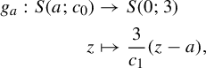 $$ \begin{align*} g_a: S(a;c_0) & \to S(0; 3)\\ z & \mapsto \frac{3}{c_1}(z-a), \end{align*} $$
for
 $a \in \mathbb {A}$
are all affine. Hence, if
 ${\underline {\theta }} \in (P^{\mathbb {N}}) ^- := \{(\ldots , a_{-n}, a_{-n+1},\ldots ,a_{-1},a_0): \, a_i \in P \;\text { for all } i \leq 0 \}$
has
 $\theta _0=a$
, then
 $k^{\underline {\theta }}$
is an affine transformation with derivative
 ${\textrm {Id}} \equiv 1 \in \mathbb {C}$
that carries a base point to
 $0$
. So, choosing for any of the pieces
 $S(a;c_0)$
the base point
 $c_a=a$
, we have
 $k^{\underline {\theta }}(z)=z-a$
, whose image is always the set
 $S(0;c_0)$
.
It is also easy to verify that, under our notation, for any
 $a, \, b \in P$
,
 $ f_{(a,b)}(z)=({c_1}/{3})z + a $
. We can then verify that the action of the renormalization operator is described by
 $$ \begin{align*} F^{\underline{\theta}(a,b)}(z)= \frac{c_1}{3}(z+b). \end{align*} $$
As already discussed, we denote every configuration pair
 $[h,h'] \in \mathcal {Q}$
by its representative that is scaled in the first coordinate
 $(A_h \circ h, A_h \circ h')$
. Similarly, any configuration pair
 $[(A,{\underline {\theta }}),(A',{\underline {\theta '}})] \in \mathcal {C} $
will be represented by the triple
 $(\underline {\theta },\underline {\theta }',A^{-1}\circ A')$
, as pointed out in the paragraph after Definition 3.4. However, proceeding by algebraically calculating the renormalization operator under this identification makes it hard to construct a recurrent compact set, so we also choose a geometric interpretation. For this, we may identify any map
 $B \in \textrm{Aff}(\mathbb {C})$
with
 $B(S(0;c_0))$
, which is a square embedded on
 $\mathbb {C}$
, considering the orientation of its vertices. Figure 2 exemplifies this idea for our identification.
The first square represents the configuration obtained from
 ${\textrm {Id}}$
. The second represents that from
 $A^{-1}\circ A' (z)=\alpha \cdot z+\beta $
. We will measure the distance of the configuration to the identity by the marked area the squares above have in common.
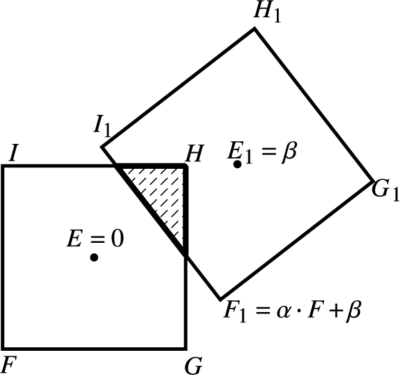
The square
 $FGHI$
represents
 ${\textrm {Id}}(S(0;c_0))$
with
 $E=0$
as its center. The square
 $F_1G_1H_1I_1$
represents the image of
 $S(0;c_0)$
by
 $A^{-1}\circ A'$
. If
 ${A}^{-1}\circ A'=\alpha \cdot z+ \beta , \, \alpha ,\,\beta \in \mathbb {C}$
, then the vector
 $\vec {EE_1}$
represents
 $\beta $
and
 $\alpha =({ F_1-\beta })/{F}$
, when
 $F,\,F_1,\,\beta $
are seen as complex numbers. In Figure 2, one can easily see that
 $\alpha =R\cdot \exp {\mathrm {i} \phi }$
, with
 $R>1$
and
 $\phi \in (0,\pi /4)$
, as the square was rotated no more than this angle.
For each
 $\kappa \in (0,1]$
and each complex number
 $\alpha $
, define
 $X^\kappa _\alpha $
as the set of all
 $B \in \textrm{Aff}(\mathbb {C})$
that are equal to
 $\alpha \cdot z + \beta , \text { for some } \beta \in \mathbb {C}$
, such that the area of
 $ S(0;c_0) \cap B(S(0;c_0) ) $
is at least
 $ \kappa \cdot c_0^2 \cdot (1+|\alpha |^2)$
, meaning that their intersection has an area of at least a small percentage of the sum of their areas. For
 $\kappa =0$
, we write
 $X^\kappa _\alpha $
for the set of all
 $B \in \textrm{Aff}(\mathbb {C}) \text { that are equal to } \alpha \cdot z + \beta , \text { for some } \beta \in \mathbb {C}$
, such that
 $ S(0;c_0) \cap B(S(0;c_0) ) \neq \emptyset $
. For example, if we consider the affine map identified in Figure 2, it is true that for
 $\kappa $
very close to
 $0$
, it is in
 $ X^\kappa _\alpha $
. Also for any real number
 $c \in (0,1]$
, define the set
 $R_{c}=\{z \in \mathbb {C};\, {c}^{1/2} \leq |z| \leq {c}^{-1/2}\}$
.
The recurrent compact set
 $\mathcal {L}$
we will construct on the subsequent lines will not depend on the limit geometries, that is,
 $\mathcal {L} = \Sigma ^- \times {\Sigma '}^{-} \times L = (P^{\mathbb {N}})^- \times (P^{\mathbb {N}})^- \times L $
, where L is a subset of
 $\textrm{Aff}(\mathbb {C})$
. Additionally, it is composed by three parts. The first one, which we call ‘central’ and denote by
 $\mathcal {L}_0$
, is made up of affine transformations
 $B = \alpha \cdot z + \beta \in \textrm{Aff}(\mathbb {C})$
such that
 $\alpha \in R_{c_1/3} $
, or in other words,
 $\ln {|\alpha|}$
belongs to an interval around
 $0$
; and
 $\beta $
is such that
 $B \in X_{\alpha }^{\kappa _1}$
for some value of
 $\kappa _1$
very close to
 $0$
to be chosen later.
In addition to this central part, two ‘lateral’ parts are in
 $\mathcal {L}$
, which we denote by
 $\mathcal {L}_1$
and
 $\mathcal {L}_{-1}$
. To construct them, we will chose a real number
 $c_2$
between
 $\tfrac 14$
and
 $ {c_1}/{3}$
, assuming
 $c_1$
is sufficiently close to
 $1$
. The first one,
 $\mathcal {L}_1$
, is made up by the affine transformations
 $B = \alpha \cdot z + \beta \in \textrm{Aff}(\mathbb {C})$
such that
 $\alpha \in R_{c_2}$
and
 $|\alpha |> (3/c_1)^{1/2}$
, in other words,
 $\ln {\lvert \alpha \rvert }$
belongs to an interval to the right of
 $0$
and sharing its left border with the central one; and
 $\beta $
is such that
 $B \in X^{\kappa _2}_\alpha $
, where
 $\kappa _2$
is some small constant larger than
 $\kappa _1$
to be chosen later. The other one,
 $\mathcal {L}_{-1}$
, is defined in a symmetrical manner, being made up by the affine transformations
 $B = \alpha \cdot z + \beta \in \textrm{Aff}(\mathbb {C})$
such that
 $\alpha \in R_{c_2}$
and
 $|\alpha | < (c_1/3)^{1/2}$
; and
 $\beta $
is such that
 $B \in X^{\kappa _2}_\alpha $
for the same value of
 $\kappa _2$
already stated.
For each
 $v = (\underline {\theta },\underline {\theta }',B) \in \mathcal {L}$
, we will find a renormalization that carries it to the interior of
 $\mathcal {L}$
. If it belongs to the central part
 $\mathcal {L}_0$
, we can find a renormalization
 $\mathcal {T}_{\underline {a},\underline {a}'}$
, where
 $\underline {a}$
and
 $\underline {a}'$
have size one, which carries v to a point in
 $\mathcal {L}_0$
preserving the coefficient
 $\alpha $
of B. This may not be enough to take
 $v \in \textrm{int}\,\mathcal {L}_0$
. However, if
 $\kappa $
, the largest value such that
 $B \in X^\kappa _\alpha $
, is smaller than
 $\kappa _2$
, we will prove that v is carried to
 $(\underline {\theta }\underline {a},\underline {\theta }\underline {a}',B')$
, where
 $B' \in X_{\alpha }^{\lambda \kappa }$
for some
 $\lambda> 1$
. After successive iterations of these renormalizations, v will be carried to the interior of
 $\mathcal {L}_0$
. If v belongs to any of the lateral parts, then we will find a renormalization
 $\mathcal {T}_{\underline {a},\underline {a}'}$
, where
 $\underline {a}$
and
 $\underline {a}'$
have combined size equal to one, which carries it to the central part, to its portion that is close to the other lateral part. See Figure 3 for an illustration.
A diagram representing the recurrent compact set. The coordinate
 $\beta $
is measured by
 $\kappa (\beta )$
, the proportion of area of intersection between the original square and its image by
 $\alpha \cdot z + \beta $
. This way, being closer to the axis means that this area is close to the maximal proportion, whereas being far means it is close to zero. The arrows indicate the action of the renormalizations considered above. Note that
 $[{\textrm {Id}}, {\textrm {Id}}]$
is represented by the origin.
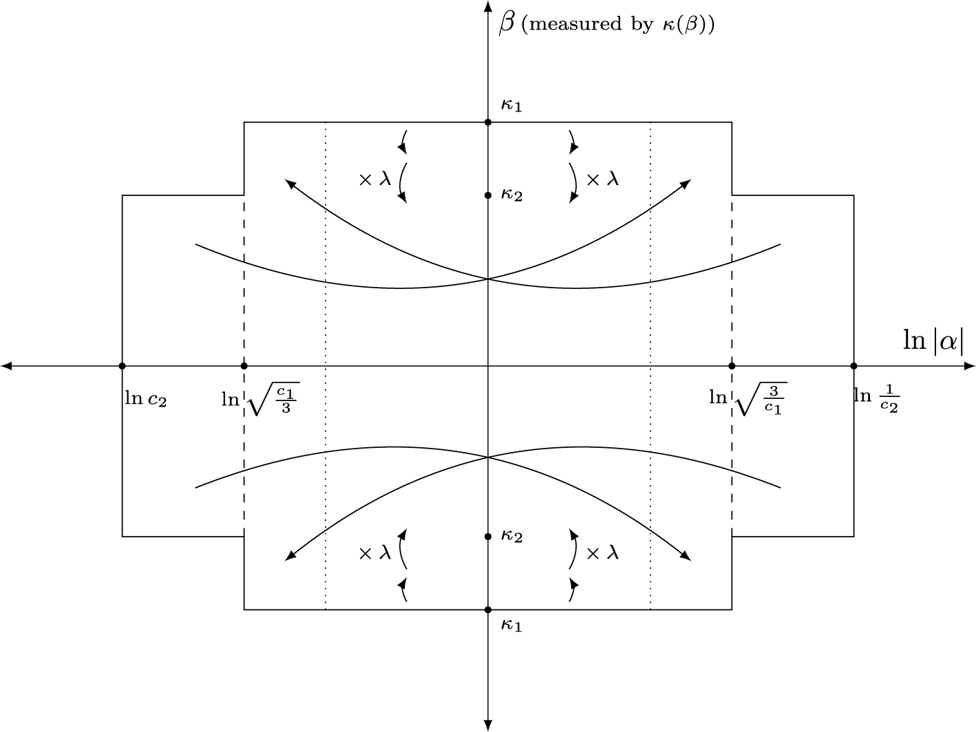
Having in mind the plan just described, let
 $\tfrac 14< ({c_1}/{3}) = c_3 < \tfrac 13$
and
 $\kappa _0 = {c_3}/({36(1 + c_3)})$
. The first step is the following claim.
Claim 4.2. If
 $\kappa < \kappa _0$
then, for any
 $B \in X^0_\alpha \setminus X^{\kappa }_\alpha $
with
 $\alpha \in R_{c_3}$
, the intersection
 $S(0;c_0) \cap B(S(0;c_0))$
is contained in one of the four strips
 $S_1=\{z;\,{\mathrm{Re}}(z)> ({c_0}/{3})\} \cap S(0;c_0)$
,
 $S_2=\{z;\,{\mathrm{Re}}(z) < -({c_0}/{3})\} \cap S(0;c_0)$
,
 $S_3=\{z;\,{\mathrm{Im}}(z)> ({c_0}/{3})\} \cap S(0;c_0)$
, or
 $S_4=\{z;\,{\mathrm{Im}}(z) < -({c_0}/{3})\} \cap S(0;c_0)$
. It is also contained in one of the four strips
 $B(S_i)$
for
 $i=1,2,3,4$
.
Proof. Let
 $S_m$
denote the smallest square among
 $S(0;c_0)$
and
 $B(S(0;c_0))$
, and
 $S_M$
the other one. Let
 $l_m$
and
 $l_M$
be the length of their sides, respectively, and
 $|S_m|$
and
 $|S_M|$
their areas. Further, let
 $\tfrac 23S_m$
denote the square with the same center as
 $S_m$
but side equal to
 $\tfrac 23$
of the original. Define
 $\tfrac 23S_M$
in the analogous way. If the conclusion fails, then
 $S_m$
intersects
 $\tfrac 23S_M$
or
 $S_M$
intersects
 $\tfrac 23S_m$
. Indeed, if
 $S_m$
does not intersect
 $\tfrac 23S_M$
, then there is a line separating these squares. The half-plane defined by it that contains
 $S_m$
intersects
 $S_M$
in a region contained in at most one strip of
 $S_M$
. The best way to see this is to translate the line until one of the vertices of
 $\tfrac 23S_M$
belongs to it. The analysis of the other case is analogous. See Figure 4 for an illustration.
The line separating the squares
 $S_m$
and
 $\tfrac 23S_M$
. The outer square on the right-hand side denotes the square
 $S_M$
. Notice that the intersection between the line separating the plane and the square
 $S_M$
is contained inside one strip.
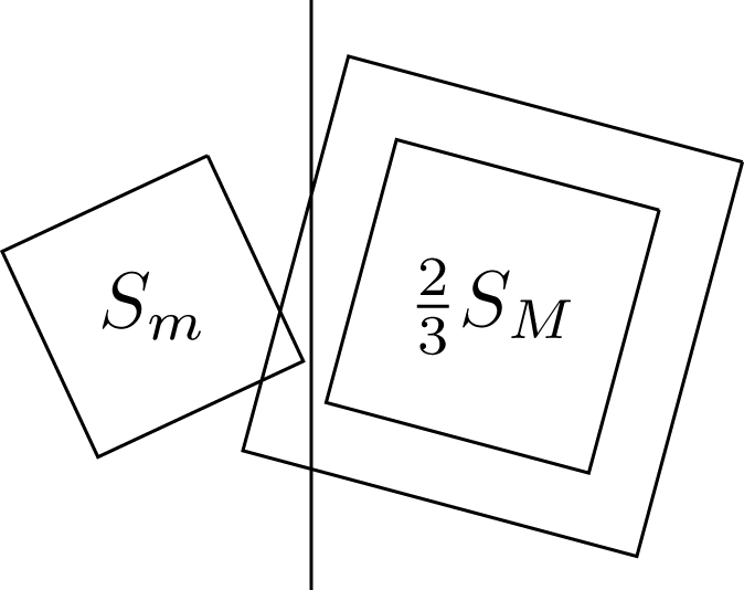
Now, suppose
 $S_m$
intersects
 $\tfrac 23S_M$
and let p be a point in this intersection. Consider a square centered at p congruent to
 $S_m$
whose sides are parallel to the sides of
 $S_m$
, that is, a translation of
 $S_m$
. Divide it into four smaller squares sharing a common vertex at p. One of them is contained in
 $S_m$
. If it is also contained in
 $S_M$
, then the area of their intersection is at least
 $\tfrac 14|S_m|$
. See Figure 5 for an illustration.
The central square divided into four smaller squares represents the square centered at p used in the proof of Claim 4.2. The point p belongs to
 $\tfrac 23S_M$
, which was not drawn to avoid confusion. The highlighted smaller square belongs to
 $S_m$
.
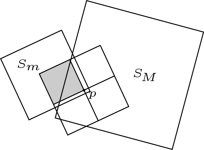
Suppose it is not. The diagonal of this smaller square defines an isosceles triangle with a right angle at p, the cathetuses having length equal to
 $\tfrac 12l_m$
. If they are both contained in
 $S_M$
, then the area of intersection between
 $S_m$
and
 $S_M$
is at least
 $\tfrac 18$
of that of
 $S_m$
, as this triangle would be contained in both. If just one of the cathetuses is entirely contained in
 $S_M$
, the part of the other one (which intersects the border of
 $S_M$
) that is contained in
 $S_M$
is a segment of length at least
 $\tfrac 16l_M$
; therefore, the intersection area is at least
 $\tfrac 12\cdot \tfrac 12 \cdot \tfrac 16 = \tfrac {1}{24} $
of the area of
 $S_m$
.
Finally, if both cathetuses intersect the border of
 $S_M$
, they either intersect this border on the same side of
 $S_M$
or in a pair of adjacent ones. In the first case, the distance between the intersection points with the border is at least
 $\tfrac 13l_M$
. Considering the triangle with base determined by these two points and the other vertex being p, the area of intersection between
 $S_m$
and
 $S_M$
is at least
 $\tfrac 12\cdot \tfrac 13\cdot \tfrac 16\cdot |S_M|= \tfrac {1}{36}|S_M|$
, because the height of this triangle is at least
 $\tfrac 16l_M$
and it is contained in both
 $S_m$
and
 $S_M$
. In the other case, the worst case scenario happens when p coincides with a vertex of
 $\tfrac 23S_M$
, but in this case, a direct calculation shows that the area of intersection is equal to
 $\tfrac {1}{36}|S_M|$
. The argument in the case where
 $S_M$
intersects
 $\tfrac 23S_m$
is analogous, and we conclude in both cases that the area of
 $S_m \cap S_M$
is at least
 $\tfrac {1}{36}|S_m|$
. Because
 ${|S_m|}/({|S_m|+|S_M|}) \ge {c_3}/({1+c_3})$
, the claim follows.
We divide the construction of
 $\mathcal {L}$
into parts. In each of them, we find constraints for
 $c_1$
in terms of
 $\kappa _1$
,
 $\kappa _2$
, and
 $c_2$
. In the end, if
 $\kappa _2$
,
 $\kappa _1$
, and
 $c_2$
are appropriately chosen, then there is some
 $c_1$
such that the resultant compact set is indeed recurrent.
Part 1 (Central part of
 $\mathcal {L}$
and
 $B \in X^{\kappa }_{\alpha }$
for small values of
 $\kappa $
). Let
 $\alpha \in R_{{c_1}/{3}}$
and
 $0<\kappa <\kappa _0$
. First, we show that if
 $c_1$
is really close to
 $1$
, for any
 $v \in \mathcal {C}$
identified by
 $(\underline {\theta },\underline {\theta }',B)$
with
 $B \in X^\kappa _\alpha \setminus X^{\kappa _0}_\alpha $
, we can find a pair of letters
 $(a,a') \in P^2$
such that the renormalization
 $ \mathcal {T}_{{\theta }_0a,{\theta }^{\prime }_0a'}$
carries v to
 $(\underline {\theta }a,\underline {\theta }'a',B')$
with
 $B' \in X^{\kappa '}_\alpha $
satisfying
 $1>\kappa ' > \kappa \cdot \lambda $
, where
 $\lambda> 1$
is a constant to be determined.
Any of these renormalization operators has a very simple visual description when we consider the graphical identification we defined in this section. Precisely, it carries the square that represents B to an inner square
 $Q_{B(a')}$
that is centered at the point
 $B(({c_1}/{3})a')$
and whose side length is equal to
 $|\alpha| ({c_1}/{3})c_0.$
The square that represents the identity is carried into
 $S(({c_1}/{3})a;({c_1}/{3})c_0)$
. It is necessary to rescale the pair by an affine transformation that carries the last one to
 $S(0;c_0)$
, but such action preserves the area proportion of the intersection.
We begin by observing that because
 $B \in X^0_\alpha \setminus X^{\kappa _0}_\alpha $
, we can assume, without loss of generality for our next calculation, that
 $S(0;c_0) \cap B(S(0;c_0)) \subset S_1 \cap B(S_1)$
. Dividing
 $S_1$
into three squares of side length
 ${c_0}/{3}$
,
 $Q_1,\,Q_2,\,Q_3$
, we observe that it is impossible for
 $(Q_i) \cap B(Q_j)$
to be non-empty for all pairs
 $(i,j),\,i,j =1,2,3$
.
Now, we remember that the area of the intersection between two subsets of
 $\mathbb {C}$
is at least the sum of their areas minus the area of their union. As a consequence, the area of
 $$ \begin{align*} \bigcup_{a \in P}S\bigg(\frac{c_1}{3}a; c_0\cdot \frac{c_1}{3}\bigg) \cap \bigcup_{a' \in P} B\bigg( S\bigg(\frac{c_1}{3}a';c_0 \cdot \frac{c_1}{3}\bigg)\bigg) \end{align*} $$
is at least
 $c_0^2$
multiplied by
 $c^2_1(1+|\alpha |^2) - (1-\kappa )(1+|\alpha |^2) $
, because
 $c_0^2 \cdot c^2_1(1+|\alpha |^2)$
is equal to the sum of the areas of the
 $18$
squares and their union is contained in
 $S(0;c_0) \cup B(S(0;c_0))$
, and hence has area at most
 $c_0^2 \cdot (1-\kappa )(1+|\alpha |^2)$
. This area is divided along at most eight intersections of the type
 $S((c_{1}/3)a; c_0\cdot {c_1}/{3}) \cap B( S(({c_1}/{3})a';c_0 \cdot {c_1}/{3})) \neq \emptyset $
for
 $(a,a') \in P^2$
. Because the areas of these squares are
 $c_0^2$
multiplied by
 $({c_1}/{3})^2$
and
 $({c_1}/{3})^2\cdot |\alpha |^2 $
, respectively, we need only to show that for
 $c_1$
big enough,
 $$ \begin{align*} (1+|\alpha|^2) \frac{(c_1^2 - (1-\kappa))}{8} \geq (1+|\alpha|^2) \frac{c_1^2 \cdot \lambda \cdot \kappa }{9}, \end{align*} $$
and it is clear that we can choose
 $c_1 < 1$
and
 $\lambda> 1$
both close to
 $1$
respecting all the previously fixed constraints in a way that the inequality above is true. Notice that as
 $c_1$
gets closer to
 $1$
, the distance
 $\delta $
between the pieces defining the Cantor set K has to be closer to
 $0$
. Moreover, if we fix
 $\kappa _1 < \kappa _0$
and choose
 $c_1$
such that
 $$ \begin{align} c_1^2> \frac{9-9\kappa_1}{9-8\kappa_1}, \end{align} $$
then there is some
 $\lambda> 1$
such that for any
 $\kappa _1 \le \kappa \le \kappa _0$
and any
 $v \equiv (\underline {\theta },\underline {\theta }',B)$
with
 $B \in X^\kappa _\alpha \setminus X^{\kappa _0}_\alpha $
, we can find a pair of letters
 $(a,a') \in P^2$
such that the renormalization
 $ \mathcal {T}_{{\theta }_0a,{\theta }^{\prime }_0a'}$
carries v to
 $(\underline {\theta }a,\underline {\theta }'a',B')$
with
 $B' \in X^{\lambda \kappa }_\alpha $
.
Part 2 (Central part of
 $\mathcal {L}$
and
 $B \in X^{\kappa }_{\alpha }$
for large values of
 $\kappa $
). However, if
 $B \in X^{\kappa _0}_\alpha $
with
 $\kappa \geq \kappa _0 $
,
 $\alpha \in R_{c_3 = {c_1}/{3}}$
, and
 $\xi \in (0,1)$
, the intersection
 $$ \begin{align*}\bigcup_{a \in P}S\bigg(\frac{c_1}{3}a; \xi \cdot c_0\cdot \frac{c_1}{3}\bigg) \cap \bigcup_{a' \in P} B\bigg( S\bigg(\frac{c_1}{3}a';\xi \cdot c_0 \cdot \frac{c_1}{3}\bigg)\bigg)\end{align*} $$
is empty only if
 $$ \begin{align*} c_1^2 \cdot \xi^2 \le \bigg(1-\frac{c_3}{36(1+c_3)}\bigg) = 1 - \kappa_0, \end{align*} $$
because the area of the union of the
 $18$
squares is equal to
 $c_1^2\xi ^2 \cdot ( 1+\lvert \alpha \rvert ^2)c_0^2$
and they are all contained in
 $S(0;c_0) \cup B(S(0;c_0))$
, whose area is at most
 $(1 - \kappa _0)( 1+\lvert \alpha \rvert ^2)c_0^2$
. Hence, if
 $\xi $
is sufficiently large, for some pair
 $(a,a') \in P^2$
,
 $$ \begin{align} S\bigg(\frac{c_1}{3}a;\xi \cdot \frac{c_1}{3} c_0\bigg) \cap B\bigg(S\bigg(\frac{c_1}{3}a'; \xi \cdot \frac{c_1}{3} c_0\bigg)\bigg) \neq \emptyset. \end{align} $$
Assume that
 $\xi> 1 - c_1/3\sqrt {2}$
.
Claim 4.3. For this said pair, the area of the intersection
 $$ \begin{align*} S\bigg(\frac{c_1}{3}a;\frac{c_1}{3} c_0\bigg) \cap B\bigg(S\bigg(\frac{c_1}{3}a'; \frac{c_1}{3} c_0\bigg)\bigg) \end{align*} $$
is larger than or equal to
 $({(1-\xi )^2}/{4}) ({c_1^2}/{9})(1+|\alpha |^2)c_0^2$
.
Proof. Let x be a point in the intersection in equation (4.2). The square centered at x whose sides are parallel to the sides of
 $S(0;1)$
and has lengths
 $(1-\xi )c_0c_1/3$
is contained inside
 $ S(({c_1}/{3})a; ({c_1}/{3}) c_0)$
. Denote it by
 $R_1$
. Analogously, the square centered at x whose sides are parallel to the sides of
 $B(S(0;1))$
and has lengths
 $(1-\xi ) \lvert \alpha \rvert c_0c_1/3 $
is contained inside
 $B(S(({c_1}/{3})a'; ({c_1}/{3}) c_0)))$
. Denote it by
 $R_2$
.
The intersection between
 $R_1$
and
 $R_2$
lies inside
 $$ \begin{align*} S\bigg(\frac{c_1}{3}a;\frac{c_1}{3} c_0\bigg) \cap B\bigg(S\bigg(\frac{c_1}{3}a'; \frac{c_1}{3} c_0\bigg)\bigg). \end{align*} $$
Suppose without loss of generality that
 $\lvert \alpha \rvert < 1$
. The argument in the other case is analogous. In this case,
 $R_2$
is smaller than
 $R_1$
. If
 $R_2$
is not contained inside
 $R_1$
, then the intersections of the diagonals of
 $R_2$
with the sides of
 $R_1$
determine a square whose area is greater than
 ${(1 - \xi )^2}/{2}\cdot ({c_1^2}/{9})c_0^2$
contained both in
 $R_1$
and
 $R_2$
. The estimate follows as
 $1 + \lvert \alpha \rvert ^2 \le 2 $
.
If
 $R_2$
is contained inside
 $R_1$
, we adapt the argument a little. Dividing
 $R_2$
into four congruent squares, we observe that at least one of them can be exchanged by one sharing the same vertex x but side lengths equal to
 $\lvert \alpha \rvert /2$
so that the resultant figure is still contained in
 $B(S((c_1/3)a'; (c_1/3)c_0)))$
. Because
 $(1 - \xi ) \sqrt {2} < c_1/3 $
, the intersection of this bigger square with
 $R_1$
is a right-angled sector centered at x and so has an area of exactly
 $1/4$
of the area of
 $R_1$
.
Therefore, the area of the intersection is at least
 $(({(1- \xi )^2}/{4})\cdot ({c_1^2}/{9})c_0^2 + (({3(1 - \xi )^2\lvert \alpha \rvert ^2})/{4})\cdot ({c_1^2}/{9})c_0^2)$
and the estimate follows.
Now,
 $ 1 - \kappa _0 = 1 - ({c_3}/{36(1+c_3)}) \le {179}/{180}$
, because
 $c_3 \ge \tfrac 14$
. Hence, if
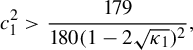 $$ \begin{align} c_1^2>\frac{179}{180 (1-2\sqrt{\kappa_1})^2 }, \end{align} $$
there is some value of
 $\xi ^2$
smaller than or equal to
 $(1-2\sqrt {\kappa _1})^2$
(and so
 $(1 - \xi )^2/4 \ge \kappa _1$
) such that
 $c_1^2 \xi ^2> 1 - \kappa _0$
, and hence
 $$ \begin{align*} \bigcup_{a \in P}S\bigg(\frac{c_1}{3}a; \xi \cdot c_0\cdot \frac{c_1}{3}\bigg) \cap \bigcup_{a' \in P} B\bigg( S\bigg(\frac{c_1}{3}a';\xi \cdot c_0 \cdot \frac{c_1}{3}\bigg)\bigg) \neq \emptyset. \end{align*} $$
That way, following Claim 4.3, given
 $v \in \mathcal {C}$
identified by
 $(\underline {\theta },\underline {\theta }',B)$
with
 $B \in X^{\kappa _0}_\alpha $
and
 $\alpha \in R_{{c_1}/{3}}$
, we can find a pair of letters
 $(a,a') \in P^2$
such that the renormalization
 $ \mathcal {T}_{{\theta }_0a,{\theta }^{\prime }_0a'}$
carries v to
 $(\underline {\theta }a,\underline {\theta }'a',B')$
with
 $B' \in X^{\kappa _1}_\alpha $
.
We are almost able to construct the recurrent compact set. Before that, fix
 $\tfrac 14 < c_2 < ({c_1}/{3})$
.
Part 3 (Lateral parts). Let
 $\kappa _2 < \kappa _0$
and
 $\alpha \in R_{c_2} \setminus R_{{c_1}/{3}}$
. We divide into the following cases.
(1)
 $|\alpha |^2> ({3}/{c_1})$
. In this case, if we consider any
 $v \equiv (\underline {\theta },\underline {\theta }', B) \in \mathcal {C}$
such that
 $B = \alpha \cdot z + \beta \in X^{\kappa _2}_\alpha $
then, by choosing
 $c_1$
sufficiently close to
 $1$
and
 $\kappa _1$
close to
 $0$
, we can find a renormalization operator
 $ \mathcal {T}_{\emptyset ,{\theta '}_0a'} $
that sends v to
 $(\underline {\theta }, \underline {\theta }'a',B' )$
with
 $B'=\alpha ' \cdot z + \beta ', \,\alpha ' \in R_{{c_1}/{3}},\,\beta ' \in \mathbb {C} $
and
 $B' \in X^{\kappa _1}_{\alpha '}$
. Checking the formula for the renormalization operator, we have that
 $\alpha ' = \alpha \cdot {c_1}/{3} \in R_{{c_1}/{3}}$
by definition, so the expansion part of
 $B'$
is guaranteed. Pay attention to the importance of the choice
 $ \mathcal {T}_{\emptyset ,{\theta '}_0a'} $
. The hard part is to control the translation part of
 $B'$
.
Now, we know that the area of
 $S(0;c_0)\cup B(S(0;c_0))$
is at most
 $c_0^2(1+|\alpha |^2)(1-\kappa _2)$
. This implies that the area of
 $$ \begin{align*} S(0;c_0) \cap \bigcup_{a \in P} B\bigg(S\bigg(\frac{c_1}{3}a;c_0 \cdot \frac{c_1}{3}\bigg)\bigg) \end{align*} $$
is at least
 $c_0^2(1+c_1^2|\alpha |^2 - (1+|\alpha |^2)(1-\kappa _2)) $
– it is the same argument as before, but this time we only have ten squares (
 $S(0;c_0)$
and
 $B(S(({c_1}/{3})a;c_0 \cdot {c_1}/{3}))$
for
 $a \in P$
) whose areas add up to
 $c_0^2(1+c_1^2|\alpha |^2)$
. By the pigeonhole principle, for some
 $a \in P$
, the area of
 $S(0;c_0) \cap B(S(({c_1}/{3})a;c_0 \cdot {c_1}/{3})$
is at least
 $\tfrac 19$
of this total area. Thus, if
 $c_1$
and
 $\kappa _1$
satisfy
 $$ \begin{align*} c_0^2\frac{(1+c_1^2|\alpha|^2 - (1+|\alpha|^2)(1-\kappa_2))}{9} \geq c_0^2\cdot \kappa_1 \bigg(1+\bigg(\frac{c_1}{3}\bigg)^2|\alpha|^2\bigg), \end{align*} $$
then, for some
 $a \in P$
, the area of intersection between
 $S(0;c_0)$
and
 $B(S(({c_1}/{3})a;c_0 \cdot {c_1}/{3})$
is at least
 $\kappa _1$
times the sum of their areas. However, this inequality is equivalent to
 $$ \begin{align*} c_1^2 \cdot (1 - \kappa_1) \ge 1+ \frac{9 \kappa_1}{|\alpha|^2} - \frac{1 + | \alpha |^2}{| \alpha |^2} \kappa_2. \end{align*} $$
Hence, if
 $c_1^2 \geq 1+ 4 \kappa _1 - ({5 \kappa _2}/{4})$
,
 $$ \begin{align*} c_1^2 \cdot (1 - \kappa_1) \ge c_1^2 - \kappa_1 \ge 1 + 3 \kappa_1 - \frac{5 \kappa_2}{4} \ge 1+ \frac{9 \kappa_1}{|\alpha|^2} - \frac{1 + | \alpha |^2}{| \alpha |^2} \kappa_2, \end{align*} $$
because
 $| \alpha |^2$
belongs to the interval
 $(3, 4)$
. In other words, if
 $\kappa _1$
is sufficiently small and
 $c_1$
close to
 $1$
, the condition
 $$ \begin{align} c_1^2 \geq 1+ 4 \kappa_1 - \frac{5 \kappa_2}{4} \end{align} $$
is satisfied and so there is a choice of
 $a' \in P$
such that
 $\mathcal {T}_{\emptyset ,\underline {\theta }^{\prime }_0a'}$
carries
 $v \equiv (\underline {\theta }, \underline {\theta }', B)$
to
 $(\underline {\theta }, \underline {\theta }'a', B')$
with
 $B'\in X^{\kappa _1}_{\alpha '}$
, which concludes this part.
(2)
 $|\alpha |^2 < ({c_1}/{3})$
. This case is very similar to the previous one; the difference is that for
 $v \equiv (\underline {\theta },\underline {\theta }', B) \in \mathcal {C} $
such that
 $B=\alpha \cdot z+\beta \in X^{\kappa _2}_\alpha $
, we find a renormalization operator
 $\mathcal {T}_{{\theta }_0a,\emptyset }$
,
 $a \in P$
, that sends v to
 $(\underline {\theta }a, \underline {\theta }',B')$
with
 $B'=\alpha ' \cdot z + \beta ', \,\alpha ' \in R_{{c_1}/{3}},\,\beta ' \in \mathbb {C}$
and
 $B'\in X^{\kappa _1}_{\alpha '}$
. Once again,
 $\alpha '=\alpha \cdot ({3}/{c_1}) \in R_{{c_1}/{3}}$
, so we proceed to check the translation part.
Again, the area of
 $S(0;c_0)\cup B(S(0;c_0))$
is at most
 $c_0^2(1+|\alpha |^2)(1-\kappa _2)$
. By definition,
 $B'=(F^{\underline {\theta }a})^{-1}\circ B$
, but because
 $F^{\underline {\theta }a}$
is affine,
 $B' \in X^{\kappa _1}_{\alpha '}$
if, and only if, the area of
 $$ \begin{align*} F^{\underline{\theta}a}(S(0;c_0) ) \cap B(S(0;c_0)) = S\bigg(\frac{c_1}{3}a;\ c_0\cdot \frac{c_1}{3}\bigg) \cap B(S(0;c_0)) \end{align*} $$
is larger than
 ${c_0^2 \cdot \kappa _1 (({c_1}/{3})^2+|\alpha |^2)}$
.
Arguing as in the previous item, the area of
 $$ \begin{align*} \bigcup_{a \in P} S\bigg( \frac{c_1}{3}a;c_0 \cdot \frac{c_1}{3} \bigg) \cap B(S(0;c_0)) \end{align*} $$
is at least
 $c_0^2 \cdot (c_1^2 + |\alpha |^2 - (1+|\alpha |^2)(1-\kappa _2))$
and it is divided among the nine squares
 $S( ({c_1}/{3})a;c_0 \cdot {c_1}/{3} )$
. By the pigeonhole principle, if
 $$ \begin{align*} \frac{c_1^2 + |\alpha|^2 - (1+|\alpha|^2)(1-\kappa_2)}{9} \geq \kappa_1 \bigg(\bigg(\frac{c_1}{3}\bigg)^2 + |\alpha|^2\bigg), \end{align*} $$
then, for some
 $a \in P$
, the area of intersection between
 $S( ({c_1}/{3})a;c_0 \cdot {c_1}/{3} )$
and
 $B(S(0;c_0))$
is at least
 $\kappa _1$
times the sum of their areas. Thus, there is a renormalization operator
 $\mathcal {T}_{ \theta _0a,\emptyset }$
that sends v to
 $(\underline {\theta } a, \underline {\theta }', B')$
with
 $B' \in X^{\kappa _1}_{\alpha '}$
and
 $\alpha ' \in R_{{c_1}/{3}}$
.
However, this inequality is equivalent to
 $$ \begin{align*} c_1^2\cdot(1-\kappa_1) \ge 1 + 9 \kappa_1| \alpha| ^2 - (| \alpha |^2+1)\kappa_2, \end{align*} $$
which is satisfied when
 $c_1^2 \ge 1 + 4\kappa _1 - ({5 \kappa _2}/{4})$
(equation (4.4)), because then
 $$ \begin{align*} c_1^2 \cdot (1 - \kappa_1) \ge c_1^2 - \kappa_1 \ge 1 + 3 \kappa_1 - \frac{5 \kappa_2}{4} \ge 1+ 9 \kappa_1 |\alpha|^2 - (1 + | \alpha |^2 ) \kappa_2, \end{align*} $$
because
 $| \alpha |^2$
belongs to the interval
 $(\tfrac 14, \tfrac 13)$
.
It is no surprise that the quota would be the same given the symmetry of the problem.
Thus, we can construct a recurrent compact set
 $\mathcal {L} \subset \mathcal {C}$
as a union
 $\mathcal {L} = \mathcal {L}^{-1} \cup \mathcal {L}^{0} \cup \mathcal {L}^{1}$
, where
 $\mathcal {L}^i = (P^{\mathbb {N}})^- \times (P^{\mathbb {N}})^- \times L^i$
for
 $i=-1,\,0,\,1$
, and the
 $L^i$
are defined as:
-
•
${{L}^1 = \bigcup _{\alpha \in R_{c_2}^1} X^{\kappa _2}_{\alpha }} $
;
${R_{c_2}^1 = \{ \alpha \in \mathbb {C}, \, \sqrt {{3}/{c_1}} < |\alpha | \le \sqrt {{1}/{c_2}} \} }$
; -
•
${{L}^{-1} = \bigcup _{\alpha \in R_{c_2}^{-1} } X^{\kappa _2}_\alpha }$
;
${ R_{c_2}^{-1} = \{\alpha \in \mathbb {C}, \, \sqrt {c_2} \le |\alpha | < \sqrt {{c_1}/{3}}\}} $
; -
•
${{L}^0 = \bigcup _{\alpha \in R_{{c_1}/{3}}} X^{\kappa _1}_\alpha }$
;


and
 $\kappa _1,\, \kappa _2, c_1$
, and
 $c_2$
are chosen respecting the constraints we have already fixed. This means that
 $\kappa _1$
is sufficiently small and
 $c_1$
is sufficiently close to
 $1$
so as to make equations (4.1), (4.3), and (4.4) true. As we have already shown, for almost all
 $v \in \mathcal {L}$
, one of the renormalization operators
 $\mathcal {T}$
we already found above makes
 $\mathcal {T}(v) \in \text {int}(\mathcal {L})$
. We need only to show that for
 $v=(\underline {\theta },\underline {\theta '}, B)$
, where
 $B = \alpha \cdot z + \beta $
with
 $|\alpha |^2= {c_1}/{3}$
or
 ${3}/{c_1}$
and
 $B \in X^{\kappa _1}_\alpha \setminus X^{\kappa _2}_\alpha $
, we can find a renormalization that carries it to the interior of
 $\mathcal {L}$
. Yet, in this case, we can repetitively apply the renormalization operators previously described appropriate to this case to obtain a sequence
 $v_n = \mathcal {T}_{\underline {\theta }^na_n,{\underline {\theta }'}^na^{\prime }_n} (v_{n-1})$
for which:
-
•
$v_0=v$
; -
•
$({\underline {\theta }^n,{\underline {\theta }'}^n}) = ({\underline {\theta }^{n-1}a_{n-1},{\underline {\theta }'}^{n-1}{a'}_{n-1}})$
; and -
•
$v_n\in X^{\lambda ^n\kappa _1}_\alpha $
.


Hence, if n is large enough,
 ${\lambda ^n\kappa _1}> \kappa _2 $
, which implies that
 $v_n \in \text {int}(\mathcal {L})$
as we wished to obtain.
Remark 4.4. Given the constraints on the proof above, more importantly,
 $\kappa _2 < ({c_3}/{36(1+c_3)}) $
, we can calculate that for
 $$ \begin{align*}c_1^2 \geq {\min_{\kappa_1 \in [0,1]} \max\bigg\{\frac{9-9\kappa_1}{9-8\kappa_1}, 1+4 \kappa_1-\frac{1}{144}, \frac{179}{180 (1-2\sqrt{\kappa_1})^2 }\bigg\}}, \end{align*} $$
 $\kappa _1$
can be chosen such that the construction above works at all steps. Some computation proves that
 $\delta \approx 5\cdot 10^{-8} $
is sufficiently small to the conclusion of Theorem 4.1. This quota is not optimal and may be greatly improved by adaptations in the argument, because a lot of area is ‘wasted’ in the estimates.
Acknowledgements
We would like to thank the anonymous referee for their very useful comments and suggestions. The paper was written while the first author was at IMPA and we thank them for their support and hospitality. This work was supported by CNPq and CAPES.
A Appendix
We need an adaptation of the
 $C^{r} $
section theorem, which can be found in the book by Shub [Reference Shub19, Theorem 5.18], to the case in which the base is not overflowing. Because we did not find a precise version of what we mean by this in the literature, we state the following version below and give a short argument on how a proof would work. We recommend reading the proof in Shub’s book beforehand.
Theorem A.1 (Adapted
$C^r$
section theorem)

Let
 $\Pi : E \to M$
be a
 $C^m$
vector bundle over a manifold M, with an admissible metric on E, and D be the disc bundle in E of radius C,
 $C>0$
a finite constant.
Let
 $h:U \subset M \to M$
be an embedding map of class
 $C^m$
(with a
 $C^m$
inverse too), U a bounded open set such that
 $ U \not \subset h(U) $
but
 $h(U) \cap U \neq \emptyset $
, and
 $F: E|_U \to E|_{h(U)}$
a
 $C^m$
map that covers h, that is,
 $\Pi \circ F = f \circ \Pi $
.
Let also
 $N \subset U$
be an open neighborhood of
 $ U\setminus h(U)$
and
 $s_0 : N \to D |_N$
a
 $C^r$
invariant section
 $(\lceil r \rceil \leq m, \; r\in \mathbb {R}, \; m \in \mathbb {N} )$
. By invariant we mean that whenever
 $x \in N$
and
 $h(x) \in N$
, we have
 $s_0(h(x)) = F( s_0(x) )$
. We also need the technical hypothesis that
 $N \subset U\setminus h^2(U)$
and
 $\overline {U\setminus N} \cap \overline {U \setminus h(U)} = \emptyset $
.
In this context, suppose that there is a constant k,
 $0 \leq k < 1$
, such that the restriction of
 $F $
to each fiber over
 $x \in U$
,
 $F_x : D_x \to D_{h(x)}$
is Lipschitz of constant at most k; that
 $h^{-1}$
is Lipschitz with constant
 $\mu $
; that
 $F^{(j)}$
,
 $s_0^{(j)}$
, and
 $ h^{(j)}$
are bounded for
 $0 \leq j < \lceil k \rceil $
,
 $j \in \mathbb {Z}$
; and
 $k \mu ^{r} <1$
. Then there is a unique invariant section
 $s: U \to D |_U$
(meaning that for
 $x \in U$
and
 $h(x) \in U$
, we have
 $s(h(x)) = F( s(x) )$
) with
 $s|_N = s_0$
and such a section is
 $ C^{r}$
.
Proof. The loss of the overflowing condition on h and U is overcome by the presence of the invariant section
 $s_0$
. The natural graph transform would carry sections over U to sections over
 $h(U)$
, but, because
 $s_0$
is invariant in
 $N \supset U\setminus h(U)$
, given any section s that agrees with
 $s_0$
in N, we are able to extend its graph transform from
 $h(U) \cap U$
back to the whole open set U. This idea comes from Robinson [Reference Robinson18]. In addition to this, very little has to be changed from the proof of Shub. The admissible hypothesis on the metric works the same way to allow us to work in the context of
 $E=M \times A$
, where A is a Banach space and E is equipped with the product metric d, and write a section as
 $s(x)=(x,\sigma (x))$
.
Next we consider the complete metric space
 $\Gamma ( U, D |_U; s_0 )$
of continuous sections over U bounded by C that agree with
 $ s_0$
on
 $N' \subset U$
, an open set such that
 $N\supset \overline {N'} \cap U \supset N' \supset U\setminus h(U)$
. Careful choice of
 $ N' $
allows us to use a
 $C^{\infty }$
function
 $\lambda $
on U that is equal to one on
 $N'$
and zero outside of N, and thus, taking
 $s=\lambda \cdot s_0$
yields a well-defined section that belongs to
 $\Gamma ( U, D |_U; s_0 )$
; which shows that it is not empty. Then consider
 $\Gamma _F: \Gamma ( U, D |_U; s_0 ) \to \Gamma ( U, D |_U; s_0 ) $
defined by
 $$ \begin{align*} \Gamma_F(s)(x)= \begin{cases} s(x)&\text{ if } x \in N' ,\\ F\circ s \circ h^{-1}(x) &\text{ if } x \in h(U). \end{cases} \end{align*} $$
Because s is equal to
 $s_0$
over
 $N'$
, it is invariant in this open set and the definition above is coherent. Also, because
 $k<1$
, this transformation is a contraction, so there is a unique section in
 $\Gamma ( U, D |_U; s_0 )$
fixed by
 $\Gamma _F$
. From now on, we denote it by s to simplify notation. If
 $x\in U$
and
 $h(x)\in U$
, this implies that
 $$ \begin{align*}s(h(x))=\Gamma_F(s)(h(x))=F\circ s \circ h^{-1}(h(x))=F(s(x)),\end{align*} $$
and hence s is an invariant section over U that agrees with
 $s_0$
on N.
The verification of regularity of s has some minor technical differences. First, we need to verify that if
 $0 \leq r < 1 $
, then s is r-Hölder in all U, that is, there is a constant
 $H>0$
such that
 $d((\sigma (x),\sigma (y)) \le H d(x,y)^r$
for all pairs
 $x,\, y \in U$
. To do so, we need some intermediate steps, which consider different locations of the points x and y.
Because s agrees with
 $s_0$
on N, it is r-Hölder on this set, so there is a constant
 $H'>0$
such that
 $d(\sigma (x),\sigma (y)) \leq H' d(x,y)^r$
for all
 $x, y \in N$
. Now,
 $U\setminus h(U)$
and
 $U \setminus N$
have a positive distance
 $\varepsilon $
between each other and the section s is bounded by C. So, if
 $x \in U\setminus h(U) $
and
 $y\in U\setminus N$
, we have
 $d(\sigma (x),\sigma (y)) \leq 2C \leq H' \varepsilon ^r \leq H' d(x,y)^r$
up to increasing the constant
 $H'$
. This allows us to write
 $d(\sigma (x),\sigma (y)) \leq H' d(x,y)^r$
for any pair
 $x \in U\setminus h(U)$
and
 $y \in U$
.
The map F is
 $C^m$
with
 $m \ge 1$
and so also r-Hölder. Hence there is a constant
 $\tilde {H}>0$
such that
 $d(F(e_1),F(e_2)) \le \tilde {H} d(e_1, e_2)^r \;\text { for all } e_1, e_2 \in E $
. As in the book, whenever
 $h^{-j}(x) \in U$
and
 $ h^{-j}(y) \in U$
for all
 $ j=0,\; 1, \; 2, \ldots , \; m $
, we have
 $$ \begin{align*} d(\sigma(x),\sigma(y)) \leq k^m d(\sigma (h^{-m}(x)), \sigma (h^{-m}(y))) + \tilde{H} \sum_{j=1}^{m} (\mu^{r})^j k^{j-1}(d(x,y))^{r}. \end{align*} $$
We are going to consider two cases.
If
 $x,y \in U$
are such that
 $h^{-j}(x) \in U$
and
 $h^{-j}(y) \in U$
for all
 $ j \in \mathbb {N} $
, we let
 $m \rightarrow \infty $
in the inequality above, and, because
 $k \mu ^{r} <1$
and
 $\sigma $
is bounded by C, the right-hand side converges to
 $\tilde {H} \cdot \tilde {C} d(x,y)^r$
, where
 $\tilde {C}={\mu ^r}/({1-k\mu ^r})$
.
If else, there is a finite maximal m such that
 $h^{-j}(x)$
and
 $ h^{-j}(y)$
belong to
 $ U$
for all
 $ j=0,\, 1,\, 2,\, \ldots ,\, m $
. In this case, we can assume without loss of generality that
 $h^{-m}(x) \in U \setminus h(U)$
. However then, using again the estimate above,
 $$ \begin{align*}& d(\sigma (x), \sigma(y)) \leq k^m d(\sigma (h^{-m}(x)), \sigma (h^{-m}(y))) + \tilde{H} \sum_{j=1}^{m} (\mu^{r})^j k^{j-1}(d(x,y))^{r} \\ &\quad\!\!{\leq}\kern1.5pt k^m\cdot H'\cdot d(h^{-m}(x),h^{-m}(y))^r\kern1pt{+}\kern1pt\tilde{H} \kern1pt{\cdot}\kern1pt \tilde{C} d(x,\kern-0.1pt y)^r \kern1.2pt{\leq}\kern1.2pt H' \kern1pt{\cdot}\kern1pt k^m \cdot \mu ^{mr} d(x,\kern-0.1pt y)^r \kern1pt{+}\kern1pt \tilde{H} \kern1pt{\cdot}\kern1pt \tilde{C} d(x,\kern-0.1pt y)^r\!, \end{align*} $$
because
 $h^{-m}(x) \in U\setminus h(U)$
and
 $h^{-m}(y) \in U$
. Again, because
 $k\mu ^r < 1$
, it follows that
 $d(\sigma (x),\sigma (y)) \leq (H'+\tilde {H} \cdot \tilde {C}) \cdot d(x,y)^r $
for any
 $x,y \in U$
. So this part is done after taking
 $H=H'+\tilde {H} \cdot \tilde {C}$
.
The smoothness is proved with the same argument as in the book adapted in some way as above. Using the same induction idea, in our case on
 $\lfloor k \rfloor $
, one can do as follows.
Let
 $\bar {E}$
be the fiber bundle over M with each fiber being equal to
 $L(T_xM, A)$
. As in Shub’s proof, the derivative of s, which we denote by
 $\partial s$
, can be seen as living in
 $\bar {E}$
if we ignore the trivial part and consider
 $\partial {s}(x)=(x,D\sigma (x))$
. The same construction from the book allows us to consider this bundle to be a trivial bundle with a product metric d equal to, when restricted to each fiber, the one obtained from the operator norm. Fix
 $\tilde {C}$
larger than
 $\Vert \partial {s}\Vert $
and let
 $\tilde {D}$
be the disc bundle of radius
 $\tilde {C}$
on
 $\bar {E}$
. Then the metric space
 $\Gamma (U,\tilde {D} |_U; \partial s_0)$
of continuous sections of
 $\tilde {D}$
that agree with
 $\partial s_0$
on
 $N'$
is complete. The graph transform
 $\gamma _{DF}(\tau )$
of a section
 $\tau (x) =(x,\varsigma (x))$
, where
 $\varsigma (x) \in L(T_xM , A)$
, is defined by
 $$ \begin{align*} \gamma_{DF}(\tau)(x)= \begin{cases} \partial s(x) &\text{ if } x \in N',\\ (x,\Gamma_{DF} (\varsigma(h^{-1}(x))) &\text{ if } x \in h(U) , \end{cases} \end{align*} $$
where
 $\Gamma _{DF}(L):= (\Pi _2 DF_{(x,\sigma (x))})\circ ({\textrm {Id}},L) \circ Dh^{-1}_{h(x)} $
for any linear transformation in
 $L \in (T_xM, A)$
and the compositions are just compositions of linear maps. This means that
 $$ \begin{align*} \Gamma_{DF}(L) = \Pi_2 D_1F_{(x,\sigma(x))}( Dh^{-1}_{h(x)}) + \Pi_2 D_2F_{(x,\sigma(x))} L ( Dh^{-1}_{h(x)}). \end{align*} $$
It is a fiber contraction of constant
 $k\mu <1$
.
To show that the invariant section
 $\tilde {\tau }$
indeed corresponds to the tangent to
 $s(x)=(x,\sigma (x))$
for all
 $ x \in U$
, we have to divide in cases as above.
If
 $x \in \bigcup _{n \in \mathbb {N}} h^n(N')$
, then it is true by definition of
 $ \partial s$
and the fact that
 $\tilde {\tau } $
is invariant and equal to
 $\partial s_0$
on
 $N'$
(remember that
 $s_0$
is
 $C^r$
).
If not, then for any
 $n \in \mathbb {N}$
, there is
 $\delta $
small enough such that if
 $d(x,y) < \delta $
, then
 $h^{-j}(x), h^{-j}(y) \in U$
for
 $j=0,1,2, \ldots , n$
. This comes from the fact that
 $x \in \bigcap _{i \in \mathbb {N}}h^i (U)$
and
 $h^n(U)$
is an open set around x. This is enough to show, by the same iteration argument, that
 $\text {Lip}_0(\sigma (x+y), \sigma (x) + \tilde {\varsigma }(x)(y))=0$
, which completes the proof.
Remark A.2. The condition
 $k\mu ^r<1$
may be replaced by a pointwise condition:
 $$ \begin{align*} k_x\cdot ({\textrm{Lip}}_{h(x)}(h^{-1}))^r < C < 1, \end{align*} $$
for every
 $x \in U$
, where
 $k_x$
is the Lipschitz constant of the fiber contraction
 $F_x$
,
 ${\textrm {Lip}}_{h(x)}(h^{-1})$
is the Lipschitz constant of
 $h^{-1}$
at the point
 $h(x)$
, and
 $C < 1$
is some constant uniform for all x. This is important for Remark 2.3. The proof is the same as above, changing k and
 $\mu $
for the corresponding
 $k_x$
and
 ${\textrm {Lip}}_{h(x)}(h^{-1})$
. To keep the clarity of the text, we chose to present only the simplified version.
Remark A.3. Observe that, from the argument above, if we just want to obtain an invariant section that is continuous, we can just make
 $m=r=0$
and consider just the case in which M is a topological space rather than a manifold.
Remark A.4. If we add the additional hypothesis that the maps
 $h \text {, } F \text {, } s_0$
, and all their derivatives are uniformly continuous, the proof above also shows that the invariant section varies continuously with the maps involved. More specifically, fixing
 $h, F, s_0$
and choosing any
 $h',F',s^{\prime }_0$
such that
 $h \text { and } h'$
are
 $C^m$
close and also their inverses;
 $F \text { and } F'$
are
 $C^m$
close (and
 $F'$
covers
 $h'$
);
 $s_0 \text { and } s^{\prime }_0$
are invariant (by
 $F \text { and } F' $
, respectively) and
 $C^r$
close; and
 $k \mu ^r < 1$
, then s and
 $s'$
are both close in the
 $C^ {r}$
topology. The proof is essentially the same as above and the details are left to the reader.
We now proceed to the proof of Theorem 2.2.
Proof of Theorem 2.2. The work of Pixton (Theorem 3.4 of [Reference Pixton17]) shows that we can construct a not necessarily smooth
 $\mathcal{F}^{\kern1pt u}_G$
for any G with the desired properties as above. The idea is described as follows.
We begin by constructing a transversal (not necessarily semi-invariant) foliation
 $\mathcal {F}_0$
to
 $W^{s}_{G,\alpha }$
that covers an open set around
 $W^{s}_{G,\alpha }$
. Here,
 $W^{s}_{G,\alpha }$
denotes the union of all local stable manifolds
 $\bigcup _{p \in \Lambda _G} W^{s}_{G,\alpha }(p)$
as they were defined in §2.2, with
 $\alpha $
being the size (
 $\varepsilon $
) of the local stable manifolds. This can be done locally and, in the case that
 $W^{s}_{G,\alpha }$
is a zero-dimensional transversal lamination, which is our case, it is possible to glue these constructions together by bump functions (check the original for details). We can restrict
 $\mathcal {F}_0$
to a small neighborhood N of
 $\overline {W^{s}_{G,\alpha }\setminus G(W^{s}_{G,\alpha })}$
in such a way that
 $G(N)\cap N = N'$
does not intersect
 $G^{-1}(N)\cap N = G^{-1}(N')$
. We consider a new foliation
 $\mathcal {F}^{\prime }_0$
on
 $N' \cup G^{-1}(N')$
defined by being the same as
 $\mathcal {F}_0$
over
 $G^{-1}(N')$
and being equal to
 $G(\mathcal {F}_0)$
over
 $N'$
. We can then, considering again that
 $W^{s}_{G,\alpha }$
is transversely zero-dimensional, construct a transversal foliation
 $\mathcal {F}_1$
to it that agrees with
 $\mathcal {F}^{\prime }_{0}$
on
 $N' \cup G^{-1}(N')$
. Now we define recursively the foliation
 $\mathcal {F}_n$
as being equal to
 $G(\mathcal {F}_{n-1})$
when restricted to a small neighborhood
 $V \subset U$
of
 $\Lambda _G$
chosen suitably and being equal to
 $\mathcal {F}_{n-1} $
when restricted to N. Notice that this is possible because of the semi-invariance of
 $\mathcal {F}_1$
, so both foliations are coherent in the overlap of their domains. Notice that for any point
 $x \in V \setminus \bigcap _{n \in \mathbb {N}} G^{n}(V) $
, for any integer n bigger than a integer
 $n_x$
, the leaf
 $\mathcal {L}_n(x)$
of
 $\mathcal {F}_n$
at x is the same so we can safely define in
 $V \setminus \bigcap _{n \in \mathbb {N}} G^{n}(V)$
the limit foliation
 $\mathcal {F}$
. Finally, adding the submanifolds
 $W_u (x), x \in \Lambda $
, yields a semi-invariant foliation
 $\mathcal{F}^{\kern1pt u}_G$
in an open subset
 $V'$
of U that contains
 $W^{s}_{G,\alpha }$
(also see [Reference Hirsch, Palis, Pugh and Shub9] for the idea of fundamental neighborhood). Notice that we can chose
 $L \text { and } \delta $
small enough such that the items above are satisfied for any G satisfying
 $\Vert G-G_0\Vert < \delta $
.
We can use the
 $C^r$
section theorem to show that this foliation is indeed
 $C^{1+\varepsilon }$
. Begin by changing the fibrate decomposition
 $E_{G_0}=E=E^s \oplus E^u$
over
 $\Lambda $
to a
 $C^2$
decomposition
 $F=F^s \oplus F^u$
over
 $V'$
that is an approximation of E such that the action of the derivative map
 $TG_x: =F_x^s \oplus F_x^u \to F_{G(x)}^s \oplus F_{G(x)}^u$
can be written as a block matrix:
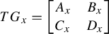 $$ \begin{align*} TG_x=\begin{bmatrix} A_x & B_x \\ C_x & D_x \end{bmatrix} \end{align*} $$
in which
 $|A_x| <\Vert DG_0|_{E^s}\Vert +\delta '$
,
 $|D_x^{-1}| < \Vert DG_0^{-1}|_{E^u}\Vert +\delta '$
, and
 $|B_x|, |C_x| < \delta '$
for some small
 $\delta ' $
uniformly on
 $V'$
, possibly shrinking
 $V'$
. Also, by possibly shrinking
 $V'$
, we may assume that the tangent directions to
 $\mathcal {F}$
can be written as the graph of a linear map from
 $F_x^u$
to
 $F_x^s$
(with operator norm bounded by
 $1$
on
 $V'$
).
We are now ready to describe how to use Theorem A.1. First, we make the following associations to fit into the terms of the statement:
 $V' \cap G^{-1}(V') \rightarrow U$
,
 $G \rightarrow h$
and
 $V' \rightarrow M$
. If
 $U \subset h(U)$
, then we are in the context of the usual
 $C^r$
section theorem and nothing needs to be done. Let E be the
 $C^2$
bundle whose fibers are
 $L(F_x^u,F_x^s)$
and so
 $m=2$
. Let D be the disk bundle of radius
 $C = 1$
. This bundle can be seen as trivial and equipped with the product metric through the addition of a trivializing complementary bundle, in a manner similar to that mentioned in the proof of Theorem A.1. The map F is defined by
 $F(x,T)=(x, \Gamma _{DF}(x)(T))$
, where
 $$ \begin{align*} \Gamma_{DF}(x)(T)= [B_x + A_x T]\circ[D_x + C_x T]^{-1} \end{align*} $$
for any
 $T \in L(F_x^u,F_x^s) $
. Notice
 $D_x + C_x T$
is invertible because it is very close to
 $D_x$
that is invertible (remember that the norm of T is bounded, as we are in the disk bundle D). The set N is as before. It is however necessary to check the construction of Pixton to see that it has the desired properties. The idea here is that N can be chosen very small around
 $\overline {W^{s}_{G,\alpha }\setminus G(W^{s}_{G,\alpha })}$
and V is constructed according to N. We associated to the foliation
 $\mathcal{F}^{\kern1pt u}_G$
the section
 $s=(x,T_x(\mathcal{F}^{\kern1pt u}_G))$
identifying these tangent spaces with the graph of a linear transformation. Observe that this section is invariant by F. So, if we write
 $s_0=s|_{N}$
, it is the unique invariant section guaranteed by Theorem A.1.
Given small
 $\delta ''>0$
, making
 $\delta \text { and } \delta '$
sufficiently small, we have that
 $\Gamma _{DF}$
is a fiber contraction of constant at most
 $ \Vert DG_0|_{E^s}\Vert \cdot \Vert DG_0^{-1}|_{E^u}\Vert + \delta ''$
. Given
 $\delta '''> 0$
, if we shrink
 $V'$
, the Lipschitz constant of the base map
 $G^{-1}$
is at most
 $ \Vert DG_0^{-1}|_{E^s}\Vert + \delta '''$
. Therefore, writing
 $r = 1+\varepsilon $
, for sufficiently small
 $\delta ''$
and
 $\delta '''$
,
 $$ \begin{align*} (\Vert DG_0|_{E^s}\Vert \cdot \Vert DG_0^{-1}|_{E^u}\Vert + \delta'') \cdot (\Vert DG_0^{-1}|_{E^s}\Vert + \delta''')^{r} < 1. \end{align*} $$
This is enough to show that the section
 $(x,T_x(\mathcal {F}\cup W^u))$
is the unique invariant section of the
 $C^r$
section theorem that agrees with
 $\mathcal {F}$
on N, and so it is
 $C^{1+\varepsilon }$
. By the same argument with the Fröbenius theorem, we can express the foliation
 $\mathcal {F}$
locally through a finite number of
 $C^1$
charts and the fact that the section above is
 $C^{1+\varepsilon }$
allows us to show that these charts are actually
 $C^{1+\varepsilon }$
. The continuity in the
 $C^{1 + \varepsilon }$
topology comes immediately from the construction and previous observations, we only require
 $\mathcal {F}_0$
and its derivatives to be uniformly continuous on V, which is clearly possible to be done.
Corollary A.5 With the hypothesis
 $\Vert DG_0|_{E^s}\Vert \cdot \Vert DG_0 |_{E^u}\Vert <1$
, the last theorem guarantees the existence of a
 $C^2$
foliation
 $\mathcal{F}^{\,u}_{G}$
for any G sufficiently close to
 $G_0$
.
This could be the case in the dissipative context, especially in the case of horseshoes arising from transversal homoclinic intersections.