2.1. Scaling and asymptotic regions

We consider the pressure-driven incompressible flow at the entrance of a pipe with circular cross-section. Dimensional quantities are hereafter indicated by the superscript $*$. The oncoming flow approaching the pipe entrance is assumed to be uniform, of velocity $U^*_\infty$ and aligned with the pipe axis. The pipe wall is assumed to be infinitely thin so that, similar to the case of uniform flow approaching a thin flat wall, the oncoming flow is undisturbed at leading order. In a laboratory, the upstream geometry and the finite thickness of the pipe wall may alter the uniformity of the oncoming flow. Our inlet flow, therefore, is a simplified version of that utilized by O. Reynolds in his seminal study (Reynolds Reference Reynolds1883), where the pipe entrance was bell shaped. As the oncoming flow enters the pipe, a boundary layer develops on the pipe wall. The thickness of this viscous layer increases downstream until the pipe flow becomes fully viscous and attains the classical Poiseuille parabolic profile.

The flow is conveniently represented in a cylindrical coordinate system, where the coordinates $x^*,r^*$ and $\theta$ are the streamwise direction, the radial direction and the azimuthal angle, respectively. The centreline of the pipe is at $r^*=0$ and the pipe wall is located at $r^*=R^*$, where $R^*$ is the pipe radius. Lengths are scaled by a reference length $\lambda ^*$, specified below. Velocities are normalized by $U^*_\infty$, the pressure is scaled by $\rho ^* U_\infty ^{*2}$, where $\rho ^*$ is the density of the fluid, and the time is scaled by $\lambda ^*/U^*_\infty$ (quantities without any symbols are non-dimensional).

Superimposed on the oncoming streamwise flow $\{U^*_\infty,0,0\}$ are gust-type vortical fluctuations advected by the base flow. In a technological or industrial system, these oncoming disturbances could be due to upstream vibrations or structural imperfections, and in a laboratory setting they could be generated by vibrating ribbons or rigid grids located near the pipe entrance, where the wavelengths and frequencies could be controlled accurately, as could the location of generation.

We first consider a region around the pipe axis where velocity fluctuations are not influenced by the pipe wall, either by the no-penetration condition on the radial velocity disturbance or by the no-slip condition on the streamwise and azimuthal velocity components. At these locations sufficiently near $x=0$ and sufficiently far away from the pipe wall, the velocity fluctuations can be expressed mathematically as a Fourier–Bessel series, where the Fourier expansions pertain to time, $x$ and $\theta$, while the Bessel expansion is used along the radial coordinate. As it is assumed that the amplitude of the perturbation is asymptotically smaller than $U^*_\infty$, the perturbation dynamics is linear. A single Fourier–Bessel coefficient of the full-spectrum series expansion is thus considered, as follows:

(2.1)\begin{equation} \boldsymbol{u}=\{1,0,0\}+ \varepsilon \left\{ \hat{u}_{x,m n}^\infty J_m (\bar{r}), \frac{\hat{u}_{r,m n}^\infty J_m (\bar{r})}{\bar{r}}, \frac{-\textrm{i} \hat{u}_{\theta,m n}^\infty J'_m(\bar{r})}{\xi_{m n}} \right\} \textrm{e}^{\textrm{i}[k_x (x-t) + m \theta]} +\text{c.c.}, \end{equation}

where $J_m$ is the Bessel function of the first kind of order $m$, $E=\textrm {e}^{\textrm {i}[k_x (x-t) + m \theta ]}$, $\varepsilon \ll 1$ is the amplitude of the gust, $\bar {r}=\xi _{m n}r/2R$, $\xi _{m n}$ are the zeros of the Bessel function, i.e. the real numbers that satisfy $J_m(\xi _{m n})=0$, c.c. stands for the complex conjugate, and the prime indicates the first derivative with respect to $\bar {r}$. In the most general case, the quantities $\{\hat {u}_{x,jm n}^\infty,\hat {u}_{r,jm n}^\infty,\hat {u}_{\theta,jm n}^\infty \}=O(1)$ are complex. The inviscid velocity field (2.1) satisfies the Euler equations and is generated at a circle of radius $2R$, centred at the pipe centreline and located in the plane $(r,\theta )$ at a small distance upstream of the pipe mouth at $x=0$. The scaling of the radial direction by $2R$ is used instead of $R$ to avoid the unrealistic scenario of vanishing streamwise and radial velocity components at $r=R$ where the disturbance is generated.

The reference length is $\lambda ^*=\theta _g R^*$ ($\lambda ^*/R^* = O(1)$), that is, the circumferential wavelength of the gust at $r^*=R^*$, where $\theta _g$ is the azimuthal angle corresponding to the wavelength $\lambda ^*$. As in the flat-plate case of Leib, Wundrow & Goldstein (Reference Leib, Wundrow and Goldstein1999) where the spanwise wavelength is used, the azimuthal wavelength $\lambda ^*$ at $r^*=R^*$ is chosen because downstream it becomes comparable with the boundary layer thickness and the pipe radius. If $\theta _g={\rm \pi} /2$, the wavelength $\lambda ^*$ spans a quarter of the circumference of the pipe. An obvious constraint is that the maximum $\lambda ^*$ coincides with the pipe circumference. The coefficient $m=2{\rm \pi} R \in \mathbb {N}$ denotes the number of wavelengths $\lambda ^*$ around the circumference (we restrict ourselves to cases for which $m\neq 0$ because we are interested in three-dimensional disturbances). The radial velocity is never singular at the centreline despite $J_m$ being divided by $\bar {r}$ because, given $J_m(\bar {r}) \sim (\bar {r}/2)^m/\varGamma (m+1)$ for $\bar {r}\ll 1$ (where $\varGamma$ is the gamma function), the radial average $\hat {u}_{r,0n}^\infty$ is zero.

The focus is on low-frequency (i.e. long wavelength) disturbances with a streamwise wavenumber $k_x=2{\rm \pi} \lambda ^*/\lambda _x^* \ll 1$, where $\lambda _x^*$ is the streamwise wavelength of the gust, as these perturbations are most likely to penetrate a boundary layer and generate laminar streaks (Matsubara & Alfredsson Reference Matsubara and Alfredsson2001). As the convected gust is transported passively by the uniform base flow, the pressure fluctuations are negligible at leading order in $k_x \ll 1$ (refer to Goldstein (Reference Goldstein1978, (2.3)) and Leib et al. (Reference Leib, Wundrow and Goldstein1999, (3.2))). Equation (2.1) satisfies the continuity equation as the term emerging from $\partial u / \partial x$ is $O(k_x) \ll 1$, i.e.

(2.2)\begin{equation} \xi_{m n} \hat{u}_{r,m n}^\infty + m \hat{u}_{\theta,m n}^\infty=O(k_x). \end{equation}

Without losing generality, $m>0$ is taken. The continuity equation also determines the $\bar {r}^{-1}$ dependence for the radial velocity and the dependence on the derivative of the Bessel function and the coefficient $-\textrm {i}/\xi _{mn}$ for the the azimuthal velocity.

The Reynolds number is $Re_\lambda =U_{\infty }^*\lambda ^*/\nu ^* \gg 1$. Inside the pipe, the disturbances evolve downstream on a length scale that is comparable with the streamwise gust wavelength. A distinguished scaling is thus $k_x=O(Re_\lambda ^{-1})$ or $\bar {x}=k_x x=2{\rm \pi} x^*/\lambda _x^*=O(1)$. The disparity between the streamwise and azimuthal scales implies that disturbances of amplitude $O(\varepsilon )$ may generate streamwise velocity perturbations with an amplitude of $O(\varepsilon /k_x)$ in the viscous layers. These amplitudes are assumed to be much smaller than $U^*_\infty$, which translates to $\varepsilon /k_x \ll 1$ or $\varepsilon Re_\lambda \ll 1$ and implies that the Navier–Stokes equations may be linearized.

Vortical disturbances analogous to those defined in (2.1) have been found in other cylindrical flows, i.e. the instability modes of a rotating pipe flow also have the streamwise velocity component proportional to $J_m$ and the radial velocity proportional to $J_m/r$ (Pedley Reference Pedley1969). A similar choice for the oncoming disturbance was employed for the flat-plate boundary-layer cases studied by Ricco, Luo & Wu (Reference Ricco, Luo and Wu2011) and Marensi, Ricco & Wu (Reference Marensi, Ricco and Wu2017), who prescribed the vorticity fluctuations as a pair of gusts with equal and opposite spanwise wavenumbers. Disturbances (2.1) are physically realistic because they may be generated, for example, by a grid at the entry of the pipe, as a circular analogue to the vibrating wires used in the receptivity studies by Dietz (Reference Dietz1999) and Borodulin et al. (Reference Borodulin, Ivanov, Kachanov and Roschektayev2021a,Reference Borodulin, Ivanov, Kachanov and Roschektayevb) for two- and three-dimensional free stream vortical disturbances, respectively.

As shown in figure 1, the domain is divided into six asymptotic regions. The effect of the base-flow streamwise pressure gradient is negligible in regions I, II and III, mild in region IV, and fully influential in region V. In region VI, the base flow is fully developed. In region I, at $x=O(1)$, the base and the perturbation flows are inviscid and rapid distortion theory applies (Goldstein Reference Goldstein1978). A velocity potential is used and the wall is taken into account through the no-penetration condition on the radial velocity component. In the viscous region II, $\delta ^*/\lambda ^* \ll 1$, where $\delta ^*$ is the boundary-layer thickness. Regions I and II are studied in § 3.2.1. Region III occurs where $\delta ^*/\lambda ^*=O(1)$ and $\bar {x}=O(1)$ and it is governed by the linearized unsteady boundary-region equations (Leib et al. Reference Leib, Wundrow and Goldstein1999). In region IV, which is in the pipe core and surrounded by region III, the base flow is inviscid and the perturbation flow is viscous. Regions III and IV are discussed in § 3.2.2. In region V the base flow is not self-similar because of the unknown pressure gradient. The streamwise base-flow velocity at the pipe axis increases with $x$ and the base flow is non-parallel as the radial velocity plays a key role. The latter vanishes farther downstream in region VI, where the parabolic Poiseuille profile occurs.

Figure 1.

Asymptotic regions of the pipe flow (not in scale). The boundary-layer thickness $\delta _R$ is defined in § 4.1.

2.2. Governing equations and boundary conditions

The flow field is governed by the continuity and Navier–Stokes equations,

(2.3)$$\begin{gather} \boldsymbol{\nabla} \boldsymbol{\cdot} \boldsymbol{u} =0, \end{gather}$$

(2.4)$$\begin{gather}\frac{\partial \boldsymbol{u}}{\partial t}+(\boldsymbol{u}\boldsymbol{\cdot} \boldsymbol{\nabla})\boldsymbol{u} ={-}\boldsymbol{\nabla} p+\frac{1}{Re_\lambda}\nabla^2 \boldsymbol{u}, \end{gather}$$

where $\boldsymbol {u}=\{ u_x,u_r,u_\theta \}$. The velocity $\boldsymbol {u}$ and the pressure $p$ are expressed as the superposition of the base flow and the perturbation flow, i.e. $\{\boldsymbol {u},p\}=\{\bar {\boldsymbol {U}}(\bar {x},r), \bar {P}(\bar {x})\} +\{\boldsymbol {u}',p'\}$, where

(2.5)$$\begin{gather} \{\bar{\boldsymbol{U}}(\bar{x},r), \bar{P}(\bar{x})\}= \{ U(\bar{x},r), k_xV(\bar{x},r), 0, P(\bar{x}) \}, \end{gather}$$

(2.6)$$\begin{gather}\{\boldsymbol{u}',p'\}=\{u',v',w',p'\}= \varepsilon \begin{pmatrix} \bar{u}_{x,0}(\bar{x},r)\\ \bar{u}_{r,0}(\bar{x},r)\\ \bar{u}_{\theta,0}(\bar{x},r) \\ \bar{p}_0(\bar{x},r) \end{pmatrix} \textrm{e}^{\textrm{i}(m \theta - k_x t)} + \text{c.c.} \end{gather}$$

and

(2.7a)$$\begin{gather} \{ \bar{u}_{x,0}, \bar{u}_{r,0}\} = \{ \bar{u}_x^{(0)}, k_x \bar{u}_r^{(0)}\} + \left\{\frac{\textrm{i} m}{k_x}\bar{u}_x, \textrm{i} m\bar{u}_r\right\}, \end{gather}$$

(2.7b)$$\begin{gather}\bar{u}_{\theta,0} ={-} \frac{\textrm{i} k_x}{m}\bar{u}_\theta^{(0)} + \bar{u}_\theta, \end{gather}$$

(2.7c)$$\begin{gather}\bar{p}_0 = \frac{k_x}{Re_\lambda} \bar{p}^{(0)} + \frac{\textrm{i} m}{Re_\lambda} \bar{p}. \end{gather}$$

The notation in (2.6)–(2.7) is as close as possible to the flat-plate case by Leib et al. (Reference Leib, Wundrow and Goldstein1999) for ease of understanding. The main difference between $\bar {u}_r$ and $\bar {u}_r^{(0)}$ and the corresponding components in (4.1) on page 176 of Leib et al. (Reference Leib, Wundrow and Goldstein1999) is the missing factor $(2 \bar {x})^{1/2}$ in (2.6), which arises in Leib et al. (Reference Leib, Wundrow and Goldstein1999)'s case because of the Blasius-similarity scaling.

By substituting (2.5)–(2.6) into (2.3)–(2.4) and collecting the terms of $O(1)$, one obtains the base-flow boundary-layer equations (Hornbeck Reference Hornbeck1964),

(2.8)$$\begin{gather} \frac{\partial U}{\partial \bar{x}} + \frac{V}{r} + \frac{\partial V}{\partial r} =0, \end{gather}$$

(2.9)$$\begin{gather}U\frac{\partial U}{\partial \bar{x}} + V \frac{\partial U}{\partial r}={-}\frac{\rm{d}P}{\rm{d}\bar{x}}+\frac{1}{\mathcal{F}}\left( \frac{1}{r} \frac{\partial U}{\partial r}+\frac{\partial^2 U}{\partial r^2} \right ), \end{gather}$$

(2.10)$$\begin{gather}\frac{\partial P}{\partial r}=0, \end{gather}$$

for $k_x, Re_\lambda ^{-1} \ll 1$ and $\mathcal {F} = k_x Re_\lambda = O(1)$. As $P$ is unknown, (2.8)–(2.9) are solved together with the mass conservation law, $\int _0^R U r \,\rm {d}r = R^2/2$, found by averaging across a pipe cross-section. Equations (2.8) and (2.9) are subject to the no-slip and no-penetration conditions at the pipe wall, $U=V=0$ at $r=R$, and to the symmetry conditions at the axis, $\partial U/\partial r=V=0$ at $r=0$. As $p'$ at the wall is unknown, we eliminate the pressure from (2.3)–(2.4) (Kim, Moin & Moser Reference Kim, Moin and Moser1987) to obtain the perturbation-flow equations,

(2.11)$$\begin{gather} \hat V \bar{u}_r + \hat V_r \frac{\partial \bar{u}_r}{\partial r} + \hat V_{rr} \frac{\partial^2 \bar{u}_r}{\partial r^2} + \hat V_{rrr} \frac{\partial^3 \bar{u}_r}{\partial r^3} + \hat V_{rrrr} \frac{\partial^4 \bar{u}_r}{\partial r^4} + \hat V_x \frac{\partial \bar{u}_r}{\partial \bar{x}} + \hat V_{xr} \frac{\partial^2 \bar{u}_r}{\partial \bar{x}\partial r} + \hat V_{xrr} \frac{\partial^3 \bar{u}_r}{\partial \bar{x}\partial r^2} \nonumber\\ + \hat U \bar{u}_x + \hat U_r \frac{\partial \bar{u}_x}{\partial r} + \hat U_{rr} \frac{\partial^2 \bar{u}_x}{\partial r^2} + \hat U_x \frac{\partial \bar{u}_x}{\partial \bar{x}} + \hat U_{xr} \frac{\partial^2 \bar{u}_x}{\partial \bar{x}\partial r} + \hat U_{xrr} \frac{\partial^3 \bar{u}_x}{\partial \bar{x}\partial r^2} =0, \end{gather}$$

(2.12)$$\begin{gather}\left(-\textrm{i}+ \frac{m^2}{\mathcal{F} r^2}+ \frac{\partial U}{\partial \bar{x}} \right) \bar{u}_x + \left(V - \frac{1}{\mathcal{F} r} \right) \frac{\partial \bar{u}_x}{\partial r} + U \frac{\partial \bar{u}_x}{\partial \bar{x}} - \frac{1}{\mathcal{F}}\frac{\partial^2 \bar{u}_x}{\partial r^2} + \frac{\partial U}{\partial r}\bar{u}_r=0. \end{gather}$$

The coefficients of (2.11) are

(2.13)$$\begin{gather} \hat V = \left( \frac{1}{m^2} -1 \right) \left( \boxed{\textrm{i}} - \frac{\partial V}{\partial r} + \frac{1 - m^2}{\mathcal{F} r^2} \right) + \frac{2 r}{m^2} \frac{\partial^2 U}{\partial r \partial \bar{x}} + \frac{r^2}{m^2} \frac{\partial^3 U}{\partial r^2 \partial \bar{x}}, \end{gather}$$

(2.14)$$\begin{gather}\hat V_r = \boxed{\frac{3 \textrm{i} r}{m^2}} - \frac{3 r}{m^2} \frac{\partial V}{\partial r} - \frac{1}{\mathcal{F} r m^2} - \frac{2}{\mathcal{F} r} + V - \frac{4 V}{m^2} + \frac{r^2}{m^2} \frac{\partial^2 U}{\partial r \partial \bar{x}}, \end{gather}$$

(2.15)$$\begin{gather}\hat V_{rr} = \frac{1}{m^2} \left(\boxed{\textrm{i}r^2} - 5 r V - r^2 \frac{\partial V}{\partial r} - \frac{2 m^2}{\mathcal{F}} + \frac{5}{\mathcal{F}} \right) \end{gather}$$

(2.16)$$\begin{gather}\hat V_{rrr} = \frac{1}{m^2} \left( \frac{6 r}{\mathcal{F}} - r^2 V \right), \end{gather}$$

(2.17)$$\begin{gather} \hat V_{rrrr} = \frac{r^2}{\mathcal{F} m^2}, \end{gather}$$

(2.18)$$\begin{gather}\hat V_x = U - \frac{U}{m^2} + \frac{r}{m^2} \frac{\partial U}{\partial r} + \frac{r^2}{m^2} \frac{\partial^2 U}{\partial r^2}, \end{gather}$$

(2.19)$$\begin{gather}\hat V_{xr} ={-} \frac{3 r U}{m^2}, \end{gather}$$

(2.20)$$\begin{gather}\hat V_{xrr} ={-}\frac{r^2 U}{m^2}, \end{gather}$$

(2.21)$$\begin{gather}\hat U = \frac{\partial V}{\partial \bar{x}} + \frac{2 r}{m^2} \frac{\partial^2 U}{\partial \bar{x}^2} + \frac{r^2}{m^2} \frac{\partial^3 U}{\partial \bar{x}^2\partial r}, \end{gather}$$

(2.22)$$\begin{gather}\hat U_x ={-}\frac{2}{\mathcal{F} r} + \frac{6 r}{m^2} \frac{\partial U}{\partial \bar{x}} + \frac{2 r^2}{m^2} \frac{\partial^2 U}{\partial \bar{x} \partial r}, \end{gather}$$

(2.23)$$\begin{gather}\hat U_r = \frac{r}{m^2} \frac{\partial V}{\partial \bar{x}}, \end{gather}$$

(2.24)$$\begin{gather}\hat U_{rr} = \frac{r^2}{m^2} \frac{\partial V}{\partial \bar{x}}, \end{gather}$$

(2.25)$$\begin{gather}\hat U_{xr} = \frac{2}{m^2} \left(\frac{1}{\mathcal{F}} - 2 r V - r^2 \frac{\partial V}{\partial r} \right), \end{gather}$$

(2.26)$$\begin{gather}\hat U_{xrr} = \frac{2 r}{m^2 \mathcal{F}}. \end{gather}$$

The boxed terms in (2.13)–(2.15) pertain to the unsteadiness and are asymptotically smaller than the other terms in the low-frequency limit $\mathcal {F} \ll 1$. The procedure to obtain (2.11)–(2.12) is given in the supplementary material S2. Equations (2.11) and (2.12) are also satisfied by $\{\bar {u}_x^{(0)},\bar {u}_r^{(0)}\}$. At the start of the analysis, (2.12) is the radial vorticity equation, but it reduces to the $x$-momentum equation because the leading-order contribution to the radial vorticity is given by $\bar {u}_x$ due to $k_x \ll 1$. Equations (2.11) and (2.12) are subject to

(2.27)\begin{equation} \bar{u}_x=\bar{u}_r=\frac{\partial \bar{u}_r}{\partial r}=0 \end{equation}

at $r=R$ because of the no-slip condition at the pipe wall and the continuity equation (S2.5). The boundary conditions at $r=0$ are

(2.28)$$\begin{gather} m=1: \quad \bar{u}_x=0, \quad \bar{u}'_r=0, \quad \bar{u}_\theta'=0, \end{gather}$$

(2.29)$$\begin{gather}m=2: \quad \bar{u}_x=0, \quad \bar{u}_r=0, \quad \bar{u}_\theta=0, \end{gather}$$

(2.30)$$\begin{gather}m>2: \quad \bar{u}_x=0, \quad \bar{u}_r=0, \quad \bar{u}_r'=0, \end{gather}$$

where the prime here indicates the derivative with respect to $r$. For $m=1$, (2.11)–(2.12) are solved together with the continuity equation (S2.5) because $\bar {u}_\theta$ appears in (2.28). For $m=2$, this complication is avoided by using $\bar {u}_r''=0$ instead of the last condition in (2.29). The behaviour of the perturbation flow near the pipe axis and the derivation of the boundary conditions is further discussed in the supplementary material S3. The same boundary conditions are found for $\bar {u}^{(0)}_x,\bar {u}^{(0)}_r,\bar {u}^{(0)}_\theta$. The azimuthal velocity component $\bar {u}_\theta$ and the pressure $\bar {p}$ are computed a posteriori from the continuity equation (S2.5) and the azimuthal momentum equation (S2.8).

The base-flow equations (2.8)–(2.9) and the perturbation (2.11)–(2.12) are parabolic and thus the specification of the appropriate initial conditions is of crucial importance. We have devoted great attention to the formulation of physically meaningful initial conditions for both the base flow and the perturbation flow. The initial base-flow velocity profile has usually been assumed uniform (Hornbeck Reference Hornbeck1964). We instead take into account the interaction between the oncoming flow and the pipe wall by deriving an asymptotic solution composed of the Blasius flow near the walls (inner solution) and the inviscid flow in the pipe core, distorted by the developing boundary layers (outer solution). The supplementary material S4 discusses the conditions under which the curvature effects can be neglected near the wall. The small-$x$ base-flow asymptotic initial condition used to solve the base-flow equations (2.8)–(2.9) is described in § 3.1.

Perturbation inflow conditions for open boundary-layer computations are often specified as the continuous spectrum of the Orr–Sommerfeld equations (Jacobs & Durbin Reference Jacobs and Durbin2001; Brandt, Schlatter & Henningson Reference Brandt, Schlatter and Henningson2004) or by selecting optimal perturbations, as those obtained for the flat-plate case by Andersson, Berggren & Henningson (Reference Andersson, Berggren and Henningson1999) and Luchini (Reference Luchini2000). As inflow conditions, Buffat et al. (Reference Buffat, Le Penven, Cadiou and Montagnier2014) imposed optimal disturbances within one of the boundary layers near the entrance of a channel, while perturbations were absent in the inviscid core.

We prescribe initial conditions that are superposed on the inviscid core flow and match the oncoming vortical disturbances at $\bar {x}=0$, given in (2.1). Like the base flow, these initial conditions are expressed as asymptotic composite solutions of a viscous inner solution within the boundary layer and an outer solution where the base flow is inviscid in the pipe core because we are interested in their entrainment of vortical disturbances that occupy the entire cross-plane near the pipe mouth. The initial condition is not imposed at $\bar {x}=0$ because the radial base-flow velocity is singular there and because the flow field is governed by the full Navier–Stokes equations in the immediate surroundings of the inlet. Therefore, the initial conditions are imposed at a location $0 < \bar {x}_0 \ll 1$.

Section 3.2 presents results for the development of the perturbation flow at small-$\bar {x}$ locations where the base-flow pressure gradient is negligible. These flow fields are small-$\bar {x}$ asymptotic solutions of the flow in region V and can therefore be used as initial conditions to solve equations (2.11)–(2.12) along the pipe, where the base-flow streamwise pressure gradient is fully influential.

2.3. Critical streamwise location for linear stability

As we are interested in the spatial transient growth of vortical disturbances in the entrance region, a first step is to report, as a function of the Reynolds number, the streamwise locations where TS waves appear. Figure 2 shows the neutral stability locations $x_c/R$ as a function of the Reynolds number $Re_R=R Re_\lambda =U^*_\infty R^*/\nu ^*$ computed by Gupta & Garg (Reference Gupta and Garg1981) (blue line) and da Silva & Moss (Reference da Silva and Moss1994) (red circles). The entrance flow is linearly stable for $Re_R<11\,000$ and the unstable region has a finite extent along the $x$ direction as the flow is always linearly stable when it reaches the fully developed condition. We also show the experimental neutral points by Sarpkaya (Reference Sarpkaya1975), measured by introducing disturbances at fixed locations on the pipe wall by electromagnetic excitation. da Silva & Moss (Reference da Silva and Moss1994) claimed that the disagreement may be due to the finite amplitude of Sarpkaya (Reference Sarpkaya1975)'s perturbations, which cannot be captured by the linear stability theory. We focus on Reynolds numbers in the range $1000< Re_R<10\,000$ (marked by the light grey area in figure 2), i.e. small enough for TS waves not to appear and large enough for algebraically growing perturbations or transition to turbulence to have been observed in experimental studies.

Figure 2.

The blue line and red circles confine the unstable area according to classical stability theory, i.e. where TS waves start to grow, computed by Gupta & Garg (Reference Gupta and Garg1981) and da Silva & Moss (Reference da Silva and Moss1994), respectively. The black (axisymmetric disturbances) and white (non-axisymmetric disturbances) circles represent the experimental neutral points measured by Sarpkaya (Reference Sarpkaya1975). The solid black line denotes the end location of the entry pipe-flow region, according to our definition based on the second derivative of the base velocity at the centreline, discussed in § 4.1. The grey area illustrates the range of Reynolds numbers for the flows studied.

3.1. Initial base flow in regions I and II

The initial base-flow solution is constructed according to the method of matched asymptotic expansions. The outer solution is the inviscid base flow in the core of the pipe, while the inner solution is the viscous flow attached to the pipe wall. The composite solution reads

(3.1)\begin{equation} \bar{\boldsymbol{U}}=\bar{\boldsymbol{U}}_{out}+\bar{\boldsymbol{U}}_{in}-\bar{\boldsymbol{U}}_{com}, \end{equation}

where the subscripts in, out and com stand for inner, outer and common, respectively, and $\bar {\boldsymbol {U}}$ is defined in (2.5). The common part is defined as

(3.2)\begin{equation} \bar{\boldsymbol{U}}_{com}=\lim_{r \rightarrow R} \bar{\boldsymbol{U}}_{out}=\lim_{\eta \rightarrow \infty} \pm \bar{\boldsymbol{U}}_{in}, \end{equation}

where

(3.3)\begin{equation} \eta=(R-r)\left( \frac{Re_\lambda}{2 x}\right)^{1/2}=O(1) \end{equation}

is the scaled radial coordinate of the inner solution and in (3.2) the plus sign applies to the streamwise velocity and the minus sign applies to the radial velocity because the coordinates $r$ and $\eta$ point in opposite directions.

For the flow in the entrance region of a channel, the inner solution near the inlet corresponds to the Blasius flow as the Reynolds number is large (Wilson Reference Wilson1970; Rubin, Khosla & Saari Reference Rubin, Khosla and Saari1977; Duck Reference Duck2005; Buffat et al. Reference Buffat, Le Penven, Cadiou and Montagnier2014). We also benefit from the Blasius solution in the pipe-flow case as we have proved in the supplementary material S4 that the curvature effects are negligible near the wall. The inner flow therefore satisfies the self-similar Blasius equation

(3.4)\begin{equation} F'''+FF''=0, \end{equation}

where the prime indicates differentiation with respect to $\eta$. The boundary conditions for (3.4) are $F(0)=0$, $F'(0)=0$ and $F'\rightarrow 1$ as $\eta \rightarrow \infty$. The inner base flow reads

(3.5)\begin{equation} \bar{U}_{in}=F', \quad \bar{V}_{in}=\frac{\eta F' - F}{(2 x Re_\lambda)^{1/2}}. \end{equation}

As $Re_\lambda \gg 1$, the base-flow viscous effects are negligible in the pipe core near the entrance, which is consistent with the use of the boundary-layer approximation of the Navier–Stokes equations. In the pipe core, the axisymmetric outer flow is described by the inviscid Stokes stream function $\psi$,

(3.6)\begin{equation} \psi(x,r)=\frac{r^2}{2}+Re_\lambda^{{-}1/2}\psi_2(x,r), \end{equation}

i.e. $\bar {U}_{out}=r^{-1}\partial \psi /\partial r$ and $\bar {V}_{out}=-r^{-1}\partial \psi /\partial x$. The leading-order term $r^2/2$ in (3.6) represents the uniform streamwise flow. The second-order stream function $\psi _2$, which defines the flow due to the pipe confinement and to the Blasius boundary layer developing on the pipe wall, satisfies

(3.7)\begin{equation} \frac{\partial^2 \psi_2}{\partial x^2} + \frac{\partial^2 \psi_2}{\partial r^2} - \frac{1}{r} \frac{\partial \psi_2}{\partial r} =0, \end{equation}

subject to

(3.8a)$$\begin{gather} \psi_2 =\beta R \sqrt{2x} \quad \rm{at} \ r=R,\ x>0, \end{gather}$$

(3.8b)$$\begin{gather}\psi_2 =0 \quad \rm{at} \ r=R, x<0, \end{gather}$$

(3.8c)$$\begin{gather}\psi_2 =0 \quad \rm{at} \quad r=0, \end{gather}$$

where $\beta =\lim _{\eta \rightarrow \infty } (\eta - F) =1.217 \ldots\, $. The inviscid base flow in the pipe core is irrotational and therefore the governing equation (3.7) is obtained by setting the azimuthal vorticity component to zero. Equation (3.7) is not the Laplace equation because of the negative sign of the last term (Panton Reference Panton2013). The boundary condition (3.8a) is obtained by asymptotic matching, i.e. the radial component of the outer velocity must match the outer limit of the base-flow wall-normal velocity of the Blasius boundary layer,

(3.9)\begin{align} \bar{V}_{com} &= \lim_{r \rightarrow R} \bar{V}_{out}= \frac{-1}{RRe_\lambda^{1/2}}\left.\frac{\partial \psi_2}{\partial x}\right\rvert_{r=R} ={-}\lim_{\eta \rightarrow \infty} \bar{V}_{in}\nonumber\\ &= \lim_{\eta \rightarrow \infty} \frac{F-\eta F'}{(2 x Re_\lambda)^{1/2}} = \frac{-\beta}{ ({2 x Re_\lambda} )^{1/2}}, \end{align}

where the minus sign in front of the $\eta$-limit is due to the inner and outer velocity components pointing towards opposite directions. It follows that

(3.10)\begin{equation} \psi_2(x)=\beta R \int (2 x)^{{-}1/2}\,\rm{d}x=\beta R \sqrt{2x}, \end{equation}

at $r=R$ for $x>0$. The boundary condition (3.8b) is obtained as follows. The base flow is uniform and streamwise only as $x \rightarrow -\infty$ and, as it is not influenced by the presence of the pipe, no wall-normal base-flow velocity occurs as $x \rightarrow -\infty$. Also, the horizontal line $r=R$ for $x<0$ is a streamline with stagnation point at $x=0^-,r=R$ and no wall-normal base-flow velocity occurs along it because the base flow approaches the pipe wall parallel to it. Therefore, $\bar {V}_{out}=0$ at $r=R$ for $x<0$, i.e. $\partial \psi / \partial x=\partial \psi _2 / \partial x=0$. As we choose $\psi _2=0$ as $x \rightarrow -\infty$, by integrating $\partial \psi _2 / \partial x=0$ from $x \rightarrow -\infty$ for $r=R$, it follows that $\psi _2=0$ along $r=R$ for $x<0$. The boundary condition (3.8c) follows from $\bar {V}_{out}=0$ along the pipe axis at any $x$ due to the flow axial symmetry.

The solution to (3.7) together with the boundary conditions (3.8) is found by use of the complex Fourier transform along $x$. The solution reads

(3.11)\begin{equation} \psi_2(x,r)={-}\frac{r\beta \textrm{i}^{1/2}}{2 \sqrt{2 {\rm \pi}}} \int_{-\infty+\textrm{i} \gamma}^{+\infty+\textrm{i} \gamma} \frac{I_1(\zeta r)\, \textrm{e}^{\textrm{i}\zeta x}}{I_1(\zeta R) \zeta^{3/2}} \,\mathrm{d}\zeta, \end{equation}

where $I_1$ is the modified Bessel function of the first kind and $\gamma \in \mathbb {R}<0$. The supplementary material S5 presents the derivation of (3.11) (Dettman Reference Dettman1965). The composite solution of the streamwise velocity $U$ is

(3.12)\begin{align} U(x,r)&=\bar{U}= F'(\eta(x,r)) -\frac{\beta \textrm{i}^{1/2}}{2 \sqrt{2 {\rm \pi}}Re_\lambda^{1/2}} \int_{-\infty+\textrm{i} \gamma}^{+\infty+\textrm{i} \gamma} \frac{\textrm{e}^{\textrm{i}\zeta x}}{\zeta^{1/2} I_1(\zeta R)} \left[ \frac{I_1(\zeta r)}{\zeta r} + I_1^\prime(\zeta r) \right] \mathrm{d}\zeta \nonumber\\ &\quad +\frac{\beta \textrm{i}^{1/2}}{2 \sqrt{2 {\rm \pi}}Re_\lambda^{1/2}} \int_{-\infty+\textrm{i}\gamma}^{+\infty+\textrm{i} \gamma} \frac{\textrm{e}^{\textrm{i}\zeta x}}{\zeta^{1/2}} \left[ \frac{I_1^\prime(\zeta R)}{I_1(\zeta R)} + \frac{1}{\zeta R} \right] \mathrm{d}\zeta. \end{align}

The composite solution of the radial velocity $V$, defined in (2.5), is

(3.13)\begin{align} V(x,r)&=k_x^{{-}1} \bar{V} = \frac{\eta F'(\eta(x,r)) - F(\eta(x,r))}{k_x(2 x Re_\lambda)^{1/2}}\nonumber\\ &\quad + \frac{\beta \textrm{i}^{3/2}}{2 \sqrt{2 {\rm \pi}}k_x{Re}_{\lambda}^{1/2}} \int_{-\infty+\textrm{i} \gamma}^{+\infty+\textrm{i} \gamma} \frac{I_1(\zeta r) \,\textrm{e}^{\textrm{i}\zeta x}}{I_1(\zeta R) \zeta^{1/2}}\, \mathrm{d}\zeta + \frac{\beta}{k_x ({2 x Re_\lambda})^{1/2}}. \end{align}

Figure 3 shows the inner and outer solutions, their common parts, and the composite solutions for the base flow for $Re_\lambda =500$ and $2000$ at $x=0.04$. The composite base-flow streamwise velocity, depicted in figure 3(a,b), agrees well with the inner Blasius solution across the pipe radius as the acceleration in the pipe core is still small at this $x$ location. The increase of inviscid streamwise velocity balances the decrease within the viscous region to conserve the mass flow rate. The displacement effect of the Blasius boundary layers, given by (3.9), causes a small streamwise pressure gradient related to the dependence of the displacement stream function $\psi _2$ on the $x$ coordinate. This small pressure gradient is negligible at leading order in the boundary layer. The inviscid streamwise velocity is larger than unity near the wall because it accelerates along $x$ to conserve the mass flow rate as the radial velocity decreases from its boundary-layer blowing value as the pipe axis is approached. This acceleration gives rise to the local near-wall peak in the $\bar {U}$ profile, also reported in Durst et al. (Reference Durst, Ray, Ünsal and Bayoumi2005) for entry-pipe flow and in Sparrow, Lin & Lundgren (Reference Sparrow, Lin and Lundgren1964), Panton (Reference Panton2013) and Alizard et al. (Reference Alizard, Cadiou, Le Penven, Di Pierro and Buffat2018) for entry-channel flows. The peak occurs because the inviscid streamwise velocity is larger than the viscous streamwise velocity deficit of the boundary layer.

Figure 3.

Composite solutions for the base-flow streamwise velocity $\bar {U}$ (a,b) and radial velocity $\bar {V}$ (c,d) at $x=0.04$ for $R=1$ and two Reynolds numbers.

The base-flow radial velocity, shown in figure 3(c,d), agrees well with the viscous solution only in the proximity of the wall, while the two fail to overlap in the inviscid core, where the composite profile coincides with the outer solution. The composite solution shows a distinct near-wall peak that moves closer to the wall and decreases in intensity as the Reynolds number increases. The velocity is not exactly zero at the wall. This small slip velocity decreases as $O(Re_\lambda ^{-1/2})$ and induces a viscous layer at the next order, which is not computed.

3.2. Initial perturbation flow

The precise flow specification at the pipe entrance is relevant as our interest lies in the mathematical description of the inlet profiles to start the computations and to understand how the vortical disturbances are entrained in the pipe mouth and how they evolve in the entrance region. The initial perturbation flow, fully influenced by the confinement of the pipe and only mildly by the base-flow streamwise pressure, is studied in this section via matched asymptotic expansions. Asymptotic composite solutions are derived for regions I and II in § 3.2.1. The flow in regions III and IV is discussed in § 3.2.2.

3.2.1. Perturbation flow in regions I and II

In region I the base flow is uniform and inviscid, the perturbation flow is inviscid, and $\bar {x}\ll 1$ with $\mathcal {F}=O(1)$. The flow field can thus be adequately described by rapid distortion theory (Goldstein Reference Goldstein1978). The velocity is expressed as

(3.14)\begin{align} \boldsymbol{u}_{out} &= \hat{\boldsymbol{i}} + \varepsilon [\boldsymbol{u}^{(1)}(\bar{x},r) + k_x \boldsymbol{u}^{(1)}_1(\bar{x},r)]\, \textrm{e}^{\textrm{i}(m\theta-k_x t)}+ \text{c.c.} \nonumber\\ &=\hat{\boldsymbol{i}} + \varepsilon ( \boldsymbol{u}_\infty + \boldsymbol{\nabla} \phi + k_x \boldsymbol{\nabla} \phi_1) + \text{c.c.} \end{align}

The velocity $\boldsymbol {u}^{(1)}$ is due to the interaction of the free stream gust (2.1) with the pipe wall, while $\boldsymbol {u}^{(1)}_1$ is generated by the wall-normal boundary-layer perturbation velocity via $\boldsymbol {\nabla } \phi _1$. The perturbation potential $\phi$ satisfies the Laplace equation

(3.15)\begin{equation} \frac{1}{r}\frac{\partial}{\partial r} \left(r \frac{\partial\phi}{\partial r} \right)+ \frac{1}{r^2}\frac{\partial^2 \phi}{\partial \theta^2}+ \frac{\partial^2 \phi}{\partial x^2}=0, \end{equation}

subject to

(3.16a)$$\begin{gather} \phi \ \text{finite} \quad \text{at} \ r=0, \end{gather}$$

(3.16b)$$\begin{gather}\frac{\partial \phi}{\partial r}+u_{\infty r} = 0 \quad \text{at} \ r=R, \ x>0, \end{gather}$$

where $u_{\infty r}(r=R)= [2 \hat u^\infty _{r,mn} J_m(\xi _{mn}/2)/\xi _{mn}] \exp [\textrm {i} k_x (x-t) + \textrm {i} m \theta ]$ is the gust radial velocity found from (2.1) as the pipe wall is approached. Expression (3.16b) is the no-penetration boundary condition at the wall for the radial velocity. To solve (3.15) in the infinite strip $-\infty < x<\infty$, $0\leq r\leq R$, one needs a boundary condition at $r=R$ for $x<0$, which is unknown. However, the interest here is in the solution at $x \gg 1$, which can be found by separation of variables. In this limit, it is found that $\phi = \hat \phi (r) \exp [\textrm {i} k_x (x-t) + \textrm {i} m \theta ]$, where $\hat \phi (r)$ satisfies the modified Bessel equation

(3.17)\begin{equation} r^2 \frac{\mathrm{d}^2 \hat \phi}{\mathrm{d}r^2} + r \frac{\mathrm{d} \hat \phi}{\mathrm{d}r} - (m^2+ k_x^2 r^2) \hat \phi = 0. \end{equation}

In the limit $k_x\ll 1$, the solution is

(3.18)\begin{equation} \phi ={-} \frac{2 R \hat u^\infty_{r,mn}}{m \xi_{mn}} J_m\left(\frac{\xi_{mn}}{2}\right) \left(\frac{r}{R}\right)^m \textrm{e}^{[\textrm{i} k_x (x-t) + \textrm{i} m \theta ]}, \end{equation}

which is not singular when $m=0$ because $\hat u^\infty _{r,0n}=0$. Details of the derivation to obtain (3.18) are found in the supplementary material S6. The velocity components of $\boldsymbol {u}^{(1)}=\{u_x^{(1)},u_r^{(1)},u_\theta ^{(1)}\}$ in (3.14) are

(3.19)$$\begin{gather} u_x^{(1)}(\bar{x},r) = u_{\infty x} + \frac{\partial \phi}{\partial x} ={-} \frac{2 \textrm{i} k_x R \hat u^\infty_{r,mn}}{m \xi_{mn}} J_m\left(\frac{\xi_{mn}}{2}\right) \left(\frac{r}{R}\right)^m \,\textrm{e}^{\textrm{i} \bar{x}}\nonumber\\ \hspace{-1.1cm}+\,\hat u^\infty_{x,mn} J_m\left(\frac{\xi_{mn}r}{2R}\right) \textrm{e}^{\textrm{i} \bar{x}}, \end{gather}$$

(3.20)$$\begin{gather}u_r^{(1)}(\bar{x},r) = u_{\infty r} + \frac{\partial \phi}{\partial r} ={-}\frac{2 \textrm{e}^{\textrm{i} \bar{x}} \hat u^\infty_{r,mn}}{\xi_{mn}} \left[ J_m\left(\frac{\xi_{mn}}{2}\right) \left(\frac{r}{R}\right)^{m-1} - \frac{R}{r}J_m\left(\frac{\xi_{mn}r}{2R}\right) \right], \end{gather}$$

(3.21)$$\begin{gather}u_\theta^{(1)}(\bar{x},r) = u_{\infty \theta} + \frac{1}{r} \frac{\partial \phi}{\partial \theta} ={-} \frac{2\textrm{i}\hat u^\infty_{r,mn}}{\xi_{mn}} J_m\left(\frac{\xi_{mn}}{2}\right) \left(\frac{r}{R}\right)^{m-1} \textrm{e}^{\textrm{i} \bar{x}}\nonumber\\ \hspace{-.8cm}-\, \frac{\textrm{i}\hat u^\infty_{\theta,mn}}{\xi_{mn}} J_m^\prime\left(\frac{\xi_{mn}r}{2R}\right) \textrm{e}^{\textrm{i} \bar{x}}. \end{gather}$$

Using (2.6) and (2.7), the leading-order streamwise and radial velocities in region I are

(3.22a)$$\begin{gather} \bar{u}_{x,out} = 0, \end{gather}$$

(3.22b)$$\begin{gather}\bar{u}_{r,out} ={-}\frac{\textrm{i}u_r^{(1)}}{m} = \frac{2\textrm{ie}^{\textrm{i} \bar{x}} \hat u^\infty_{r,mn}}{m \xi_{mn}} \left[ J_m\left(\frac{\xi_{mn}}{2}\right) \left(\frac{r}{R}\right)^{m-1} - \frac{R}{r}J_m\left(\frac{\xi_{mn}r}{2R}\right) \right]. \end{gather}$$

The leading-order azimuthal velocity $\bar {u}_{\theta,out}=u_\theta ^{(1)}$ is given by (3.21) because of (2.7b). As the pipe wall is approached, $\bar {u}_{\theta,out}$ drives the inner flow in the viscous region II, where the azimuthal viscous diffusion effects do not play a leading role. As proved by the scaling in the supplementary material S4, the flow in region II is described by the unsteady boundary-layer equations in Cartesian coordinates because the curvature effects are negligible near the wall. The inner solution for the radial velocity is $\bar {u}_{\theta,in}=\bar {u}_{\theta,com} F'(\eta )$, found by use of (4.13) in Leib et al. (Reference Leib, Wundrow and Goldstein1999), where the common part $\bar {u}_{\theta,com}$ is

(3.23)\begin{equation} \bar{u}_{\theta,com}(\bar{x}) = \bar{u}_{\theta,out}(r=R) ={-} \frac{\textrm{ie}^{\textrm{i} \bar{x}}}{\xi_{mn}} \left[ 2 \hat u^\infty_{r,mn} J_m\left(\frac{\xi_{mn}}{2}\right) + \hat u^\infty_{\theta,mn} J_m^\prime\left(\frac{\xi_{mn}}{2}\right) \right]. \end{equation}

The composite azimuthal velocity $\bar {u}_{\theta }$ is

(3.24)\begin{equation} \bar{u}_{\theta} ={-} \frac{2\textrm{i}\hat u^\infty_{r,mn}}{\xi_{mn}} J_m\left(\frac{\xi_{mn}}{2}\right) \left(\frac{r}{R}\right)^{m-1} \textrm{e}^{\textrm{i} \bar{x}} - \frac{\textrm{i}\hat u^\infty_{\theta,mn}}{\xi_{mn}} J_m^\prime\left(\frac{\xi_{mn}r}{2R}\right) \textrm{e}^{\textrm{i} \bar{x}} + \bar{u}_{\theta,com} (F' - 1). \end{equation}

The solution (3.24) is not needed for the numerical computation in region V because $\bar {u}_{\theta }$ is absent from (2.11) and (2.12). However, the computation of $\bar {u}_{\theta,com}$ is essential because it determines the amplitude of the inner streamwise and radial velocities. The streamwise velocity component in region II is $\bar {u}_{x,in}=\bar {u}_{\theta,com}\bar {x} \eta F''/(2R)$. The $\bar {x} \eta F''/2$ dependence is found using (4.13) in Leib et al. (Reference Leib, Wundrow and Goldstein1999), and the amplitude $\bar {u}_{\theta,com}$ is obtained by converting the continuity equation from cylindrical to Cartesian coordinates and by taking the limit $r \rightarrow R$. As $\bar {u}_{x,out}=0$, the composite streamwise velocity $\bar {u}_x$ is

(3.25)\begin{equation} \bar{u}_x=\bar{u}_{\theta,com}\frac{\bar{x} \eta F''}{2R}. \end{equation}

The asymptotic approach is clearly an invaluable tool as the amplitude of the streamwise perturbation velocity is uniquely linked to the oncoming free stream flow characteristics through $\bar {u}_{\theta,com}$, given in (3.23). Had the perturbation been prescribed within the boundary layer without relating to the oncoming fluctuations, the streak amplitude should have been assigned arbitrarily.

The composite radial velocity $\bar {u}_r$ is found by first summing the outer solution (3.22) and the inner solution obtained by multiplying the region-II wall-normal velocity (4.13) in Leib et al. (Reference Leib, Wundrow and Goldstein1999) by the amplitude $\bar {u}_{\theta,com}$ and by $(2 \bar {x})^{1/2}$ on using (4.1) in Leib et al. (Reference Leib, Wundrow and Goldstein1999). The common part, i.e. the large-$\eta$ limit of the region-II solution, is then subtracted. The common part also emerges from the second-order term of the Taylor expansion of the outer solution (3.22) as $r \rightarrow R$, while the leading-order term vanishes because of the no-penetration condition (3.16b). The composite radial velocity $\bar {u}_r$ is

(3.26)\begin{align} \bar{u}_r &= \underbrace{ \frac{2\textrm{ie}^{\textrm{i} \bar{x}} \hat u^\infty_{r,mn}}{m \xi_{mn}} \left[ J_m\left(\frac{\xi_{mn}}{2}\right) \left(\frac{r}{R}\right)^{m-1} - \frac{R}{r}J_m\left(\frac{\xi_{mn}r}{2R}\right) \right] }_{\textit{outer solution}} \nonumber\\ &\quad - \underbrace{ \frac{\bar{u}_{\theta,com}}{4R} \left( \frac{2 \bar{x}}{\mathcal{F}} \right)^{1/2} ( \eta^2 F'' - 3 \eta F' - F ) }_{\textit{inner solution}} - \underbrace{ \frac{\bar{u}_{\theta,com}}{R} \left( \frac{2 \bar{x}}{\mathcal{F}} \right)^{1/2} \eta }_{\textit{common part}} . \end{align}

The initial conditions for $\{ \bar {u}_x^{(0)}, \bar {u}_r^{(0)}, \bar {u}_\theta ^{(0)}\}$, defined in (2.7), are also found through a composite solution. The solution for the streamwise velocity $\bar {u}_x^{(0)}$ is found by combining the outer solution (3.19) and the inner solution given by (4.13) in Leib et al. (Reference Leib, Wundrow and Goldstein1999), valid for $\mathcal {F} = O(1)$ and $\bar {x}\ll 1$. The composite streamwise velocity $\bar {u}_x^{(0)}$ is

(3.27)\begin{equation} \bar{u}_x^{(0)} = \hat u^\infty_{x,mn} J_m\left(\frac{\xi_{mn}r}{2R}\right) \textrm{e}^{\textrm{i} \bar{x}} + \hat u^\infty_{x,mn} J_m\left(\frac{\xi_{mn}}{2}\right) \textrm{e}^{\textrm{i} \bar{x}} \left[\frac{(\eta F')'+F'}{2} - 1\right]. \end{equation}

The first term in (3.19) can be neglected because it is $O(k_x)$. The inner solution for the radial velocity $\bar {u}_r^{(0)}$ is found by (4.13) in Leib et al. (Reference Leib, Wundrow and Goldstein1999), which is also valid for $\mathcal {F} = O(1)$ and $\bar {x}\ll 1$. It reads

(3.28)\begin{equation} \bar{u}^{(0)}_{r,in} ={-} \frac{\hat u^\infty_{x,mn} J_m(\xi_{mn}/2)}{2 (2 \bar{x}\mathcal{F})^{1/2}} [\eta (\eta F')' - F]. \end{equation}

Physically this perturbation velocity represents a radial blowing/suction effect, an unsteady analogue to the one experienced by the base-flow Blasius boundary layer. In the Blasius case, the base wall-normal velocity is generated by the free stream uniform $U^*_\infty$, while $\bar {u}^{(0)}_{r,out}$ is driven by $\bar {u}^{(0)}_{x,out}$. The transpiration velocity induces the inviscid velocity field $\boldsymbol {u}^{(1)}_1$ in (3.14) and the associated radial pressure gradient. The velocity potential $\phi _1$ satisfies

(3.29)\begin{equation} \nabla^2{\phi_1}=0, \end{equation}

subject to

(3.30a)$$\begin{gather} \phi_1 \ \text{finite} \quad \text{at} \ r=0, \end{gather}$$

(3.30b)$$\begin{gather}\frac{\partial \phi_1}{\partial r} = \lim_{\eta \rightarrow \infty} \bar{u}^{(0)}_{r,in} ={-}\beta\frac{\hat u^\infty_{x,mn} J_m(\xi_{mn}/2)}{2 (2 \bar{x}\mathcal{F})^{1/2}} \,\textrm{e}^{\textrm{i} m \theta-\textrm{i} k_x t} \quad \text{at} \ r=R, \ x>0. \end{gather}$$

Similar to the problem of solving (3.15), (3.29) cannot be solved in the infinite strip $-\infty < x<\infty$, 0$\leq r\leq R$ because the boundary condition at $r=R$ for $x<0$ is unknown. In our region of interest, $x\gg 1$, the second derivative of $\phi _1$ with respect to $x$ is asymptotically smaller than the other derivatives as long as $k_x \ll \bar {x} \ll 1$ because of the $(2\bar {x})^{-1/2}$ behaviour of the boundary conditions (3.30b). By separating the variables and expressing $\phi _1=\hat \phi _1(r)\exp (\textrm {i} m \theta -\textrm {i} k_x t)/(2 \bar {x})^{1/2}$, equation (3.29) simplifies to the Euler differential equation. The solution is

(3.31)\begin{equation} \hat \phi_1 ={-}\beta \frac{\hat{u}_{x,mn}^\infty J_m(\xi_{mn}/2)r^m}{2\;m R^{m-1} \mathcal{F}^{1/2}}. \end{equation}

The composite radial velocity $\bar {u}_r^{(0)}$ reads

(3.32)\begin{equation} \bar{u}_r^{(0)} ={-}\frac{\hat{u}_{x,mn}^\infty J_m(\xi_{mn}/2)}{2(2 \bar{x}\mathcal{F})^{1/2}} \left\{ \eta (\eta F')' - F +\beta \left[ \left( \frac{r}{R} \right)^{m-1}-1 \right] \right\}. \end{equation}

It is verified that $k_x\bar {u}_r^{(0)}$ is asymptotically smaller than $\textrm {i} m \bar {u}_r$ and $\bar {u}_x^{(0)}$ where $k_x/Re_\lambda \ll \bar {x}\ll 1$, as required by the expansion (2.7). Differently from the leading-order components where $\bar {u}_{\theta,out}$ is needed to determine the amplitude of $\{\bar {u}_{x,in},\bar {u}_{r,in}\}$, it is not necessary to compute $\bar {u}^{(0)}_{\theta,out}$ as we have already found $\{\bar {u}_x^{(0)},\bar {u}_r^{(0)}\}$ to start the integration of the boundary-region equations (2.11) and (2.11).

Figures 4–7 show velocity profiles for different $m$ and $n$ values. The flow parameters have been chosen as representative of the most significant cases, i.e. azimuthal wavelengths at $r=R$ and characteristic radial length scale comparable with the radius, Reynolds number with a middle value in the range of interest given in figure 2, and sufficiently small $\bar {x}$ for the asymptotic solutions to be valid.

Figure 4.

Real parts of composite velocities $\bar {u}_x$, $\bar {u}_r$, $\bar {u}_\theta$ in regions I and II for different $n$ values and $m=3$, $\bar {x}=0.018$, $Re_\lambda =4712$, $k_x=0.37$, $R=0.812$. In this figure and in figure 6, panel (d) shows a zoomed view of the asymptotic matching of the inner solution (dashed grey line) and the outer solution (dashed red line) of $\textrm {Re}(\bar {u}_\theta )$.

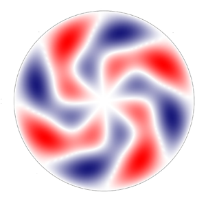
In figures 4 and 5, increasing $n$ causes the velocity profiles that are directly driven by the free stream forcing (2.1), i.e. $\bar {u}_r$, $\bar {u}_\theta$ and $\bar {u}_x^{(0)}$, to have a more intense modulation along the radial coordinate because the Bessel-function zeros $\xi _{mn}$, which appear in the argument of the Bessel functions in (2.1), increase in amplitude. The zeros $\xi _{mn}$ can thus be interpreted as analogous to wall-normal wavenumbers in the Cartesian geometry. Figures 4(c,d) and 6(c,d) show how the inner profiles (region II) and the outer profiles (region I) of the azimuthal velocities combine to create the composite profiles valid at any radial location. Figure 8 shows contour plots of the composite velocity components and the pressure at a fixed time instant in a cross-plane near the pipe mouth.

Figure 5.

Real parts of composite velocities $\bar {u}_x^{(0)}$, $\bar {u}_r^{(0)}$ in regions I and II for different $n$ values and $m=3$, $\bar {x}=0.018$, $Re_\lambda =4712$, $k_x=0.37$, $R=0.812$.

Figure 6.

Real parts of composite velocities $\bar {u}_x$, $\bar {u}_r$, $\bar {u}_\theta$ in regions I and II for different $m$ values and $n=2$, $\bar {x}=0.018$, $Re_\lambda =4712$, $k_x=0.37$, $R=0.812$.

Figure 7.

Real parts of composite velocities $\bar {u}_x^{(0)}$, $\bar {u}_r^{(0)}$ in regions I and II for different $m$ values and $n=2$, $\bar {x}=0.018$, $Re_\lambda =4712$, $k_x=0.37$, $R=0.812$.

Figure 8.

Contours of the instantaneous velocity components $2\bar {u}_{x,0},2\bar {u}_{r,0},2\bar {u}_{\theta,0}$ and pressure $2\bar {p}_0$ at $t=0$, $\bar {x}=0.018$, for $Re_\lambda =2356$, $k_x=0.185$, $R=0.6366$ ($n=3,m=4$).

The composite solutions (3.25)–(3.27) and (3.32) for $\bar {u}_x,\bar {u}_r,\bar {u}_x^{(0)}$ and $\bar {u}_r^{(0)}$ in regions I and II are used as initial conditions for the computation in regions V and VI.

3.2.2. Perturbation flow in regions III and IV

The outer expressions (3.22) do not take into account the viscous decay as they are only valid in the inviscid region I, i.e. for $\bar {x} \ll 1$. Viscous effects become important as the outer flow evolves downstream through region IV. The flow in regions III and IV can be found by a composite solution. The expression for the outer velocity field in region IV can be written as

(3.33)\begin{equation} \boldsymbol{u}= \left\{\frac{1}{r}\frac{\partial \psi}{\partial r}, -\frac{1}{r}\frac{\partial \psi}{\partial x} ,0 \right \} + \varepsilon \boldsymbol{u}_{out}\,\textrm{e}^{\textrm{i}(m \theta-k_x t)} + \text{c.c.}, \end{equation}

where the stream function $\psi (x,r)$ is given in (3.6) and (3.11). As depicted in figure 1, the base-flow pressure gradient only has a second-order effect through the $x$-dependence of $\psi (x,r)$. In the Cartesian geometry the outer velocity $\boldsymbol {u}_{out}$ can be obtained analytically by solving the parabolic region-IV momentum equation (5.9) on page 181 in Leib et al. (Reference Leib, Wundrow and Goldstein1999). In the cylindrical geometry, the radial and the azimuthal momentum equations are instead coupled and the system has to be solved numerically. The inner solution must also found numerically by solving the boundary-region equations (5.2)–(5.5) on page 180 of Leib et al. (Reference Leib, Wundrow and Goldstein1999), complemented by mixed-type boundary conditions obtained by asymptotically matching with the outer solution (3.33). These numerical calculations are not pursued herein because our region-V solution includes the solutions of regions III and IV and covers the whole streamwise flow evolution as the base-flow pressure gradient is accounted for at leading order.

4.1. Base flow

The base-flow streamwise and wall-normal velocity profiles across the pipe are shown in figure 9 at different streamwise positions. The small-$x$ asymptotic profiles (3.1) are also shown (dashed lines). The flow field approaches the fully developed regime as it develops downstream: the base-flow streamwise velocity evolves to the parabolic Poiseuille profile, while the wall-normal velocity decreases to zero.

Figure 9.

Streamwise (a) and wall-normal (b) base-flow velocity profiles. The solid lines denote the solutions at $x/(R^2 Re_\lambda )=0.0012$, 0.0036, 0.01, 0.03, 0.06, 0.12, 0.6 obtained by numerically solving the boundary-layer equations (2.8)–(2.9). The dashed lines show the composite solution of the streamwise velocity (3.12) (a) and of the wall-normal velocity (3.13) (b) at $x/(R^2 Re_\lambda )=0.0004$.

The base-flow streamwise velocity is shown in figure 10 at various $r/R$ locations as a function of the streamwise position. There is excellent agreement with the numerical data by Hornbeck (Reference Hornbeck1964) (red circles) and very good agreement with the experimental data by Reshotko (Reference Reshotko1958) (white circles), except at the two locations closest to the pipe wall, where the uncertainty of the measurements may have been influential.

Figure 10.

Base-flow streamwise velocity $\bar {U}$ at $r/R=0$, 0.2, 0.4, 0.6, 0.7, 0.8, 0.9 (from top to bottom) as a function of the streamwise coordinate, computed by numerically solving the boundary-layer equations (2.8)–(2.9) (solid lines). The symbols are experimental data by Reshotko (Reference Reshotko1958) (empty circles) and boundary-layer numerical data by Hornbeck (Reference Hornbeck1964) (red circles).

Figure 11.

Correction pressure function $\mathcal {K}$, defined in (4.1), as a function of the streamwise coordinate, computed by numerically solving the boundary-layer equations (2.8)–(2.9) (solid line). The symbols are numerical data by Sparrow et al. (Reference Sparrow, Lin and Lundgren1964) (red circles) and experimental data by Mohanty & Asthana (Reference Mohanty and Asthana1978) (white circles), Shapiro et al. (Reference Shapiro, Siegel and Kline1954) (square) and Knibbs (reported by Sparrow et al. (Reference Sparrow, Lin and Lundgren1964), triangle).

The downstream adjustment of the pressure gradient can be monitored through the correction pressure function

(4.1)\begin{equation} \mathcal{K}\left(\frac{x}{R^2 Re_\lambda}\right) = \frac{|\Delta \bar{P}^*|}{\rho^* U_\infty^{*2}} - \frac{8 \nu^* x^*}{R^{*2} U_\infty^*} = |\Delta \bar{P}| - \frac{8 x}{R^2 Re_\lambda}, \end{equation}

which measures the deviation of the base-flow pressure, defined in (2.5), from the fully developed Poiseuille value. Our numerical data, shown in figure 11, agree well with the numerical data based on the series solution by Sparrow et al. (Reference Sparrow, Lin and Lundgren1964) (red circles) and satisfactorily with the experimental data by Mohanty & Asthana (Reference Mohanty and Asthana1978). Our fully developed computed value, $\mathcal {K}_\infty =\lim _{x \rightarrow \infty }\mathcal {K}(x)=0.63$, matches the one by Sparrow et al. (Reference Sparrow, Lin and Lundgren1964) and is slightly lower than the experimental values by Shapiro, Siegel & Kline (Reference Shapiro, Siegel and Kline1954) (square) and Knibbs (reported by Sparrow et al. (Reference Sparrow, Lin and Lundgren1964), triangle).

We can define boundary-layer thicknesses to quantify the diffusion of the viscous effects as the flow develops downstream. They are defined as

(4.2)\begin{equation} \delta_k=\varDelta_k \int_0^R \left[1 - \frac{\bar{U}(x,r)}{\bar{U}_{cen}(x)}\right] \rm{d}r, \end{equation}

where $k=R$ identifies the boundary thickness that matches the pipe radius in the fully developed downstream limit ($\varDelta _R=3$ is obtained by substituting $\delta _R=R$, $\lim _{x \rightarrow \infty } \bar {U}(x,r)=2[1-(r/R)^2]$ and $\lim _{x \rightarrow \infty } \bar {U}_{cen}=2$ into (4.2)) and $k=LWG,PIPE$ denotes the boundary thickness that matches the one employed by Leib et al. (Reference Leib, Wundrow and Goldstein1999) as $x \rightarrow 0$, i.e., $\delta _{LWG}=(2 x/Re_\lambda )^{1/2}$ ($\varDelta _{LWG,PIPE}=\beta ^{-1} = 0.822$ is obtained by substituting (3.12) into (4.2)). Figure 12(a) shows the boundary-layer thicknesses as functions of the streamwise coordinate. The thickness $\delta _{LWG,PIPE}$ in our pipe-flow flow case is thinner than the corresponding Blasius-flow $\delta _{LWG}$ because of the accelerating core caused by the favourable pressure gradient.

Figure 12.

(a) Boundary-layer thicknesses $\delta _R$, $\delta _{LWG}$ and $\delta _{LWG,PIPE}$ as functions of the streamwise coordinate. (b) Second derivative of the streamwise velocity at the pipe axis and average error $\mathscr {E}$, defined in the text and measuring the deviation of the $\bar {U}$ profile from the Poiseuille solution, as functions of the streamwise coordinate.

We also quantify the entry length, i.e. the distance from the pipe mouth where region V ends and the fully developed region VI starts. The entry length is typically defined by the streamwise location where the axis base velocity $\bar {U}_{cen}$ reaches $99\,\%$ of its fully developed value. We can first use (23) in Durst et al. (Reference Durst, Ray, Ünsal and Bayoumi2005), i.e. $x_{e,u}=2 R[0.4642 +(2 C_{e,u} R Re_\lambda )^{1.6} ]^{1/1.6}$, where $C_{e,u}=0.0567$. As we operate under the assumption $Re_\lambda \gg 1$, Durst et al. (Reference Durst, Ray, Ünsal and Bayoumi2005)'s equation reduces to $x_{e,u}=4 C_{e,u} R^2 Re_\lambda$, which is consistent with the scaling adopted in figure 10. We compute $C_{e,u}=0.057$, which is within the uncertainty range provided by Durst et al. (Reference Durst, Ray, Ünsal and Bayoumi2005). We also quantify the entrance region as $x_{e,pres}=4 C_{e,pres} R^2 Re_\lambda$, i.e. the streamwise distance from the pipe mouth where $\mathcal {K}=0.99\mathcal {K}_\infty$, that is, where the pressure gradient has reached its fully developed constant value. We compute $C_{e,pres}=0.055$.

Crabtree, Küchemann & Sowerby on page 440 of Rosenhead (Reference Rosenhead1963) remark that in a pipe entrance flow: ‘… the whole of the fluid across a section becomes influenced by viscosity before the parabolic profile is reached’. We can examine this statement, although they do not specify how the diffusion of viscous effects is defined mathematically. The development of the flow to the Poiseuille parabolic profile is already quantified by the entry length $x_{e,u}$, based on the downstream evolution of $\bar {U}_{cen}$, but we also further monitor it by an adjustment length $x_{e,pois}=4 C_{e,pois} R^2 Re_\lambda$, defined as the streamwise location where the average difference between the streamwise velocity and the Poiseuille velocity, i.e. $\mathscr {E}(x)=R^{-1}\int _0^R |\bar {U}(x,r)-2[1-(r/R)^2]|\,\rm {d}r$ (shown by the dashed line in figure 12b), has decayed to 1 % of $\lim _{x\rightarrow 0}\mathscr {E}=2/3$. We find $C_{e,pois}=0.057$, i.e. the same as $C_{e,u}$. The diffusion of viscous effects can be quantified by two adjustment lengths. We first obtain $x_{e,u2}=4 C_{e,u2} R^2 Re_\lambda$, i.e. the downstream distance from the pipe mouth where the second derivative of the streamwise velocity with respect to the radial coordinate at the pipe axis, $\partial ^2\bar {U} / \partial r^2 |_{r=0}$ (shown by the solid line in figure 12b), is $99\,\%$ of its fully developed value. We choose this quantity because it represents radial viscous effects and the axis is the last radial location where the viscous diffusion from the wall is felt. We compute $C_{e,u2}=0.085$. We then find $x_{e,\delta }=4 C_{e,\delta } R^2 Re_\lambda$, i.e. the downstream distance from the entrance where $\delta _R=0.99$$R$, and obtain $C_{e,\delta }=0.059$. Table 1 summarizes the computed entrance lengths.

Table 1.

Entrance lengths according to the definitions in the text.

We therefore find that $C_{e,u2}$, $C_{e,\delta }>C_{e,u}, C_{e,pois}$, i.e. the flow becomes viscous for the whole wall-normal extent of the pipe slightly downstream from where the flow can be considered in good agreement with the Poiseuille profile. Therefore, there does not exist a distinct streamwise region along which viscous diffusion affects the whole wall-normal extent of the pipe and the velocity profile has not yet developed to the parabolic profile, which appears to be in contradiction with the statement by Crabtree, Küchemann & Sowerby. The adjustment length $x_{e,u2}$, based on the second wall-normal derivative of the streamwise velocity at the pipe axis, is the most conservative amongst the four lengths, as also visually evident in figure 12(b).

4.2. Perturbation flow

The downstream evolution of the perturbation flow is discussed in this section. The scaling adopted in § 2, which leads to $\boldsymbol {\bar {u}_{x,0}}=\boldsymbol {\bar {u}_{x,0}}(\bar {x},r;Re_\lambda, k_x, n,m,R,\hat u_x^\infty,\hat u_r^\infty )$, is useful for the asymptotic analysis and it relates directly to the open-boundary-layer case of Leib et al. (Reference Leib, Wundrow and Goldstein1999). However, it is does not convey an immediate physical meaning as, for example, the scaled frequency $k_x$ appears as an independent variable and in the scaling of $\bar {x}$. We therefore express the solution as $\boldsymbol {\bar {u}_{x,0}}=\boldsymbol {\bar {u}_{x,0}}(x_R,r_R;Re_R,\lambda _{xR},n,\lambda _R,\hat u_x^\infty,\hat u_r^\infty )$, where the subscript $R$ indicates scaling by the pipe radius $R^*$, i.e. $\lambda _R=\lambda ^*/R^*$. In the cylindrical geometry, varying the index $n$ allows studying the role of radial length scale, i.e. the larger $n$, the smaller the radial length scale.

In the analysis, we fix $\hat u_{x,mn}^\infty =1$, and the kinetic energy of the gust at the pipe mouth, defined as

(4.3)\begin{equation} \mathcal{E}_{gust,R} = \frac{\mathcal{E}_{gust}^*}{U_\infty^{*2} R^{*2}} = {\rm \pi}\int_0^1 ( |u_{g,x}|^2 + |u_{g,r}|^2 + |u_{g,\theta}|^2 ) r_R\, \mathrm{d}r_R, \end{equation}

(where $r_R=r^*/R^*$), is kept equal to $\mathcal {E}_{gust,11}$, the energy for $m=n=1$ and $\hat u^\infty _{r,11}=1$ ($u_{g,x},u_{g,r},u_{g,\theta }$ are the amplitudes of the free stream gust velocity components, defined in (2.1)). Expression (4.3) is written explicitly as

(4.4)\begin{equation} \mathcal{E}_{gust, R} = {\rm \pi}\int_0^1 \left[ r_R (\hat u^\infty_{x,mn} J_m(\bar{r}) )^2 + \frac{(4 \hat u^\infty_{r,mn} J_m(\bar{r}))^2}{r_R \xi_{mn}^2} + r_R \frac{( \hat u^\infty_{r,mn} J'_m(\bar{r}) )^2}{m^2} \right]\mathrm{d}r_R, \end{equation}

where $\bar {r}=\xi _{mn}r_R/2$ and $\hat u^\infty _{\theta,mn}$ has been eliminated by using (2.2). Setting $\mathcal {E}_{gust}=\mathcal {E}_{gust,11}$ allows computing $\hat u^\infty _{r,mn}$ for $m,n$ of choice and use of (2.2) gives $\hat u^\infty _{\theta,mn}$.

We first study the velocity and pressure profiles of a reference case that is representative of realistic water and air pipe-flow experiments. Table 2 presents the flow parameters of these cases. We then study the effect of the inflow parameters on the perturbation field.

Table 2.

Parameters for water and air pipe flow experiments. The unit Reynolds number is $Re_\infty ^*=U_\infty ^*/\nu ^*$ and $m=4$.

4.2.1. Initial reference-case flow

The region-I-II asymptotic initial conditions require a smooth matching with the numerical solutions of the boundary-region equations (2.11) and (2.12) at small $x_R$ locations. This matching is monitored by comparison in figure 13. The asymptotic profiles (dashed lines) are consistent with the numerical solutions (solid lines) at small $x_R$. The $\bar {u}_x$ profiles resemble the profiles of the Klebanoff modes appearing in free stream open boundary layers due to free stream vortical disturbances, shown in figure 3 on page 184 of Leib et al. (Reference Leib, Wundrow and Goldstein1999). This profile shape is expected because at short distances from the pipe entrance the flow confinement and the base pressure gradient do not play a leading role, a valid representation being given by the free stream boundary-layer region-II profile (3.25). Nevertheless, the amplitude and growth rate of $\bar {u}_x$ in our case are given by $\bar {u}_{\theta,com}$ in (3.23) and are thus influenced by the presence of the pipe wall. At these locations the dominant part of the total streamwise disturbance velocity $\bar {u}_{x,0}$ is due to $\bar {u}_x^{(0)}$, which is given in (3.27) and is caused by the direct free stream forcing action of the inviscid streamwise velocity in (3.19). The part due to $\bar {u}_x$ is smaller, which means that the streaks have not formed yet and do not dominate the boundary layers over the pipe wall.

Figure 13.

Streamwise and radial velocity components for the Reynolds number and the frequency of table 2 and $n=3$, $m=2$. The solid lines indicate the numerical solutions of the boundary-region equations (2.11) and (2.12) and the dashed lines indicate the asymptotic composite solutions used as initial conditions of the numerical calculations: (3.25) for $\bar {u}_x$; (3.27) for $\bar {u}_x^{(0)}$; (3.26) for $\bar {u}_r$; (3.32) for $\bar {u}_r^{(0)}$.

4.2.2. Downstream evolution of the reference-case flow

The downstream evolution of the disturbance field for the reference case of table 2 is investigated ($n=3,m=4$), assigned as perturbations at the pipe entrance. The inflow perturbations are streamwise-stretched vortices with comparable radial and azimuthal length scales in cross-sectional $r-\theta$ planes and a much longer streamwise wavelength. As discussed in § 2.3, at this bulk Reynolds number, $Re_R=1500$, no TS waves exist, but nevertheless an intense transient growth is detected. This growth is monitored by the energy of the perturbation, defined as

(4.5)\begin{equation} \mathcal{E}(x_R) = \underbrace{{\rm \pi} \int_0^1 |\bar{u}_{x,0}|^2 r_R \,\mathrm{d}r_R}_{\mathcal{E}_x} + \underbrace{{\rm \pi} \int_0^1 |\bar{u}_{r,0}|^2 r_R \,\mathrm{d}r_R}_{\mathcal{E}_r} + \underbrace{{\rm \pi} \int_0^1 |\bar{u}_{\theta,0}|^2 r_R \,\mathrm{d}r_R}_{\mathcal{E}_\theta}, \end{equation}

where $\bar {u}_{x,0}, \bar {u}_{r,0}, \bar {u}_{\theta,0}$ are defined in (2.7). Figure 14(a) shows that, while at the entrance the three velocity components have comparable intensity, the streamwise velocity component is the major contributor to the perturbation dynamics as the total energy increases from the pipe inlet, while the other two velocity components decay at comparable rate, as shown in the inset of figure 14(a). Downstream of $x_R=20$, the total energy is almost entirely due to $\bar {u}_{x,0}$. It reaches its peak at $x_R=28$ and then decays monotonically because of viscous dissipation. Almost no perturbation energy is computed downstream of $x_R=120$. The transient growth is confined to region V, upstream of the fully developed region VI, because the entry region, estimated through the centreline base velocity, terminates at $x_R=339$. The energy growth and decay is qualitatively similar the transient results in fully developed pipe flows by Reshotko & Tumin (Reference Reshotko and Tumin2001) in the spatial case and by O'Sullivan & Breuer (Reference O'Sullivan and Breuer1994) and Trefethen et al. (Reference Trefethen, Trefethen and Schmid1999) in the temporal case if the time scale is converted to the axial coordinate by use of the streamwise velocity at the pipe axis for qualitative comparison.

Figure 14.

(a) Streamwise evolution of the perturbation energy $\mathcal {E}$ and of its three parts $\mathcal {E}_x, \mathcal {E}_r, \mathcal {E}_\theta$ related to the velocity components. (b) Radial location of the maximum of $\mathcal {E}$ and amplitude of the wall perturbation pressure $p_w$ (inset).

As shown in figure 14(b), the maximum of the perturbation energy near the pipe mouth is confined near the pipe wall, within the base-flow viscous layer. As the flow evolves downstream, the perturbation spreads towards the core of the pipe, although its peak remains in the outer quarter radial region during the entire flow evolution (radial location $r_{\mathcal {E}}>0.6$). The inset of figure 14(b) depicts the downstream evolution of the magnitude of the pressure at the wall, i.e.

(4.6)\begin{equation} p_w(x_R) = |\bar{p}_0(r_R=1)| = \left.\frac{\lambda_R^3}{4 {\rm \pi}^2} \right\lvert \frac{\partial \bar{u}_{\theta,0}}{\partial r_R} + \left.\frac{\partial^2 \bar{u}_{\theta,0}}{\partial r_R^2} \right\lvert_{r_R=1}. \end{equation}

Relation (4.6) is obtained from the $\theta$-momentum equation (S2.8). The wall pressure decays up to $x_R=0.5$, grows to a maximum at $x_R=4$, and then decays monotonically downstream.

The radial profiles of $|\bar {u}_{x,0}|$ are shown in figure 15(a), for growing disturbances, and figure 15(b), for decaying disturbances. The base-flow streamwise gradients enhance the perturbation near the wall and the maximum of $|\bar {u}_{x,0}|$ moves towards the centreline at all streamwise locations. During the growth phase, the wall-shear stress induced by the perturbation remains constant, while it decays when the perturbation energy decreases.

Figure 15.

Profiles of the streamwise velocity amplitude $|\bar {u}_{x,0}|$ at different streamwise locations: (a) growing disturbance at $x_R=3.5$, 6.9, 13.7, 20.5; (b) decaying disturbances at $x_R=39.2$, 51, 62.9, 81.6.

The azimuthal velocity $|\bar {u}_{\theta,0}|$ in figure 16(a) decays at a faster rate near the centreline and so does the radial velocity $|\bar {u}_{r,0}|$ (not shown). Figure 16(b) confirms that the pressure $|\bar {p}_0|$ is closely related to $|\bar {u}_{\theta,0}|$ as the near-wall maximum of $|\bar {u}_{\theta,0}|$ is located at the same radial position of the local maximum of $|\bar {p}_0|$, although the overall maximum pressure disturbance is found at the pipe wall.

Figure 16.

Profiles of the azimuthal velocity amplitude $|\bar {u}_{\theta,0}|$ (a) and of the pressure amplitude $|\bar {p}_0|$ (b) at $x_R=8.7$, 13.7, 28.9, 45.9.

Figure 17 shows contour plots of the velocity components and pressure at a fixed time instant in a cross-plane where the total perturbation energy reaches its maximum. The spanwise and streamwise velocity components appear twisted about the pipe axis with respect to the initial symmetrical distribution observed near the pipe mount, shown in figure 8.

Figure 17.

Contours of the instantaneous velocity components $2\bar {u}_{x,0}$, $2\bar {u}_{r,0}$ and $2\bar {u}_{\theta,0}$, and the pressure $2\bar {p}_0$ at $t=0$, $x_R=28$, for $Re_R=1500$, $k_x=0.118$, $n=3$, $m=4$.

4.2.3. Effect of Reynolds number

Figure 18 shows the evolution of the total energy $\mathcal {E}$ at different bulk Reynolds numbers $Re_R$. As $Re_R$ increases up to approximately $Re_R=6000$, the perturbation energy increases, with the peak occurring farther downstream. The initial growth rate is independent of $Re_R$. For $6000< Re_R<10\,000$, the evolution of the energy up to the maximum is Reynolds number independent, while downstream of the peak the energy decays at a slower rate as $Re_R$ increases. This dependence on the Reynolds number also occurs in free stream boundary layers exposed to convected gusts, where the spanwise wavenumber $\kappa =k_z/\mathcal {F}^{1/2}$ is the governing parameter (Leib et al. Reference Leib, Wundrow and Goldstein1999). In figures 5 and 6 of Leib et al. (Reference Leib, Wundrow and Goldstein1999), as $\kappa$ decreases from 1 to 0.1 the the global perturbation energy, dominated by the streamwise velocity, increases and its maximum occurs farther downstream. This behaviour is thus consistent with figure 18, where $\kappa =m/(k_{x,R} Re_R)^{1/2}$ is in the range $0.12<\kappa <0.3$ for $1500< Re_R<10\,000$. The radial locations of the energy maxima move closer to the wall at larger $Re_R$ as the boundary layers becomes thinner (not shown).

Figure 18.

Effect of $Re_R$ on the downstream evolution of perturbation energy $\mathcal {E}$. The dashed line in this figure and in figures 19, 20 and 21 indicates the case of table 2 ($n=3, m=4$).

4.2.4. Effect of streamwise wavelength

Studying the influence of the streamwise wavelength $\lambda _{xR}$ of the oncoming disturbance is equivalent to studying that of the frequency because the two quantities are inversely proportional to each other and related through $U_\infty ^*$ for small-amplitude free stream gusts. Figure 19 shows that the initial amplitude of the perturbation energy is independent of $\lambda _{xR}$. Up to $x_R=10$, $\lambda _{xR}$ has no influence on the disturbance growth as the profiles overlap on one another. Farther downstream, longer wavelengths (i.e. smaller frequencies) lead to perturbations that grow more intensely, with their maxima occurring at larger $x_R$ locations.

Figure 19.

Effect of $\lambda _{xR}$ on the downstream evolution of total energy $\mathcal {E}$.

The trends at the two highest $\lambda _{xR}$ overlap (red line and thin black line), showing the independence of the dynamics in the limit of low frequency. The asymptotic scaling at large $\lambda _{xR}$ can be studied for $\epsilon = \mathcal {F} \ll 1$. In this limit, we introduce $\hat U = U$, $\hat V = \epsilon V$, $\hat x = \bar {x}/\epsilon$ and $\hat {u}_x = \bar {u}_x/\epsilon$. All the terms in the base-flow equations (2.8)–(2.9) are retained and the coefficient in front of the parenthesis in (2.9) changes to unity. The boundary-region equations (2.11)–(2.12) simplify as all the terms in (2.13)–(2.26) that are proportional to $i$, which are due to the unsteadiness of the oncoming disturbance (2.1), are asymptotically smaller, and $\mathcal {F}$ changes to unity. The low-frequency disturbance dynamics is thus steady at leading order. The analogous scaling for open free stream boundary layers was first found by Leib et al. (Reference Leib, Wundrow and Goldstein1999) on pages 183–185. In figure 19, the behaviour is consistent with the asymptotic analysis for $\epsilon \ll 1$: $Re_R$ is constant for those cases and thus it does not affect the scaling $\hat x$. At leading order the total energy is

(4.7)\begin{equation} \mathcal{E} \sim \frac{{\rm \pi} m^2}{k_x^2} \int_0^1 | \hat u_x |^2 r_R\, \mathrm{d}r_R = 4 {\rm \pi}^3 Re_R^2 \int_0^1 |\hat u_x |^2 r_R \,\mathrm{d}r_R, \end{equation}

which is independent of $\lambda _{xR}$. The prediction that the optimum conditions leading to the maximum transient growth are steady is fully consistent with the optimal-growth results of vortical perturbations that are present inside a Blasius boundary layer and evolve downstream from locations near the leading edge (Andersson et al. Reference Andersson, Berggren and Henningson1999; Luchini Reference Luchini2000). Figure 19 shows that oncoming perturbations with measurable unsteadiness, i.e. with frequency $f^*=1$ Hz ($\lambda _{xR}=200$) for the air pipe in table 2, are equally likely to lead to the flow breakdown as they achieve a growth which is very close to the optimal one.

4.2.5. Effect of radial characteristic scale

In the expansion based on Fourier–Bessel coefficients (2.1), the characteristic radial scale is defined by the zeros of the Bessel function $\xi _{mn}$. For fixed azimuthal index $m$, the larger the radial coefficient $n$, the smaller the radial length scale, as shown in figure 20(a) by the profiles of the real part of $\bar {u}_r$ at small $x_R$ locations. The transient growth decreases as the radial length scale of the free stream disturbance becomes smaller, as shown in figure 20(b). This effect is due to the more intense viscous dissipation caused by the large velocity gradients related to the small radial scale. The location of the maximum energy is computed closer to the pipe inlet as the radial scale decreases. For a Fourier–Bessel coefficient $n=9$, the perturbation decreases upstream of the expected transient growth and subsequent viscous dissipation. For $n=12$, the perturbation decreases at any streamwise location.

Figure 20.

(a) Real part of $\bar {u}_r$ for $m=4$ at $x_R=0.18$. (b) Effect of $n$ on the downstream evolution of total energy $\mathcal {E}$ for $m=4$.

The influence of the radial scale on the disturbance evolution cannot be investigated through the non-normality of the eigenfunctions of the developing boundary layers on the pipe wall. An eigenvalue-based approach would model the near-entrance disturbance as completely confined within the base-flow boundary layer, whereas the radial scale only pertains to the free stream gust flow and does not enter the classical stability problem of the boundary layer. The adopted boundary-region approach instead takes into account all the characteristics of the gust flow because, being an initial-value problem, the specification of the pipe-entrance flow is vital for the evolution of the perturbation inside the pipe.

4.2.6. Effect of azimuthal wavelength

Figure 21(a) shows the real part of $\bar {u}_\theta$ for $n=6$ near the pipe mouth, at $x_R=0.18$, for different $\lambda _{zR}=2{\rm \pi} /m$. For this $n$ value, varying $m$ only impacts on the azimuthal modulation of the disturbance, while the characteristic radial scale is maintained. The influence of the azimuthal wavelength $\lambda _{zR}$ on the perturbation energy inside the pipe is shown in figure 21(b). There exists an optimal $\lambda _{zR}$ (the reference $\lambda _{zR}=2.09$, $m=3$) that leads to the most energetic growth. This azimuthal coefficient was also found to lead to the most energetic spatial transient disturbance by Mayer & Reshotko (Reference Mayer and Reshotko1997) in a fully developed laminar flow. Disturbances with smaller $\lambda _{zR}$ are influenced by viscous dissipation that hampers their growth. Oncoming disturbances with a larger azimuthal wavelength, $\lambda _{zR}=3.14$ ($m=2$) are almost two-dimensional and do not lead to the maximum growth because the dynamics of the streaks is a strictly three-dimensional phenomenon (Leib et al. Reference Leib, Wundrow and Goldstein1999), unlike TS waves, the amplification of which is maximum in the two-dimensional case (Schmid & Henningson Reference Schmid and Henningson2001). The perturbations with $\lambda _{zR}=3.14$ persist downstream to larger distances than in the optimal case because they are less influenced by viscous dissipation due to azimuthal shear effects.

Figure 21.

(a) Real part of $\bar {w}$ for $n=6$ at $x_R=0.18$. (b) Effect of $\lambda _{zR}$ on the downstream evolution of total energy $\mathcal {E}$.

4.2.7. Comparison with experimental and numerical data

Wygnanski & Champagne (Reference Wygnanski and Champagne1973) experimentally studied the air flow in the entrance region of a circular pipe in order to understand the formation of turbulent slug and puffs. Just like Reynolds (Reference Reynolds1883), they recognized the impact of the entry disturbances on the flow character farther downstream, especially the intensity of inlet perturbations. They utilized an orifice, a suspended circular disk and a honeycomb to generate the perturbation at the pipe mouth. In the entrance region, i.e. where the flow is stable according to classical stability theory, Wygnanski & Champagne (Reference Wygnanski and Champagne1973) detected intense growth of low-frequency oscillations upstream of the turbulent region and proposed that ‘… the growth of perturbations is associated with the large shear existing within the boundary layer  …’. They also observed that the longitudinal fluctuations rose abruptly, much more than the cross-flow velocity components. These experimental results fully agree with our theoretical results.

Figure 22 shows their flow visualization of the pipe entrance flow by dye injection at two downstream locations. It is evident that, upstream of where the flow breaks down to turbulent puffs (right-hand part of figure 22a), the disturbances are elongated in the axial direction and characterized by a well-defined azimuthal length scale, as predicted by the low-frequency theory.

Figure 22.

Visualization of flow disturbances at $x_R=60$ (a) and $x_R=100$ (b) for an air flow in a pipe at $Re_R=1250$ (Wygnanski & Champagne Reference Wygnanski and Champagne1973). The arrows indicate the azimuthal wavelength in the developing regions. The flows are from the left to the right.

Figure 23 presents a comparison between our calculations and three sets of experimental data by Wygnanski & Champagne (Reference Wygnanski and Champagne1973). In figure 23(a,b), the base-flow comparison is excellent for the case at low level of free stream turbulence (figure 23a; $\vert u'\vert /\bar {U}_{cl}=0.16\,\%$, where $\bar {U}_{cl}$ is the centreline mean velocity), whereas the experimental base-flow data at much higher levels of free stream turbulence (figure 23b; $\vert u'\vert /\bar {U}_{cl}=5.8\,\%$, and $7.8\,\%$) deviate considerably from the base flow computed via (2.8) and (2.9). These results are expected because, when the oncoming disturbances are weak (generated by the upstream honeycomb), the nonlinear effects on the perturbation dynamics are negligible and do not distort the laminar base flow. When the disturbances are more intense (generated by the orifice and the suspended disk), nonlinearity distorts the base flow, even though the flow has not broken down to turbulence. The comparisons of the perturbation data, shown in figure 23(c,d), are consistent with the mean-flow results, i.e. much better agreement is obtained in the left graph, where nonlinear effects are likely to play a marginal role. The results in figure 23(c) are robust because the profile shape varies only slightly when the frequency, and the azimuthal and radial indexes, $m$ and $n$, are varied independently about the reference case $k_{x,R}=0.118$, $n=2$, $m=3$. The flow parameter ranges were chosen based on the description of the experimental conditions given in Wygnanski & Champagne (Reference Wygnanski and Champagne1973), i.e. streamwise wavelength longer than the radius and comparable azimuthal and radial length scales because generated by the honeycomb upstream of the pipe entrance. It would certainly be interesting to carry out further comparisons between better controlled experiments and computations of the nonlinear boundary-region equations and direct numerical simulations.

Figure 23.

Experimental data by Wygnanski & Champagne (Reference Wygnanski and Champagne1973) (symbols) and numerical profiles (solid lines) at $x_R=30$. (a,b) Base-flow streamwise velocity, computed by solving (2.8) and (2.9); (c,d) perturbation-flow streamwise velocity $\epsilon |\bar {u}_{x,0}|$ normalized by the maximum value, computed by solving (2.11) and (2.12); (a,c) $Re_R=9500$ and $\vert u'\vert /\bar {U}_{cl}=0.16\,\%$; (b,d) $Re_R = 1200$ and $\vert u'\vert /\bar {U}_{cl}=5.8\,\%$ (white circles) and $\vert u'\vert /\bar {U}_{cl}=7.8\,\%$ (black circles). Here $\bar {U}_{cl}$ denotes the centreline base-flow velocity. For all cases, the reference flow parameters are $k_{x,R}=0.118$, $n=2$, $m=3$.

Wu et al. (Reference Wu, Moin, Adrian and Baltzer2015) studied the pipe-flow entrance problem via direct numerical simulations. In one of their cases at $Re_R=4000$, the flow at the pipe inlet was a superposition of a uniform base flow and vortical disturbances located near the pipe wall with a quite distinct azimuthal modulation. The perturbation did not grow as the base flow evolved along the entry region and the breakdown to turbulence was detected much farther downstream, i.e. at locations where the laminar base flow reached the parabolic profile. This result qualitatively agrees with our theoretical prediction. A visual inspection of their figure 1D leads to an estimate of $m=8$ or larger, that is, sufficient for viscous effects to dominate and attenuate the algebraic growth, as observed in figure 21 ($m=8$ corresponds to $\lambda _{zR}=0.79$).