

1. Introduction
Orphan disease and their treatments are currently the focus of considerable policy attention. This policy attention arises because those who suffer from an orphan disease are perceived to be disadvantaged under the prevailing model of development for medical treatments, especially drugs. A number of factors inhibit the development of treatments for rare disease and access to those treatments that are developed. Orphan diseases are by definition rare (Wastfelt et al., Reference Wastfelt, Fadeel and Henter2006): in Europe, an orphan disease is defined as serious, life-threatening and affecting fewer than 1 in 2000 people (European Committee for Orphan Medicinal Products); Canada lacks an accepted definition, but the Canadian Organization for Rare Disorders (Canadian Organization for Rare Disorders) defines a rare disease as one affecting fewer than 1 person per 2000 people; and in the United States the Orphan Drug Act (1983) defined an orphan disease as one affecting fewer than 200,000 persons in the United StatesFootnote 1 or more than 200,000 persons with the expectation that drug development costs will not be recovered from sales (Dear et al., Reference Dear, Lilitkarntakul and Webb2006).
Since the orphan diseases are rare, the pharmaceutical industry has little financial incentive to develop new medicines for them. The small market size makes the return on investment insufficient to attract private capital. Treatments that are developed face a series of hurdles making it to the market and getting placed on insurance formularies. Clinical evidence of safety and efficacy is often less strong because of the small patient samples in randomized clinical studies and the reliance on surrogate markers of effectiveness that are not always well-linked to final outcomes (Drummond et al., Reference Drummond, Wilson, Kanavos, Ubel and Rovira2007b). The high fixed costs of development and the small number of patients lead to the high cost per patient (CP; DiMasi et al., Reference DiMasi, Hansen, Grabowski and Lasagna1991; Medecins Sans Frontieres, 2001). Consequently, the relatively high incremental cost-effectiveness ratios and the poor value for money frequently lead to denial of coverage (Drummond et al., Reference Drummond, Wilson, Kanavos, Ubel and Rovira2007a).
Several governments (e.g. United States, Japan and the European Union) have introduced special financial incentives such as tax credits to spur the development of treatments (‘orphan drugs’) for rare diseases (Cheung et al., Reference Cheung, Cohen and Illingworth2004; Dear et al., Reference Dear, Lilitkarntakul and Webb2006; Denis et al., Reference Denis, Simoens, Fostier, Mergaert and Cleemput2009).Footnote 2 Such incentives mitigate the industry's high risks and lower the potential return on investments in treatments for rare diseases. These incentive schemes have increased numbers of requests for the Orphan Designation of drugs by the US Food and Drug Administration and the European Medicines Agency (EMEA) (Denis et al., Reference Denis, Simoens, Fostier, Mergaert and Cleemput2009). However, such policies are of limited value if the treatments developed ultimately fail to get covered by insurers because of their high cost-effectiveness ratios. In response to this latter problem, some have proposed that funders apply a different, higher, cost-effectiveness threshold for drugs used to treat rare diseases (see, e.g. discussion in (Drummond et al., Reference Drummond, Wilson, Kanavos, Ubel and Rovira2007a)). This policy recommendation, however, is controversial.
Arguments for setting a higher cost-effectiveness threshold for orphan drugs vary, but the two most commonly invoked are rights-based arguments and the rule of rescue. Rights-based arguments posit that all members of society are entitled to access to a minimum amount of health care. Given this premise, rare disease sufferers have a right to a basic level of quality health care even if treatment does not offer the largest health gain for its cost (Hughes et al., Reference Hughes, Tunnage and Yeo2005). The rule of rescue principle asserts that society should come to the aid of those facing immediate, often life-threatening danger. In the orphan drug debate, the underlying premise of this principle is used to argue that society should not abandon the most severely ill individuals with rare diseases who need highly specialized treatment and have no other treatments available (Dolan and Olsen, Reference Dolan and Olsen2002; Hughes et al., Reference Hughes, Tunnage and Yeo2005).
Opponents of such a policy offer a corresponding set of arguments. Hughes et al. (Reference Hughes, Tunnage and Yeo2005), argue that orphan diseases are not inherently life-threatening, although many are debilitating and reduce life expectancy. McCabe et al. (Reference McCabe, Tsuchiya, Claxton and Raftery2006) characterize arguments based on the rule of rescue as emotional reactions to identifiable individuals in catastrophic events, but argue that unknown patients will become identifiable in the future, and hence it is an ethically invalid principle for policymaking. But perhaps the most common objection to setting higher cost-effectiveness thresholds for orphan drugs derives from the principle of maximizing the health gain achieved with society's limited health-care resources (Schlander, Reference Schlander2008). The opportunity cost of such a policy is larger health losses among those who suffer from common, highly prevalent diseases (Hughes et al., Reference Hughes, Tunnage and Yeo2005; Dear et al., Reference Dear, Lilitkarntakul and Webb2006; McCabe et al., Reference McCabe, Tsuchiya, Claxton and Raftery2006).
This debate has proceeded in a virtual vacuum of evidence regarding the views of the public regarding such a special status for drugs used to treat orphan diseases. We know that members of the public are, in general, willing to sacrifice a reduction in the total amount of health gain generated to achieve a more equitable distribution of health or health gains and to respond to those suffering severe ill-health (Nord, Reference Nord1993; Ubel et al., Reference Ubel, Spranca, Dekay, Hershey and Asch1998; Cookson and Dolan, Reference Cookson and Dolan1999; Dolan et al., Reference Dolan, Shaw, Tsuchiya and Williams2005). We do not know, however, if this holds for responding to the needs of those with rare diseases. The only direct evidence on this point offers partial support at best. The UK's Citizen's Council of the National Institute for Health and Clinical Excellence (NICE) recommended that the National Health Service pay higher prices for ultra-orphan drugs (affecting fewer than 1000 people in the United Kingdom) provided that in addition to being very rare, the disease is severe, life-threatening and there is evidence of health gain from treatment (NICE Citizens Council, 2004). Therefore, although rareness factors into their reasoning, rareness alone does not justify differential thresholds.
This paper presents the results of a pilot study that uses a discrete choice experiment to investigate individual preferences regarding public funding for drugs used to treat rare diseases. We view it as a pilot study because it is based on a convenience sample of individuals affiliated with a university. Since there is no universally accepted definition of an orphan disease or orphan drug, and the term carries strong normative overtones, we avoided use of the term ‘orphan drug’ in the experiment and instead focused on the underlying characteristics associated with orphan diseases. We explicitly include a condition's rarity and severity as attributes in our choice scenarios as these characteristics are often emphasized in defining orphan diseases. Further, the description of the context for the choice scenarios implies that there are no treatments available other than the drugs under consideration, as this feature also figures in debates about orphan drugs.
The study investigated three specific questions: (a) other things equal, are individuals willing to have the government pay more for drugs used to treat rare diseases than drugs used to treat common diseases; (b) other things equal, are individuals willing to have government pay more per life-year gained for a rare disease than for a common disease; and (c) in making recommendations regarding public coverage, do individuals place the same relative weights on attributes across rare and common diseases?
2. Methods
The study employs a discrete choice methodology (DCE) to investigate individual preferences for funding drugs. DCEs are based on the idea that people derive utility not from a good per se but from the underlying attributes of the good (Lancaster, Reference Lancaster1966). As such, a DCE presents respondents with a series of hypothetical choices that describe the choice alternatives by their underlying attributes and asks them which alternative they prefer. In our study, for instance, the attributes of the drug alternatives include the nature of the disease treated by a drug, a drug's effectiveness, and the cost of drug treatment (more on the attributes below). The values of the attributes vary across choice scenarios, and by observing the choices people make it is possible to infer their preferences over the attributes of the goods under study. DCEs are commonly used to identify people's preferences in a variety of non-market situations/services/commodities (Louviere et al., Reference Louviere, Hensher and Swait2000; Bateman et al., Reference Bateman, Carson, Day, Hanemann, Hanley, Hett, Jones, Loomes, Mourato, Ozdemiroglu, Pearce, Sugden and Swanson2002; Hensher et al., Reference Hensher, Rose and Greene2005) and have been widely utilized in health economics (Gerard et al., Reference Gerard, Shanahan and Louviere2003; King et al., Reference King, Hall, Lancsar, Fiebig, Hossain, Louviere, Reddel and Jenkins2007; Lancsar and Louviere, Reference Lancsar and Louviere2008; Ryan et al., Reference Ryan, Gerard and Amaya-Amaya2008).
2.1 Scenario for the discrete choice experiment
To put our experiment into context, respondents were told that specialised committees meet regularly to consider adding new drugs to public drug program formularies. However, the large number of potential drugs, the limited budgets and the high costs of such programs make public funding of prescription drugs a challenge. Participants were asked to imagine that they were a members of a government committee in the province of Ontario, Canada that makes decisions regarding drugs to be listed on the drug formulary for the province's public drug plan (see Appendix 1 for the exact description). They were told that the drug budget was limited and that there were more drugs available than could be funded within the budget; hence choices had to be made regarding which drugs to fund. They were then told that two drugs were being considered for listing on the formulary, presented with information on the two drugs and the conditions each drug is used to treat, and then asked which drug they would prefer to have the government fund under the public plan.
To reduce the chances that subjects might inject their own (erroneous) assumptions about the situation, the description explicitly stated that all patients were of similar age (mid-40s), marital status, income, education, etc. and could expect to live for 10 years without treatment. It was also noted that, if not treated, patients with both conditions consumed the same dollar amount of miscellaneous health care services in an effort to alleviate their symptoms. Finally, it was stated that the two drugs were identical in every respect except those characteristics explicitly described and that neither drug was associated with adverse side effects.
2.2 DCE attributes and attribute levels
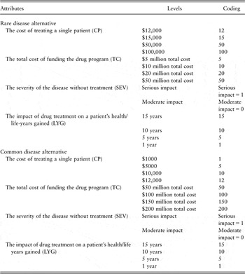
Potential attributes by which to describe the choice alternatives were identified by a review of the debate about coverage decisions for orphan drugs. This identified more potential attributes than could be included in the DCE. The full list of potential attributes was reduced based on two main criteria: importance in the debate about orphan drugs (judged subjectively by the frequency of mention and amount of attention given to the attribute) and the ability to specify the attribute in the DCE experiment. The attributes included in the scenarios were as follows (Table 1):Footnote 3
Attributes definitions and levels

• frequency of the disease;
• cost of treating a single patient with the drug;
• total cost of funding the drug (budget impact);
• severity of the disease without the treatment; and
• impact of drug treatment on a patient's health
Other attributes considered but not included in the final DCE (to keep the design manageable) were: the level of scientific evidence of clinical effectiveness for the drugs (orphan drugs often present lower grade clinical evidence compared to evidence for common diseases), the lack of available alternative treatments (orphan drugs might treat conditions that do not offer other therapies), and the cost-effectiveness ratios (orphan drugs often exhibit high incremental cost-effectiveness ratios and have poor value for money). The exact wording of the characteristics’ descriptions is provided in Appendix 2.
2.2.1 Frequency of the disease
Frequency of the disease treated by a drug is a primary attribute of interest. As noted, disease frequency was used as a label in the alternatives within each choice, and not as an explicit attribute. This allowed us to specify the other four attributes as alternative-specific and to test statistically whether respondents weigh the importance of an attribute differently across rare and common diseases. Frequency took on two levels: rare and common. Following the definitions of orphan diseases, we defined a rare disease as one with an incidence rate of less than 1 case per 2000 people; correspondingly, a common disease was defined as one with an incidence rate of more than 1 case per 2000 people. To aid understanding, the information was presented for a reference population of 10 million people (the approximate population of Ontario), with rare diseases having an annual incidence of fewer than 5000 cases and common diseases having an annual incidence of more than 5000 cases.
2.2.2 Cost of treating a single patient
Cost-per-patient was included as an indicator of the costliness of the drug treatment, and its inclusion allowed us to identify respondents’ views regarding the amount the government should be willing to pay at the margin for a drug treatment. To eliminate any potential confusion, the description emphasized that the full cost of treating a single patient occurred over a three-month period and that no other costs were incurred after this treatment period. Cost-per-patient took on seven levels ranging from $1000 to $100,000: three levels ($15,000, $50,000 and $100,000) occur only for rare disease alternatives, three levels ($1000, $5000 and $10,000) occur only for common disease alternatives, and one level ($12,000) occurs for both disease frequencies. The labeled design (described in more detail below) allows us to specify different levels for a given attribute across the two-labeled alternatives, in our case, rare and common diseases. Other things equal, we expected that subjects to prefer that government fund drugs with lower cost-per-patient.
2.2.3 Total cost of funding the drug program
Formulary committees commonly consider not only the cost-per-patient but also the total budget impact. This distinction can be particularly important for rare diseases, which can have a very high cost-per-patient but small budget impact because so few people have the disease. Total budget impact took on seven levels ranging from $5 million to $200 million: once again, three levels ($5 million, $10 million and $20 million) occur only for rare diseases, three levels ($150 million, $150 million and $200 million) occur only for common diseases, and one level ($50 million) occurs for both disease frequencies. Other things equal, we expected subjects to prefer that government fund drugs with lower total budget impact.
2.2.4 Severity of the disease without treatment
Severity of disease is consistently identified as a factor that individuals consider important for resource allocation in health care (Dolan and Olsen, Reference Dolan and Olsen2002). In the experiment, severity of disease if not treated could take on two values: serious and moderate impact. Severity was described in terms of the impact of the disease on a patient's quality of life and on the patient's self-assessed health status. The quality of life descriptions emphasized a patient's functioning with respect to their mobility, activities of daily living and pain levels, and were based on health state levels of the EQ-5D classification system corresponding to the mobility, usual activities and pain/discomfort (Dolan, Reference Dolan1997). ‘Serious’ severity corresponded to a self-assessed health rating of ‘poor’, while ‘moderate’ severity corresponded to a self-assessed health rating of ‘good’.Footnote 4 Although in some instances members of the public do not prioritize those who are severely ill (Dolan et al., Reference Dolan, Edlin and Tsuchiya2008; Donaldson et al., Reference Donaldson, Baker, Bateman, Jones-Lee, Lancsar, Loomes, Mason, Odejar, Prades, Robinson, Ryan, Shackley, Smith, Sugden and Wildman2008), other things equal, and considering that all drugs considered return patients to full health, we expected respondents to prefer that the government fund drug that treat those with a seriously severe condition rather than those with a moderately severe condition.
2.2.5 Impact of drug treatment on a patient's health
The last attribute was the health gain due to the drug treatment. The health gain was specified in terms of life-years gained as a result of treatment. This attribute took on four levels ranging from 1 to 15 life-years gained. In addition, respondents were told that, regardless of the baseline severity, each drug would return the patient to excellent health-related quality of life for their remaining lifetime. Other things equal, we expected respondents to prefer that the government funds drugs that produce a larger number of life-years gained.
2.2.6 Interactions among attributes
The design allowed for interactions among attributes. In choice experiments interaction effects are expected to account for a small portion of the variation (between 5% and 15% of the variance) and hence selected two-way interactions are normally sufficient (Hensher et al., Reference Hensher, Rose and Greene2005). The design accounted for three interactions: that between cost-per-patient and total cost, between cost-per-patient and severity and between severity and impact of treatment on health.
2.3 DCE design
2.3.1 Dependence among a subset of attributes
The design of the choice experiment was complicated by the fact that three of the attributes are linearly dependent. By definition, total budget impact (or total cost, TC) equals the product of the disease frequency (F) and cost-per-patient (CP): TC = F × CP. Hence, assigning values to two of them automatically determines the third. Yet we judged it important to specify explicit quantitative values for cost attributes rather than qualitative categories such as ‘high cost’ vs ‘low cost’ or ‘good value for money’ vs ‘poor value for money’. To resolve this problem, we varied independently the levels of the two cost attributes and left the disease frequency (incidence rates) to be the determined attribute that varied in the background within defined bounds consistent with a rare disease or a common disease. That is, the two cost attribute levels were chosen in such a way that the implied incidence rates were lower than 1 in 2000 cases for rare alternatives and greater than 1 in 2000 for common alternatives. For example, if the total cost is assumed to be $50 million, a cost-per-patient of less than $25,000 is consistent only with a common disease (a frequency of more than 5000, or an incidence rate of more than 1 in 2000 in a population of 10 million) and a cost-per-patient of $25,000 or more is consistent only with a rare disease (frequency of 5000 or less). Combinations of total cost and cost-per-patient correspond accordingly with incidence rates of less than 1 in 2000 people for a rare disease and greater than 1 in 2000 people for a common disease. Respondents never saw the implied incidence rates; they simply saw the labels ‘rare’ or ‘common’ disease.
We employed a labeled, forced-choice experimental design. Unlike generic experiments, labeled experiments brand each alternative, which subsequently carries information and meaning that are likely to influence the choice outcomes. Moreover, such designs allow for different sets of attribute levels across the alternatives. Hence, for every decision, respondents faced a choice between: a drug used to treat a rare disease with specified attribute levels for each of cost-per-patient, total budget impact, severity of disease and life-years gained by treatment; and a drug used to treat a common disease with correspondingly specified attribute levels.
Forced experiments constrain respondents to express a preference (i.e. make a trade-off among attributes) even when both alternatives are unattractive. Hensher et al. (Reference Hensher, Rose and Greene2005) argue that such a design is preferred when the objective of the study is to examine ‘the impact of the relationships different attribute levels have upon choice’ (p. 176), such as is the case in our setting.
2.4 Experimental design
A full factorial, labeled design with three four-level attributes and one two-level attributes generates 16,384 possible combinations (LMA = 42 × 3 × 22 = 16,384), and hence a fractional factorial design was used. Allowing for two-way interactions a D-efficient (D-efficiency = 0.817) fractional factorial design was produced with 64 pair-wise choices (Zwerina et al., Reference Zwerina, Huber and Kuhfeld1996; Kuhfeld, Reference Kuhfeld2005), which we blocked into 4 blocks of 16 choices each. All aspects of the experimental design were performed using SAS 9.1.3 built-in capabilities (Kuhfeld, Reference Kuhfeld2005).
2.5 Econometric methods
The utility an individual derives from choosing an alternative is assumed to comprise two components: a deterministic component and a stochastic component. Assuming an additive deterministic component to utility,  , and a stochastic component to utility, εiq, the utility of an individual q choosing alternative i is

where i denotes the choice alternative, k denote the attributes and q denotes an individual, and βk are the utility parameters to be estimated. βk are assumed to be homogeneous across the population.
2.5.1 Conditional logit vs latent class models
Assuming εiq to be independent and identically distributed (iid) extreme value type I (EV1), F(ε) = exp(−exp(−ε)) gives rise to McFadden's (Reference McFadden1974) conditional logit (CL), for which the probability that individual q chooses alternative i from among a set of J alternatives is:
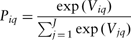
The CL model has a number of attractive features and is the standard approach to analyzing data from choice experiments, but it does impose some restrictive assumptions that often fail to hold (Hensher et al., Reference Hensher, Rose and Greene2005). In particular, its assumption of independence of irrelevant alternatives (IIA), its failure to incorporate preferences heterogeneity in the utility parameters and its inability to account for the panel structure of data have led researchers to identify models with more flexible structures. A commonly used alternative is the mixed logit model; and more recently, some have argued that the semi-parametric latent-class model (LCM) often performs as well or better than the mixed logit model (Greene and Hensher, Reference Greene and Hensher2003; Hole, Reference Hole2008).
In the LCM, parameter heterogeneity across individuals is modeled with a discrete distribution over a set of classes. ‘Individuals are implicitly sorted into a set of C classes, but which class contains any particular individual, whether known or not to that individual, is unknown to the analyst’ (Greene and Hensher, Reference Greene and Hensher2003: 682). The IIA is imposed only within classes and not on the observed unconditional probabilities. The probability that individual q chooses alternative i in choice set t conditional on falling within class c is
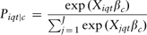
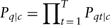
Following Greene and Hensher (Reference Greene and Hensher2003) let yqt denote a specific choice made such that Pqt |c = Prob(yqt = i|class = c). Hence, given a specific class assignment
In addition, let Hqc be the probability that individual q falls in class c
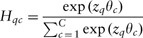
where zq is a set of variables that characterize the probabilities for class membership.
Following from equations (4) and (5), for c classes the likelihood for individual q is
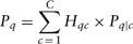
The number of latent classes is not determined endogenously but is determined a priori, based on the performance of alternative models with respect to information criteria such as the Akaike information criterion (AIC), the Bayesian information criterion (BIC) and the Hannan–Quinn information criterion (HQIC) (Hannan and Quinn, Reference Hannan and Quinn1979; Swait and Adamowicz, Reference Swait and Adamowicz2001; Hole, Reference Hole2008). We estimate and compare both CL and latent class models.
2.5.2 Variable specification
In addition to the choice attributes, our specification of Viqt includes three two-way interactions (TC × CP; CP × SEV; SEV × LYG) and information on cut-offs as described in Section 2.6. As explained below, such modifications allow for the relaxation of restrictive assumptions regarding the linearity of the attribute effects. Because of the labeled design, all attributes can be specified as generic or alternative-specific; a Wald test for the equality of attribute coefficients across rare and common alternatives can identify if alternative-specific attributes are appropriate.
We present results in three ways: the estimated model coefficients, marginal rates of substitution (MRS) among attributes (Bennett and Adamowicz, Reference Bennett and Adamowicz2001; with standard errors calculated using the delta method), and changes in the predicted probability of choosing a choice alternative caused by changes in the choice attributes. We are particularly interested in MRS between attributes and cost, which convey a marginal willingness to pay for an attribute. The marginal willingness to pay values are computed for changes evaluated at the means of the attributes; for the LCM, they are (along with the estimated coefficients) class specific. The changes in probabilities are computed for unitary changes at the mean of the regressors for total budget, cost-per-patient and life-years gained and for discrete changes for frequency and severity, while keeping the rest of the attributes to their sample mean values. All estimation and calculations were performed using Nlogit 4.0.
2.6 Allowing for discontinuities in marginal utility by incorporating decision cut-offs
By definition, discrete choice experiments are based on trades-offs between attributes. More of one attribute is assumed to compensate for less of another (Louviere et al., Reference Louviere, Hensher and Swait2000). However, in making choices individuals often employ decision heuristics that violate such compensatory behavior. Such heuristics can include, elimination-by-aspects (Tversky, Reference Tversky1972) and conjunctive rules (Dawes, Reference Dawes1964) in which subjects follow cut-offs when making choices. A cut-off is a decision rule that sets limits beyond which the subject would never choose an alternative (e.g. a ‘rule’ that one would never buy a house without a swimming pool or they would never pay more than $X for a specific product). However, even when individual use such cut-off rules, the evidence shows that they often do not follow them strictly (Huber and Klein, Reference Huber and Klein1991; Swait, Reference Swait2001). In a sense, rather use hard cut-offs individuals seem to employ as soft cut-offs, or thresholds, around which the marginal utility of an attribute level varies. This possibility is important because standard discrete-choice experiments assume no such discontinuities in the marginal utility of attributes.
The difficult nature of the decision problems we presented subjects regarding drug coverage suggested to us that they might employ non-compensatory decision heuristics. We therefore included in our study a component that would enable us to test for discontinuous utility with respect to attributes. In implementing this we followed Swait (Reference Swait2001), who proposed a penalizing utility function that allows for cut-off violation and approximates/simulates a number of non-compensatory behaviors. In this framework, decision cut-offs are not ‘hard’ in the sense that a person never violates them; rather, it assumes that subjects suffer a greater loss in utility at the margin the further one is from the threshold (i.e. there is a utility penalty for such a choice).
Implementing this approach required that we collect, for each attribute in the study, information on the value of each respondent's cut-offs (below or above which they would ‘never’ choose an alternative). For example, if a subject agreed that ‘the government should not fund drug treatments that extend life fewer than 5 years’, this would provide information regarding the lower cut-off (or threshold) the subject placed on the attribute life-years gained.
Following Swait (Reference Swait2001), for choice i and k attributes, allowing for cut-offs modifies the deterministic component of equation (1), as follows

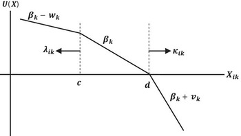
where ck and dk are the lower and upper cut-offs as stated by the respondent, max(0, ck − Xik) identifies the magnitude of the violation of the lower bound cut-off and max(0, Xik − dk) identifies the corresponding violation for the upper bound cut-off. For an attribute with a negative marginal utility (e.g. cost), let the initial negative slope be βk (see Figure 1). If a subject were to choose an alternative with a cost over a specific upper threshold ‘d’, marginal utility falls at a higher rate (βk + vk); if they choose an alternative with cost below ‘c’, marginal utility falls at a lower rate (βk + wk). Marginal utility displays kinks, where ‘c’ and ‘d’ are the lower and upper cut-offs. Our specification does not include both upper and lower thresholds for an attribute, but it does include upper cut-offs for some attributes and a lower cut-off for others, and therefore equation (7) above includes two indicator variables, λk and τk, where λk takes on a value of 1, if the attribute is hypothesized to have a lower cut-off and 0 otherwise, and τk takes on value of 1 if the attribute is hypothesized to have an upper cut-off and 0 otherwise.
The impact of cut-off violation on a negatively sloped attribute (e.g. cost) (from Swait, Reference Swait2001: 912).

As Swait (Reference Swait2001) further shows, cut-off violation is possible even for binary indicators, where a violation becomes itself a dummy variable indicating a case where the level of the attribute differs from that stated in the cut-off elicitation exercise. The subjects completed the cut-off elicitation questions before completing the choice experiment. The elicitation method involved asking subjects a series of questions formulated, such as “I would never pay more than $X to fund this drug” (see Appendix 3).
The cut-off information is integrated into the analysis by including in the regression the second and third terms of equation (1), with their coefficients estimated along with the rest of the parameters. The magnitude and statistical significance of the associated coefficient estimates provide a test of the importance of discontinuities in the subjects’ decisions (compared to a model that assumes cut-offs are not present) (Danielis and Marcucci, Reference Danielis and Marcucci2007). Non-significant coefficients on the cut-off variables imply that such cut-off values play no role in decision-making.
2.7 Survey development and administration
Development of the survey instrument was refined by two pre-tests. The first pre-test was conducted among a convenience sample of colleagues, research staff and graduate students early in the development of the instrument. This pre-test focused on basic aspects of the survey design such as the instructions, design of the choice scenario and specification of the attributes. The second pre-test was conducted among a sample of 50 individuals drawn from the subject pool and focused on final refinement of the survey, clarity and understanding by respondents and testing the procedures for administering the survey. As part of this pre-test, respondents also completed open-ended questions regarding the clarity and difficulty of the content and length of time required to complete the survey. In addition, five in-depth interviews with a random sample of pre-test subjects provided further insight into points of ambiguity or other problems. Revisions were made in light of the feedback.
For the main survey, a random sample of individuals was drawn from a subject database maintained by the McMaster University Experimental Economics Laboratory and invited to participate in the study. Following recommendations on sample size (Hensher et al., Reference Hensher, Rose and Greene2005; Lancsar and Louviere, Reference Lancsar and Louviere2008), 20 to 50 participants per block was deemed adequate for robust estimation, suggesting a target sample of 200 individuals. The vast majority of subjects were students. Past experimental valuation studies (Maguire et al., Reference Maguire, Taylor and Gurmu2003; Depositario et al., Reference Depositario, Nayga, Wu and Laude2009) have concluded that the views of students often closely represent those of the broader community of non-students. However, given the use of a convenience sample of individuals from the university, we view this study as a pilot that can produce initial evidence and inform the design of subsequent studies in the general community. All participants were compensated $8 for their participation.
The full survey was administered electronically in the McMaster University Experimental Economics Laboratory. Ethics approval for the study was obtained from the Hamilton Health Sciences/McMaster University Research Ethics Board.
3. Results
3.1 Sample descriptive statistics
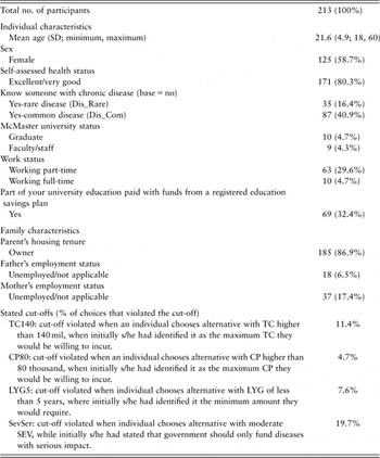
A total of 213 respondents completed the survey. The sample characteristics are as follows (Table 2): 59% were female; mean age was approximately 22 years; 80% reported excellent or very good health status; about 30% had a part-time job; for 6.5% and 17.4% the father or the mother, respectively, was unemployed; for approximately 87%, their parents owned their house; and 32% financed their education at least partly through a registered education savings plan (RESP), which is generally used by those with above-average income.
Sample descriptive statistics

CP = cost-per-patient; TC = total cost; LYG = life-years gained; SEV = severity.
3.2 Multivariate results
3.2.1 Model selection
Information criteria (AIC, BIC and HQIC) indicated that did the two-class LCM performed better than the traditional CLFootnote 5 (CL: AIC = 1.026, BIC = 1.048, HQIC = 1.033; LCM: AIC = 0.97, BIC = 1.047, HQIC = 1.003). Within the LCM, specifying more than two classes often resulted in convergence problems and singularities in the variance matrices. However, in cases in which convergence was achieved, the specification with two classes was preferred to the specification with more than two classes. A test of the joint statistical significance of the alternative-specific attributes indicated that a generic model was preferred (χ 2 = 15.058; p-value = 0.37). We therefore present results from the two-class LCM with generic attribute coefficients. Finally, an LR test (χ 2 = 51.1; p-value = 0.000) implied the joint significance of the cut-offs and, hence they were kept in the model.
3.2.2 Coefficient estimates
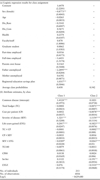
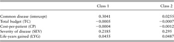
Table 3(a) presents the results of the logit model regarding the probability that each individual falls into each of the two latent classes, with the assignment being based on a set of personal characteristics. Among the characteristics included in the model only sex, father's employment status and whether the respondent's university education is at least partly financed by a RESP are statistically significant predictors of class membership. The table presents the logit coefficients, and therefore the results imply that the odds that a female is in class 1 are 0.42 times those of a male; the odds that a subject whose father is unemployed is in class 1 are 0.08 those of a person whose father is employed; and the odds that a subject who finances their education at least partly through an RESP is in class 1 are 2.81 times those who do not.Footnote 6 The two classes are of approximately equal size with the average probability that a respondent falls into class 1 being 46% and the average probability for class 2 being 54%.
Latent class model results (two classes)

CP = cost-per-patient; TC = total cost; LYG = life-years gained; SEV = severity.
Standard errors in parentheses; *significant at 10%; **significant at 5%; ***significant at 1%.
Table 3(b) presents the attribute coefficients for each class. We discuss the estimates separately for each class and then compare them. For class 1, the significant common disease intercept indicates that, all else equal, respondents preferred that the government fund drugs for common diseases. The coefficients on both total budget impact and cost-per-patient are not statistically significant for either common or rare diseases, implying that neither cost attribute influenced preferences over funding for a drug. Neither are the interaction terms involving these two cost attributes (TC × CP and CP × SEV) statistically significant. The coefficients for baseline disease severity and for life-years gained by treatment are significant and positive. As expected, respondents prefer that government fund a drug to treat a serious condition rather than a condition of moderate severity, and that it fund a drug that produces more life-years gained. Table 4 presents the impact of a one-unit change (or discrete change) in each attribute on the probability that subjects prefer funding a drug. The change from rare to common disease increases this probability by about 30 percentage points, while the corresponding effect for the two cost attributes is not statistically different from zero. For SEV, the probability that a subject prefers to have government fund a drug used to treat severe a condition was 22 percentage points higher than for a moderate condition. For life-years gained by treatment, an increase of one life-years gained increases by 4.5 percentage points the probability that a subject prefers to have government fund a drug.
Change in the probability of choosing a drug associated with a one-unit change in an attribute

Note: Changes are computed for unitary changes at the mean for TC, CP, LYG and for discrete changes for frequency and SEV, while keeping the other attributes at their sample mean.
For class 2, though the trend again favours a common disease, the common disease intercept is smaller and not statistically significant, indicating that the frequency of disease exerted little influence on subject choices. The coefficient estimates on both TC and CP are negative and statistically significant. It appears, therefore, that for class 2 costs influence choice in the expected direction (greater cost reduces the probability of funding a drug). The coefficient on the interaction term TC × CP is statistically significant and possesses an unexpected positive sign. However, the aggregate effect (TC + CP + TC × CP) is negative over the values of CP and TC that appear in our design.Footnote 7 The implied magnitudes of these cost effects are as follows: a $1 million increase in the total budget impact is predicted to decrease the probability that a drug is chosen by a 0.07 percentage point; for cost-per-patient, a $1000 increase in cost-per-patient is predicted to decrease the probability that a drug is chosen by 0.12 percentage points. As we saw for class 1, the coefficient estimates for both baseline severity of illness and life-years gained are positive and statistically significant, and the estimates again imply large effects on choice. The probability that a drug is chosen for government funding is 29.5 percentage points higher if it is used to treat a severe condition than if it is used to treat a moderate condition. In addition, an increase in 1 life-year gained raises the probability that a drug is chosen for government funding by 4.9 percentage points. The interactions term CP × SEV has an unexpected positive sign, implying that for cases involving a serious disease an increase in CP makes the alternative more attractive. As expected, the interaction effect is positive for severity and life years (SEV × LYG).
The coefficient estimates associated with the cut-off analysis are presented at the bottom of Table 3. None of the estimates approach statistical significance for class 1, while for class 2 there is evidence of discontinuity with respect to two attributes: disease severity and life-years gained by treatment. Hence, for those in the sample who stated an a priori intention to not fund anything with moderate severity but subsequently violated it, the estimate implies that the ‘penalty’ is −0.191 ‘utils’: the coefficient for choosing a moderate condition is 0 (i.e. baseline of a binary indicator), and hence, the penalty is 0+(−0.191)). Similarly, for those stating an intention to not fund anything that extended life less than five years, choosing a drug that generates fewer than five additional life years has a negative impact on utility. The magnitude of the penalty is larger than that effect of the attribute itself and implies that for drugs that produce fewer than five additional life years, the utility obtained from life years is negative (0.1823 − 0.5335 = −0.3512).
3.2.3 Marginal rates of substitution
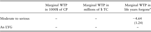
Tables 5 and 6 present MRS among selected attributes. The calculated MRS are meaningful only when both attribute coefficients are statistically significant. Hence, for class 1 (Table 5), we present MRS only with respect to severity and life-years gained by treatment. On average, individuals of class 1 are willing to forgo 4.6 life years to fund a drug that treats a serious condition rather than a moderate one. This implies that individuals are equally willing to have government fund a drug that treats a serious condition as a drug that treats a moderate condition and produces an additional 4.6 life-years gained for recipients.
Marginal rates of substitution in monetary and life years for Class 1
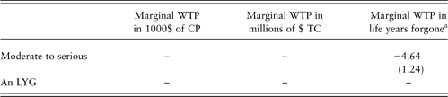
WTP = willingness to pay; CP = cost-per-patient; TC = total cost; LYG = life-years gained; SEV = severity.
Standard errors in parentheses computed through the delta method.
aWTP calculations are computed at the mean of the attributes, that is, for the figure in the table we would have  .
Marginal rates of substitution in monetary and life years for Class 2
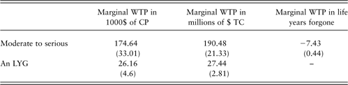
WTP = willingness to pay; CP = cost-per-patient; TC = total cost; LYG = life-years gained.
Standard errors in parentheses computed through the delta method.
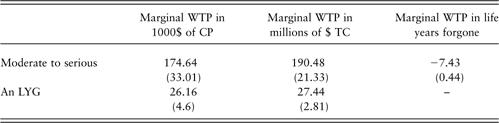
Individuals in the second class (Table 6) are willing to forgo slightly more life-years gained (7.4) to treat a serious condition rather than a moderate one. The significance of the cost attributes in class 2 allows for the calculation of monetary marginal willingness to pay (WTP). Individuals are willing to have government spend an extra $174,640 per patient to fund a drug used to treat a serious condition compared to a drug used to treat a moderate condition. They are willing to have government incur an additional total cost of $190 million to treat a serious condition rather than a moderate one.
Finally, all else equal, individuals are willing to have the government spend an additional $26,160 cost-per-patient for an extra life-year gained by treatment and an additional $27.44 million in total to fund a drug that provides an extra life year gained for all those who receive treatment.
4 Discussion
This exploratory study is a first attempt to present empirical evidence regarding individual preferences about funding for drugs used to treat orphan diseases. The frequency of a disease in a population is only one feature of a disease relevant to funding coverage decisions, making DCE well suited to investigating how and to what extent disease frequency influences people's judgments regarding public funding for a drug.
Our study was designed to answer three specific questions with regard to coverage decisions: (a) other things equal, are individuals willing to have the government pay more for drugs used to treat rare diseases than drugs used to treat common diseases; (b) other things equal, are individuals willing to have government pay more per life-year gained for a rare disease than for a common disease; and (c) in making recommendations regarding public coverage, do individual place the same relative weights on attributes across rare and common diseases.
Our results indicate that the answer to the first question is no: other things equal, a subset of people (class 1) actually appear willing to have government pay less for drugs used to treat rare diseases; however, another subset (class 2) makes no distinction based on frequency of disease.
For the second question our results indicate the answer to be also no: people do not appear willing to pay more per life-year gained for those who suffer from a rare disease than those who suffer from a common disease. Statistical tests rejected the alternative-specific models in favor of a single generic specification, which implies that individuals do not weigh attributes differently across common and rare diseases when making funding decisions. Our results, however, do indicate heterogeneous preferences between the two latent classes. For those who fall in latent class 1, costs do not exert a meaningful influence on choice; for those who fall in latent class 2 and for whom costs do exert an important influence on decisions, the willingness-to-pay for an additional life-year gained by treatment did not differ between common and rare diseases.
Finally, the results indicate that the answer to the third question is no: respondents did not weight attributes in a meaningfully different way across common and rare diseases. The Wald test could not reject the null hypothesis of no difference, so that coefficient estimates are not statistically different from each other.
We do find large effects for those attributes that the literature on priority-setting suggests we should: severity of disease and treatment effectiveness. For both latent classes, the influence of these two attributes outweighs all other influences. These findings are also consistent with the findings of NICE's Citizens Council – the only other evidence currently available regarding the public's views on coverage for drugs used to treat orphan diseases – that rareness itself does not justify special consideration, but rather that severity, established evidence of effectiveness and the life-threatening character of the disease weighed more heavily (NICE Citizens Council, 2004). Our findings regarding the lack of emphasis on costs for those in class 1 are consistent with a Canadian study that used a citizen jury to investigate public views on criteria for priority-setting for health technology assessment. Members of the citizen jury argued that cost should not be considered during priority-setting for HTA but that high incidence, quality of life and potential to extend life should be among the top criteria (Menon and Stafinski, Reference Menon and Stafinski2008). In particular, ‘of greatest importance was the “potential to benefit a number of people” reflecting the jury's view that technologies for highly incident/prevalent conditions within a population should be given higher priority over less prevalent ones’.
The differences in choice behavior across the two classes may reflect the broader divisions in the debate about coverage decision-making. There is no such thing as a single ‘view’; rather, there is systematic heterogeneity that the LCM was able to identify. Specifically, one approach to coverage decision-making (Class 1) put little weight on cost considerations, focusing almost exclusively on severity and treatment effect; in contrast, the second (Class 2) considered costs in addition to severity and treatment effect. Note that an individual's class cannot be identified (i.e. latent) but overall, across the whole sample, the two tendencies are almost of equal frequency. Hence, in debates about coverage decision-making, one would expect differing positions, one of which emphasizes the importance of considering costs and the other of downplays such considerations. Interestingly, our results also suggest that the decisions of males and those of higher socio-economic status (father employed and finances education through registered savings accounts) have a stronger tendency to downplay considerations of costs. The ability to accommodate such heterogeneity is a strength of the LCM and the likely reason why both in this and previous studies (Greene and Hensher, Reference Greene and Hensher2003; Hole, Reference Hole2008) it performed better than the more commonly applied CL model.
Our results find some evidence of discontinuity for two attributes in Class 2, indicating that the marginal utilities of SEV and LYG are not constant over the whole range of values presented. However, the forced-choice nature of our design may have compromised our ability to accurately identify such effects and exaggerated their presence. For instance, an individual may have faced two alternatives, both of which violated a decision cut-off (e.g. life-years gained for each alternative was below the respondent's self-declared cut-off), but still was forced to choose one as the preferred alternative. Even with such potential exaggeration, raw averages present little evidence of cut-off violation (Table 2). It should be noted that our main results are not sensitive to the inclusion or exclusion of the cut-off variables from the model.
The assumption that treatment restored individuals to full health resulted in some loss of realism for the choice scenario, but was made for two primary reasons. First, it created a cognitively simpler choice task for the respondents. Pre-testing revealed that explicitly varying baseline severity, number of life-years gained and post-treatment quality of life were cognitively much more difficult to evaluate. Second, including a separate attribute for post-treatment quality of life would create saliency problems and would require imposing design restrictions with respect to severity. For example, a drug used to treat a severe disease that resulted in a higher quality of life than a drug used to treat a moderate disease could potentially raise questions about the effectiveness of the drugs, which was outside the scope of this study.
Further, our statement in the scenario description that all patients were of a similar age (mid-40s) was included to ensure that respondents used the same reference point for all alternatives when making choices. There is evidence that individual preferences regarding health can vary with the age of the patient (Dolan et al., Reference Dolan, Shaw, Tsuchiya and Williams2005), which it potentially limits the generalizability of our results to patient populations of a different age.
Overall, our results indicate that the participants (in this case, represented by a university-affiliated sample from Ontario, Canada) do not support differential consideration of orphan diseases for coverage decision-making. They therefore send a cautionary message about implementing special coverage rules for drugs to treat orphan diseases. Two considerations, however, should determine the role of this evidence in the debate. First, even assuming that we have accurately elicited the views of the public, such preferences are not necessarily determinative in resolving difficult ethical problems such as funding treatments for orphan diseases. The resolution of such issues normally requires consideration of both sound ethical reasoning from principles and the preferences and attitudes of members of society. Second, as the first empirical results on this question, these findings should be seen as tentative and subject to further research both in different populations (i.e. generalizability of student samples is hard to advocate) and using modified designs (i.e. more comprehensive utility functions e.g. degree of rareness) to validate any conclusions. Although it is reasonable to observe differences in views across populations, such research can help identify potential framing effects associated with any single study and those aspects of the results that are robust across studies.
Acknowledgments
We, the authors are grateful to two anonymous reviewers for their valuable suggestions. In addition, we would like to thank Mita Giacomini and Jean-Eric Tarride for helpful comments and advice. We thank colleagues in the NET group at McMaster University for useful feedback regarding the design of the experiment and the analysis of the data, and we thank David Cameron and Aleksandra Gajic for assistance administering the survey. This research was funded by the Canadian Institutes of Health Research (Grant no. 76670). We also acknowledge funding from the Ontario Ministry of Health and Long-term Care to the Centre for Health Economics and Policy Analysis, McMaster University. The views expressed are those of the authors alone.
Appendix 1
Exact description and wording of discrete choice experiment exercise
In this part of the questionnaire, we are interested in your preferences with respect to funding drugs. Each scenario will present information about two health conditions, a drug used to treat each of them, the effect of each drug on a patient's health, and the cost of each drug. For each scenario you will be asked to choose which drug you would prefer that the government include within its public drug plan. If a drug is funded by the public plan patients with the condition can obtain the drug free of charge. The two drugs, the diseases they treat, and the individuals who suffer from the diseases differ only with respect to the attributes listed in the scenario. All other aspects of the decision problem should be assumed identical across the two choice options.
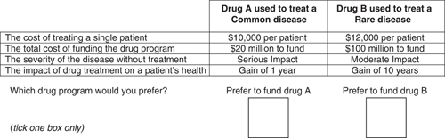
Example scenario
Imagine that you are a health-care decision maker on an Ontario government committee that has been asked to decide which of the two drugs will be included within the public drug insurance program. Both drugs are used to treat conditions that arise in the general population. When answering the question below, assume that the characteristics of patients who develop the respective diseases are identical in all respects (e.g. age, marital status, income, education, etc.) except those explicitly mentioned. The two drugs are also identical except with respect to attributes described below; neither drug is associated with adverse side effects. The money used to fund the chosen drug will come from the provincial public health-care budget, which in 2008 was $46 billion. Only one drug can be funded. Please indicate whether you prefer to fund drug A or drug B by placing a tick on one of the boxes below. There are no right or wrong answers.
Example choice problem:
Appendix 2
Exact wording of the five characteristics’ descriptions
– The frequency of the disease in the population
This attribute indicates how often the disease occurs in the population. This can take on two values:
Rare disease: the disease is rare, with less than one case occurring each year for each 2000 people in the population. In a population of 10 million people (the approximate population of Ontario), fewer than 5000 cases would occur each year.
Common disease: the disease is common, with more than one case occurring each year for each 2000 people in the population. In a population of 10 million people (again, the approximate population of Ontario), more than 5,000 cases would occur each year.
– The cost of treating a single patient
This attribute indicates the total one-time treatment cost for a single patient. All treatment costs arise during a three-month treatment period; no additional treatment costs occur once this is completed. There are seven possible cost values:
• $1,000
• $5,000
• $10,000
• $12,000
• $15,000
• $50,000
• $100,000
– The total cost of funding the drug program
This attribute indicates the total annual cost to the Ministry of Health if the drug program is funded publicly. There are seven possible costs should a drug be funded by the public plan:
• $5 million total cost
• $10 million total cost
• $20 million total cost
• $50 million total cost
• $100 million total cost
• $150 million total cost
• $200 million total cost
– The severity of the disease without treatment
This attribute indicates the seriousness of a disease if the patient does not obtain treatment. All the diseases you will be asked to consider strike people in their mid-40 s. In all cases, once diagnosed, patients who do not receive treatment die prematurely; without treatment, they can expect to live 10 years following diagnosis. Each disease also affects a person's quality of life. The impact on quality of life can take on two values (even after taking into account the effect of miscellaneous services patients seek in an effort to relieve symptoms):
Serious Impact: Patients who suffer from this disease have trouble with their mobility, need help with daily activities and suffer from strong pain. Overall, when asked to rate their health as excellent, good, fair or poor, most patients with the disease rate their health as poor.
Moderate Impact: Patients do not have trouble with their mobility or daily activities, but suffer from minor pain, discomfort, and need rest until their complaints disappear. Overall, when asked to rate their health, most patients with the disease rate their health as good.
Note: Regardless of whether the impact is serious or moderate, patients who are not treated with a drug consume the identical dollar value of miscellaneous health care services in an effort to alleviate their symptoms.
– The impact of drug treatment on a patient's health
The drug treatment improves both quality of life and expected length of life. In all cases, the drug returns recipients to excellent health-related quality of life while alive. The impact of the drug treatment on life expectancy takes on four possible values:
• Patients treated with the drug expect to live 15 years longer than those with the disease who do not receive treatment. That is, rather than live only 10 years after diagnosis, a patient treated with the drug can expect to live 25 years.
• Patients treated with the drug can expect to live 10 years longer than those with the disease who do not receive treatment. That is, rather than live only 10 years after diagnosis, a patient treated with the drug can expect to live 20 years.
• Patients treated with the drug can expect to live 5 years longer than those with the disease who do not receive treatment. That is, rather than live only 10 years after diagnosis, a patient treated with the drug can expect to live 15 years.
• Patients treated with the drug can expect to live 1 year longer than those with the disease who do not receive treatment. That is, rather than live only 10 years after diagnosis, a patient treated with the drug can expect to live 11 years.
Appendix 3
In this part of the questionnaire we ask you to indicate your agreement or disagreement with each of a series of statements listed below. Please read each statement carefully before responding, as differences between some statements are small but important. For each statement, please indicate whether you agree or disagree by placing a tick in the appropriate box.