3.1. The SGS kinetic energy equation

Since the $k$-equation model was proposed by Schumann (Reference Schumann1975) and Yoshizawa (Reference Yoshizawa1985), it has been successfully used in LES of incompressible and compressible flows (Pomraning & Rutland Reference Pomraning and Rutland2002; Genin & Menon Reference Genin and Menon2010; Chai & Mahesh Reference Chai and Mahesh2012). Consequently, we will attach the SGS kinetic energy equation to the N–S equations to improve the precision of the SGS models in this study.

The derivation of the compressible SGS kinetic energy equation has been reported by Chai & Mahesh (Reference Chai and Mahesh2012), and the equation can be written as

(3.1)\begin{equation} \frac{\partial \bar{\rho} k_{sgs}}{\partial t}+ \frac{\partial{\bar{\rho}k_{sgs}\widetilde{u_j}}}{\partial{x_j}}={-}\varPi_{\varDelta}- \frac{\partial J_j}{\partial x_j}-\varepsilon_s-\varepsilon_d+\varPi_p+ \frac{\partial \zeta_j}{\partial x_j}+\frac{\partial}{\partial x_j}\left[\mu(\tilde{T}) \frac{\partial k_{sgs}}{\partial x_j}\right], \end{equation}

where

(3.2)$$\begin{gather} \varPi_{\varDelta}=\tau_{ij}\frac{\partial \widetilde{u_i}}{\partial x_j}, \end{gather}$$

(3.3)$$\begin{gather}\varepsilon_s=2 \mu(\tilde{T})(\widetilde{\boldsymbol{\mathbb{S}}_{ij}\boldsymbol{\mathbb{D}}_{ij}}- \widetilde{\boldsymbol{\mathbb{S}}}_{ij}\widetilde{\boldsymbol{\mathbb{D}}}_{ij}), \end{gather}$$

(3.4)$$\begin{gather}\boldsymbol{\mathbb{D}}_{ij}=\frac{\partial{u_i}}{\partial{x_j}}-\frac{1}{3}\delta_{ij} \frac{\partial{u_k}}{\partial{x_k}}, \end{gather}$$

(3.5)$$\begin{gather}\varepsilon_d=\frac{\partial}{\partial x_j} \left[\frac{5}{3}\mu(\tilde{T})(\widetilde{u_j\frac{\partial{u_k}}{\partial{x_k}}}-\tilde{u}_j \frac{\partial{\tilde{u}_k}}{\partial{x_k}})\right], \end{gather}$$

(3.6)$$\begin{gather}\varPi_p=\overline{p\frac{\partial{u_k}}{\partial{x_k}}}-\bar{p}\frac{\partial{\tilde{u}_k}}{\partial{x_k}}, \end{gather}$$

and

(3.7)\begin{equation} \zeta_j=\tau_{ij}\tilde{u}_i+ \mu(\tilde{T}) \frac{\partial}{\partial x_i}\left(\frac{\tau_{ij}}{\bar{\rho}}\right)+R Q_j. \end{equation}

In (3.1) to (3.7), there are some other unclosed quantities, which are the KEF $\varPi _{\varDelta }$ across the mesh scale $\varDelta$, the solenoidal dissipation $\varepsilon _s$, the dilatational dissipation $\varepsilon _d$ and the pressure dilatation $\varPi _p$ (Chai & Mahesh Reference Chai and Mahesh2012). Equation (3.1) is the exact form of the SGS kinetic energy equation. To precisely predict the key quantities in compressible turbulence, we will construct each unclosed quantity individually.

3.2. The quasi-dynamic procedure and modelling

Since the turbulent cascade description was proposed by Richardson, the turbulent cascade has become the most fundamental conception of turbulent theory. The KEF is the core physical quantity for the turbulent cascade and is also a critical characteristic for SGS modelling in LES (Moser et al. Reference Moser, Haering and Yalla2021). In past studies, several modelling methods for KEF have been developed, such as parametrization based on the tensor eddy viscosity (Borue & Orszag Reference Borue and Orszag1998), a multi-scale gradient expansion (Eyink Reference Eyink2006) and artificial neural networks (Yuan, Xie & Wang Reference Yuan, Xie and Wang2020).

As presented in (3.2), SGS stress $\tau _{ij}$ is the only unclosed quantity in the KEF. To obtain the resolved form of $\tau _{ij}$, the infinite series expansion (Bedford & Yeo Reference Bedford and Yeo1993) is applied to expand it. The infinite series expansion is expressed as

(3.8)\begin{equation} \overline{fg}-\bar{f}\bar{g}=\alpha\frac{\partial \bar{f}}{\partial x_k} \frac{\partial \bar{g}}{\partial x_k}+\frac{1}{2!}(\alpha)^{2} \frac{\partial^{2}\bar{f}}{\partial x_k\partial x_l} \frac{\partial^{2}\bar{g}}{\partial x_k\partial x_l}+\frac{1}{3!}(\alpha)^{3} \frac{\partial^{3}\bar{f}}{\partial x_k\partial x_l\partial x_m} \frac{\partial^{3}\bar{g}}{\partial x_k\partial x_l\partial x_m}+\cdots, \end{equation}

where

(3.9)\begin{equation} \alpha(y)=\int_{-\infty}^{\infty}2x^{2}G(x,y)\,{{\rm d}x}. \end{equation}

Here, $G(x,y)$ is the kernel of the filter, and $f$ and $g$ can be vectors or scalars. In this study, $G(x,y)$ is designated as the box filter for the case of $a$ $priori$ test and the grid filter (Tejada-Martínez & Jansen Reference Tejada-Martínez and Jansen2004) is used in the LES cases.

The parameter $\alpha$ can be taken as

(3.10)\begin{equation} \alpha=C_0\varDelta^{2}_k, \end{equation}

where $\varDelta _k$ is the grid width in the $x_k$ direction.

Through the method of (3.8), $\tau _{ij}$ can be expanded as

(3.11)\begin{equation} \tau_{ij}=C_0\varDelta_k^{2}\bar{\rho} \frac{\partial \tilde{u}_i}{\partial x_k}\frac{\partial \tilde{u}_j}{\partial x_k}+ \frac{1}{2!}(C_0^{2}\varDelta_k^{2}\varDelta_l^{2})\bar{\rho} \frac{\partial^{2} \tilde{u}_i}{\partial x_k \partial x_l} \frac{\partial^{2} \tilde{u}_j}{\partial x_k\partial x_l}+\cdots. \end{equation}

Since the other higher-order terms are small enough compared with the first term of (3.11) (Vreman et al. Reference Vreman, Geurts and Kuerten1996), and also for avoiding the complexity of additional boundary conditions, we only reserve the first term in (3.11) as the approximation of $\tau _{ij}$

(3.12)\begin{equation} \tau_{ij} \approx C_0\varDelta^{2}_k \bar{\rho}\frac{\partial \tilde{u}_i}{\partial x_k} \frac{\partial \tilde{u}_j}{\partial x_k}. \end{equation}

When $C_0=1/12$, (3.12) can take the same form as the gradient model ($\tau _{ij}^{mod}=\frac {1}{12}\varDelta _k ^{2} \bar {\rho }(\partial _k \tilde {u}_i)(\partial _k \tilde {u}_j$)) (Clark et al. Reference Clark, Ferziger and Reynolds1979; Vreman et al. Reference Vreman, Geurts and Kuerten1996).

Then the approximation of KEF $\varPi _{\varDelta }$ is

(3.13)\begin{equation} \varPi_{\varDelta} =C_0\varDelta^{2}_k \bar{\rho} \frac{\partial \tilde{u}_i}{\partial x_k} \frac{\partial \tilde{u}_j}{\partial x_k}\tilde{S}_{ij}. \end{equation}

From (3.12), we find that

(3.14)\begin{equation} \tau_{kk} = C_0\varDelta^{2}_l \bar{\rho}\frac{\partial \tilde{u}_k}{\partial x_l} \frac{\partial \tilde{u}_k}{\partial x_l}. \end{equation}

Comparing (2.12) with (3.14), we can confirm the real value of $C_0$ in LES as

(3.15)\begin{equation} C_0=\frac{2k_{sgs}}{\varDelta^{2}_l \dfrac{\partial \tilde{u}_k}{\partial x_l} \dfrac{\partial \tilde{u}_k}{\partial x_l}}, \end{equation}

which is the constraint condition for obtaining more precise $\tau _{ij}$, $\varPi _{\varDelta }$ and other unclosed quantities.

As discussed in the introduction, the gradient model has a high correlation with the real SGS stress but is unstable in practical simulations (Vreman et al. Reference Vreman, Geurts and Kuerten1996). Thus, we can deduce that the approximated $\tau _{ij}$ in (3.12) has the same advantages and disadvantages as the gradient model. The SM has low correlation with the real SGS stress but strong numerical robustness in simulations (Meneveau & Katz Reference Meneveau and Katz2000; Moser et al. Reference Moser, Haering and Yalla2021). To obtain a more accurate KEF across the scale $\varDelta$ ($\varPi _{\varDelta }$) from the SM in LES, we use (3.13) to constrain the SM as

(3.16)\begin{equation} \varPi_{\varDelta}=\varPi_{\varDelta}^{SM}, \end{equation}

where

(3.17)$$\begin{gather} \varPi_{\varDelta}^{SM}=\varPi_{\varDelta}^{SMA}+\varPi_{\varDelta}^{SMI}, \end{gather}$$

(3.18a,b)$$\begin{gather}\varPi_{\varDelta}^{SMA}={-}2C_{sm}\bar{\rho}\varDelta^{2}|\tilde{S}| \widetilde{\boldsymbol{\mathbb{S}}}_{ij}\tilde{S}_{ij},\quad {\rm and}\quad \varPi_{\varDelta}^{SMI}=\tfrac{2}{3}C_I\bar{\rho}\varDelta^{2}|\tilde{S}|^{2}\delta_{ij}\tilde{S}_{ij}. \end{gather}$$

In (3.17)–(3.18a,b), $\varPi _{\varDelta }^{SMA}$ and $\varPi _{\varDelta }^{SMI}$ are the anisotropic part and the isotropic part of $\varPi _{\varDelta }^{SM}$, respectively. $\varPi _{\varDelta }$ also has an anisotropic part $\varPi _{\varDelta }^{A}$ and isotropic part $\varPi _{\varDelta }^{I}$ as

(3.19)$$\begin{gather} \varPi_{\varDelta}^{A}=\left(C_0\varDelta^{2}_k \bar{\rho} \frac{\partial \tilde{u}_i}{\partial x_k} \frac{\partial \tilde{u}_j}{\partial x_k}-\frac{2}{3}\delta_{ij}\bar{\rho}k_{sgs}\right)\tilde{S}_{ij}, \end{gather}$$

(3.20)$$\begin{gather}\varPi_{\varDelta}^{I}=\tfrac{2}{3}\delta_{ij}\bar{\rho}k_{sgs}\tilde{S}_{ij}. \end{gather}$$

To accomplish the second constraint, we let $\varPi _{\varDelta }^{A}=\varPi _{\varDelta }^{SMA}$ and the model coefficient $C_{sm}$ of the SM can be rewritten as

(3.21)\begin{equation} C_{sm}={-}\frac{\left(C_0\varDelta^{2}_k \bar{\rho}\dfrac{\partial \tilde{u}_i}{\partial x_k} \dfrac{\partial \tilde{u}_j}{\partial x_k}-\dfrac{2}{3}\delta_{ij}\bar{\rho}k_{sgs}\right) \tilde{S}_{ij}}{2\bar{\rho}\varDelta^{2}|\tilde{S}|\widetilde{\boldsymbol{\mathbb{S}}}_{ij}\widetilde{S_{ij}}}. \end{equation}

The isotropic part of SM is obtained directly from (2.12) instead of (2.15) in this paper.

For the other unclosed terms, their resolved forms could also be obtained from the same infinite expansion of (3.8) (Pomraning & Rutland Reference Pomraning and Rutland2002). We know that the $\alpha$ of the different expanded quantities should be the same when using the same filter on a designated grid point in theory. Therefore, in practical simulations, we could assume that $C_0$ is the same for the different expanded quantities. In this study, we introduce the SGS kinetic energy to obtain $C_0$ of SGS stress. Therefore, the $C_0$ of SGS stress could be suitable for other SGS terms under the assumption.

To model the SGS heat flux, we can apply the expansion method of (3.8) to expand the SGS heat flux as

(3.22)\begin{equation} Q_j = C_0\varDelta^{2}_k \bar{\rho}\frac{\partial \tilde{u}_j}{\partial x_k} \frac{\partial \tilde{T}}{\partial x_k}. \end{equation}

Adopt a similar quasi-dynamic procedure for the SGS stress model (set ${\partial Q_j^{mod}}/{\partial x_j}={\partial Q_j}/{\partial x_j}$), and the SGS Prandtl number in (2.16) can be determined as

(3.23)\begin{equation} Pr_{sgs}={-}\frac{\partial \left(\nu_{sgs}\dfrac{\partial \tilde{T}}{\partial x_j}\right)/\partial x_j}{\partial \left(C_0\varDelta_k^{2} \dfrac{\partial \tilde{u}_j}{\partial x_k}\dfrac{\partial \tilde{T}}{\partial x_k}\right)/ \partial x_j}, \end{equation}

where $\nu _{sgs}=\mu _{sgs}/\bar {\rho }$.

For the SGS turbulent diffusion term in (2.10), we can use the same strategy as $J_j=\tau _{ij}\tilde {u}_i$ (Martín et al. Reference Martín, Piomelli and Candler2000). Therefore, we have modelled all the unclosed quantities in the filtered N–S equations.

For the unclosed quantities $\varPi _p$, $\varepsilon _s$ and $\varepsilon _d$ in the SGS kinetic energy equation (3.1), we still apply the same expansion method as (3.8) to model them.

The pressure diffusion $\varPi _p$ can be modelled as

(3.24)\begin{equation} \varPi_p\approx C_0\varDelta^{2}_m \frac{\partial \bar{p}}{\partial x_m} \frac{\partial^{2} \tilde{u}_k}{\partial x_m \partial x_k}. \end{equation}

The solenoidal dissipation $\varepsilon _s$ can be modelled as

(3.25)\begin{equation} \varepsilon_s\approx 2C_0\varDelta^{2}_k \mu(\tilde{T}) \frac{\partial \widetilde{\boldsymbol{\mathbb{S}}}_{ij}}{\partial x_k} \frac{\partial \widetilde{\boldsymbol{\mathbb{D}}}_{ij}}{\partial x_k}. \end{equation}

The dilatational dissipation $\varepsilon _d$ can be modelled as

(3.26)\begin{equation} \varepsilon_d\approx \frac{5}{3}\frac{\partial}{\partial x_j}\left[C_0\varDelta^{2}_l \mu(\tilde{T}) \frac{\partial \tilde{u}_j}{\partial x_l} \frac{\partial^{2} \tilde{u}_k}{\partial x_k \partial x_l}\right]. \end{equation}

Thus far, we have obtained all the unclosed quantities in the filtered N–S equations and the SGS kinetic energy equation, and the QKM has been completely modelled. Next, we will test and analyse the proposed model for different cases of compressible flows.

4.1. Application in compressible turbulent channel flow

In this part, a fully developed compressible turbulent channel flow (Coleman et al. Reference Coleman, Kim and Moser1995; Morinishi, Tamano & Nakabayashi Reference Morinishi, Tamano and Nakabayashi2004) is selected as the first test case for QKM. Regarding the compressible turbulent channel flow, the size of the computational domain is $L_x \times L_y \times L_z = 4{\rm \pi} \times 2 \times 4{\rm \pi} /3$, the Mach number is $Ma = 1.5$, the bulk Reynolds number $Re$ is 3000, the friction Reynolds number $Re_{\tau }=u_{\tau }\delta /\nu$ is 220 ($u_{\tau }=\sqrt {\tau _w/\rho _w}$ is the friction velocity, $\tau _w$ is the wall shear stress, $\rho _w$ is the wall density, $\delta$ is the channel half-width and $\nu$ is the kinematic viscosity; $Re_{\tau }=220$ is the result of the simulations), the friction Mach number $Ma_{\tau }=u_{\tau }/a_w$ is approximately 0.0815 ($a_w$ is the sound speed based on the wall temperature), the Prandtl number $Pr=\mu C_p \kappa$ is 0.7 ($\kappa$ is the thermal conductivity and $C_p$ is the specific heat at constant pressure) and the ratio of specific heats is $\gamma =C_p/C_v=1.4$ ($C_v$ is the specific heat at constant volume). The flow is driven by a uniform body force. Periodic boundary conditions are applied in the streamwise and spanwise directions. The no-slip boundary condition and isothermal-wall boundary conditions are utilized on the walls. For LES, the filtered N–S equations are solved using a high-precision non-dimensional finite difference solver in Cartesian coordinates. In this solver, a sixth-order central difference scheme is applied to discretize both the convective and viscous terms, and the third-order Runge–Kutta scheme is used for the time advance. The dynamic Smagorinsky model (DSM) and the ${{\rm d}}k$-equation model (Chai & Mahesh Reference Chai and Mahesh2012) are compared with the new model. 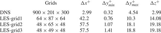A box filter is used for test filtering for the Germano identity of the dynamic procedure, where the test-filter width is 2$\varDelta$ ($\varDelta =(\varDelta _x\varDelta _y\varDelta _z)^{1/3}$). 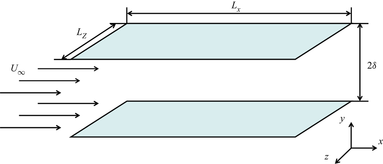Tables 1 to 4 show the grid settings and main parameters for direct numerical simulation (DNS) and LES in this case, respectively ($u_c$, $\rho _c$ and $T_c$ are the streamwise velocity, density and temperature at the midplane of the channel flow). Figure 1 shows a schematic diagram of the compressible turbulent channel flow.

Figure 1.

Schematic diagram for the compressible turbulent channel flow.

Table 1.

The grid settings and grid resolutions of the simulations in the compressible turbulent channel flow ($Ma=1.5$, $Re=3000$).

Table 2.

The main parameters for the simulations in the compressible turbulent channel flow for DNS and LES-grid1 ($Ma=1.5$, $Re=3000$).

Table 3.

The main parameters for the simulations in the compressible turbulent channel flow for LES-grid2 ($Ma=1.5$, $Re=3000$).

Table 4.

The main parameters for the simulations in the compressible turbulent channel flow for LES-grid3 ($Ma=1.5$, $Re=3000$).

First, using an $a$ $priori$ test, we will discuss the correlation of the different unclosed quantities modelled by DSM, ${{\rm d}}k$-equation model and QKM with the real values and a box filter is adopted in the streamwise and spanwise directions. The correlation coefficient is defined as

(4.1)\begin{equation} \beta=\frac{\langle (M-\langle M \rangle) (R-\langle R \rangle) \rangle}{[\langle (M-\langle M \rangle)^{2} \rangle \langle (R-\langle R \rangle)^{2} \rangle]^{1/2}}, \end{equation}

where $\langle {\cdot } \rangle$ denotes the time averaging plus space averaging in the streamwise and the spanwise directions in $a$ $priori$ tests on every plane of the turbulent channel flow.

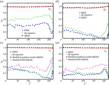
Figure 2(a–d) shows the correlation coefficients of the KEF, the wall-normal SGS heat flux, the components of SGS stress $\tau _{12}$ and $\tau _{22}$ obtained from the DSM, ${{\rm d}}k$-equation model and QKM using the $a$ $priori$ test at the scale of $6\varDelta _z$. In figure 2(a,b), we can see that all the modelled quantities from QKM have very high correlations with the real values and all the correlation coefficients are almost higher than 0.95 along the wall-normal direction. On the contrary, the correlation coefficients of these quantities from the DSM and ${{\rm d}}k$-equation model are much lower. 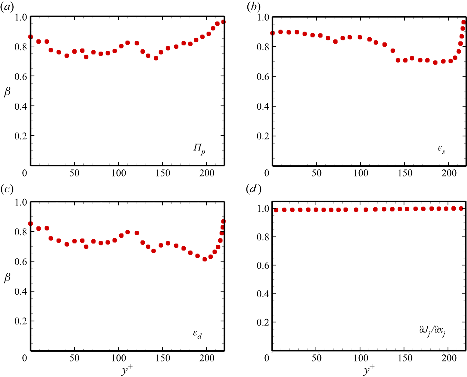Figure 2(c,d) shows that the modified gradient model from QKM still has high correlations with the real SGS stress and the modified SM has better correlations with the real values than the DSM and ${{\rm d}}k$-equation model do. We also give the correlation coefficients of the unclosed quantities in the SGS kinetic energy equation in figure 3. The correlation coefficient of the SGS turbulent diffusion term $\partial J_j /\partial x_j$ in figure 3(d) is nearly 1.0. The correlation coefficients of the other quantities (the pressure diffusion $\varPi _p$, the solenoidal dissipation $\varepsilon _s$ and the dilatational dissipation $\varepsilon _d$) are also relatively high. From all the results of the $a$ $priori$ test, we can estimate that the QKM has high similarity with the unclosed quantities in the equations.

Figure 2.

Correlation coefficients of different quantities from the DSM, ${{\rm d}}k$-equation model and QKM obtained $a$ $priori$: (a) the KEF $\varPi _{\varDelta }$; (b) the wall-normal SGS heat flux $Q_2$; (c) the component of SGS stress $\tau _{12}$; (d) the component of SGS stress $\tau _{22}$.

Figure 3.

Correlation coefficients of the different terms in the SGS kinetic equation from the QKM obtained $a$ $priori$: (a) the pressure diffusion term $\varPi _p$; (b) the solenoidal dissipation term $\varepsilon _s$; (c) the dilatational dissipation term $\varepsilon _d$; (d) the SGS turbulent diffusion term ${\partial J_j}/{\partial x_j}$.

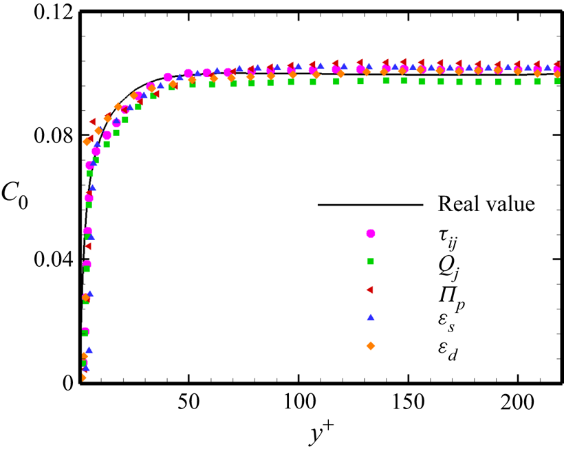
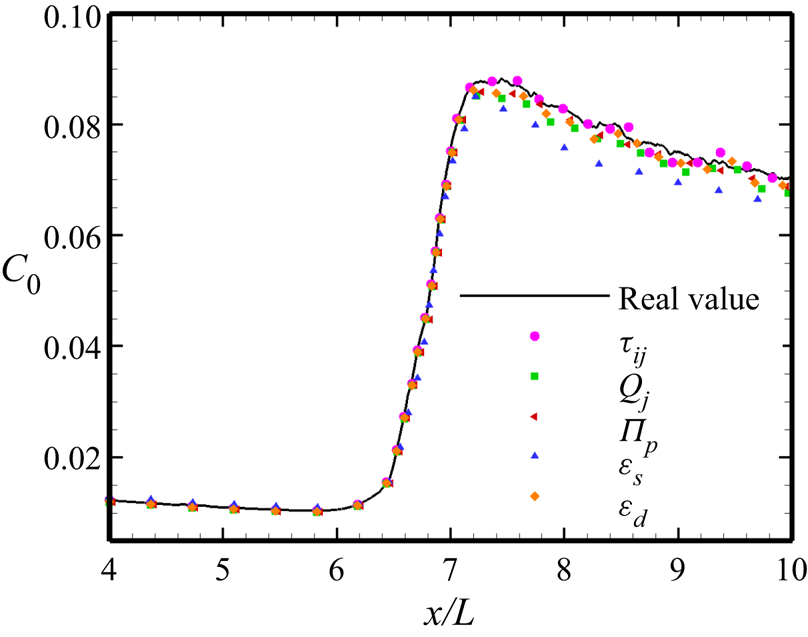
The real value of the coefficient $C_0$ obtained from (3.15) and the $C_0$ of the different expanded terms $\tau _{ij}$, $Q_j$, $\varPi _p$, $\varepsilon _s$ and $\varepsilon _d$ using the $a$ $priori$ test are displayed in figure 4. From the figure, we can see that all the profiles of $C_0$ from the expanded terms have good agreement with the profile of the real $C_0$, including the trend and value. Therefore, the $a$ $priori$ results further verify the validity of our assumption. Next, we will discuss the results of the $a$ $posterior$ test in the channel flow of $Ma=1.5$.

Figure 4.

The coefficient $C_0$ of the different expanded terms and the real value obtained $a$ $priori$ using the DNS data.

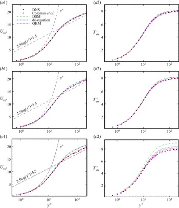
The profiles of the van Driest transformed mean velocity ($U_{vd}=\int _0^{U}\sqrt {\langle \rho \rangle /\rho _w}\,{{\rm d}}\langle {U} \rangle$) and the mean temperature $T_{av}^{+}=(T_w-\langle T \rangle )/T_{\tau }$ obtained from DNS, the QKM, the ${{\rm d}}k$-equation model and the DSM are compared for three LES grid resolutions in figure 5. Here, $T_\tau =B_q T_w$ is the friction temperature, $B_q=q_w/(\rho _w c_p u_{\tau } T_w)$ is the non-dimensional heat flux and $q_w$ is the wall-normal heat flux. For LES-grid1, shown in figure 5(a1,a2), we can see that all the SGS models can well predict the mean velocity and temperature, and the QKM behaves a little better than the other SGS models. From figure 5(b1,b2), we can see that the results from all the models on LES-grid2 and the DNS results present little difference in the viscous sub-layer and the buffer regions. However, in the log-law region, the QKM predicts the velocity profile perfectly and clearly performs better than the other two models. In figure 5(c1,c2), we can see that the results from QKM are still close to the DNS results and are obviously better than those of the other two models. In short, as the grid scale decreases, the QKM can maintain good predictive ability, which is significantly better than those of the other two models, and the ${{\rm d}}k$-equation model is better than the DSM. These results show that the QKM has a certain characteristic of scale adaptivity.

Figure 5.

The van Driest transformed mean velocity $U_{vd}$ profiles and the profiles of the mean temperature $T_{av}^{+}$, which are predicted from the DSM, ${{\rm d}}k$-equation model and QKM, are compared with those of DNS: (a1) and (a2) show the case of LES-grid1; (b1) and (b2) show the case of LES-grid2; (c1) and (c2) show the case of LES-grid3. The velocity and temperature profiles from Coleman, Kim & Moser (Reference Coleman, Kim and Moser1995) are also given here.

Next, we will perform analyses according to the results of LES-grid2 for the case of $Ma=1.5$.

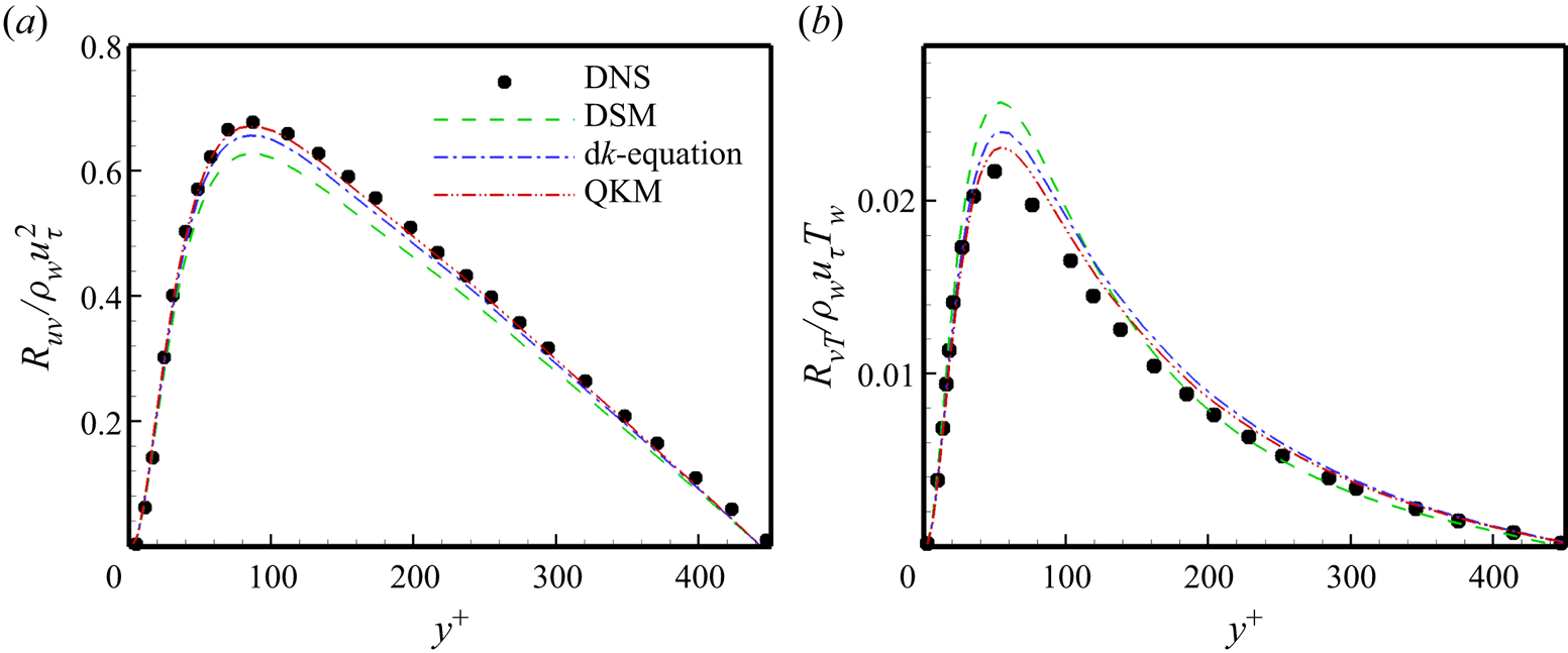
In compressible turbulence, if the property of ergodicity is assumed, the total Reynolds stress could be expressed as

(4.2)\begin{equation} R_{ij}=\langle \bar{\rho} \rangle (\{\widetilde{u_i u_j}\}-\{\widetilde{u}_i\} \{\widetilde{u}_j\})=R_{ij}^{LES}+\langle\tau_{ij}\rangle, \end{equation}

where

(4.3)\begin{equation} R_{ij}^{LES}=\langle \bar{\rho} \rangle (\{\widetilde{u}_i \widetilde{u}_j\}-\{\widetilde{u}_i\} \{\widetilde{u}_j\}) \end{equation}

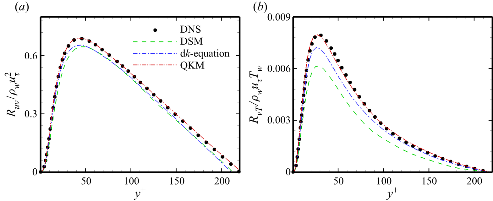
is the resolved Reynolds stress, and $\{ {\cdot }\}$ denotes the Favre averaging ($\{\phi \}={\langle \rho \phi \rangle }/{\langle \rho \rangle }$). Figure 6(a) displays the normalized total Reynolds stress $R_{uv}/(\rho _w u_{\tau }^{2})$ from DNS and the different models. In figure 6(a), the QKM shows better agreements than the other models in almost all the regions.

Figure 6.

The profiles of the total Reynolds stress normalized by $\rho _w$ and $u_{\tau }$, and the total turbulent heat flux normalized by $\rho _w$, $u_{\tau }$ and $T_w$ from DNS and different SGS models in the case of LES-grid2.

Similar to the expression of the total Reynolds stress in (4.2), the turbulent heat flux takes the form

(4.4)\begin{equation} R_{u_j T}=\langle \bar{\rho} \rangle (\{\widetilde{u_j T}\}-\{\widetilde{u}_j\} \{\widetilde{T}\})=R_{u_j T}^{LES}+\langle Q_j \rangle, \end{equation}

where

(4.5)\begin{equation} R_{u_j T}^{LES}=\langle \bar{\rho} \rangle (\{\widetilde{u}_j \widetilde{T} \}-\{\widetilde{u}_j\} \{\widetilde{T}\}) \end{equation}

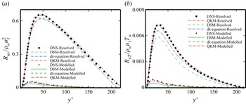
is the resolved turbulent heat flux. Figure 6(b) presents the profiles of the normalized turbulent heat flux $R_{vT}/(\rho _wu_{\tau }T_w)$ from DNS, the DSM, the ${{\rm d}}k$-equation model and the QKM. From figure 6(b), we can see that the QKM yields a precise prediction compared with the DNS, but the other models still have obvious deviations from the real value. And we also show the resolved Reynolds stress and the resolved turbulent heat flux in figure 7. From the figures, we see that the QKM can predict both the resolved part and the modelled part well. The ${{\rm d}}k$-equation model can also obtain better results than the DSM does.

Figure 7.

The profiles of the resolved Reynolds stress normalized by $\rho _w$ and $u_{\tau }$, and the resolved turbulent heat flux normalized by $\rho _w$, $u_{\tau }$ and $T_w$ from DNS and different SGS models in the case of LES-grid2.

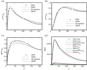
In figure 8(a–c), we present the profiles of the normalized resolved turbulence intensities $\widetilde {u}_i ^{rms}/u_{\tau }=\langle (\widetilde {u}_i-\langle \widetilde {u}_i\rangle )^{2} \rangle ^{1/2}/u_{\tau }$ obtained from the DNS and the compared SGS models. From figure 8, the three components of the resolved turbulence intensity predicted by the QKM are clearly much closer to the real values than those from the DSM and d$k$-equation model in all regions. Figure 8(d) shows the turbulent kinetic energy from DNS and the different models. From the figure, we see that the QKM can supply better results than the other SGS models including the total turbulent kinetic energy and $\rho k_{sgs}$.

Figure 8.

The profiles of the resolved turbulence intensities normalized by the friction velocity $u_{\tau }$ and the turbulent kinetic energy (TKE) from DNS and different SGS models in the case of LES-grid2: (a) streamwise turbulence intensity; (b) wall-normal turbulence intensity; (c) spanwise turbulence intensity; (d) the TKE $\frac {1}{2}R_{ii}$.

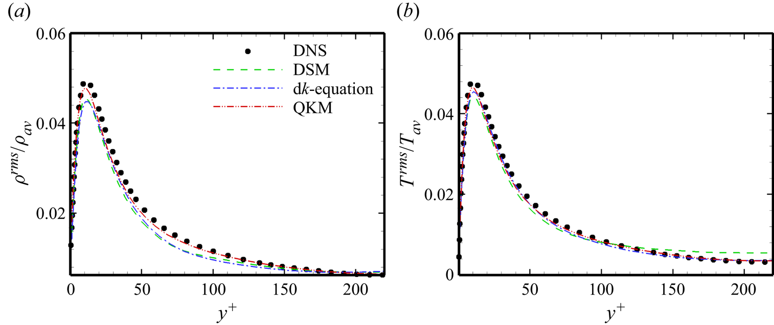
In compressible channel flows, density and temperature fluctuations also attract much attention. The profiles of the normalized resolved density fluctuation $\rho ^{rms}/\rho _{av}$ and temperature fluctuation $T^{rms}/T_{av}$ predicted from DNS and the different SGS models are shown in figure 9, where $\rho _{av}$ and $T_{av}$ are the average density and temperature, respectively. As expected, the density and temperature fluctuations obtained from the QKM tightly match the profiles from DNS, which is a little better than the results of the other SGS models.

Figure 9.

The profiles of the resolved root-mean-square (r.m.s.) density fluctuations normalized by averaged density $\rho _{av}$ and the resolved r.m.s. temperature fluctuations normalized by averaged temperature $T_{av}$ from DNS and different SGS models in the case of LES-grid2: (a) density fluctuations; (b) temperature fluctuations.

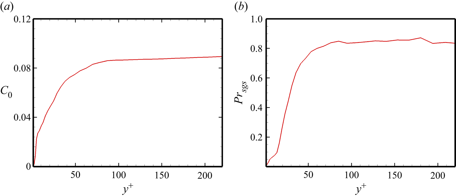
Next, we show the profiles of $C_0$ and $Pr_{sgs}$ from the $a$ $posteriori$ test in figure 10. The values of $C_0$ and $Pr_{sgs}$ have similar trends. Notably, the maximum value of $C_0$ is approximately 0.08 and the maximum value of $Pr_{sgs}$ is approximately 0.8.

Figure 10.

The profiles of $C_0$ and $Pr_{sgs}$ obtained $a$ $posteriori$ for the compressible turbulent channel flow in the case of LES-grid2.

Then we compare the turbulent structure obtained from DNS and the different SGS models. Figure 11 shows the instantaneous isosurface of $Q$ (second invariant of the strain-rate tensor, $Q=0.25$) obtained from DNS, the QKM, the DSM and the ${{\rm d}}k$-equation model. From figure 11, we can see that the QKM can predict more abundant structures, and in figure 11(b) there are many more small-scale vortexes than the results in figure 11(c,d), especially in the near-wall regions. Therefore, we infer that the QKM has a better ability to predict the turbulent structure.

Figure 11.

Instantaneous isosurface of $Q$ (second invariant of the strain-rate tensor, $Q=0.25$) obtained from (a) DNS, (b) the QKM, (c) the DSM, (d) the ${{\rm d}}k$-equation model of compressible turbulent channel flow in the case of LES-grid2.

To see the computational efficiency of the SGS models, we show the computing time per time step using 112 CPUs from different SGS models in table 5. Obviously, the QKM and ${{\rm d}}k$-equation model take approximately the same time, slightly longer than the DSM.

Table 5.

The computing time per time step using 112 CPUs for different SGS models.

Table 6.

The grid settings and grid resolutions of the simulations in the compressible turbulent channel flow ($Ma=3.0$, $Re=4880$).

Table 7.

The main parameters for the simulations in the compressible turbulent channel flow ($Ma=3.0$, $Re=4880$).

To further test the new model in the case of a higher Mach number, we will discuss the results for the case of $Ma=3.0$ and $Re=4880$ (Coleman et al. Reference Coleman, Kim and Moser1995; De Stefano, Brown-Dymkoski & Vasilyev Reference De Stefano, Brown-Dymkoski and Vasilyev2020). The size of the computational domain, the Prandtl number $Pr$, the boundary conditions, the ratio of specific heats and the setting of LES solver are the same with the case of $Ma=1.5$ and $Re=3000$. The grid resolutions and the main parameters of this case are listed in tables 6 and 7, respectively.

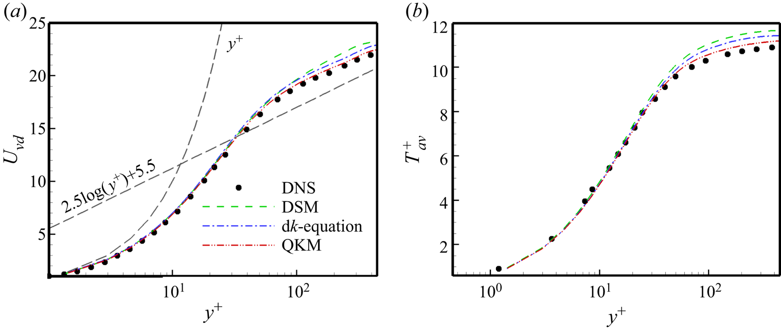
Figure 12 shows the profiles of the van Driest transformed mean velocity $U_{vd}$ and mean temperature $T_{av}^{+}$ obtained from different SGS models and DNS. Figure 13 shows the profiles of the total Reynolds stress and the turbulent heat flux normalized by $\rho _w$, $u_{\tau }$ and $T_w$ from different SGS models and DNS. From the figures, we can see that the QKM can yield obviously better behaviour than the other models even in the case of higherMach number. At the same time, the ${{\rm d}}k$-equation model can supply better predictions than the DSM.

Figure 12.

The profiles of the van Driest transformed mean velocity $U_{vd}$ and mean temperature $T_{av}^{+}$ obtained from different SGS models and DNS. The DNS results are from Coleman et al. (Reference Coleman, Kim and Moser1995).

Figure 13.

The profiles of the total Reynolds stress and the turbulent heat flux normalized by $\rho _w$, $u_{\tau }$ and $T_w$ from different SGS models and DNS. The DNS results are from Coleman et al. (Reference Coleman, Kim and Moser1995).

4.2. Application in compressible flat-plate boundary layer

In this part, the newly proposed model is tested in the flow of the compressible flat-plate boundary layer. Unlike the channel flow, the compressible flat-plate boundary layer flow contains laminar, transitional and fully turbulent regions. Here, a typical spatially developing supersonic flat-plate boundary layer flow (Pirozzoli, Grasso & Gatski Reference Pirozzoli, Grasso and Gatski2004) is chosen as a standard example. The simulation results from the DSM and ${{\rm d}}k$-equation model are also selected for comparison. The computational domain is set to the same in-flow and out-flow boundary conditions as the standard example, the no-slip condition is used in the wall and the periodic condition is applied in the spanwise direction. Also, $L$ (one inch) is the non-dimensionalizing length scale. Blow and suction disturbances are imposed near the wall at $4.5< x/L<5.0$ to trigger the transition, which is the same as the standard example except for the amplitude of the disturbances (0.02 is selected here). 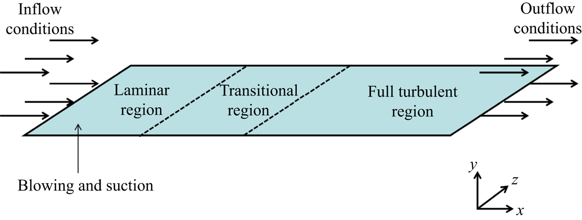The size of the computational domain is $L_x\times L_y\times L_z=6\times 0.3\times 0.175$. The sketch of the computational domain is shown in figure 14. The Mach number $Ma=2.25$ and the free-stream unit Reynolds number $Re/in.= 635\,000$ are selected for this case. The grid resolution for DNS in this case is $10\,000\times 90\times 320$ with a spatial resolution of ${\rm \Delta} x^{+}=6.02, {\rm \Delta} z^{+}=5.47$, and minimum grid spacing in the wall-normal direction ${\rm \Delta} y_w^{+}=0.58$. Three different LES grid settings are selected for testing the models and the main parameters of the simulation in the compressible flat-plate boundary layer are listed in table 8.

Figure 14.

Sketch of the computational domain for the compressible flat-plate boundary layer.

Table 8.

The grid settings and main parameters of the simulations in compressible flat-plate boundary layer ($Ma=2.25$, $Re/in.=635\,000$).

First, we test the rationality of our assumption regarding $C_0$ in the compressible flat-plate boundary layer using the $a$ $priori$ test with DNS data at the scale of $3\varDelta _z$ from the compressible flat-plate boundary layer in figure 15. From the figure, we can see that the values of $C_0$ obtained from the different expanded terms ($\tau _{ij}$, $Q_j$, $\varPi _p$, $\varepsilon _s$ and $\varepsilon _d$) still have a similar trend and value as the real results. The results from the $a$ $priori$ test confirm the validity of our assumption.

Figure 15.

The profiles of $C_0$ along the streamwise direction at $y^{+}=15$ using the $a$ $priori$ test in the compressible flat-plate boundary layer.

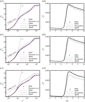
The distributions of the van Driest transformed mean velocity at $x/L=8.8$ and the skin friction coefficient along the flat plate obtained from the different SGS models in three LES cases and DNS are displayed in figure 16. From figure 16(a1,a2) we can see that the results from the QKM precisely accord with the real values. The DSM and ${{\rm d}}k$-equation model can also supply passable prediction results, including the mean velocity profile, the transition onset and the transition peak. For the case of grid-B, as seen from the simulation results in figure 16(b1,b2), the QKM can still supply accurate prediction results that are much better than those obtained from the DSM and ${{\rm d}}k$-equation model. The results from the ${{\rm d}}k$-equation model are better than those from the DSM. In the case of grid-C, the grid has the lowest resolution. Figure 16(c1,c2) shows that the QKM can still provide fairly good results, while the other two models cannot yield acceptable simulation results. Overall, from the results in figure 16, we could infer that the QKM can predict the mean quantities in compressible flat-plate boundary layer flow properly and that it also has good scale adaptivity.

Figure 16.

The profiles of the van Driest transformed mean velocity at $x/L=8.8$ and the skin friction coefficient distribution along the flat plate from different SGS models and DNS: (a1) and (a2) show grid-A; (b1) and (b2) show grid-B; (c1) and (c2) show grid-C. The velocity profile from Pirozzoli et al. (Reference Pirozzoli, Grasso and Gatski2004) is also given here.

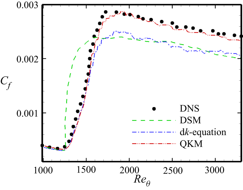
Next, we will use the results from the case of grid-C to further explore the characteristics of the QKM. To further observe the prediction of the transition, we supply the profiles of the skin friction coefficient distribution vs $Re_{\theta }$ ($Re_{\theta }=\rho _{\infty } u_{\infty } \theta /\mu _{\infty }$ is a momentum thickness Reynolds number) from different SGS models and DNS in the case of grid-C in figure 17. The QKM maintains the best performance in predicting the transition onset and the transition peak, and the ${{\rm d}}k$-equation model can also predict the transition process except the transition peak, but the prediction results of the DSM deteriorate distinctly.

Figure 17.

Profiles of skin friction coefficient distribution versus $Re_{\theta }$ from different SGS models and DNS in the case of grid-C.

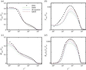
In figure 18, we show the profiles of the normalized resolved turbulence intensities and the turbulent heat flux at $x/L=8.8$ from the different SGS models and DNS in the case of grid-C. We can see that the streamwise turbulence intensities from the QKM, DSM and ${{\rm d}}k$-equation model in figure 18(a) show no great difference, but the QKM shows better performance at $y^{+}<10$. The wall-normal and spanwise turbulence intensities in figures 18(b) and 18(c) have different behaviours and the results from the QKM are better than those from the other models. The ${{\rm d}}k$-equation model behaves better than the DSM. From figure 18(d), we can see that the QKM could predict the turbulent heat flux well and that its results are better than those of the DSM and ${{\rm d}}k$-equation model.

Figure 18.

Profiles of the resolved turbulence intensities normalized by $U_{av}$ and the turbulent heat flux normalized by $\rho _w U_{av} T_{av}$ at $x/L=8.8$ from different SGS models and DNS in the case of grid-C: (a) streamwise turbulence intensity; (b) wall-normal turbulence intensity; (c) spanwise turbulence intensity; (d) the turbulent heat flux.

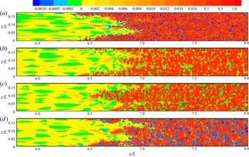
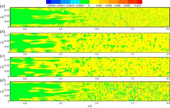
Figure 19 shows the $a$ $posteriori$ result of the KEF at $y^{+}=15$ from the different SGS models in the case of grid-C and the DNS value is displayed here for comparison (the KEF in figure 19(a) is from (3.2), and $\tau _{ij}$ is from (2.8)). From the figures, we can see that the QKM is much more similar to the real KEF than to the KEF from the other two models, including the distribution, the intensity, the sophisticated flow structure and even the energy backscatters. Similar to the prediction results of the KEF, the wall-normal SGS heat flux at $y^{+}=15$ (figure 20) predicted by the QKM shows much better behaviour than those of the other models compared with the real result (the SGS heat flux in figure 20(a) is from (2.9)).

Figure 19.

The $a$ $posteriori$ test of the KEF at $y^{+}=15$ from different SGS models in the case of grid-C and DNS results are displayed here for comparison: (a) DNS; (b) the DSM; (c) the ${{\rm d}}k$-equation model; (d) the QKM.

Figure 20.

The $a$ $posteriori$ test of the wall-normal SGS heat flux at $y^{+}=15$ from different SGS models in the case of grid-C and DNS results are displayed here for comparison: (a) DNS; (b) the DSM; (c) the ${{\rm d}}k$-equation model; (d) the QKM.

4.3. Application in spherical converging Richtmyer–Meshkov instability

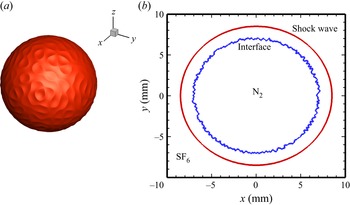
In this section, we will test the proposed model in the flow of spherical converging Richtmyer–Meshkov instability, which is a complicated time-developing case. As shown in figure 21, the shock wave converges from the heavy fluid into the light fluid in the flow. The heavy fluid is sulphur hexafluoride (SF₆) and the light fluid is nitrogen (N₂). In this case, the Mach number is approximately 1.5, and the Atwood number is $A=(\rho _h-\rho _l)/(\rho _h+\rho _l)=0.678$, where $\rho _h$ and $\rho _l$ are the densities of SF₆ and N₂ at the initial time, respectively. 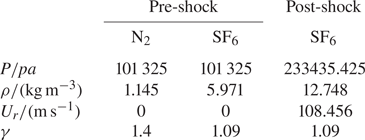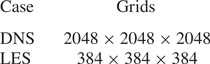The main computational domain in the Cartesian coordinate system is $L_x=L_y=L_z=20\,{\rm mm}$. The total uniform and structured Cartesian grid is applied in the main computational domain. To avoid the influence of boundary reflection, a sufficiently long sponge layer with 50 non-uniform coarse grids is added for each direction. To make sure that there is no singularity on the spherical surface, the spherical harmonic function is used to generate the initial perturbation (Lombardini, Pullin & Meiron Reference Lombardini, Pullin and Meiron2014). The main parameters at the initial time and the grid setting of the simulations in the spherical converging Richtmyer–Meshkov instability are listed in tables 9 and 10, respectively.

Figure 21.

The isosurface of $Y_{SF_{6}}=0.99$ for the spherical converging Richtmyer–Meshkov instability, and the shock wave and interface configuration diagram at the initial time: (a) isosurface of $Y_{SF_{6}}=0.99$; (b) shock wave and interface configuration diagram.

Table 9.

The main parameters at the initial time ($U_r$ is radial velocity).

Table 10.

The grid setting and the main parameters of the simulations in spherical converging Richtmyer–Meshkov instability (the Mach number is approximately 1.5, and the Atwood number is 0.678).

The N–S equations are solved by the finite difference method. The mixing scheme combining the sixth-order monotonicity preserving optimized scheme (OMP6) (Li, Yan & He Reference Li, Yan and He2013) and eighth-order central difference scheme is adopted to discretize the convective terms. The eighth-order central difference scheme is employed for the viscous terms, and the third-order Runge–Kutta approach is taken for the time integration (Hill, Pantano & Pullin Reference Hill, Pantano and Pullin2006; Bin et al. Reference Bin, Xiao, Shi, Zhang and Chen2021).

The filtered N–S equations are the same as (2.1)–(2.3). For solving the spherical converging Richtmyer–Meshkov instability, the filtered equation for the mass fraction of species (Hill et al. Reference Hill, Pantano and Pullin2006; Lombardini et al. Reference Lombardini, Hill, Pullin and Meiron2011) is introduced as

(4.6)\begin{equation} \frac{\partial \bar{\rho}\tilde{Y}_k}{\partial t}+\frac{\partial \bar{\rho}\tilde{Y}_k\tilde{u}_j}{\partial x_j}=\frac{\partial}{\partial x_j}\left(\bar{\rho}D_{km} \frac{\partial \widetilde{Y}_k}{\partial x_j}-Y_{j,k}^{sgs}\right), \end{equation}

where $Y_k$ is the mass fraction of species $k$, $D_{km}$ denotes the mixture diffusion coefficients of species $k$ which are obtained from the Schmidt number $Sc_k=\mu (\widetilde {T})/\bar {\rho } D_{km}=1$, and the SGS species flux $Y_{j,k}^{sgs}=\bar {\rho }(\widetilde {Y_k u_j}-\widetilde {Y}_k \widetilde {u}_j)$ is an unclosed term, which can be modelled as

(4.7)\begin{equation} Y_{j,k}^{sgs}={-}\frac{\mu_{sgs}}{Sc_{sgs,k}}\frac{\partial \widetilde{Y}_k}{\partial x_j}, \end{equation}

where $\mu _{sgs}$ is the SGS eddy viscosity and $Sc_{sgs,k}$ is the SGS Schmidt number.

Similar to the solution process of $Pr_{sgs}$, $Sc_{sgs,k}$ for the newly proposed model can be obtained as

(4.8)\begin{equation} Sc_{sgs,k}={-}\frac{\partial \left(\nu_{sgs}\dfrac{\partial \widetilde{Y}_k}{\partial x_j}\right)/ \partial x_j}{\partial \left(C_0\varDelta_m^{2} \dfrac{\partial \widetilde{u}_j}{\partial x_m}\dfrac{\partial \widetilde{Y}_k}{\partial x_m}\right)/\partial x_j}. \end{equation}

The constant-coefficient SM is also selected for comparison here. The model coefficient of the SM is chosen as 0.1. $Pr_{sgs}$ and $Sc_{sgs,k}$ for the constant-coefficient model are set as 0.9 and 0.35, respectively.

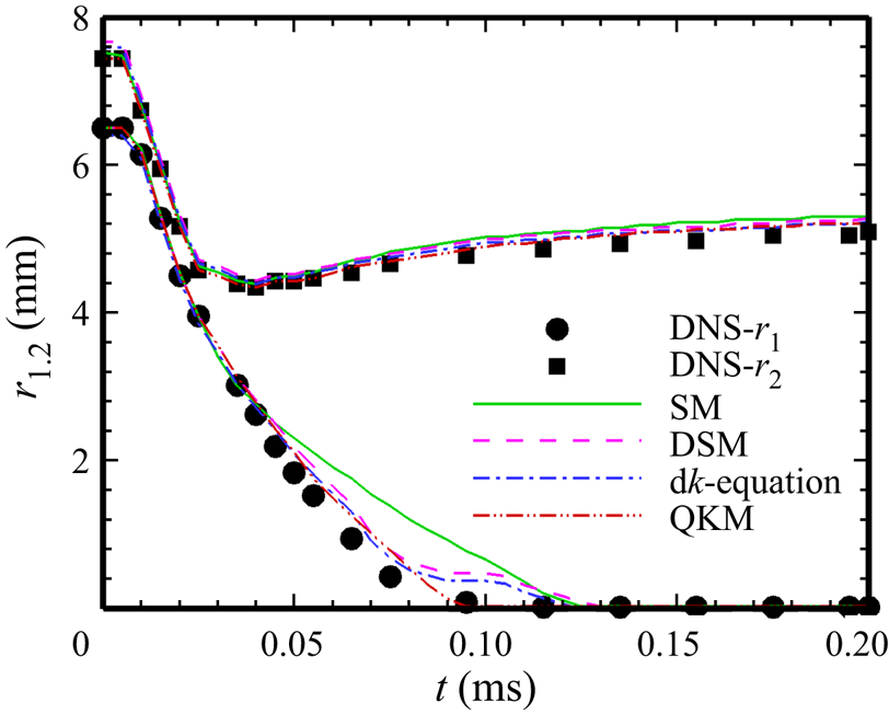
Figure 22 shows the evolution of the inner and outer radii of the mixing layer with the time obtained from different models and DNS. The inner radius $r_1$ is the position where the mass fraction of the heavy fluid is 0.01 and the outer radius $r_2$ is the position where the mass fraction of the light fluid is 0.01. For the inner radius, the QKM can obtain proper results at almost time, DSM and ${{\rm d}}k$-equation model show deviation from the DNS result during $0.075\,{\rm ms}< t<0.12\,{\rm ms}$, and the SM shows worse prediction during $0.04< t<0.12$ ms. For the outer radius, the QKM can accurately predict the evolution profile and still perform better than the DSM, ${{\rm d}}k$-equation model and SM. The DSM and ${{\rm d}}k$-equation model have better predictions than the SM in most of area.

Figure 22.

The evolution of the inner and outer radii of the mixing layer with the time obtained from different SGS models and DNS.

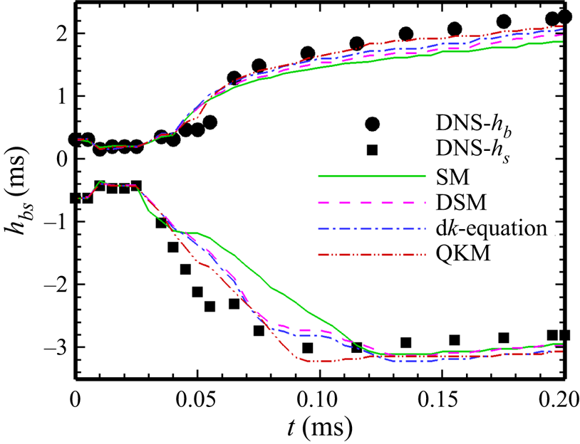
Then, the evolution profiles of the heights of the bubble (where light fluid penetrates heavy fluid) and spike (where heavy fluid penetrates light fluid) obtained from DNS and the different SGS models are compared in figure 23. According to the inner and outer radii of the mixing layer, the heights of the bubble and spike are given as

(4.9)$$\begin{gather} h_b=r_2-r_{0.5}, \end{gather}$$

(4.10)$$\begin{gather}h_s=r_1-r_{0.5}, \end{gather}$$

where $r_{0.5}$ is the position where the mass fractions of light and heavy fluids are both 0.5. The SM cannot predict the heights of the bubble and spike, and it grossly underestimates their values, especially during $0.04< t<0.12$ ms. In contrary, the QKM can still yield passable results during the whole process.

Figure 23.

The evolution of the heights of the bubble and spike with the time obtained from different SGS models and DNS.

From figures 22 and 23, we could infer that the turbulent mixing begins at $t=0.04$ ms and ends at 0.12 ms, which accords with the conclusion that the SM cannot successfully predict the transition process (Piomelli & Zang Reference Piomelli and Zang1991; Meneveau & Katz Reference Meneveau and Katz2000; Sayadi & Moin Reference Sayadi and Moin2012; Zhou et al. Reference Zhou, Li, Qi and Yu2019). At the same time, we can see that the results from the DSM and ${{\rm d}}k$-equation model show deviation from DNS results during $0.075\,{\rm ms}< t<0.12\,{\rm ms}$, obviously. Perhaps, it is caused by strong anisotropy and inhomogeneity of the flow during $0.075\,{\rm ms}< t<0.12\,{\rm ms}$, which cannot meet the requirement of scale invariance for the traditional dynamic procedure. And it also proves that the QKM can predict the turbulent mixing process well.

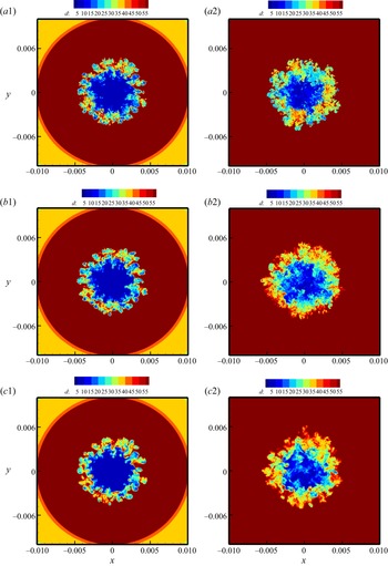
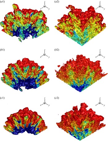
Then, we select the results of the density distribution in the $x$–$y$ plane and the isosurfaces of the mass fraction of SF₆ from DNS, QKM and the SM at two moments ($t=0.08$ and $t=0.12$ ms), shown in figures 24 and 25. From figures 24 and 25, we can see that the QKM is much more similar to DNS than the SM, including the spatial distributions of the different species and the locations of the converging surfaces. We have seen again that the QKM can provide sufficiently abundant turbulent structures.

Figure 24.

The density distribution in the $x$–$y$ plane: (a1,b1,c1) are at $t=0.08$ ms; (a2,b2,c2) are at $t=0.2$ ms; (a1,a2) are from DNS; (b1,b2) are from the QKM; (c1,c2) are from the SM.

Figure 25.

The isosurfaces of the mass fraction of SF₆: (a1,b1,c1) are at $t=0.08$ ms; (a2,b2,c2) are at $t=0.2$ ms; (a1,a2) are from DNS; (b1,b2) are from the QKM; (c1,c2) are from the SM (Only one eighth of the main computational domain is shown).