

1 Introduction
The economic policy varied substantially over the years that General Franco remained in power (1939-1975). During its early years, the new regime introduced a set of anti-market policies that altered the previous behaviour of the Spanish economy dramatically. These measures resulted in high inflation rates, the development of «black markets» and a contraction in international trade. In a subsequent phase, during the 1950s, the most extreme interventionist policies were relaxed, while the Spanish economy benefited from a (military and technological) cooperation agreement with the U.S. government. A critical economic situation by mid-1959, in particular a shortage of foreign reserves, induced more drastic economic reforms. The authorities presented this set of reforms as a package, the Liberalisation and Stabilisation Plan (hereafter PSL). Simultaneously, Spain joined major international organisations increasingly committing the government to the free market discipline. As a consequence, inflation decreased, «black markets» disappeared, foreign investment increased and international trade flourishedFootnote 1.
Our main goal is to test the impact of Franco's economic policies on Spanish economic growth quantitatively. In particular, we will revisit the widespread claim that the new policies associated with the 1959 PSL had a dramatic impact on Spain's growth performance and explore the effects on growth of the previous tentative steps to soften regulation and intervention. A market-oriented reform is a policy measure that favours the competitive participation of private agents in economic activity, and thus assessing the impact of policy reforms is not an easy task and there are many ways to go about it (see Loayza and Soto Reference Loayza and Soto2003). Our choice has been to construct an index of macroeconomic distortions (hereafter IMD) and analyse its impact on growth in several counterfactual scenarios.
In a nutshell, our results confirm the important role played by the PSL and the subsequent reforms in promoting sustained economic growth while stressing the permissive role played by the gradual and moderate reduction of macroeconomic distortions during the 1950s. According to our calculations, without these successive economic policy reforms, GDP would have been significantly lower at the time of Franco's death in 1975.
The rest of the paper is organised as follows. Section 2 reviews Franco's regime growth record and its economic policy. In section 3, we introduce the IMD, which allows us to determine major economic policy changes in SpainFootnote 2. Then, in section 4, we examine, with the help of a structural model, the main determinants of growth, highlighting the deterrent role played by macroeconomic distortions. As a sensitivity test, in section 5, we investigate the economic impact of macroeconomic restrictions using a vector autoregression (VAR) approach. In both sections 4 and 5, the economic cost of early Francoism anti-market policies is assessed by exploring alternative counterfactual scenarios; and section 6 is the conclusion.
2 Economic Performance and Policy during Franco's Regime
Economic performance during General Franco's dictatorship represents an exception in the economic history of Modern Spain (Figure 1). Franco's regime covered the period from the end of the Civil War (1936-1939) to the dictator's death in 1975. A closer look reveals that, after the contraction that resulted from the Civil War and a very slow recovery during the 1940s, per capita GDP growth intensified in the 1950s and accelerated dramatically from the 1959 PSL up to 1974.
REAL PER CAPITA GDP, 1850-2000 (000 PESETAS) (2000 PRICES)
Sources: Prados de la Escosura (Reference Prados de la Escosura2003, updated).

In comparative perspective, during the early phase of Franco's dictatorship, Spain's growth record was highly disappointing. Spain did not recover its pre-Civil War per capita GDP peak levels (1929) until 1955, while Western European countries reached, on average, 1938 levels of GDP per head by 1950. Such a difference is more striking given that the destruction of lives and physical capital, as a consequence of the Spanish Civil War, was lower than in most of Western European countries involved in the World War IIFootnote 3. However, an intense destruction of human capital occurred as a result of political exile and post-war political repression (see López García Reference López García1991; Prados de la Escosura Reference Prados de la Escosura2007; Prados de la Escosura and Rosés Reference Prados de la Escosura and Rosés2010b). The situation began to change in the 1950s when, in per capita terms, the Spanish economy grew at a similar rate to the Western European average, but with the significant difference that Spain started from a substantially lower levelFootnote 4. It was during the last period of Franco's rule (1959-1975) when per capita GDP growth reached an unprecedented intensity in Spain, not far behind that of 1950s Germany and significantly above Western Europe and the United States.
At first sight, significant differences in the forces behind economic growth can be observed between the three periods mentioned above (Table 1). In the earlier period, 1939-1951, per capita income growth (2.1 per cent) depended, almost equally, on the increase in GDP per hour worked (0.9 per cent per year) and on the rise in hours worked per person (1.1 per cent). Efficiency gains explained, in turn, all the improvement in labour productivity. In the second period, 1952-1958, per capita GDP growth accelerated (4.4 per cent) depending exclusively on the increase in labour productivity (4.2 per cent), which largely resulted from efficiency gains (2.6 per cent), but also from broad capital deepening. The pattern initiated in the 1950s intensified during 1959-1975, with labour productivity (6.4 per cent) accounting for all the improvement in per capita GDP (5.6 per cent), while the rise in total factor productivity (4.2 per cent) accounts for two-thirds of the increase in output per hour worked.
SPAIN'S ECONOMIC GROWTH AND ITS SOURCES

Sources: Prados de la Escosura and Rosés (Reference Prados de la Escosura and Rosés2009).
Why was the economic growth record so disappointing during the early period of Franco's rule? Why did the economy grow during the 1950s with no apparent significant transformation of the political regime? What does account for the acceleration in Spain's pace of growth since 1960?
The early years of the dictatorship — from the Civil War up to the early 1950s — represented a dramatic rupture with the economic policies prevalent in Spain from the mid-19th century. Effective possession of legislative and judicial powers gave Franco's dictatorship the ability to alter economic and political rights discretionally. The dictatorship did not reassure economic agents of the New State's commitment to private property and the free market. Quite the contrary, the new authorities shared a strong anti-market attitude and their economic policy often threatened private initiative and investment (Fraile Balbín Reference Fraile Balbín1998). Severe market controls aimed at economic autarchy were implemented (Barciela Reference Barciela2002). The new state-owned enterprises began by controlling «strategic» industries seeking technical solutions to maximise the amount of production, bypassing the opportunity cost of their decisions (Martín Aceña and Comín Reference Martín Aceña and Comín1991). Labour relations were subordinated to the «national interest» and employers and workers incorporated into a single «vertical» union in an attempt to harmonise diverging social and economic interests (González Reference González1979). This economic policy provided, in turn, an advantageous position to those small groups and coalitions which, in exchange for support to the dictatorship, would derive rents from the public sector and even control the state's economic decisions (Fraile Balbín Reference Fraile Balbín1999). To make the economic situation even worse, economic agents were uncertain about how long the regime would last (Calvo-González Reference Calvo-González2001, Reference Calvo-González2007a).
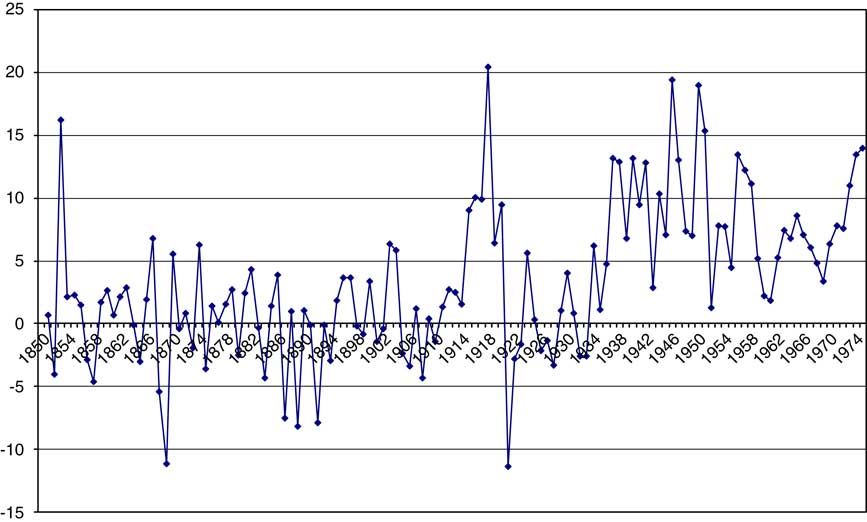
Although the size of the government increased (Figure 2), no tax reform to boost its revenues was introduced until 1957, as apparently a clash with interest groups supporting the regime was feared (Díaz Fuentes Reference Díaz Fuentes1994; Comín Reference Comín1996). Thus, a large amount of debt was issued while a policy of low nominal interest rates was implemented. In addition, limits to fiduciary circulation were suspended and the Bank of Spain was given full power for proceeding with debt monetisation. Under these circumstances, monetary policy succumbed to the demands of the government budget (Martín Aceña Reference Martín Aceña1994). Clearly, the potential inflationary risks of this new monetary management were very high, since any increase in public debt could determine a monetary expansion. In consequence, inflation rates were comparatively high during the early years of Franco's rule even though inflation was repressed through officially established prices (Figure 3). The inflation rate was, on average, 10 per cent higher than that of the 1940s. It decreased to 8 per cent in the 1950s, and after the stabilisation measures inflation rates practically halved, falling below 6 per cent, on average, during 1959-1973, and only went up to 12 per cent after the 1973 oil shockFootnote 5.
SHARE OF GOVERNMENT CONSUMPTION IN TOTAL CONSUMPTION, 1850-1975
Sources: Prados de la Escosura (Reference Prados de la Escosura2003) and see the text.

INFLATION RATE, 1850-1975 (%)
Sources: Prados de la Escosura (Reference Prados de la Escosura2003) and see the text.
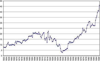
Franco's regime also represented an exception from the point of view of Spain's integration in the international economy as it started with a dramatic closing down followed, after the stabilisation plan of 1959, by opening up to a historical maximum (Figure 4). The new regime strongly regulated foreign currency markets aiming at having absolute control of foreign trade (Martínez Ruiz Reference Martínez Ruiz2003). The private possession of foreign currency was prohibited and exporters forced to hand it over to the Spanish Institute for Foreign Currency (IEME) at the official, overvalued exchange rateFootnote 6. The overvaluation of the exchange rate, a matter of national pride for the Franco regime, harmed exports and fed the desire to import. To avoid collapse, the regulation and control of currency trade was very strict. The outcome of all these policies was a strong premium for currency exchange in the «black market», and thus a substantial deviation between the official and the free market exchange rate of the pesetaFootnote 7.
OPENNESS, 1850-2000 (EXPORTS AND IMPORTS AS % OF GDP)
Sources: Prados de la Escosura (Reference Prados de la Escosura2003).

During the 1950s, economic interventionism was relaxed, but not suppressed, and the international isolation Spain had suffered since 1945, due to Franco's alignment with the Axis powers during the World War II, began to decrease. Thus, the centralised allocation of scarce goods, namely food rationing and quotas for raw materials and energy, was abolished (Barciela Reference Barciela2002). Yet, foreign investment continued to be harshly restricted (Viñas et al. Reference Viñas, Viñuela, Eguidazu, Fernández Pulgar and Florensa1979; Barciela Reference Barciela2002; Martínez Ruiz Reference Martínez Ruiz2003). The new international context dominated by the Cold War helped decisively to rehabilitate the regime of General Franco in the international community. In November 1950, the United States supported a vote in the U.N. General Assembly invalidating the 1946 resolution, which excluded Spain from this organisation, while the Pact of Madrid (September 1953) committed the United States to provide an unspecified amount of aid in return for the right to establish four military bases in Spain (Calvo-González Reference Calvo-González2006)Footnote 8. In the 1950s, fast and intensive growth was apparently facilitated by the increasing confidence of economic agents derived from the greater political stability that followed the U.S.–Spain cooperation agreements (Calvo-González Reference Calvo-González2007a).
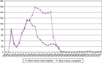
Reforms also arrived at the foreign exchange market. In an attempt to dampen the negative effects of the prevalent exchange rate policy, the authorities adopted a system of multiple exchange rates in 1948, which lasted until July 1959 (Figure 5). This new system, designed to facilitate exports and imports of certain goods by applying favourable exchange rates, has been accused of hindering foreign trade and increasing corruption (Donges Reference Donges1976; de la Dehesa et al. Reference De la Dehesa, Ruíz and Torres1991). Yet, the multiple exchange rate system allowed the authorities to devalue the peseta surreptitiously (Serrano Sanz and Asensio Castillo Reference Serrano Sanz and Asensio Castillo1997). Thus, when computed with the official — and practically fixed — exchange rate, the « black market» premium increased between 1948 and 1956. However, when an «effective» official exchange rate — derived by weighting different official exchange rates by its relative importance within the balance of payments on current account — is considered, a gradual convergence is found between the free and the «effective» official exchange rate, with a subsequent contraction in the « black market» premium (see Serrano Sanz and Asensio Castillo (Reference Serrano Sanz and Asensio Castillo1997) and especially Martínez Ruiz Reference Martínez Ruiz2003).
«BLACK MARKET» PREMIUM 1939-1975: TRADE-WEIGHTED AND UNWEIGHTED
Sources: Computed from Serrano Sanz and Asensio Castillo (Reference Serrano Sanz and Asensio Castillo1997), Martínez Ruiz (Reference Martínez Ruiz2003), Reinhart and Rogoff (Reference Reinhart and Rogoff2004), Martín Aceña and Pons (Reference Martín Aceña and Pons2005).

In the late 1950s, there were clear signs of economic overheating such as growing inflation and increasing external deficit. In particular, foreign exchange reserves were exhausted by mid-1959. In such circumstances, a complete economic policy reorientation, represented by the PSL, took place. Spain opened up to major international organisations and committed to gradual liberalisationFootnote 9. Spanish presence in major international organisations was an implicit guarantee of the definitive abandonment of isolationist options, legitimised the change in economic policy, facilitated the arrival of foreign technical assistance and reduced the opposition to economic reforms from within Franco's regime (Sardà Reference Sardà1970; González Reference González1979; Fuentes Quintana Reference Fuentes Quintana1984; Varela Parache Reference Varela Parache2004)Footnote 10.
The 1959 PSL marked the beginning of a new era in the Spanish economy as the country entered a process of economic liberalisation and international market integration. Measures in three main areas deserve highlighting. Firstly, a classical stabilisation operation was executed with the objective of reducing inflation, which was mainly due to a lack of monetary discipline. Public spending was controlled, the issue of new public debt limited and the Bank of Spain's discount rate increased. Secondly, domestic markets were partly liberalised by suppressing regulations and simplifying administrative procedures. Prices of goods (petrol, tobacco) and services (telephone, transport) supplied by state monopolies were adjusted upwards in an attempt to close the gap between official prices and their real provision costs. Lastly, a liberalisation of foreign economic relations was implemented (Fuentes Quintana Reference Fuentes Quintana1984; de la Dehesa et al. Reference De la Dehesa, Ruíz and Torres1991). In July 1959, Spanish authorities liberalised 50 per cent of the nation's trade. Eventually the recurrent financial problems due to monetary isolation also persuaded the authorities to rethink the exchange rate policy. In July 1959, and following the convertibility of major European currencies in December 1958 (Toniolo Reference Toniolo2005), the peseta became convertible with major European currencies and integrated into the Bretton Woods system. This monetary integration was accompanied by a more realistic exchange rate and the adherence to the exchange rate discipline of the IMFFootnote 11. As a consequence, the «black market» premium for currency exchange disappeared abruptly. Also, restrictions on foreign direct investment were relaxed (Serrano Sanz and Pardos Reference Serrano Sanz and Pardos2002)Footnote 12.
All major contingency measures contained in the 1959 Plan were successful: inflation declined, the budget deficit disappeared and an inflow of foreign capital took place (Prados de la Escosura and Sanz Reference Prados de la Escosura and Sanz1996). By implementing the new policy, Franco's regime showed its commitment to orthodox macroeconomic policies and offered a precedent of responsible behaviour to domestic and foreign investors.
After the 1959 Plan, and accompanying the integration of Spain into international organisations, a liberalisation of foreign economic relations was implemented. Quantitative restrictions on foreign trade were replaced by more flexible and less distorting tariffs. Nevertheless, in early 1959, liberalised trade (i.e. imports entering with the only requirement of satisfying the tariff) was only 9 per cent of total trade, while the remainder was subject to quotas, special trade or bilateral agreements. By 1973, liberalised trade reached 80 per cent of the total, while quotas and special trade had almost disappeared (Serrano Sanz and Pardos Reference Serrano Sanz and Pardos2002).
Spain's commitment to openness continued during the remaining years of Franco's dictatorship (1960-1975). Integrating the peseta in the Bretton Woods system led to its convertibility at a more realistic exchange rate. This was completed with a moderate financial liberalisation on the capital inflows in the long term, while short-term outflows were restrictedFootnote 13. Trade liberalisation was gradual since the rapid decrease of quantitative restrictions was partly counterbalanced by an increase in tariff rates (Donges Reference Donges1976)Footnote 14. The preferential agreements with the European Economic Community in 1970 resulted in a new decrease in tariffs and increases in trade quotas with member countries. Large trade imbalances were financed by foreign investment, tourism and emigrant remittances (Prados de la Escosura and Sanz Reference Prados de la Escosura and Sanz1996; Serrano Sanz and Pardos Reference Serrano Sanz and Pardos2002).
3 Measuring Macroeconomic Distortions
Can these policy reforms and their impact on long-run growth be assessed quantitatively? To meet this challenge, we investigate the extent to which these policies affected broad capital accumulation and efficiency gains.
A fundamental problem in analysing the impact of economic reforms is that the different policies were not independent from each other and were often implemented simultaneously. From an econometric point of view, this may mean that the different explanatory variables are correlated. Therefore, we need to capture those features of macroeconomic policies that could influence economic performance while avoiding cross-correlation between different policy indicators. The solution is provided by an Index of Macroeconomic Distortions (IMD hereafter)Footnote 15.
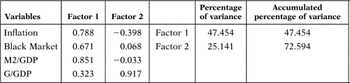
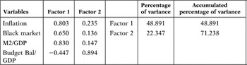
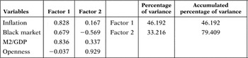
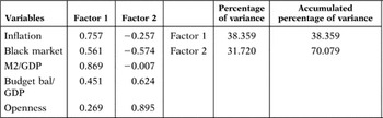
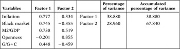
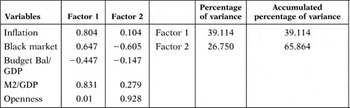
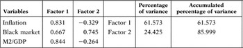
The selection of the variables compounding the IMD is not ad hoc since we have considered those variables that seem more representative of Francoist economic policiesFootnote 16. In the construction of the IMD, we have used factorial analysis based on Principal Component Analysis (PCA hereafter), which assigns weight on the basis of the distributions and interrelations between the various underlining componentsFootnote 17. The results obtained from the application of this methodology are presented in Appendix 2. After exploring different alternative components for the IMD, we reached the conclusion that the «best» index combines three macroeconomic variables: the rate of inflation, the differential between the official and the free market exchange rates (the «black market» premium) and the share of government consumption within total consumptionFootnote 18. Thus, IMD has been obtained as a linear combination of these variables in which the values assigned by PCA to each component, expressed as a proportion of their total value, are used as their respective weight.
The inclusion of these variables can be justified in economic terms. A high (and volatile) rate of inflation implies an absence of sound money and undermines gains from trade, and therefore has a negative impact on economic growthFootnote 19. Moreover, it alters the fundamental terms of long-term contracts, leading to a decrease in economic confidenceFootnote 20.
Exchange rate controls, in so far as they reduce the convertibility of currency, hold back international trade, foreign investment and private confidence in government behaviour. In particular, capital controls do have an important negative effect on economic growth (Chanda Reference Chanda2005). In countries with powerful interest groups, capital controls lead to greater inefficiencies and lower economic growth.
Finally, as regards the share of public consumption in total consumption, it is generally accepted that the government should provide public goods for which free markets do not produce efficient results (De Haan et al. Reference De Haan, Lundström and Sturm2006). However, when public spending increases its share of total spending, political decision-making is substituted for personal choice, and consequently economic freedom declines.
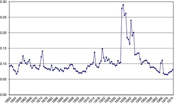
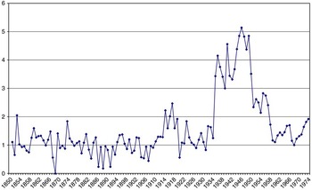
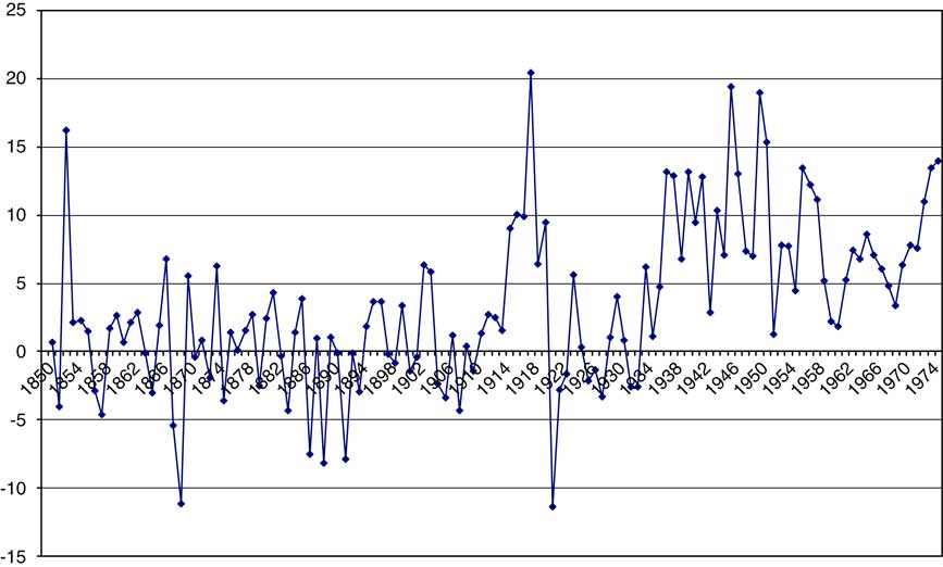
The years 1936-1958 appear to be an exceptional period in the evolution of IMD, with only the milder precedent of the World War I (Figure 6). A significant increase took place from 1936 up to 1947, where it stayed at a high level, until a gradual decline started in 1951, and was sustained during the 1950s. A merely episodic reversal took place between 1956 and 1959, which could be associated with populist policies implemented by the Ministry of Labour, which led to a substantial pay rise across the board in 1956 and a subsequent inflation upsurge (Barciela Reference Barciela2002). Then, the IMD remained stable at low values until it rose again after the 1973 oil shock.
INDEX OF MACROECONOMIC DISTORTIONS 1850-1975
Sources: See Appendix 1 and the text.

4 Assessing the Impact of IMD on Growth: A Structural Model
Per capita income differences across countries are often explained as a result of differences in broad capital endowments and TFP (cf. Hall and Jones Reference Hall and Jones1999). Economic policies under Franco's Regime may have had considerable influence on the sources of economic growth.
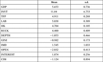
Our starting point is a conventional augmented-Solow model á la Mankiw et al. (Reference Mankiw, Romer and Weil1992), in which GDP (in logs) is dependent on the quantity of labour, in logs, (measured by the number of hours worked, LAB hereafter), the rate of investment (the ratio of gross capital formation to GDP at current prices, INVT), the quality of labour (improvements in labour's skills as a measure of human capital, HK, in logs) and total factor productivity (TFP, in logs)Footnote 21. GDP is not fully defined because we do not include land in our calculations and TFP is not a combination of the INVT, HK and LAB variablesFootnote 22 (Table 2).

SUMMARY STATISTICS

INVT: investment rate; TFP: total factor productivity; LAB: labour quantity; HK: labour quality; RUCK: relative user's cost of capital; IMD: index of macroeconomic distortions; INTEREST: nominal interest rate; CIM: contract-intensive money.
Notes: All the variables are expressed in logs except INVT and IMD.
Sources:
Real GDP, Prados de la Escosura (Reference Prados de la Escosura2003), Table A.11.7.
INVT: Prados de la Escosura (Reference Prados de la Escosura2003), Table A.13.3.
TFP: Prados de la Escosura and Rosés (Reference Prados de la Escosura and Rosés2009).
LAB: Prados de la Escosura and Rosés (Reference Prados de la Escosura and Rosés2009).
HK: Prados de la Escosura and Rosés (Reference Prados de la Escosura and Rosés2009).
RUCK: user's cost of capital, Prados de la Escosura and Rosés (Reference Prados de la Escosura and Rosés2009); GDP deflator: Prados de la Escosura (Reference Prados de la Escosura2003), Table A.11.9.
DEPTH (M2/GDP): M2: Martín Aceña and Pons (Reference Martín Aceña and Pons2005), Table 9.16; GDP, Prados de la Escosura (Reference Prados de la Escosura2003), Table A.13.1.
GINI: Prados de la Escosura (2008).
IMD: see the text.
OPEN (openness measured as % (Exports + Imports)/GDP: Prados de la Escosura (Reference Prados de la Escosura2003), Table A.13.1.
INTEREST: Martín Aceña and Pons (Reference Martín Aceña and Pons2005), Table 9.17.
CIM: (M2-Cash)/M2), Prados de la Escosura estimates (unpublished).
The hypothesis is that macroeconomic distortions, as measured by IMD, decreased efficiency gains and disrupted capital accumulation. For this reason, TFP, HK and INVT have been endogeneised, and thus the impact macroeconomic distortions have on them is taken into account, while allowing for additional exogenous variablesFootnote 23.
There are several channels through which the macroeconomic policy may have affected TFP growth, because this is the result of both efficiency gains and technological changes (Harberger Reference Harberger1998). We postulate that TFP (in logs) depends on IMD, the degree of openness (measured as the ratio of exports plus imports to GDP, OPEN, in logs) and previous levels of human capital and GDP, which are proxies for the actual technological capabilityFootnote 24.

In order to explain investment rates, we have related the share of capital formation in GDP to the relative price of capital, the degree of financial development, the level of GDP and the degree of income inequality. Thus, the rate of capital accumulation has been associated with the relative price of capital goods (Taylor Reference Taylor1998). Here, instead of the relative price of capital goods, we use the user cost of capital, since it is a more accurate measure as it includes the price of capital goods, the interest rate and the depreciation rate, relative to the consumption deflator (hereafter, RUCK). In addition, we expect financial development (measured as M2 over GDP, DEPTH, thereafter) to encourage, ceteris paribus, investment. As regards the role of inequality in capital accumulation, there are competing views: on the one hand, the negative connection between inequality and investment, as a result of social instability, has been stressed (Alesina and Perotti Reference Alesina and Perotti1996); on the other hand, a positive link associating, at low levels of per capita income, inequality with increased saving and investment has been claimed (Kaldor Reference Kaldor1955-1956). We use the Gini coefficient as our income inequality measure (GINI, hereafter). Specifically, the share of investment in GDP (INVT) is related to (the logs of) RUCK, DEPTH, GDP and GINI.

Furthermore, it should be taken into account that price distortions –– caused by factors ranging from taxes on capital goods and barriers to capital goods imports to monopoly rights for domestic capital good producers — play a prominent role in explaining the relative price of capital goods (Jones Reference Jones1994; Collins and Williamson Reference Collins and Williamson2001; Eaton and Kortum Reference Eaton and Kortum2001; Restuccia and Urrutia Reference Restuccia and Urrutia2001). For these reasons, the relative user cost of capital (RUCK) is assumed to depend on IMD and also on GDP level.

Lastly, the quality of labour, or human capital, depends on the level of development (GDP) and past levels of TFPFootnote 25. In the structural model, IMD affects TFP, and TFP affects labour quality.

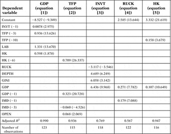
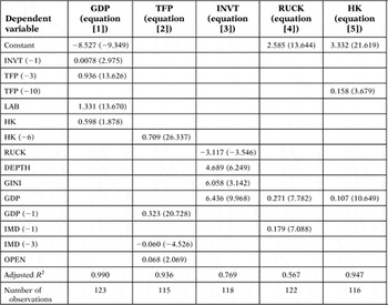
To investigate the relationship between IMD and GDP, we have constructed a structural model as a system of simultaneous equations (equations [1]-[5]) We have used three-stage least squares (3SLS) in the estimate that solves the problem of contemporary correlation between the equations’ residuals and deals with the endogeneity problem often present in this kind of exercise (see Appendix 3 for a detailed exposition of the econometric procedure). The results are presented in Table 3.
ECONOMETRIC MODEL: STRUCTURAL ESTIMATION (1850-1975)
Notes: See Appendix 1 for the definition of independent variables.
Three-stages least square method has been used.
t-ratios are given in brackets; the number of lags appears in brackets after the variable's name. For example INVT (−1).
GDP, TFP, HK, OPEN, LAB and RUCK are in logs. Instrumental variables are:
Equation [1]: constant, INVT (−2), TFP (−2), TFP (−3), LAB (−1), RUCK, IMD, OPEN: OPEN (−1) and OPEN (−2) and HK.
Equation [2]: constant, LAB(−1), HK(−1), GDP (−2), OPEN (−2), OPEN (−3), CIM (−1), CIM (contract-intensive money), [M2−C)/M2], C being currency outside banks (see Clague et al. 1999) and INTEREST (real interest rate).
Equation [3]: constant, INTEREST (−1), INTEREST (−3), IMD: IMD (−1), DEPTH, OPEN (−1), OPEN (−2), GDP (−1) and GDP (−2).
Equation [4]: constant, IMD (−2), IMD (−3), OPEN (−4) and GDP (−1).
Equation [5]: constant, GDP (−1), GDP (−2), TFP (−1), TFP (−2), TFP (−3), IMD: IMD (−1) and OPEN: OPEN (−1).
Sources: Appendix 3.
The results are in line with our predictions, and all variables have the expected sign at the conventional levels of significance. Not surprisingly, we found that IMD had a negative impact on GDP levels channelled through factor accumulation (via the relative price user cost of capital) and TFP levels. The results from equations [2]-[5] help us to establish the relationship between IMD and GDP determinants. Equation [2] shows that a lower degree of macroeconomic distortions, a higher degree of openness and a higher level of human capital and GDP, in previous periods, guarantee a higher TFP level. In fact, a 10 per cent increase in IMD leads to a decrease of about 6 per cent in the TFP level.
Equations [3] and [4] analyse the impact of distortions on physical capital investment. We found that IMD influenced RUCK positively, which in turn influenced investment negatively. In other words, macroeconomic distortions reduced investment by increasing the user cost of capital (note that the partial elasticity of RUCK with respect of IMD is 0.18). Results from equation [3] lend support to the view that attributes lower rates of capital accumulation to higher RUCK. The estimates also suggest that the degree of financial development (DEPTH), inequality (GINI) and the level of GDP are associated with an increase in the rate of investment (INVT). In sum, investment is negatively correlated with distorting policies and positively correlated with inequality and financial development. Why inequality is associated with a higher rate of capital accumulation deserves further research.
Lastly, equation [5] discusses the underlying determinants of human capital levels. No clear-cut evidence of IMD impact on human capital (HK) seems to exist, since it is determined by GDP and TFP levels. However, as discussed earlier, IMD may influence HK indirectly by reducing both TFP and GDP levels.
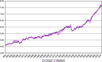
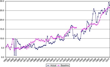
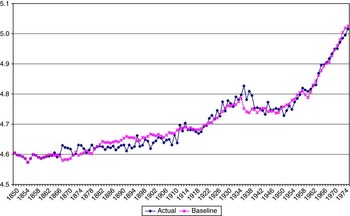
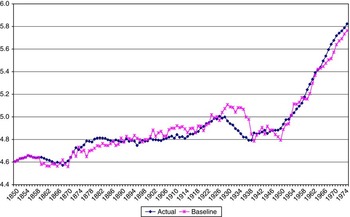
How does the structural model perform? In order to find out we have used its parameters with the historical values of the exogenous variables to predict the value of each dependent variable (GDP, investment, human capital and TFP) and then confront this baseline with its actual value. In Figures 7–10, we observe that the simulated values track the actual values of the endogenous variables reasonably well over the long run and, in particular, during the period considered, 1939-1975, both before and after the 1959 Stabilisation Plan. More specifically, the evolution of GDP and human capital is tracked closely by the model simulations and that of the TFP and the investment rate to a lesser extent. Predictions over shorter periods, however, are less accurate (see, for example, how the model fails to capture the volatility of the actual investment rate and the productivity collapse during the early 1930s).
REAL GDP, 1850-1975 (LOGS): ACTUAL AND MODEL SIMULATION (BASELINE)
Sources: Table 3. See the text.

INVESTMENT RATE (% GDP), 1850-1975: ACTUAL AND MODEL SIMULATION (BASELINE)
Sources: Table 3. See the text.

HUMAN CAPITAL, 1850-1975 (LOGS): ACTUAL AND MODEL SIMULATION (BASELINE)
Sources: Table 3. See the text.

TOTAL FACTOR PRODUCTIVITY, 1850-1975 (LOGS): ACTUAL AND MODEL SIMULATION (BASELINE)
Sources: Table 3. See the text.

In order to estimate the economic impact of macroeconomic distortions, as captured by the IMD, during the early phase of Franco's dictatorship (1939-1959), and thus weigh up the contribution of the 1959 PSL to economic growth, we have carried out a counterfactual exerciseFootnote 26.
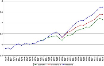
We propose two counterfactual scenarios, in which the estimated coefficients in Table 3 together with the values of each variable may be used to explore some hypothetical alternatives. Firstly, we consider a hypothetical situation in which the average value of IMD during 1939-1951 would have been retained during the period 1952-1975 (scenario I). This is an extreme situation that simulates autarchy throughout the entire Franco regime. Then, a less astringent assumption is made in scenario II: the IMD average value for 1952-1958 would have remained in place until 1975, that is, had the PSL failed to be implemented. This seems a plausible scenario if the reformists’ advice had been rejected by Franco and his closest advisers at the conjuncture of acute lack of foreign reserves faced by Spain in 1959. In scenarios I and II, we expect lower values than those actually observed.
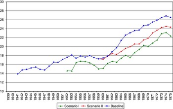
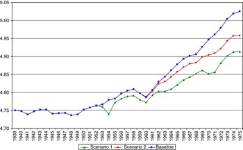
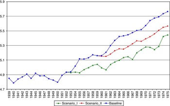
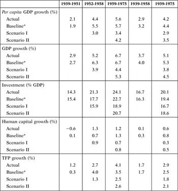
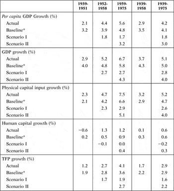
The outcomes of these counterfactual exercises are compared to the baseline results of the structural model for each dependent variable in Figures 11-14, as well as to their baseline and actual values in Table 4. These results lend strong support to the hypothesis that macroeconomic policy conducted during the early part of Franco's regime damaged the Spanish economy severely. For each variable, absolute and per capita GDP, investment, human capital and TFP, the impact of Franco's economic policy was damaging. More prominently, the major channel by which IMD affected economic growth was through TFP. In other words, bad policies translated into lower TFP growth.
REAL GDP, 1939-1975 (LOGS). STRUCTURAL MODEL SIMULATIONS: BASELINE AND COUNTERFACTUAL SCENARIOS
Sources: Table 3. See the text.

INVESTMENT RATE (% GDP), 1939-1975. STRUCTURAL MODEL SIMULATIONS: BASELINE AND COUNTERFACTUAL SCENARIOS
Sources: Table 3. See the text.

HUMAN CAPITAL, 1939-1975 (LOGS). STRUCTURAL MODEL SIMULATIONS: BASELINE AND COUNTERFACTUAL SCENARIOS
Sources: Table 3. See the text.

TOTAL FACTOR PRODUCTIVITY, 1939-1975 (LOGS). STRUCTURAL MODEL SIMULATIONS: BASELINE AND COUNTERFACTUAL SCENARIOS
Sources: Table 3. See the text.

STRUCTURAL MODEL: GROWTH IN ACTUAL AND SIMULATED ECONOMIC POLICY SCENARIOS

TFP: total factor productivity.
Notes:
Scenario I: assumes 1939-1951 IMD (index of macroeconomic distortions) average value was maintained over 1952-1975.
Scenario II: assumes 1952-1958 IMD average value was maintained over 1952-1975.
Sources: Computed with parameters from Table 3. See the text and Appendices 1 and 3.
*Model Simulation.
However, non-negligible differences are observed between the hypothetical results cast by scenarios I and II. To be more precise, for the period 1959-1975, real GDP per head would have grown at 60 per cent of its actual rate under scenario I and at 75 per cent under scenario II.
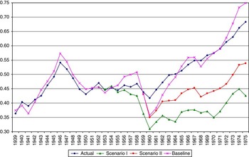
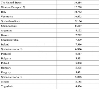
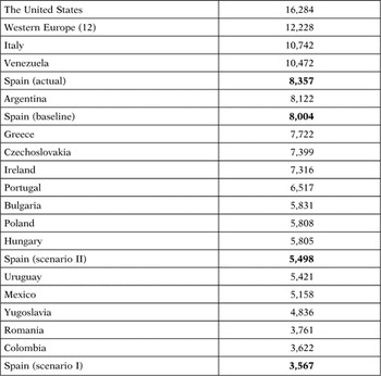
What would have been, then, Spain's relative position at the end of Franco's dictatorship if pre-1959 macroeconomic distortions had remained in place? Spain's counterfactual position relative to Western Europe shows that catching up to Western Europe would have been deferred until the early 1970s under scenario I, and until the mid-1960s under scenario II (Figure 15). Comparative levels of GDP per head in 1975 for actual and counterfactual Spain (resulting from scenarios I and II) are presented in Table 5. Spain, already at the bottom of Western Europe, would have fallen further: below Argentina, Greece and Ireland, and close to Portugal, in the relatively benign scenario II, and below Poland, Hungary and Uruguay, and close to Mexico, in scenario I.
SPAIN'S RELATIVE REAL PER CAPITA GDP, 1939-1975. ACTUAL AND STRUCTURAL MODEL SIMULATIONS (WESTERN EUROPE 12 = 1)
Sources: See Table 5 and the text.

SPAIN'S RELATIVE PER CAPITA GDP IN 1975 (1990 GEARY-KHAMIS $): ACTUAL AND STRUCTURAL MODEL-SIMULATED SCENARIOS

Note: Western Europe (12) is a population-weighted average of Austria, Belgium, Denmark, Finland, France, Germany, Italy, Netherlands, Norway, Sweden, Switzerland and the United Kingdom.
Sources: Spain, Prados de la Escosura (Reference Prados de la Escosura2003) and see text. For other countries, see Maddison (Reference Maddison2010).
To sum up, these counterfactual exercises lend strong support to the hypothesis that macroeconomic policies conducted during the early Franco regime seriously damaged the Spanish economy. Furthermore, the view of the first two decades of Franco's dictatorship (1939-1959) as a monolithic autarchic era is challenged by these resultsFootnote 27. Our results stress that the (de facto) mild and gradual liberalisation that occurred during the 1950s — which translated into lower inflation and a convergence between the official and the free market exchange rate — helped improve economic performance and portrayed the 1959 structural reforms as the response to a growth crisis rather than the reaction to a collapsing economy. As in other historical experiences (i.e. Latin America in the period 1940-1980), in Spain inward-looking policies did not preclude growth but set limits to its sustainability over the long run.
5 Assessing the Impact of IMD on Growth: A VAR Approach
How robust might our results be? In the absence of a theoretical model, a complementary way of assessing the impact of IMD on growth can be obtained through the estimation of vector autoregressive models (VAR), which have the advantage over the previous approach, based on a structural model of not assuming any a priori causal link among the considered variables. At the same time, a VAR approach provides a sensitivity test to the results obtained with the structural model in the previous section.
Our empirical goal is to find a stable long-run relationship between IMD and a set of variables, which constitute the immediate determinants of growth, and to test for causality, that is, for the direction in which these variables influence each other. Owing to the fact that all the variables are integrated of order one (as shown in Appendix 3), we have carried out a stationary VAR analysis between IMD and the relevant variables affecting growth (that is, human and physical capital and TFP), all of them in differences, for the period 1850-1975Footnote 28.
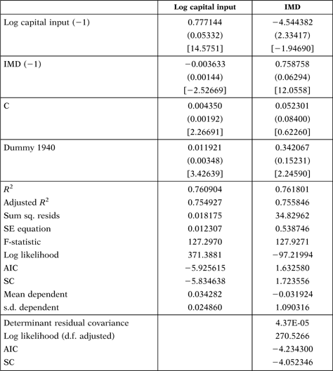
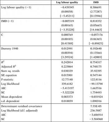
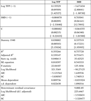
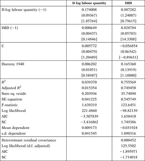
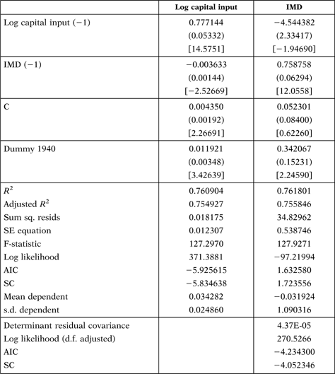
The results are provided in Tables A4.1-A4.4 of Appendix 4. In all cases, IMD is statistically significant. We can observe that the growth rates of physical and human capital and labour quantity, as well as TFP, are negatively affected by IMD. Furthermore, a bidirectional causality between physical capital, on the one hand, and IMD, on the other, has been found. Thus, macroeconomic distortions reduced physical capital accumulation, which in turn led to inefficient policies and new distortions. However, between IMD and human capital, and IMD and TFP, respectively, the causality is unidirectional, and thus macroeconomic distortions result in lower human capital accumulation and efficiency; however, lower growth rates of human capital and TFP do not imply macroeconomic distortions. Our results also confirm a not statistically significant association between IMD and the growth rate of labour quantity.
As with the structural model, we explore two different hypothetical scenarios in an attempt to assess the economic impact of macroeconomic distortions during early Francoism (1939-1959).
Firstly, the individual impact of IMD on broad capital and TFP in scenario I (in which the average value of IMD during 1939-1951 would have remained unaltered for the period 1952-1975) and scenario II (in which IMD average value for 1952-1958 would have been unchanged until 1975) have been estimated. The next step has been to simulate the impact on absolute and per capita GDP of these counterfactual values for labour quantity, broad capital and TFP using the factor shares and the values for land and labour quantity in the Prados de la Escosura and Rosés (Reference Prados de la Escosura and Rosés2009) growth accounting exercise. The results are presented in Table 6, along with the model simulated (baseline) and actual values.
VAR: GROWTH IN ACTUAL AND SIMULATED ECONOMIC POLICY SCENARIOS

VAR: vector autoregression.
Notes:
Scenario I: assumes 1939-1951 IMD average value was maintained over 1952-1975.
Scenario II: assumes 1952-1958 IMD average value was maintained over 1952-1975.
*Model simulation.
Sources: Prados de la Escosura and Rosés (Reference Prados de la Escosura and Rosés2009), Appendix 4 and also see the text.
Our results suggest that, had the macroeconomic distortions of the period 1939-1951 continued throughout the 1950s (scenario I), the growth rate of per capita income would have shrunk to less than half, and that of TFP to two-thirds, while the human capital contribution to growth would have collapsed. The comparison between the outcome of scenarios I and II during the years 1959-1975 allows us to stress the difference the PSL and the subsequent reforms made for Spain's economic performance, while simultaneously underlining the impact of changes in policies and context operated throughout the 1950s. Specifically, under scenarios I and II, per capita income growth would have withered to less than one- and two-thirds, respectively, of the actual figures.
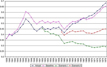
What would have been, then, Spain's relative position at the end of Franco's dictatorship had pre-1959 macroeconomic distortions remained in place? Counterfactual levels of real GDP per head suggest that had pre-1951 economic policies remained in place (scenario I), Spain would have fallen behind Western Europe steadily until 1970, while in the alternative counterfactual hypothesis in which the 1959 PSL would not have been implemented (scenario II), no catching up with Western Europe would have occurred before 1975. The outcome of these simulations shows a deep contrast with the actual (and baseline) catching up taking place between 1959 and 1975, as Spain went up from having less than half of Western European income per head in the 1950s to reaching two-thirds by the time of Franco's death (Figure 16). In Table 7, levels of GDP per head in 1975 for actual and counterfactual Spain are compared with those in OECD, Central and Eastern Europe and Latin America. In these counterfactual simulations, Spain would have fallen behind Portugal, Poland and Hungary in the relatively benign scenario II, and below Romania and Colombia in scenario I. We can conclude, then, that the counterfactual results derived from the VAR approach accentuate those obtained with the structural model.
SPAIN'S RELATIVE PER CAPITA GDP: ACTUAL AND VAR SIMULATIONS, 1939-1975 (WESTERN EUROPE 12 = 1)
Sources: See Table 7 and the text.

SPAIN'S RELATIVE PER CAPITA GDP IN 1975 (1990 GEARY-KHAMIS $): ACTUAL AND VAR-SIMULATED SCENARIOS

VAR: vector autoregression.
Note: Western Europe (12) is a population-weighted average of Austria, Belgium, Denmark, Finland, France, Germany, Italy, Netherlands, Norway, Sweden, Switzerland and the United Kingdom.
Sources: Spain, Prados de la Escosura (Reference Prados de la Escosura2003) and also see text. For other countries, Maddison (Reference Maddison2010).
6 Concluding remarks
This paper has analysed the impact of Franco's economic reforms on Spanish economic growth. The important role played by the new economic policy during the 1950s, particularly the 1959 PSL, in promoting sustained economic growth is confirmed by our results.
A response to an inward-looking growth crisis, the 1959 Stabilisation Plan, gave way to a new institutional set of policies that favoured the allocation of resources along comparative advantage and allowed sustained and faster growth, as well as catching up. Without the PSL, per capita GDP would have been significantly lower at the time of Franco's death, in 1975. However, considerable differences in counterfactual outcomes emerge depending on whether pre-1951 macroeconomic economic distortions had remained in place (i.e. with no economic reforms at all), or whether the 1950s restrictions had been maintained until 1975 (namely, without the PSL being implemented).
Thus, our quantitative results qualify a popular view that depicts the first two decades of Franco's dictatorship as a homogeneous autarchic era and portrays the 1959 PSL as a major discontinuity between two opposite worlds. Without the policy reforms and economic growth of the 1950s, it seems unlikely the PSL would have succeededFootnote 29.
Several suggestions for further research can be extracted from our historical investigation. The advantage of case studies is the first one. Then, in order to analyse historical episodes of major policy reforms, an IMD could be a useful tool. Our investigation also indicates that a detailed analysis of the various channels through which the dictatorship could impact on economic growth seems necessary. Lastly, the experience of Franco's Spain confirms that successful stabilisation programmes can take place under authoritarian political regimes.
Appendix 1: Data sources
«Black market» premium: computed from Martínez Ruiz (Reference Martínez Ruiz2003), Serrano Sanz and Asensio Castillo (Reference Serrano Sanz and Asensio Castillo1997), Reinhart and Rogoff (Reference Reinhart and Rogoff2004), and Martín Aceña and Pons (Reference Martín Aceña and Pons2005), (Table 9.19).
Budget Balance (% GDP): budget balance, Comín and Díaz Fuentes (Reference Comín and Díaz Fuentes2005), (Table 12.24); GDP, Prados de la Escosura (Reference Prados de la Escosura2003)(Table A13.1).
CIM (contract-intensive money): Prados de la Escosura (unpublished estimates).
Financial Depth (M2/GDP): M2, Martín Aceña and Pons (Reference Martín Aceña and Pons2005), Table 9.16; GDP, Prados de la Escosura (Reference Prados de la Escosura2003), Table A13.1.
GINI: Prados de la Escosura (2008).
Government Consumption (% total Consumption) (G/G + C) and (% GDP) (G/GDP): Prados de la Escosura (Reference Prados de la Escosura2003). Table A.13.3.
HK (labour quality): Prados de la Escosura and Rosés (Reference Prados de la Escosura and Rosés2009).
IMD: See the text.
Inflation rate (derived from GDP implicit deflator): Prados de la Escosura (Reference Prados de la Escosura2003), Table A.11.9.
Interest (interest rate): Martín Aceña and Pons (Reference Martín Aceña and Pons2005), Table 9.17.
Investment rate: Prados de la Escosura (Reference Prados de la Escosura2003), Table A.13.3.
K Input (physical capital input): Prados de la Escosura and Rosés (Reference Prados de la Escosura and Rosés2010a).
LAB (labour quantity): Prados de la Escosura and Rosés (Reference Prados de la Escosura and Rosés2009).
OPEN (openness), (exports + imports)/GDP: Prados de la Escosura (Reference Prados de la Escosura2003). table A.13.3.
RUCK (relative user's cost of capital): user's cost of capital, Prados de la Escosura and Rosés (Reference Prados de la Escosura and Rosés2009); GDP deflator, Prados de la Escosura (Reference Prados de la Escosura2003), A11.9.
TFP (total factor productivity): Prados de la Escosura and Rosés (Reference Prados de la Escosura and Rosés2009).
Appendix 2: The Construction of IMD
In this appendix, we will discuss several alternative compositions for our IMD. In order to include variables into the index, we employ Principal Component Analysis. The results are presented in Tables A2.1 to A2.9. The variables considered are: inflation, black market premium, Government consumption (excluding health and education) over total consumption or GDP, budget balance over GDP, M2/GDP, rate of openness and the degree of financial depth (M2/GDP). Although the rationale for including a new variable in the index is that it increases the percentage of the variance explained, we decided to include the variables «black market», inflation and the share of government consumption in total consumption, and not just the first two, because the last one is relevant for the whole considered period, 1850-1975.
IMD 1

IMD: index of macroeconomic distortions.
IMD 2

IMD: index of macroeconomic distortions.
IMD 3

IMD: index of macroeconomic distortions.
IMD 4

IMD: index of macroeconomic distortions.
IMD 5

IMD: index of macroeconomic distortions.
IMD 6

IMD: index of macroeconomic distortions
IMD 7

IMD: index of macroeconomic distortions.
IMD 8

IMD: index of macroeconomic distortions.
IMD 9

IMD: index of macroeconomic distortions.
Sources: Appendix 1.
Appendix 3: Econometrics of the Structural Model
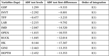
We develop a set of econometric tests over our data before to proceed with estimation of equations [1]-[5] (model of Table 3). Our initial empirical goal is to find a stable long-run relationship between each pair of relevant variables, which will permit us to test for causality. First, we investigate the order of integration of different variables (see Table A3.1).
VARIABLES IN THE STRUCTURAL MODEL: ORDER OF INTEGRATION

ADF: augmented Dickey–Fuller test; INVT: investment rate; TFP: total factor productivity; LAB: labour quantity; RUCK: relative user's cost of capital; IMD: index of macroeconomic distortions; OPEN: openness measured as % (exports + imports)/GDP; HK: labour quality; INTEREST: nominal interest rate; CIM: contract-intensive money.
Notes: All the variables are expressed in logs except INVT and IMD. The ADF test levels have been considered with constant and trend in all cases except for RUCK and IMD that have been considered with only constant and without constant and trend, respectively. The level of significance is in all cases at 1%, except for TFP, which is at 10%.
Sources: See the text.
Owing to the fact that all these variables are integrated of order one, we test the null hypothesis that there is a co-integration relation between IMD and RUCK, RUCK and INVT, IMD and TFP. The results obtained are presented in Table A3.2.
LONG-RUN RELATIONSHIP BETWEEN VARIABLE PAIRS

ADF: augmented Dickey–Fuller test; IMD: index of macroeconomic distortions; RUCK: relative user's cost of capital; TFP: total factor productivity; INVT: investment rate.
Notes: All the variables are expressed in logs except INVT and IMD.
The ADF test levels have been considered with constant and trend in all cases except for the relationship between IMD and TFP that have been considered without constant and without trend. The level of significance is at 5% (**) and at 10% (***).
Sources: See the text.
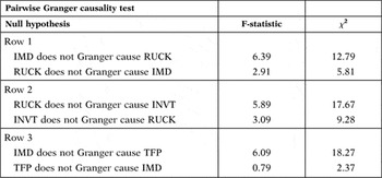
A co-integration relationship has been found between these four pairs of variables, each of these have a common trend, and hence a stable short-run relationship. IMD is affecting positively RUCK, which in turn affects negatively INVT, and negatively to TFP and GDP (as we have predicted earlier). These results lead us to develop a Granger causality test between each variable pair using the residuals from the estimation of the long-run equilibrium relationship.
Granger causality tests of Table A3.3 suggest causality from IMD to RUCK rather than the other way round. Applying a similar approach, we also find that IMD Granger-causes TFP. Therefore, after conducting these co-integration and Granger tests, we are able to confirm that the IMD is behind RUCK and TFP.
GRANGER CAUSALITY BETWEEN IMD, RUCK AND TFP

IMD: index of macroeconomic distortions; RUCK: relative user's cost of capital; TFP: total factor productivity; INVT: investment rate.
Note: The critical values are 2.29 for F-statistic and 11.07 for the χ 2 test.
Sources: See the text.
Appendix 4: Vector Auto Regression Estimates
VAR ESTIMATES BETWEEN PHYSICAL CAPITAL GROWTH AND IMD
VAR: vector autoregression; IMD: index of macroeconomic distortions; Sum sq. resids: sum of square residuals; AIC: Akaike information criteria; SC: Schwarz criteria.
Notes: Data are presented as SE (in parenthesis) and t-statistics [in brackets].
Variables are expressed in differences.
Dummy 1940 is a variable that takes value 0 before 1940 and value 1 after 1940.
Sources: See the text.
VAR ESTIMATES BETWEEN HUMAN CAPITAL GROWTH AND IMD

VAR: vector autoregression; IMD: index of macroeconomic distortions; Sum sq. resides: sum of square residuals; AIC: Akaike information criteria; SC: Schwarz criteria.
Notes: Data are presented as SE (in parenthesis) and t-statistics [in brackets].
Variables are expressed in differences.
Dummy 1940 is a variable that takes value 0 before 1940 and value on1 after 1940.
Sources: See the text.
VAR ESTIMATES BETWEEN TFP GROWTH AND IMD

VAR: vector autoregression; TFP: total factor productivity; IMD: index of macroeconomic distortions; Sum sq. resids: sum of square residuals; AIC: Akaike information criteria; SC: Schwarz criteria.
Notes: Data are presented as SE (in parenthesis) and t-statistics [in brackets].
Variables are expressed in differences.
Dummy 1940 is a variable that takes value 0 before 1940 and value 1 after 1940.
Sources: See the text.
VAR ESTIMATES BETWEEN LABOUR QUANTITY GROWTH AND IMD

VAR: vector autoregression; IMD: index of macroeconomic distortions; Sum sq. resids: sum of square residuals; AIC: Akaike information criteria; SC: Schwarz criteria.
Notes: Data are presented as SE (in parenthesis) and t-statistics [in brackets].
Variables are expressed in differences.
Dummy 1940 is a variable that takes value 0 before 1940 and value 1 after 1940.
Sources: See the text.