Introduction
Since the fourth International Polar Year (IPY 2007–08), the Antarctic Network (ANET) – Polar Earth Observing Network (POLENET) project (2007–12) and the International Gamburtsev Antarctic Mountains Seismic Experiment (GAMSEIS) component of the Antarctica’s Gamburtsev Province (AGAP) IPY project (2007–10) have deployed large numbers of passive seismic stations (POLENET and AGAP stations) in the interiors of West and East Antarctica, respectively. As part of the GAMSEIS project, and under the management of the Chinese Program of Antarctic Nova Disciplines Aspects (PANDA), China has deployed eight seismic stations (CHN stations) along the Chinese Antarctic Research Expedition (CHINARE) traverse between Zhongshan station and Dome A since 2007–08. As more than 97% of Antarctica is covered by ice, most of the inland seismic stations have been deployed on moving ice sheets.
Measuring the motion of the Antarctic ice sheet provides insight into ice dynamics, including the characteristics of the bed. Analysis of seismic data without consideration of ice motion can cause systematic errors because most seismic analysis algorithms assume that the positions of the recording stations are fixed relative to the bed and to each other. For example, a movement of 600 myr-1 will introduce a change of ~0.14 syr-1 in S-wave arrival times using an upper-mantle S-wave velocity of ~4.4 km s-1 in Dziewonski & Anderson (Reference Dziewonski and Anderson1981), which is a significant effect.
The focus of this study was the movement of the seismic stations rather than seismic data. Monitoring the horizontal movement of ice sheets is one of the fundamental goals of Antarctic glaciology. In situ global positioning system (GPS) receivers on the ice can directly measure ice movement (e.g. Budd et al. Reference Budd, Corry and Jacka1982, Manson et al. Reference Manson, Coleman, Morgan and King2000, Zhang et al. Reference Zhang, Dongchen, Wang, Li, Jin and Zhou2008), but observational data regarding inland ice sheet movement are limited because of the harsh conditions and cost of field measurements in Antarctica. One approach to measuring glacial flow rates consists of extracting information on flow patterns from satellite or aerial images taken at known time intervals (e.g. Bindschadler & Scambos Reference Bindschadler and Scambos1991, Testut et al. Reference Testut, Hurd, Coleman, Rémy and Legrésy2003, Cheng et al. Reference Cheng, Li, Shao and Li2007, Rignot et al. Reference Rignot, Mouginot and Scheuchl2011). An ice flow map based on satellite interferometric synthetic aperture radar (InSAR) (Rignot et al. Reference Rignot, Mouginot and Scheuchl2011) shows that ice velocities are >10 m yr-1 in most areas of Antarctica, and greater than 100 m yr-1 on ice shelves and in ice streams.
Velocity determination using satellite images can provide flow measurements over large areas, but this method is less accurate than direct GPS measurement. For example, the nominal precision in the flow speed of the InSAR-based ice velocity map is ~1–17 myr-1 (Rignot et al. Reference Rignot, Mouginot and Scheuchl2011), whereas the horizontal accuracy associated with individual geodetic GPS measurement is <0.1 m giving a velocity error of <0.1 myr-1 for measurements >1 year apart (Zhang et al. Reference Zhang, Dongchen, Wang, Li, Jin and Zhou2008). Greater accuracy is desirable because the majority of the ice in inland Antarctica moves at <10 m yr-1. Furthermore, image analysis normally requires constraints established by previous geodetic ice flow measurements, as well as ground references to typical or stationary topographies or objects (Rignot et al. Reference Rignot, Mouginot and Scheuchl2011). Thus, the InSAR approach may be ineffective in areas where topography is relatively flat, landmarks are absent or flow velocity is low. In some of the regions investigated in this study (areas surrounding three seismic stations: N206, KOLR and WAIS) there are no InSAR data on ice flow rates available (see Fig. 1b; Rignot et al. Reference Rignot, Mouginot and Scheuchl2011). Furthermore, some regions with large lateral velocity variation are not well resolved. Therefore, in situ measurements on these inland ice sheets (e.g. by monitoring the absolute movement speeds and directions at particular locations) are of significant scientific value, and are required to further improve Antarctic ice flow maps.
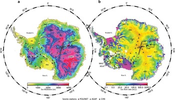
Ice thickness from BEDMAP2 (Fretwell et al. Reference Fretwell, Pritchard and Vaughan2013). b. Ice flow rates (Rignot et al. Reference Rignot, Mouginot and Scheuchl2011). A=Dome Argus, AmH=American Highland, C=Dome Circe, DML=Dronning Maud Land, EANT=East Antarctica, ElL=Ellsworth Land, EnL=Enderby Land, F=Dome Fuji, GSM=Gamburtsev Subglacial Mountains, MBL=Marie Byrd Land, NeS=New Schwabenland, rIS=Ronne Ice Shelf, RIS=Ross Ice Shelf, TAM=Transantarctic Mountains, WANT=West Antarctica.

Seismic stations can operate for multiple years and routinely log their geographical position using stand-alone, navigation-grade, single-frequency GPS receivers. Although data from these receivers are less accurate than those from geodetic GPS, the positions given by single-frequency GPS receivers can still be used to measure ice flow velocity by collecting data over a sufficiently long period of time (van de Wal et al. Reference Van de Wal, Boot, van den Broeke, Smeets, Reijmer, Donker and Oerlemans2008, den Ouden et al. Reference Den Ouden, Reijmer, Pohjola, van de Wal, Oerlemans and Boot2010). Stand-alone, single-frequency GPS units have previously been used to measure ice flow velocities in Greenland (van de Wal et al. Reference Van de Wal, Boot, van den Broeke, Smeets, Reijmer, Donker and Oerlemans2008) and Svalbard (den Ouden et al. Reference Den Ouden, Reijmer, Pohjola, van de Wal, Oerlemans and Boot2010).
In this study, station movement was directly tracked using the geographical position logs of seismic station navigation-grade GPS receivers. The positions logged by seismic stations may provide valuable information on the motion of the ice sheets, especially at locations where no ice flow information is available from satellite imagery. Furthermore, the data may be useful for ground-based verification of satellite ice motion measurements.
Method and data
Global positioning system data logged by seismographs
Global positioning systems provide positioning and timing information based on a constellation of 24 to 32 satellites orbiting the Earth. Each GPS satellite continuously broadcasts information on two frequencies: L1 (1575.42 MHz) and L2 (1227.60 MHz). A GPS receiver calculates its position and the time by precisely timing and analysing the signals transmitted by the GPS satellites (den Ouden et al. Reference Den Ouden, Reijmer, Pohjola, van de Wal, Oerlemans and Boot2010 and references therein).
Global positioning system receivers are routinely incorporated into seismic dataloggers to calibrate the seismograph clock at regular intervals, since seismological measurements require more accurate timing than can be achieved with a stand-alone clock. The GPS time and the geographical position of the seismic station are recorded by the datalogger at regular intervals (usually hourly). Uncertainties in the geographical positioning of several tens of metres are allowable for general seismological investigations, given the precision of travel time observations and the spatial resolution of the studies. Therefore, the horizontal position accuracy of a GPS receiver of several metres, similar to that of a navigation-grade GPS unit (such as those installed in a car), is sufficient for seismic stations.
The Chinese seismic stations deployed in Antarctica (CHN) utilize GURALP dataloggers, which incorporate Trimble Lassen iQ GPS receivers operating on an L1 frequency, C/A code, 12-channel, continuous tracking mode. These receivers have a horizontal position accuracy of <5 m at 50% circular error probable, and <8 m at 90% (Trimble Navigation 2011). Based on this accuracy, the standard deviation (σ) of possible horizontal positions given by the receiver is <6 m, assuming a normal distribution of the position data (50% of data fall within 0.67 σ of the mean, and 90% of the data fall within 1.64 σ of the mean). The CHN stations periodically record instantaneous GPS positions hourly; thus, the recordings in 30 days give a standard error of the mean (SEM) of the horizontal positions of ~0.2 m, based on the positional accuracy of 6 m. The CHN stations only operate during the summer.
The AGAP and POLENET seismic stations use Quanterra Q330 dataloggers, which incorporate i-lotus M12M GPS receivers operating on an L1 frequency, C/A code, 12-channel receiver mode. The position accuracy of the i-lotus M12M GPS receivers is <5 m (1 σ) and <10 m (2 σ) (i-Lotus Corporation Pte 2008). Most AGAP/POLENET stations record GPS information as instantaneous measurements at discrete 1-day intervals, in which case the SEM of horizontal positions over 90 days is ~0.6 m.
Data processing
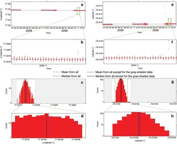
The average ice flow velocity was calculated over the total observation time (mostly ≤3 years) for each station. The GPS positions of a station were separated into given time intervals, ~30 days for CHN stations and ~90 days for AGAP/POLENET stations. For each time interval outliers were removed and the mean position was calculated. Subsequently, the distance between the average position for two different intervals was calculated, and from that the velocity was determined. The process is illustrated in Figs 2 & 3.
GPS positions logged by EAGLE station (position shown in Fig. 1b). a. and e. The original GPS positions. b. and f. Data used to calculate each position. c. and g. Histograms of the data from b. and f., respectively. If the mean is equal to the median, the black line representing the median is covered by the blue line representing the mean.

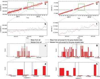
GPS positions logged by UPTW station (position shown in Fig. 1b). a. and e. The original GPS positions. b. and f. Data used to calculate each position. c. and g. Histograms of the data from b. and f., respectively.

Individual GPS positions may occasionally differ significantly from the true position on account of inconsistencies in atmospheric conditions or other complications. The presence of extreme outliers violates the assumption of Gaussian statistics and will bias estimates of the mean and standard deviation. To remove outliers in a time interval (e.g. ith interval), the averaged position (
 $$\bar \phi $$
(i),
 $$\bar {\lambda}$$
(i)) (represented by
 $$\bar {x}$$
(i)) and standard deviation (σ
ϕ
(i), σ
λ
(i)) of the latitudinal (ϕ) and longitudinal (λ) positions were first calculated over the interval. The GPS position distribution is close to a normal or uniform distribution. Generally, 98.8% of data satisfying a normal distribution will be within a distance of ~2.5 σ from the mean of the data, and all data that are uniformly distributed in the range (–c, c) will be within a distance of 2 σ because the standard deviation (σ) of the data is equal to 0.577c; therefore, most reliable data should be within a distance of ±2.5 σ from the mean. The GPS positions with a distance of ≥2.5 σ
ϕ
(i) in latitude or ≥2.5 σ
λ
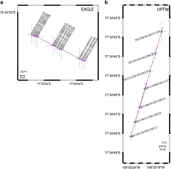
(i) in longitude from the respective mean (e.g. areas shaded grey in Figs 2c & 3c) were discarded. On average, the number of remaining GPS positions within each time interval was 735±235 for CHN stations and 89±7 for AGAP/POLENET stations. Using the positions after outliers were removed, the position mean and standard deviation was calculated again. The location variations of the two example stations in Figs 2 & 3 over several different time intervals are shown in Fig. 4.
Movement of seismic stations a. EAGLE and b. UPTW. Each point represents the average GPS position during a given time interval; the standard error of the average GPS location is indicated by a blue error bar; the standard error of the GPS observations is indicated by a grey error bar; the start/end dates of the GPS monitoring periods for each average GPS location are labelled. The pink arrows show glacier movement rates calculated from only two successive positions.

The great-circle distance and azimuth between the average position (
 $$\bar {x}$$
(i) and
 $$\bar {x}$$
(i+1)) in the two successive ith and (i+1)th intervals were then calculated, from which the displacement (d
ϕ
(i,i+1), d
λ
(i,i+1)) between the two intervals was obtained. The movement velocity v(i,i+1) during the two intervals was calculated by dividing the displacement by the time difference Δt(i,i+1) between the average times (t(i) and t(i+1)) of the data within ith and (i+1)th intervals, respectively. The magnitude of station movement during successive time intervals, such as that for station EAGLE (Fig. 4a), may vary slightly from one time interval to the next. The variations can result from errors in the GPS data, or from temporal variations in the velocity of the ice.
There were a few cases in the data of sudden large movements, which generally corresponded to times of known station servicing and redeployment. Velocity outliers that deviated by >1.5 σv (σv represents the standard deviation of all the velocities at a station) were removed from the mean based on the same rationale as the removal of position outliers. Finally, the velocity mean (
 $$\bar{v}_{\phi } ,\,\bar{v}_{\lambda } $$
) (represented by
 $$\bar{v}$$
) was calculated from all the velocities at each seismic station. The average velocity
 $$\vec {v}$$
during the full observation time was also calculated using only the records in the first and last (nth) intervals, i.e. by dividing the displacement (d
ϕ
(1,n), d
λ
(1,n)) by the time difference Δt(1,n). The removal of velocity outliers eliminates the effect of sudden large variations in station positions in the calculation of the velocity mean (
 $$\bar{v}$$
) but not of the average velocity (
 $$\vec {v}$$
).
Velocity uncertainty
The resulting velocity estimates include fixed seismic stations, installed on a rock base or in stationary snow near a nunatak rather than on flowing ice that would not be expected to have significant motion. These sites serve as an additional test of the method to illustrate the measurement accuracy of the GPS receivers. The Antarctic plate moves at a rate of <0.1 m yr-1 in the ITRF 97 frame (e.g. Bouin & Vigny Reference Bouin and Vigny2000), thus the movement of a fixed AGAP/POLENET station, such as LONW at Lonewolf Nunatak, can be discounted because the rate is smaller than the SEM of all the 1-year GPS positions of a AGAP/POLENET station of ~0.3 m. The GPS position measurements over a long period of time follow a normal distribution, which can be indicated from a quantile-quantile (QQ) plot of 5-year recordings from the LONW station (Fig. S1 found at http://dx.doi.org/10.1017/S0954102014000704), and for most (>90%, <1.68 σ) of the data (~90 positions) in 3 months (Fig. S1). The position accuracy of a fixed station can be taken as the upper limit of the accuracy of the GPS position of a station deployed on ice, and the estimated velocity can be taken as the upper accuracy limit of velocity at a station on ice.
For a station deployed on rapidly moving ice, such as an ice stream, the ice velocity may be large enough that the distribution of horizontal GPS positions of the station will be non-Gaussian and may even approach a uniform distribution over a longer period of time. For example, the distribution of 2-year GPS positions of the UPTW station, deployed on Thwaites Glacier (75°30'S, 106°45'W, West Antarctica), where the ice moves with a velocity of ~117 m yr-1, is close to uniform, as shown by the QQ plot in Fig. S2 (found at http://dx.doi.org/10.1017/S0954102014000704). However, during a short time interval, i.e. a period during which the ice displacement is smaller than the accuracy of the GPS, the distribution is still close to normal, as shown in Fig. S2 for UPTW.
If all GPS positions in the ith time interval are consistent with either a normal or uniform distribution, the mean
 $$\bar x$$
(i) is equal to the median, and represents the position x(i) at the average time t(i) of the data within the interval. The accuracy of x(i) is less than the SEM of all the GPS positions if the station moves; that is, the SEM of the real position is the lower limit of the accuracy of x(i). Even though the distribution of GPS positions from the ice surface, such as the latitudes of the UPTW station, shows some departure from both normal and uniform distributions, the difference between the mean and median of 90-day interval latitude measurements (~7×10⁻⁶°=~0.77 m) (see Fig. 3g & h) is much smaller than the displacement (~29 m) during that same time interval (90 days).
Given standard deviation σx as the accuracy for all x(i), the accuracy in the distance between two positions, or the accuracy in the displacement between the two intervals, is ~1.4 σx according to error propagation. If the time difference Δt(i,i+1) is 1 month and Δt(1,n) is 1 year, the accuracy (or uncertainty) in v(i,i+1) is ~1.4×12 σx m yr-1, in
 $$\vec {v}$$
is ~1.4 σx m yr-1, and in the mean (
 $$\bar{v}$$
) from 12 velocities is
 $\,\sim\!{\rm 1}.{\rm 4}{\times}{\rm 12}/\sqrt {12} $
σx m yr-1. For the GPS position logged by a CHN seismic station, the positions are separated at 30-day intervals, thus Δt(i,i+1) is 30 days and the accuracy in the displacement during two successive time intervals is 0.28 m, based on error propagation from the same accuracy of 0.2 m in each of the two average positions. Therefore, the accuracy (or uncertainty) in v(i,i+1) is 3.4 (= 0.28×365/30) m yr-1, in
 $$\vec {v}$$
when Δt(1,n) is 1 year is ~0.28 m yr-1, and in
 $$\bar{v}$$
from the 12 velocities is 1.0 (
 $${\rm =3}.{\rm 4}/\sqrt {12} $$
) m yr-1. The GPS positions of AGAP/POLENET stations are separated at 90-day intervals, thus Δt(i,i+1) is 90 days and the accuracy in displacement is 0.8 m, based on an error of 0.6 m in each of the two positions. If Δt(1,n) is 1 year, the accuracy in v(i,i+1) is 3.2 (=0.8×365/90) m yr-1, in
 $$\vec {v}$$
is 0.8 m yr-1, and in
 $$\bar{v}$$
from four velocities in 1 year is 1.6 (
 ${\rm =3}.{\rm 2}/\sqrt 4 $
) m yr-1.
In the above estimation, some uncertainties are not considered. If the longitude and latitude distributions are normally distributed and independent, the geographical positions (and then the displacement) given by a GPS receiver can be more similar to a Rayleigh distribution than to a bivariate normal distribution, and the error propagation is more complex (Zandbergen Reference Zandbergen2008). Furthermore, the true velocity of the ice at a station may be non-uniform during a given interval. Instantaneous accelerations or decelerations during a time shorter than the interval of interest cannot be resolved because only data on the mean during each time interval are used. However, the difference between the mean during a time interval and the true position at the average time of the interval is not more than half the value of the displacement during the interval.
Results
The
 $$\bar{v}$$
and
 $$\vec {v}$$
at each station for the full observation time are shown in Table S1 (found at http://dx.doi.org/10.1017/S0954102014000704).
If the GPS antenna of a station is fixed on the ice during the full observation time, the difference between
 $$\bar{v}$$
and
 $$\vec {v}$$
should be smaller than the velocity uncertainty. Sudden variations in station position between two neighbouring time intervals can be removed as outliers in our calculation of
 $$\bar{v}$$
but not
 $$\vec {v}$$
thus a large difference between the two velocities indicates that a sudden long-distance movement occurred. A large difference (>35 m yr-1) between
 $$\bar{v}$$
and
 $$\vec {v}$$
was found for the AGO1 and N140 stations (Table S1). The original GPS positions show that N140 moved 292 m on 27 December 2009 and AGO1 moved 207 m on 29 December 2009, these movements correspond to station redeployments recorded in the station records. The GPS antenna of the P061, DNTW and WAIS stations were also moved a short distance (>10 m) during field servicing, indicating that the velocity outliers were not the result of ice flow acceleration. For DT154, a small number of valid continuous GPS positions in one time interval in October 2009 resulted in a large uncertainty. In order to remove the error in the velocity calculation resulting from servicing or redeployment, or large position uncertainty in a time interval, a separate calculation of
 $$\bar{v}$$
and
 $$\vec {v}$$
before and after the period of the outlier was made for each station, thereby providing a better estimate of ice flow. These corrected results are given in Table I.
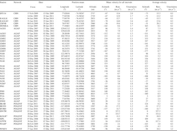
Velocity of ice flow at seismic stations.

* No ice flow data available from InSAR-based measurements.
For all fixed stations, on rock outcrops or stationary snow,
 $$\bar{v}$$
was 0.37±0.24 m yr-1 (Table S1), representing upper limit of accuracy in velocity. The small velocities obtained for the fixed stations are consistent with the estimated uncertainty of 0.2–0.5 myr-1 (Table I). The uncertainty for the estimated average velocities for all the other stations was ~0.3–1 m yr-1 (Table I).
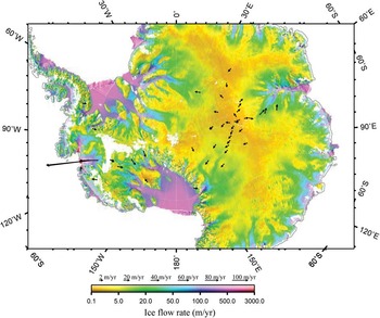
The ice flow velocity at all the stations on ice are shown in Fig. 5. Two of the POLENET stations (UPTW and DNTW) deployed on Thwaites Glacier recorded velocities of >100 myr-1 (117 and 332 myr-1, respectively; see Table I and Fig. 5). Due to the rapid movement the true uncertainty associated with the positions of these stations (relative to a fixed station) are larger than shown in Table I. In regions with rapid ice flow, if calculated relative to a fixed station, the >100 m change in the position of the station will introduce systematic errors into seismic analysis results. Thus, using a time-varying station position is recommended to reduce the errors associated with seismic sensor positions.
Ice flow velocities across Antarctica. Colours denote the ice flow rates (Rignot et al. Reference Rignot, Mouginot and Scheuchl2011). Arrows represent the average velocities show in Table I.

Discussions
Comparison with geodetic global positioning system measurements
Lambert Glacier, East Antarctica, is the largest glacier in the world (http://nsidc.org/data/radarsat/gallery/lambert_mapw.html). The ice flow rates at Lambert Glacier and Amery Ice Shelf have been obtained using high-accuracy geodetic GPS measurements (e.g. Budd et al.
Reference Budd, Corry and Jacka1982, Manson et al.
Reference Manson, Coleman, Morgan and King2000, Kiernan Reference Kiernan2001, Ren et al.
Reference Ren, Allison, Xiao and Qin2002, Zhang et al.
Reference Zhang, Dongchen, Wang, Li, Jin and Zhou2008). Four of the seismic stations (DT154, CHNB, EAGLE/EAGLE2 and DOMEA) are close to positions used for the geodetic measurements by Zhang et al. (Reference Zhang, Dongchen, Wang, Li, Jin and Zhou2008). Our results were compared with those of geodetic GPS measurements and velocities (
 $$\hat{v}$$
) from InSAR-based images (Fig. 6a). Ice velocity (
 $$\tilde{v}$$
) was estimated at DT154 and CHNB by linear interpolation from two neighbouring geodetic measurements which are located within 10–50 km from the stations. However, non-linear variation in ice flow velocity between the geodetic measurements cannot be resolved in the interpolation.
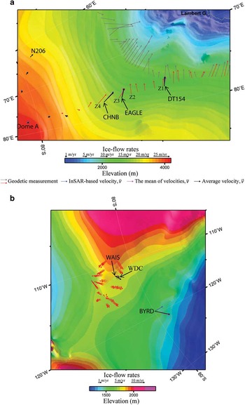
Ice flow velocities a. along the traverse from Zhongshan to Dome A and b. in West Antarctic Ice Sheet (WAIS) divide (region positions are marked by dashed rectangles in Fig. 1b). Colours denote surface topography from ETOPO2. Mean velocities and average velocities are shown in Table I. The InSAR-based velocities are from Rignot et al. (Reference Rignot, Mouginot and Scheuchl2011). The geodetic measurements are from a. Kiernan (Reference Kiernan2001) (grey arrows) and Zhang et al. (Reference Zhang, Dongchen, Wang, Li, Jin and Zhou2008) (red arrows) and b. Matsuoka et al. (Reference Matsuoka, Rasmussen and Power2011). The circle labelled with ‘WDC’ marks the position of the WAIS divide ice core.

At DT154 station
 $$\vec {v}$$
(Fig. 6a black arrows) is slightly different from
 $$\bar{v}$$
. The velocity vectors
 $$\vec {v}$$
and
 $$\hat{v}$$
(Fig. 6a blue arrows) are similar to one another, and they closely parallel the nearby geodetic measurements (Fig. 6a red arrows; Zang et al. 2008) (e.g. Z1 in Fig. 6a). The speed of
 $$\vec {v}$$
(13.2 m yr-1 at an azimuth of -71°) is ~10% greater than
 $$\tilde{v}$$
(11.9 m yr-1 at an azimuth of -70°), and the azimuth difference (1°) of the two velocities is negligible.
EAGLE station was re-installed on 31 January 2010 at a distance of ~10 m from its original position and was renamed EAGLE2 (Table I). At EAGLE,
 $$\vec {v}$$
is similar to, and nearly overlaps,
 $$\bar{v}$$
and
 $$\hat{v}$$
(Fig. 6a, Table I). The value of
 $$\vec {v}$$
at EAGLE2 is nearly the same as that of EAGLE, although
 $$\vec {v}$$
of EAGLE2 varies slightly from
 $$\bar{v}$$
. The large uncertainty in
 $$\bar{v}$$
at EAGLE2 is a result of the short duration of data acquisition at this site. A comparison of ice sheet movement at EAGLE/EAGLE2 with the geodetic measurements at positions Z2 and Z3 (Fig. 6a) shows small differences in movement direction. The differences indicate that the ice movement close to the EAGLE/EAGLE2 station is spatially quite variable, which may be related to the position of the station on an inflection point of both ice thickness contours (Fig. 1a) and topographical contours (Fig. 6a), which causes considerable variation in the direction of the steepest downslope vector as compared with vector directions in nearby areas.
For station CHNB, all velocities (
 $$\vec {v}$$
,
 $$\bar{v}$$
and
 $$\hat{v}$$
) were similar, and are roughly the same as those indicated by nearby geodetic measurements at the positions labelled Z3 and Z4 (Fig. 6a; Zhang et al.
Reference Zhang, Dongchen, Wang, Li, Jin and Zhou2008). The speed of
 $$\vec {v}$$
(20.3 m yr-1 at an azimuth of -31°) is ~12% greater than
 $$\hat{v}$$
(18.1 m yr-1 at an azimuth of -35°), and the azimuth difference (4°) of the two velocities is small.
At the station on Dome A, the ice movement is very slow, thus the velocity is not bigger than the measurement error (Table I).
In West Antarctica, a deep ice-coring project on the West Antarctic Ice Sheet (WAIS) divide has been conducted (Fudge et al. Reference Fudge, Steig and Markle2013), in which ice flow velocities were measured by geodetic GPS during two consecutive field seasons in 2005–06 and 2006–07 (Matsuoka et al. Reference Matsuoka, Rasmussen and Power2011). The WAIS seismic station is located several kilometres from the sites of the geodetic GPS measurements (Fig. 6b). The geodetic measurements show that both the ice-surface topography contour and the ice flow directions vary significantly over short distances in this area. The ice flow azimuths at WAIS and BYRD stations are nearly perpendicular to the ice-surface topographical contour, along the direction of the steepest downhill vector. The geodetic measurements are distributed on the two sides of the topographical ridge, and most of the measured ice flows are generally along a downhill direction. However, parts of the measured velocities show a small angle with the ice-surface topographical contour, suggesting that the topographical data of ETOPO2 used here may not be enough to represent the variation of the local topography; the spatial resolution length (~4 km) in ETOPO2 may be longer than the extent of the variation of the local topography. The ice flow speed calculated from the GPS of the WAIS seismic station is similar to the nearby geodetic measurements.
In total, the ice velocities obtained in this study from GPS data at stations DT154, CHNB, EAGLE/EAGLE2 and WAIS, especially the values for
 $$\vec {v}$$
, are similar to and consistent with those obtained using geodetic measurements. Therefore, results obtained using navigation-grade GPS measurements reliably represent ice flow velocities at seismic station locations, demonstrating that these data are useful not only for analyses of the seismic data, but also to constrain ice movements. The errors in
 $$\vec {v}$$
are smaller than the errors in
 $$\bar{v}$$
at all stations; therefore, the velocities given by
 $$\vec {v}$$
are the most accurate representation of ice movement.
Comparison with InSAR-based velocities
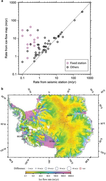
Figure 7a shows the comparison of velocities obtained from the InSAR-based ice flow map (
 $$\hat{v}$$
) with
 $$\vec {v}$$
and
 $$\bar{v}$$
. Figure 7b shows the distribution of the differences between
 $$\hat{v}$$
and
 $$\vec {v}$$
. The uncertainties for ice velocities obtained from InSAR-based images are ~1–17 m yr-1 (Rignot et al.
Reference Rignot, Mouginot and Scheuchl2011), which are larger than the uncertainties in this study (~0.3−1 m yr-1). Ice flow velocity data from InSAR (Rignot et al.
Reference Rignot, Mouginot and Scheuchl2011) are not available for the positions of the N206, KOLR and WAIS stations (Fig. 7b); moreover, data for a large area of West Antarctica is not available (Fig. 7b). The WAIS and KOLR stations move with a velocity of ~3 m yr-1 and 10.9 m yr-1, respectively (Fig. 5, Table I). The ice at N206 station moves with a velocity of ~3.8 m yr-1 (Figs 5 & 6, Table I).
Comparison of ice flow rates obtained from InSAR (Rignot et al. Reference Rignot, Mouginot and Scheuchl2011) and those obtained from the GPS positions of seismic stations. a. The black circles indicate the average velocity (Table I), and the pink circles indicate the mean velocity of fixed stations (Table S1 found at http://dx.doi.org/10.1017/S0954102014000704). b. The blue circle shows the difference between the data at each station, and red squares mark the positions where the difference cannot be calculated because no ice flow velocity from InSAR was available.

When the ice velocity measured by the navigation-grade GPS at the seismic station is >2 m yr-1, these velocities are close to those obtained by InSAR (Fig. 7a). However, at sites with low velocity (<2 m yr-1), large differences (even >10 m yr-1) between the two approaches can be found. The velocities of <2 m yr-1 are close to the accuracy (~0.3–1 m yr-1) in this study and the upper limit of the accuracy for InSAR-based measurements; therefore, all the results may include relatively large uncertainty. However, the difference is generally larger than the accuracy in our results and also that given in the InSAR-based study (Rignot et al. Reference Rignot, Mouginot and Scheuchl2011). The geographical distribution of the differences (Fig. 7b) shows that all the locations with a difference of >10 m yr-1 between the two datasets are close to or on an ice stream (e.g. DEVL, UPTW, DNTW), or close to a fixed station (Fig. 7a). These areas have complex lateral gradient in ice movement velocities, indicating that the discrepancies may be due to large local lateral gradients. For example, the InSAR-based ice flow velocity at the position of a fixed station can be as large as ~40 myr-1 (Fig. 7a). Almost all of the discrepancies show the velocity measured by the seismic station is much less than the velocity measured by InSAR, suggesting that many of these stations are deployed in regions of slow moving ice at the edge of ice streams and regions of larger ice velocity. For a region with large lateral velocity variation, spatial resolution length becomes very important to evaluate the model for a geo-scientific study (An Reference An2012).
Comparison with ice surface downhill directions
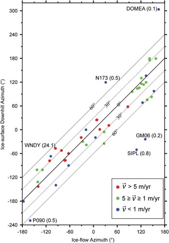
Glaciers flow downhill due to gravity and the internal deformation of ice in the direction of the surface slope (Greve & Blatter Reference Greve and Blatter2009, Cuffey & Paterson Reference Cuffey and Paterson2010). Our determined ice velocity vectors shown in Fig. 6 are generally perpendicular to the ice-surface topography contour or along the steepest downhill direction as expected. Additionally, the steepest downhill azimuth was calculated at each of the seismic stations from the topographical data of ETOPO2, its relationship with the ice flow azimuth at the station is shown in Fig. 8. A positive azimuth is an angle measured clockwise from north and a negative azimuth is anticlockwise. The differences between the two azimuths for five stations (DOMEA, N173, GM06, SIPL and P090) are >65°, which may be due to low reliability of the ice velocities for these slowly moving stations. The uncertainty in direction of flow becomes very large for stations moving close to the accuracy of the measurement; the velocities of each outlier station (Fig. 8) are smaller or close to the accuracy (~0.3–1 m yr-1) in our estimation. The ice velocities of WNDY station (Fig. 8) are large and more reliable; however, the difference (~50°) between the two azimuths of the station is relatively large, which may be due to ice flow not following the topography or the topographical data of ETOPO2 having a low spatial resolution (~4 km) and cannot show complex horizontal topographical variation. In any case, the difference for 70% of all velocities of >1 m yr-1 is <28°, indicating the ice flow azimuths generally follow downhill directions and confirming the reliability of our results.
The relationship between ice flow azimuth and ice surface steepest downhill azimuth at all seismic stations over ice. The ice flow azimuths are of the mean velocities (Table I); and the steepest downhill vector are calculated from ETOPO2. The label such as ‘DOMEA(0.1)’ represent station name and ice flow mean velocity in m yr-1. The lines represent iso-contours of differences between ice flow and ice surface downhill azimuths.

Conclusions
Since the fourth IPY in 2007–08, the international community has deployed passive seismic stations over much of the Antarctic ice sheet as part of the GAMSEIS-AGAP and ANET-POLENET projects. Using the longitudinal and latitudinal positions given by navigation-grade GPS receivers in the seismic stations, the station positions were tracked as they moved with the underlying ice sheet. Generally, ice velocities are sufficiently fast that rates of ice movement estimated by navigation-grade GPS are consistent with those obtained by measurements made at nearby sites by high-accuracy geodetic GPS, including three seismic stations along the CHINARE traverse from Zhongshan station to Dome A in East Antarctica and at a station at the WAIS divide. Most of the estimated velocities move in a direction within 28° of the steepest downhill vector of the ice surface slope. The consistencies indicate that our position variation data are useful for analyses of the seismic data, and the ice flow velocities estimated from the stations can also help constrain Antarctic ice sheet movement with a velocity of ≥1 m yr-1, particularly in regions with limited previous geodetic GPS monitoring (e.g. the broad intra-continental regions of Antarctica) or with a large lateral gradient in ice velocities (e.g. West Antarctica). The uncertainty of navigation-grade GPS measurements (~0.3–1 m yr-1) is smaller than the error of ice velocity maps obtained from satellite images (~1–17 myr-1); therefore, our data are useful for constraining ice flow map data obtained from satellite images and providing ground-truth data to confirm and refine these measurements. In addition, the seismic stations have provided unique ice sheet velocity data for three locations where no ice flow information is available from InSAR data.
Acknowledgements
All Chinese field work was conducted by the 24th–27th Chinese National Antarctic Research Expeditions during 2007–11, and the fieldwork at the seismic stations during the 24th expedition (2007–08) was conducted by Dr Xiao Cheng. We are grateful for the logistical support of the Antarctic Administration of China and all members of the Chinese inland icecap expeditions. The US GAMSEIS-AGAP and ANET-POLENET stations were deployed with the assistance of the IRIS/PASSCAL instrument center. The criticisms and detailed comments from Editor Laurie Padman and three anonymous reviewers were very helpful for the improvement of the text. This work was funded by the National Natural Science Foundation of China (grant No. NSFC-40874021), Chinese Polar Environment Comprehensive Investigation & Assessment Programmes (grant No. CHINARE2013-02-05), the Chinese PANDA in the IPY, and US National Science Foundation (grants ANT-0537597 and ANT-0632209). All figures are generated using the Generic Mapping Tools (GMT) (Wessel & Smith Reference Wessel and Smith1991).
Supplemental material
Supplemental figures and a table will be found at http://dx.doi.org/10.1017/S0954102014000704.