3.1. Rough-surface drag and pressure

For rough surfaces characterised by varying statistical properties, the primary flow characteristic of interest is the friction resistance, as depicted in figure 3. The friction resistance coefficient and pressure resistance coefficient of the rough surface can be determined through the following equations (Jelly et al. Reference Jelly, Ramani, Nugroho, Hutchins and Busse2022) $\colon$

(3.1) \begin{align} {{C}_{\textit{fi}}}=\frac {\mu \left ( \dfrac {\partial {{U}_{i}}}{\partial {{x}_{\!j}}}+\dfrac {\partial {{U}_{\!j}}}{\partial {{x}_{i}}} \right )}{\dfrac {\rho U_{\infty }^{2}}{2}}\dfrac {\dfrac {\partial F}{\partial {{x}_{\!j}}}}{\left \| \dfrac {\partial F}{\partial {{x}_{\!j}}} \right \|}, \text{ }{{C}_{p}}=\dfrac {\left ( P-{{P}_{0}} \right )}{\dfrac {\rho U_{\infty }^{2}}{2}}\frac {\dfrac {\partial F}{\partial {{x}_{\!j}}}}{\left \| \dfrac {\partial F}{\partial {{x}_{\!j}}} \right \|},\\[-10pt]\nonumber\end{align}

(3.2) \begin{align} F\left ( x,y,z \right ) &=h\left ( x,z \right )-h=0,\end{align}

where $\mu$ is dynamic viscosity, $h(x, z)$ is rough surface height function, $h$ is rough surface height equal to $y$ when the surface is placed on a flat plate, $F ( x,y,z )$ stands for the equation of the rough surface, subscripts $i,j$ follow the Einstein summation convention, ${P}_{0}$ is the inlet pressure, ${U}_{i}$ is the time-averaged velocity.

Figure 3.

(a) The distribution of streamwise friction coefficients for the nine rough surfaces is presented, with the isosurface only showing the parts of forward flow. (b) An overview of the streamwise friction resistance coefficient ${C}_{\textit{fx}}$ isosurfaces for negative skewness group (red) and positive skewness group (blue) is depicted, with the higher area highlighted by green isolines.

Figure 3(a) shows the streamwise friction coefficient distribution in each case. It can be found that the streamwise resistance of c_1_0 is distributed evenly, and the streamwise resistances of the ${E{{S}_{z}}}/{E{{S}_{x}}}=0.52$ group are concentrated in the structure with a certain streamwise wavelength modulated by small $E{{S}_{z}}/E{{S}_{x}}$ . Relatively, the resistances of the ${E{{S}_{z}}}/{E{{S}_{x}}}=2.40$ group are concentrated at the spanwise crest. Comparative analysis of cases under identical ${E{{S}_{z}}}/{E{{S}_{x}}}$ reveals that the area of peak resistance, induced by negative skewness, is substantially expanded. This is attributable to the presence of several large-scale, profound indentations that create an increased number of elevated regions, which are the primary locations of resistance distribution. As can be seen from table 2, structures modulated along the spanwise direction by large $E{{S}_{z}}/E{{S}_{x}}$ will generate greater streamwise resistance with the same skewness. For the remaining cases with significant positive and negative skewness, as described in §2.1, they are obtained by inverting each other’s y-coordinates, i.e. their peaks and pits correspond to each other. Therefore, it can be clearly shown in figure 3(b) that irrespective of $E{{S}_{z}}/E{{S}_{x}}$ , under positive skewness, streamwise resistance is primarily concentrated in the vicinity of rough peaks, whereas in negative skewness, it bypasses the depressed regions, aggregating in the elevated zones external to these depressions. Table 2 indicates that, with the same $E{{S}_{z}}/E{{S}_{x}}$ , the integrated-averaged value of streamwise resistance is consistently maximised in negative skewness, which aligns with the larger resistance peak area attributed to negative skewness as depicted in figure 3(a). This finding contradicts the consensus from prior research suggesting that positive skewness friction resistance exceeds that of negative skewness (Yang et al. Reference Yang, Stroh, Chung and Forooghi2022; Busse & Jelly Reference Busse and Jelly2023). They postulate that the increased recirculation zones under negative skewness counteract some of the surface forces imposed by the forward flow. However, in the presence of sparsely distributed large-scale depressions in the negative skewness cases, the generated recirculation is insufficient to offset the augmented resistance resulting from the expanded high-altitude zones. Consequently, the overall resistance exceeds that observed under positive skewness.

Table 2.

Integrated-averaged values of the streamwise friction coefficient $({\widehat {C}}_{\textit{fx}})$  on the rough surfaces.

Figure 4.

(a) Distribution of pressure coefficients for the nine rough surfaces. (b,c) The negative and positive ${C}_{px}$ components of cases of negative skewness and positive skewness are examined, with the higher area highlighted by green isolines.

The pressure resistance is intricately linked to the friction resistance. Figure 4(a) presents the distribution of the pressure coefficients for each rough surface. Positive values typically correspond to the windward face, whereas negative values denote the leeward side. The isosurfaces of figure 4(a) fit well with the height distributions of figure 1. It is worth noting that in the $E{{S}_{z}}/E{{S}_{x}}=2.40$ group, the structure, significantly influenced by large $E{{S}_{z}}/E{{S}_{x}}$ values, lacks a consistent spanwise wavelength; the grooves oriented along the streamwise direction do not extend across the entire rough surface. For cases of negative skewness and positive skewness, figures 4(b) and 4(c) elucidate their distinctive characteristics $\colon$ the negative pressure coefficients are concentrated downstream of the rough peaks under positive skewness and upstream of the pits under negative skewness, while the positive pressure coefficients exhibit the opposite pattern. This indicates the formation of local recirculation zones within each pit. The correlation coefficients for the ${C}_{px}$ distribution of cases of negative skewness and positive skewness under identical $E{{S}_{z}}/E{{S}_{x}}$ are computed, as defined hereafter $\colon$

(3.3) \begin{equation} {{\sigma }^{*}}_{A,B}=\frac {\textrm{cov}\left ( A,B \right )}{{{\sigma }_{A}}{{\sigma }_{B}}}, \end{equation}

where $\textrm{cov} ( \boldsymbol{\cdot },\boldsymbol{\cdot })$ represents the covariance, $A$ and $B$ are two variables, $\sigma_{A}$ and $\sigma_{B}$  denotes the standard deviations. The computed results for the three negative and positive skewness cases are all $-1$ , which signifies that the statistical distributions of ${C}_{px}$ induced by the rough surfaces with positive/negative skewness, obtained by inverting the y-coordinates, exhibit a perfectly antisymmetric pattern. Even in a state of statistical equilibrium, such a high degree of correlation is remarkable.

An essential resistance characteristic of roughness element arrays and rough surfaces in fluid flow is the sheltering effect. This effect refers to the creation of a shielded zone by upstream roughness elements. The diminished momentum within this wake zone leads to a reduction in surface friction resistance. The interstice between these shielded zones constitutes the exposed region, where local resistance maxima arise. Predicting the sheltering angle allows for a direct estimation of the relative magnitude of frictional resistance based on the geometric attributes of the rough surface. Yang et al. (Reference Yang2016) investigated the sheltering effect of cuboid arrays and introduced a formula to calculate the sheltering angle, as shown in (3.4), factoring in the relative magnitude of mean velocity at the height of the roughness top to friction velocity, as well as the wake expansion rate downstream of the roughness elements, as depicted in the upper image of figure 5(a). Its essence lies in assessing the sheltering effect induced by the ‘down-sweeping’ component. Yang et al. (Reference Yang, Stroh, Chung and Forooghi2022) subsequently simplified this formula for quasi-random rough surfaces. They replaced the double-averaged (along the streamwise and spanwise directions) mean velocity (as shown in (3.13) later), the characteristic height of the rough surface and the spanwise integral length scale within the formula, demonstrating its applicability to irregular roughness. However, the formula’s premise is based on cuboid arrays, with the default reference line being the horizontal line extending from the element peak, and it accounts only for the sheltering effect of down-sweeping. In the case of three-dimensional rough surfaces examined in this study, when the local velocity downstream the rough peak exhibits ‘up-ejecting’, the original sheltering angle formula does not adequately capture the sheltering effect, as presented in the lower image of figure 5(a). Consequently, this paper improves the original formula by incorporating a term that accounts for the up-ejecting $\colon$

(3.4) \begin{equation} {\tan {{\theta }_{1}}={{C}_{\theta }}\frac {{{u}_{\tau }}}{{{\left \langle U \right \rangle }_{m}}},{{C}_{\theta }}=1-\frac {2}{3}\left ( 1-\frac {{{h}_{\textit{eff}}}}{{{L}_{h}}} \right )}, \end{equation}

(3.5) \begin{align}{ {\tan {{\theta }_{2}} =\frac {{{\left \langle V \right \rangle }_{m}}}{{{\left \langle U \right \rangle }_{m}}}}, } \end{align}

(3.6) \begin{align}{\tan \theta = \left \{\!\! \begin{array}{ll} \tan \theta _{1}, & {V}_{\textit{box}}\lt 0 \\[2pt] \tan \theta _{2}, & {V}_{\textit{box}}\gt 0. \end{array} \right . } \end{align}

Figure 5.

(a) The upper image depicts a schematic considering solely the sheltering effect of down-sweeping, whereas the lower image incorporates an additional aspect: up-ejecting. $U_h$ denotes the double-averaged streamwise velocity at height $h$ . The yellow arrow denotes the direction of the local streamwise velocity. The height distribution on the right aligns with the intercepts of the red dots on the left. The inverted $\dagger$ symbolises the maximum of the rough surface’s height distribution, with the yellow zone demarcating the ‘box’ area between consecutive maximum points. (b)The distribution of rough-surface height, streamwise friction coefficient and pressure coefficient along the x-axis is depicted. The spanwise position is fixed at $z=1.4$ . The black solid line signifies the height, the blue dash-dot line represents the negative streamwise friction coefficient, and the orange dash-dot-dot line signifies the pressure coefficient. All data are normalised using root-mean-square values for consistent visualisation. The green solid line and the grey dashed line represent the sheltering angles as determined by the new formula and the old formula, respectively. For enhanced clarity, the lowest point of the height curve has been aligned with the baseline of the ordinate.

In equation (3.4), ${\theta }_{1}$ represents the sheltering angle proposed by Yang et al. (Reference Yang2016), and ${C}_{\theta }$ is a parameter that quantifies the extent of wake expansion based on roughness geometry. This paper utilises the melt-down height as the characteristic height and adopts a truncation of the spanwise integral length scale $L_{h}$ at 0.2 according to the work of Yang et al. (Reference Yang, Stroh, Chung and Forooghi2022). Here, $u_{\tau }$ denotes the integrated-averaged value of friction velocity across each rough surface, and ${\theta }_{2}$ is the new addition that accounts for up-ejecting. The subscript $m$ indicates a particular maximum in the height distribution, and ${\left \langle U \right \rangle }_{m}$ and ${\left \langle V \right \rangle }_{m}$ are the double-averaged streamwise and spanwise velocities, respectively, at the height of this maximum. The two sheltering angles are determined primarily by the ‘box-averaged wall-normal velocity’ ${V}_{\textit{box}}$ . The box is formed by the local maximum and the subsequent local maximum, as depicted in the lower image of figure 5(a), and the ${V}_{\textit{box}}$ represents the average wall-normal velocity within the boxed space. Figure 5(b) illustrates the distribution of height, streamwise friction coefficient and pressure coefficient at $z=1.4$ under various cases, comparing the predictive efficacy of the new and old formulas. The findings suggest that the added up-ejecting component indeed enhances the prediction of the subsequent significant resistance peak, as evidenced by the results for c_1_−1.4 and c_2.40_0. Focusing solely on the down-sweeping aspect would lead to numerous unreasonable sheltering angles, potentially even penetrating the rough surface. However, the new formula also falls short in certain predictions, such as the second local maximum at c_0.52_−1.4. Notably, the old formula exhibits a positive slope at the final local maximum of c_1_−1.4, which can be attributed to the negative value of ${\left \langle U \right \rangle }_{m}$ at that height, indicating the presence of recirculation. These results underscore the need for refinement in both the up-ejecting component introduced in this paper and the down-sweeping aspect considered in the old formula. Figure 5(b) also reveals that the peak of the streamwise friction coefficient consistently aligns with the rough peak, while the pressure coefficient experiences local peak and valley before and after the rough peak, a phenomenon explained as follows: at a certain stagnation point upstream of the rough peak, the fluid’s kinetic energy is maximally converted into pressure energy, resulting in the maximum relative pressure at that point. From the stagnation point to the rough peak and downstream, the fluid’s kinetic energy progressively recovers, and the relative pressure gradually diminishes. As outlined in (3.1), the friction coefficient arises from the shear deformation rate of the fluid, which persists from the base of the roughness to its peak. The phase shift corresponding to the pressure stagnation point will be explored in the subsequent section. Initially, the predictive capability of the new sheltering angle formula will be further assessed from a two-dimensional perspective.

Figure 6.

The height distribution of each rough surface, once normalised by the root-mean-square, is depicted through isolines. The black contours signify the predicted sheltering zones according to the new formula. For an enhanced comparative analysis, the left graph exclusively exhibits the distribution of height and sheltering zones, while the right graph incorporates these, along with the resistance peaks denoted in red.

Figure 7.

The distributions of rough-surface heights and the resistance peaks are depicted. The black contours delineate the sheltering region as predicted by the old formula. The remaining legends correspond to those outlined in figure 6.

Figures 6 and 7, respectively, illustrate the sheltering regions and the distribution of rough-surface height along with the resistance peak values as predicted by the new and the old formulas. Theoretically, the sheltering region should closely follow the height peak and be situated in the lee, with the resistance peak displaced from this area. It is observed from the figures that both formulas generally anticipate the correct sheltering region, with the darkened area encircling the peak isolines in the rear half, whereas the front half without sheltering is depicted by white area. Nonetheless, the new formula exhibits superior predictive accuracy compared with the old formula. For instance, in figure 7, numerous resistance peaks for c_1_0 coincide with the sheltering region, whereas in the vicinity of $z=2.5$ for c_2.40_−1.4 the sheltering area does not appear in the lee region of the rough peaks. Assessing the correlation between the sheltering area and the resistance peak distribution through the correlation coefficient as delineated in (3.3), the findings are presented in table 3. It is evident that the correlation coefficients for all cases in the new formula are lower than those of the old, indicating a closer proximity to $-1$ , which suggests that the new formula predicts a smaller overlap between the sheltering region and the resistance peak, thereby enhancing the accuracy of the predicted sheltering angle.

We shall now explore the phase shift in relation to the pressure stagnation point in greater depth. Figure 8(a) depicts the probability density function (p.d.f.) of the optimal phase shift values for various cases across distinct spanwise positions, as well as the correlation between rough-surface height and the pressure distribution coefficient. The optimal phase shift value corresponds to the specific number of discrete point (along the x-direction or z-direction) that allows the absolute value of the correlation coefficient between rough-surface height and pressure coefficient distribution ${\left | {{\sigma }^{*}} \right |}_{hp}$ to achieve its maximum value post-displacement. Notably, the optimal phase shift value under the maximum probability for each case is four. Prior to this optimal phase shift, the correlation between rough-surface height and the pressure distribution coefficient is negligible, whereas following the optimal phase shift, the correlation coefficient increases by at least one order of magnitude. This finding suggests that the relative advancement of the pressure distribution ahead of the rough-surface height is independent of statistical properties such as $E{{S}_{z}}/E{{S}_{x}}$ and $Sk$ . 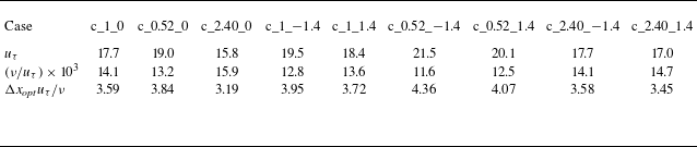Figure 8(b) illustrates the outcomes from sections taken along varying streamwise positions. It is evident that no consistent optimal phase shift value is observed across all cases, and the correlation coefficient does not experience a marked increase after the optimal phase shift, indicating that the relative forward movement of the pressure distribution with respect to height is confined to the streamwise direction. This aligns with the physical interpretation of the pressure stagnation point. Table 4 provides the viscous length dimensions and the optimal phase shift distances for each rough surface. Analogous to table 2, for the same $E{{S}_{z}}/E{{S}_{x}}$ , the viscous length dimension for the negative skewness is consistently the smallest (corresponding to the highest $u_{\tau }$ ). It is observed that all cases exhibit approximately the same dimensionless optimal phase shift distance (with each case having an identical grid scale within the rough surface), a phenomenon attributable to the uniform streamwise effective slope of all rough surfaces and the consistent inlet velocity profile. The pressure stagnation points, generated by the fluid’s impact upon the windward aspects of each rough peak, are statistically positioned at analogous locations. This indicates that the relative forward displacement of the pressure peak in relation to the height peak is unaffected by the spanwise effective slope and the skewness.

Table 3.

The correlation coefficients between the sheltering areas (subscript $s$ ) and the resistance peaks (subscript $f$ ) predicted by the new and old formulas on the rough surface.

3.2. Instantaneous physics of transition

In the context of flow transition with pressure gradient, the LSB emerges as a predominant feature, as depicted in figure 9(a). Figure 9(b) reveals that the LSB is generally confined to the interval $x\in [ 3,8 ]$ in the absence of a rough surface, where the spanwise uniformity of the streamwise velocity at the LSB’s trailing edge starts to deteriorate, akin to the observations of Hosseinverdi & Fasel (Reference Hosseinverdi and Fasel2019). In the absence of free-stream turbulence, the separated shear layer downstream is prone to K-H instability, leading to the breakdown of spanwise rollers and subsequent transition to turbulence. The y-value used for colouring indicates that the ratio of the LSB’s maximum height to the spanwise extent of the computational domain is approximately 16. According to previous studies (Jones, Sandberg & Sandham Reference Jones, Sandberg and Sandham2008; Hosseinverdi, Balzer & Fasel Reference Hosseinverdi, Balzer and Fasel2012), the spanwise range of the computational domain in this paper is sufficiently large to avoid influencing the LSB and its associated modal characteristics. Figure 9(b,c) also illustrates the distribution of the bottom wall’s streamwise friction coefficients under the nine rough surfaces. It is evident that there is no obvious LSB under these cases, implying that the rough surfaces, positioned near the peak velocity, disrupt the formation of the LSB and alter the transition from a separation-induced transition to a bypass one. Furthermore, it is observed that, with the exception of three cases of positive skewness, the other cases all yield countercurrent bottom-wall friction initiating at $x=2$ . Notably, the cases with the highest values were c_0.52_−1.4, c_1_−1.4 and c_0.52_0. The two cases of positive skewness, c_0.52_1.4 and c_2.40_1.4, also initiated reverse-flow friction from $x=3$ , yet only c_1_1.4 preserved forward-flow friction consistently. These observations suggest that the spanwise or streamwise wave features induced by $E{{S}_{z}}/E{{S}_{x}}$ can also generate local recirculation zones akin to those observed downstream of the large-scale depressions. Beyond $x\gt 5$ , all nine rough-surface cases exhibit steep increases of forward-flow friction, signalling the onset of transition. After $x\gt 8$ , the streamwise friction coefficient for all cases gradually stabilises, marking the conclusion of the transition and the onset of the turbulent phase.

Figure 8.

The p.d.f. of optimal phase shift $(N_p)$ values is presented for varying (a) spanwise and (b) streamwise positions across the rough surface (depicted by bar charts on the left ordinate and bottom abscissa). The absolute value of the correlation coefficient between rough-surface height and pressure coefficient distribution are illustrated (represented by curves and their corresponding filled areas on the right ordinate and top abscissa), with the black and blue regions signifying the results prior to and subsequent to the optimal phase shift, respectively.

In most cases, the hairpin vortex serves as a distinctive landmark of the transition’s onset. Figure 10 depicts the three-dimensional transient vortex structures, revealing distinct hairpin vortex formations across all cases. Notably, three negative skewness cases exhibit the densest hairpin vortex clusters, whereas those in cases of positive skewness are comparatively less dense. The central spanwise vorticity on the sidewall encapsulates the entire progression from the emergence of the spanwise rollers and hairpin vortices to their eventual dissolution. The vorticity distribution further suggests that there are no appreciable flow disruptions at the forefront and backend of the rough surface, signifying the successful mitigation by the implemented buffer slopes. Given that the spanwise vortex is a crucial component of the hairpin vortex’s head (Acarlar & Smith Reference Acarlar and Smith1987), three cases of negative skewness with great melt-down height yield the densest hairpin vortex clusters. This is evident in the distribution of spanwise vorticities, which are markedly uplifted in the downstream region of the rough surface prior to fragmentation. The increased elevation contributes to a greater velocity gradient within the free shear layer, thereby effectively intensifying the spanwise rollers and hairpin vortices. A comparison between the $E{{S}_{z}}/E{{S}_{x}}=0.52$ group and the $E{{S}_{z}}/E{{S}_{x}}=2.40$ group in figure 10 indicates that a larger $E{{S}_{z}}/E{{S}_{x}}$ value impedes the rise of spanwise rollers and the subsequent flow separation downstream of the rough surface, aligning with the findings of Jelly et al. (Reference Jelly, Ramani, Nugroho, Hutchins and Busse2022). It is noteworthy that in figure 10, c_2.40_0 and c_0.52_1.4 each generate a solitary hairpin vortex in the proximity of $z=1.5$ and $z=0.25$ , respectively. This occurrence is analogous to the single sequence of hairpin vortices produced by an isolated roughness element, both stemming from a robust streamwise vortex pair that forms downstream of a prominent rough peak as the flow passes around it. By examining the height distribution at the backend of these two rough surfaces, it becomes apparent that there are indeed local rough peaks at these spanwise locations (though the results are not depicted).

Table 4.

The friction velocities, viscous length scales and the optimal phase shift distances $(\Delta {{x}_{\textit{opt}}})$ normalised by the viscous length scales are presented for each rough surface.

Figure 9.

(a) The $u=0$ isosurface, devoid of roughness, is coloured with the y-coordinate. (b,c) The distribution of the bottom-wall streamwise coefficient at $z=1.5$ , under both the absence of rough surfaces and the presence of the nine rough-surface cases.

Figure 10.

The three-dimensional transient vortex structures for the nine rough-surface cases, ${{\lambda }_{2}}=-0.08$ , are visualised with colouring based on streamwise velocity. On the sidewall, the transient spanwise vorticity at $z=1.5$ is depicted, with the isosurface values ranging from $-8$ to 1. For ease of presentation, this is translated to the position $z=0$ .

Cohen et al. (Reference Cohen, Karp and Mehta2014) identified the three components of the hairpin vortex as counter-rotating vortex pairs, wall-normal shear and two-dimensional spanwise vortex sheets. We proceeds to investigate them individually using the methodology of Bucci et al. (Reference Bucci, Cherubini, Loiseau and Robinet2021). In light of the flow characteristics related to transition observed in figure 9(b,c), these primarily manifest in the $x\in [ 2,10 ]$ region. For the range of wall-normal heights, the wall-normal truncation employed by Shahinfar et al. (Reference Shahinfar, Fransson, Sattarzadeh and Talamelli2013) in their study of streaks is adopted here $\colon$

(3.7) \begin{equation} {0\leqslant \eta \leqslant {{\eta }^{*}}}, \end{equation}

where

(3.8) \begin{equation} {\eta =\frac {y}{\delta }=\frac {y}{\sqrt {x\nu /{{U}_{\infty }}}},{{\eta }^{*}}=9}. \end{equation}

in which $\delta$ denotes the square root of distance from the leading edge of the boundary layer. It can be inferred that the wall-normal truncation range corresponding to the $x\in [ 2,10 ]$ region is $y\in [ 0.20,0.45 ]$ . Figure 11 captures the average $y=0.3$ of this truncation range, which is employed to illustrate the streamwise vorticity distribution, thereby ensuring that the flow characteristics are maximally demonstrated. As evident from figure 11, the streamwise vortex pairs generated by c_0.52_−1.4, c_2.40_−1.4 and c_0.52_0 exhibit the highest overall strength, whereas those generated by c_2.40_0, c_1_1.4 and c_0.52_1.4 demonstrate the weakest. The findings indicate that a small $E{{S}_{z}}/E{{S}_{x}}$ value and negative skewness exert an excitatory effect on streamwise vortices, whereas the spanwise modulation of a rough surface with a large $E{{S}_{z}}/E{{S}_{x}}$ value can significantly impede the growth of such vortices, consequently hindering the formation of hairpin vortices.

Figure 11.

The transient streamwise vorticity isosurface for each case is denoted at $y=0.3$ . Additionally, a top-down view of the rough surface has been incorporated to enhance visual clarity.

Figure 12.

The distribution of transient streamwise velocity (blue solid line) and spanwise vorticity (green dash-dot line) at various longitudinal positions is presented. Each pair of curves horizontally represents the corresponding distribution values, with the data being averaged across the spanwise direction. The inflection points in the streamwise velocity distribution are denoted by open circles, whereas the extremities of the spanwise vorticity are indicated by open triangles. These points are identified based on the zero-crossings of the second derivative for inflection points and the first derivative for extremities.

The subsequent analysis explores the characteristics of wall-normal shear and two-dimensional spanwise vortex sheets. Figure 12 depicts the distribution of streamwise velocity and spanwise vorticity along five longitudinal locations. Under the negative skewness cases, the streamwise velocity at $x=2$ is significantly higher than that observed in other cases. This aligns with the augmented spanwise vorticity distribution presented in figure 10, which can be attributed to the increased melt-down height associated with negative skewness. At $x=3$ , c_1_−1.4, c_2.40_−1.4 and c_2.40_1.4 commence the manifestation of multiple velocity inflection points and vorticity extremities, whereas the velocity distributions for the remaining cases preserve a solitary inflection point. This suggests that negative skewness and large $E{{S}_{z}}/E{{S}_{x}}$ values can foster the formation of two-dimensional spanwise vortex sheets. Beyond $x\gt 3$ , there is a significant rise in the number of velocity inflection points across all cases, and the spanwise vorticity distribution becomes increasingly distorted, coinciding with the widespread appearance of hairpin vortices as depicted in figure 10. At the $x=4,5$ positions within the hairpin vortex cluster, c_1_−1.4 and c_2.40_−1.4 exhibit the most pronounced distortion in spanwise vorticity distribution and the highest inflection point, while c_0.52_0 presents the lowest velocity inflection point and the least degree of distortion in the spanwise vorticity distribution. Hence, it is deduced that the streamwise modulation of a small $E{{S}_{z}}/E{{S}_{x}}$ value can curtail the deformation of wall-normal shear and the two-dimensional spanwise vortex sheet, whereas larger $E{{S}_{z}}/E{{S}_{x}}$ values and negative skewness exert opposite effects. In essence, the influence of $E{{S}_{z}}/E{{S}_{x}}$ on the streamwise vortex pair counters the effects on the wall-normal shear and the two-dimensional spanwise vortex sheet. Negative skewness uniquely stimulates all three components of the hairpin vortices, thereby accounting for the densest clusters of hairpin vortices observed in the three negative skewness cases depicted in figure 10.

3.3. First and second moments

To delve further into the impact of varying ${E{{S}_{z}}}/{E{{S}_{x}}}$ and $Sk$ on the flow characteristics within the peak velocity region and its downstream vicinity, an analysis of the first and second moments of the flow is conducted. Initially, the secondary flow dynamics over the rough surface are investigated, with the imaginary part of the complex conjugate eigenvalues of the two-dimensional time-averaged velocity gradient tensor (Jelly et al. Reference Jelly, Ramani, Nugroho, Hutchins and Busse2022). The pertinent formulas are as follows $\colon$

(3.9) \begin{align}{ \qquad\qquad\qquad\qquad\,\,\,\,{\overline {{{{\varLambda } }_{ci}}} ={{\lambda }_{ci}}{{{\varOmega } }_{x}}/\left | {{{\varOmega } }_{x}} \right |},\\[-12pt]\nonumber } \end{align}

(3.10) \begin{align}{\qquad\qquad\qquad\qquad{\boldsymbol{\nabla }{\boldsymbol{u}_{2{\textrm{D}}}} =\left [ \begin{matrix} \dfrac {\partial V}{\partial y} & \dfrac {\partial V}{\partial z} \\[12pt] \dfrac {\partial W}{\partial y} & \dfrac {\partial W}{\partial z} \\ \end{matrix} \right ] },\\[-12pt]\nonumber} \end{align}

(3.11) \begin{align}{{{{\lambda }^{2}}+p\lambda +q=0,\text{ }{{\lambda }_{1,2}} =\frac {-p\pm i\sqrt {4q-{{p}^{2}}}}{2},\text{ }{{\lambda }_{ci}}=\frac {\sqrt {4q-{{p}^{2}}}}{2}}, } \end{align}

where

(3.12) \begin{equation} {p=-\left ( \frac {\partial V}{\partial y}+\frac {\partial W}{\partial z} \right ),\text{ }q=\frac {\partial V}{\partial y}\frac {\partial W}{\partial z}-\frac {\partial V}{\partial z}\frac {\partial W}{\partial y}}, \end{equation}

where $V$ is time-averaged wall-normal velocity, $W$ is time-averaged spanwise velocity, $\lambda$ is the variable of eigenvalue equation, $\overline {{{\varLambda }_{ci}}}$ represents the signed swirling strength, ${\lambda }_{ci}$ denotes the imaginary part of the eigenvalue, and ${\varOmega }_{x}$ signifies the time-averaged streamwise vorticity. Equation (3.11) represents the eigenvalue equation associated with the two-dimensional time-averaged velocity gradient tensor and its complex conjugate eigenvalue solution. The coefficient ${{{\varOmega } }_{x}}/\left | {{{\varOmega } }_{x}} \right |$ is introduced to ensure that the depicted secondary flow aligns with the local time-averaged streamwise vorticity. The findings are presented in figure 13. When comparing the cases with identical skewness, it becomes evident that a decrease in ${E{{S}_{z}}}/{E{{S}_{x}}}$ leads progressively to a progressive rarefaction of the secondary flow pattern. This is because the streamwise wavelength structure becomes more pronounced as ${E{{S}_{z}}}/{E{{S}_{x}}}$ diminishes, thereby restraining the evolution of the secondary flow pattern along the streamwise direction, in agreement with the observations of Jelly et al. (Reference Jelly, Ramani, Nugroho, Hutchins and Busse2022). When contrasting cases with the same $E{{S}_{z}}/E{{S}_{x}}$ , positive skewness is observed to enhance the continuity of the secondary flow pattern. This can be explained by the local recirculation within the pits, which hinders the cohesive development of the quasi-streamwise vortices downstream. The results for c_0.52_1.4 further illustrate that, despite the impediment posed by the streamwise wave topography with low $E{{S}_{z}}/E{{S}_{x}}$ modulation, positive skewness can still yield a secondary flow pattern with considerable continuity, suggesting that the governing factor in this regard is the skewness.

Figure 13.

The secondary flow in the vicinity above each rough surface is visualised through the isosurface of the signed swirl intensity, $\overline {{{{\varLambda } }_{ci}}}=\pm 0.2$ , with yellow indicative of negative values and blue signifying positive values.

For three-dimensional rough surfaces, a pivotal first moment of interest is the dispersive quantity, which is derived from the spatial averaging of the time-averaged quantity, as follows (Jelly et al. Reference Jelly, Ramani, Nugroho, Hutchins and Busse2022) $\colon$

(3.13) \begin{align}{ {\left \langle {{U}_{i}} \right \rangle \left ( y \right ) =\frac {1}{{{A}_{f}}\left ( y \right )}\int _{{{A}_{f}}\left ( y \right )}{{{U}_{i}}\left ( y \right ){\textrm d}x{\textrm d}z}}, } \end{align}

(3.14) \begin{align}{{\widetilde {{{U}_{i}}} ={{U}_{i}}-\left \langle {{U}_{i}} \right \rangle }, } \end{align}

where $U_i$ denotes the time-averaged streamwise velocity, $\left \langle \boldsymbol{\cdot }\right \rangle$ denotes the fluid-only integral average at a specific height, ${{A}_{f}} ( y )$ signifies the area occupied by the fluid at that height, and $\widetilde {{{U}_{i}}}$ represents the dispersive velocity. In this study, ${{A}_{f}} ( y )$ specifically refers to the fluid area within the range of rough-surface projection. Figure 14 illustrates the distribution of streamwise dispersive velocity across the central cross-section of the rough surface. From the observation of the cases with the same skewness, it is evident that, in alignment with the influence of the aforementioned secondary flow patterns, a decrease in ${E{{S}_{z}}}/{E{{S}_{x}}}$ leads to a sparser streamwise dispersive velocity. Nevertheless, the upper height limit of the streamwise dispersive velocity distribution remains essentially constant, approximately at $0.2H$ , and is unaffected by variations in ${E{{S}_{z}}}/{E{{S}_{x}}}$ and skewness, a departure from the findings of previous studies (Chan et al. Reference Chan, Macdonald, Chung, Hutchins and Ooi2018; Jelly et al. Reference Jelly, Ramani, Nugroho, Hutchins and Busse2022). It is crucial to note that the rough surface near the peak velocity has not experienced transition; transition begins only downstream of the rough surface, as evidenced by the results in §3.2. However, prior research monitored the dispersive velocity in full turbulence, where the degree of momentum diffusion to the outer layer of the boundary layer differs. When comparing cases with positive and negative skewness, it is apparent that positive skewness enhances the prevalence of positive streamwise dispersive velocities, countering the negative dispersive velocities (arising from local recirculation) induced by negative skewness. Skewness predominantly governs the homogeneity of the streamwise dispersive velocities.

Figure 14.

The contour of streamwise dispersive velocity $\widetilde {U}$ on the central cross-section in the range of the rough surface, $x=1$ .

Since (3.14) defines the dispersive velocity, the dispersive stress can be further defined as

(3.15) \begin{equation} {{\boldsymbol{D}_{ij}}=\left \langle \left ( {{U}_{i}}-\left \langle {{U}_{i}} \right \rangle \right )\left ( {{U}_{\!j}}-\left \langle {{U}_{\!j}} \right \rangle \right ) \right \rangle =\left \langle \widetilde {{{U}_{i}}}\widetilde {{{U}_{\!j}}} \right \rangle }. \end{equation}

Figure 15 presents three types of dispersive normal stresses. It is evident that the magnitude of the streamwise dispersive normal stress exceeds that of the spanwise and wall-normal stresses, due primarily to the streamwise pressure gradient. In ${D}_{11}$ , c_1_1.4 demonstrated the highest degree of spatial heterogeneity, with c_2.40_1.4 and c_0.52_1.4 following suit. The streamwise velocity spatial uniformity in the remaining cases was approximately equivalent. This suggests that positive skewness is the predominant influence on the streamwise dispersive normal stress. For the distribution of ${D}_{22}$ , the peak values are observed in the three cases with negative skewness, signifying that extensive depressions markedly enhance the spatial heterogeneity of the wall-normal velocity. The c_1_0 exhibits the lowest values for both the streamwise and wall-normal dispersive normal stress peaks. For ${D}_{33}$ , the maximum peaks are found in the three cases characterised by positive skewness, whereas the three cases with negative skewness exhibit the lowest peaks. This suggests that, in relation to the spanwise spatial heterogeneity perpendicular to the driving pressure gradient, the numerous elevated regions induced by negative skewness can markedly diminish the spanwise spatial non-uniformity.

Figure 15.

The dispersive stress across each rough surface is distributed along the wall-normal direction, with the stress being non-dimensionalised by $u_{\tau }^{2}$ and the y-coordinate by $\nu /{{u}_{\tau }}$ .

Subsequently, we direct our focus to the transition region located downstream of the rough surface. The most frequently employed second moments for studying transition are the Reynolds stress and the fluctuating kinetic energy (FKE) equations $\colon$

(3.16) \begin{equation} {\frac {\partial k}{\partial t}+{{U}_{\!j}}\frac {\partial k}{\partial {{x}_{\!j}}}=\underbrace {-\overline {{{u}_{i}^{\prime }}{{u}_{\!j}^{\prime }}}\frac {\partial {{U}_{i}}}{\partial {{x}_{\!j}}}}_{{{P}_{k}}}-\frac {1}{2}\frac {\partial \overline {{{u}_{i}^{\prime }}{{u}_{i}^{\prime }}{{u}_{\!j}^{\prime }}}}{\partial {{x}_{\!j}}}-\frac {1}{\rho }\frac {\partial \overline {{p}^{\prime }{{u}_{\!j}^{\prime }}}}{\partial {{x}_{\!j}}}+\nu \frac {{{\partial }^{2}}k}{\partial {{x}_{\!j}}\partial {{x}_{\!j}}}\underbrace {-\nu \overline {\frac {\partial {{u}_{i}^{\prime }}}{\partial {{x}_{\!j}}}\frac {\partial {{u}_{i}^{\prime }}}{\partial {{x}_{\!j}}}}}_{{{\varepsilon }_{k}}}}, \end{equation}

where $p^{\prime}$ is the fluctuating pressure, ${u}_{i}^{\prime }$ denotes the fluctuating velocity, $k=\overline {{{u}_{i}^{\prime }}{{u}_{i}^{\prime }}}/2$ represents the FKE, while ${P}_{k}$ and ${\varepsilon }_{k}$ correspond to the production and dissipation terms, respectively. The former encapsulates the interaction between the time-averaged strain rate and the Reynolds stress, whereas the latter signifies the dissipation of FKE due to viscous action. As observed in §3.2, flow characteristics pertinent to transition emerge predominantly within the $x\in [ 2,10 ]$ region. To ascertain the local spatial position that encapsulates the characteristics most effectively, the power spectrum (PS) of the flow intensity, obtained via Fourier transform, is employed as depicted in figure 16. The flow intensity is defined as follows $\colon$

(3.17) \begin{equation} {Fi=\sqrt {\frac {1}{3}\frac {{{u}^{2}}+{{v}^{2}}+{{w}^{2}}}{U_{\infty }^{2}}}}. \end{equation}

where $w$ denotes the spanwise velocity. Evidently, the predominant frequencies across all cases fall within the spectrum of $\omega \in [ 1,10 ]$ . As illustrated later in figures 22 and 23, these frequencies are predominantly clustered within the range of $\omega =2{\sim}7$ . This finding contrasts markedly with the results reported by Bucci et al. (Reference Bucci, Cherubini, Loiseau and Robinet2021), where the dominant frequencies for the isolated cylinder they examined were grouped primarily within the range of $\omega =0.4{\sim}2$ ( ${\textit{Re}}=700,1000$ ). The characteristic frequencies of the rough surfaces in this study, under linear dynamic approximation, are nearly an order of magnitude greater than those of the isolated cylinder. The predominant frequency and amplitude are observed at the two positions $x=4,6$ across almost all cases, and subsequent investigation into transition characteristics concentrates on these two streamwise locations. It is further noticed that at $x=2$ , only the PS of c_2.40_0 exhibits notable amplitudes, which correspond to the solitary hairpin vortex that emerges at $z=1.5$ , as depicted in figure 10. In the downstream region of $x=8,10$ , the dominant amplitude of the PS diminishes substantially, with several dominant frequencies no longer present. This can be attributed to the fact that turbulence resulting from bypass transition lacks characteristic frequencies in the absence of free-stream turbulence at the inlet and without specific elements such as jets or vibrating walls within the computational domain.

Figure 16.

The three-dimensional PS distribution of the flow intensity for five spatial points within the domain has been computed, with data extracted from the statistical equilibrium. Here, $x\in [ 2,10 ]$ , $z=1.5$ . The y-coordinates correspond to half the wall-normal height as truncated by (3.7) and (3.8), while $\omega$ denotes the circular frequency.

Figure 17.

The isosurface of the FKE production term and the isoline of the dissipation term at (a) $x=4$ and (b) $x=6$ of each case.

The distribution of the FKE production and dissipation terms at the two positions $x=4,6$ is depicted in figure 17. As indicated by the figure’s legends, the absolute values of these terms at $x=4$ are substantially greater than those at $x=6$ , owing to the fact that the early transition stage predominantly involves the transformation of time-averaged kinetic energy into FKE. When the time-averaged energy conversion occurs via the production term opposite in sign to ${P}_{k}$ in the time-averaged kinetic energy budget equation, the subsequent dissipation of FKE through viscous action also intensifies. In figure 17(a), c_0.52_−1.4 stands out exhibiting significantly higher production and dissipation terms than the other cases. Drawing upon the transient physical analysis in §3.2, it is indicative that the conjunction of smaller $E{{S}_{z}}/E{{S}_{x}}$ values and negative skewness can optimise the production of FKE within the immediate downstream. The observed phenomenon is clearly associated with K-H instability. Non-negligible dissipation terms are present near the bottom wall of cases of negative skewness, signifying that the viscous instability prompted by the lift-up mechanism contributes significantly. Comparing the cases with identical skewness, it is evident that the spanwise modulation of higher $E{{S}_{z}}/E{{S}_{x}}$ values leads to a reduction in the spanwise wavelength of both the production and dissipation terms, echoing the influence on the secondary flow pattern in figure 13. At $x=6$ , the dissipation terms of all cases trend towards the bottom wall, a phenomenon explainable by the definitions in (3.16) $\colon$ the fluctuating velocity distributed in the domain during the later stages of transition increases markedly, and the fluctuating velocity gradient near the bottom wall becomes predominant. Compared with $x=4$ , the production term for each case is more diffused, with a reduced spanwise wavelength, a consequence of the decreased energy input from the time-averaged kinetic energy and the enhanced diffusion term due to the increasing fluctuating velocity itself. Figure 18 depicts the distributions of Reynolds stresses $\overline {{u}^{\prime }{u}^{\prime }}$ and $\overline {{v}^{\prime }{w}^{\prime }}$ for the two longitudinal directions, which, when contrasted with figure 17 , exhibit a similar pattern to the production terms, particularly at $x=6$ . This suggests that the previous explanation regarding the concentration of dissipation terms at the bottom wall is accurate.

Figure 18.

Reynolds normal stress $\overline {{u}^{\prime }{u}^{\prime }}$ contour and Reynolds shear stress $\overline {{v}^{\prime }{w}^{\prime }}$ isoline at (a) $x=4$ and (b) $x=6$ of each case.

3.4. Coherent structures of transition

Coherent structures are distinctive features of transitional flows, characterised by the cyclic amalgamation of streamwise vorticity and streaks derived from the lift-up mechanism (Bae, Lozano-Durán & Mckeon Reference Bae, Lozano-Durán and Mckeon2021). Investigating the spatial wavelengths and temporal frequencies of these coherent structures can deepen our understanding of varied impacts of ${E{{S}_{z}}}/{E{{S}_{x}}}$ and $Sk$ on transition onset. Returning to the two cross-sections, the premultiplied power spectra of the three types of fluctuations for each case are presented in figure 19. As with the findings in figures 17 and 18, c_0.52_−1.4 continues to exhibit the highest values at $x=4$ . A comparison of the wavenumbers in the peak region for the two longitudinal locations reveals that the characteristic wavenumber at $x=4$ is approximately 20–40, diminishing to 10–20 at $x=6$ . Furthermore, the intensity of PS across various cases exhibits a trend towards uniformity. This aligns with the changes observed in the production term distribution of figure 17, resulting primarily from the reduction in time-averaged input energy and the increased influence of the diffusion term. It is also evident that the frequency band of the peak region for three cases of negative skewness at $x=4$ is significantly broader than that of the other cases, suggesting that large-scale pits facilitate the growth of the spanwise wave of coherent structures.

Figure 19.

The premultiplied power spectra of three types of fluctuations are depicted at (a) $x=4$ and (b) $x=6$ for each case, with the streamwise fluctuation power spectra $(\phi_{u^{\prime}u^{\prime}})$ represented by isosurfaces, and the wall-normal fluctuation power spectra $(\phi_{v^{\prime}v^{\prime}})$ and spanwise fluctuation power spectra $(\phi_{w^{\prime}w^{\prime}})$ by red and green isolines, respectively. $k_{z}$ represents the spanwise wavenumber. Bidirectional arrows denote the bandwidth of each peak region.

Figure 20.

The autocorrelations of the three fluctuating velocities at positions (a) $x=4$ and (b) $x=6$ are exhibited. $R_{u^{\prime}u^{\prime}}$ , $R_{v^{\prime}v^{\prime}}$ , and $R_{w^{\prime}w^{\prime}}$ denote the autocorrelations of the streamwise, wall-normal, and spanwise fluctuating velocities, respectively. $t$ represents the time. Data are extracted from the statistical equilibrium, with the y-coordinates representing half the truncated wall-normal height as shown in (3.7) and (3.8), and with the x-coordinates in the range of $x\in [ 2,10 ]$ and the z-coordinates of $z=1.5$ . The Fourier transform is utilised to derive the spectral distribution of each curve, and the circular frequencies associated with the peak spectral magnitudes are represented by the top abscissa of this figure. Here, $\omega$ corresponds to the circular frequency.

Let’s focus on the time integral scale of coherent structures. Figure 20 presents the autocorrelation curves of the fluctuating velocity over time for the two cross-sections. Regarding the integral scale from the first instance of decay to zero, the three cases with negative skewness each exhibited the smallest integral scale for the three fluctuating velocities at $x=4$ , in alignment with the densest vortex clustering observed in figure 10 for the negative skewness cases. It is also obvious that the three cases with positive skewness generally presented larger integral scales for the three fluctuating velocities. Utilising a threshold value of 0.2 to calculate the integral scale (Yang et al. Reference Yang, Stroh, Chung and Forooghi2022), as depicted in figure 21, essentially confirms the aforementioned findings, save for the c_1_1.4, which displays a smaller integral scale for the three fluctuating velocities at $x=4$ . This suggests a significant reduction in the temporal integral scale of coherent structures for the negative skewness cases, while in the positive skewness ones, the temporal integral scale of coherent structures within the transitional region is prolonged to the greatest extent. For the $x=6$ cross-section, the previous conclusions no longer hold, and the influence of the statistical properties of the rough surface on the integration scale is no longer predominant. The frequencies corresponding to the maximum spectrum values of each curve are also provided in figure 20, serving as an approximation of the frequency characteristics of the three fluctuating velocities at the respective spatial points. It is evident that the three fluctuation frequencies for cases of negative skewness at $x=4$ are basically the highest. This echoes the extensive distribution of production and dissipation terms in the negative skewness cases depicted in figures 17 and 18, which is intricately linked to inviscid instability (Hosseinverdi & Fasel Reference Hosseinverdi and Fasel2019).

Figure 21.

The time integral scale ( $L_R$ ) of each curve in figure 20 is calculated with the threshold of 0.2 reduced for the first time: (a) $x=4$ , (b) $x=6$ .

Figure 22.

The distribution of wall-normal heights corresponding to the peak PS of the streamwise fluctuating velocity across a total of 50 cross-sections within the range of $x\in [ 2,10 ]$ is examined. The hollow triangular curve plotted against the right ordinate denotes the respective PS values, while the colour of the filled circles signifies the spanwise wavenumber associated with each maximum value.

The evolution of spanwise wavelength and the predominant wall-normal height along the streamwise direction of coherent structures is depicted in figure 22. Notably, c_2.40_0 exhibits a high spanwise wavenumber of approximately 14 within the interval $x\in [ 4,6 ]$ , where the PS attains its peak value. The corresponding wavelength constitutes roughly 15% of the spanwise extent of the computational domain. The spanwise wavenumbers for c_0.52_-1.4 and c_0.52_1.4 are comparatively lower, while the remaining cases feature spanwise wavenumbers tending towards zero in the vicinity of the peak PS, suggesting that the coherent structures do not possess a defined spanwise wavelength. This finding indicates that significant spanwise modulation by large $E{{S}_{z}}/E{{S}_{x}}$ values can directly yield coherent structures with high spanwise wavenumbers, whereas extensive depressions or rough peaks can impede this process. The wall-normal height curve reveals that the high spanwise wavenumbers of c_2.40_0 are concentrated in the range of $y\in [ 0.1,0.2 ]$ , signifying that the corresponding coherent structures are consistently positioned at the core of the FKE production, dissipation and Reynolds stress peak regions, as illustrated in figures 17 and 18.

3.5. Characteristic modal analysis

The preceding analysis of transition has centred primarily on local flow structures or individual fluctuating velocity fields, whereas the characteristic modes derived from the complete three-dimensional velocity field can offer novel perspectives on the influence of ${E{{S}_{z}}}/{E{{S}_{x}}}$ and $Sk$ on transition phenomena. This paper employs DMD to investigate these eigenmodes. The algorithmic approach, detailed in the work of Schmid (Reference Schmid2010), constitutes a widely adopted numerical framework for Koopman analysis and is capable of approximating the dynamics of nonlinear systems with linear dynamics (Loiseau Reference Loiseau2014). The standard parameters utilised in DMD analysis include modal amplitude and modal growth rate, which indicate the mode’s contribution to a chosen snapshot and its linear stability, respectively. Without loss of generality, the first snapshot is selected to define the modal amplitude (Taira et al. Reference Taira, Hemati, Brunton, Sun, Duraisamy, Bagheri, Dawson and Yeh2020), with the specific formulas as follows:

(3.18) \begin{align}{ {b_{i}^{0} =\boldsymbol{\psi } _{i}^{-1}{\boldsymbol{X}_{0}}}, } \end{align}

(3.19) \begin{align}{ {{{\lambda }_{i}} ={{e}^{{{\mu }_{i}}\Delta t}}, \text{ }{{g}_{i}}={\textit{Re}}\left ( {{\mu }_{i}} \right )=\frac {\ln \left | {{\lambda }_{i}} \right |}{\Delta t}}, } \end{align}

where ${b}_{i}$ denotes the amplitude of the ith mode, while $\boldsymbol{\psi }_{i}$ corresponds to the ith mode. The superscript $-1$ signifies the inverse matrix; $\boldsymbol{X}_{0}$ refers to the initial snapshot of the input data, and ${\lambda }_{i}$ represents the Ritz eigenvalue associated with the ith mode (Hosseinverdi & Fasel Reference Hosseinverdi and Fasel2019), which is the eigenvalue of the linear coefficient matrix within a linear system; ${\mu }_{i}$ constitutes the exponential component of ${\lambda }_{i}$ , ${g}_{i}$ is the modal growth rate, and $\textit{Re} ( \boldsymbol{\cdot })$ indicates the complex real part; $\Delta t$ is the temporal increment between snapshots. In this paper, the temporal increment $\Delta t=3\times {{10}^{-2}}$ corresponds to capturing a snapshot every 100 computational steps. In relation to the minimum time integral scale ${{L}_{R,min }}\approx 0.08$ depicted in figure 21, then ${{L}_{R,min }}\approx 2.7\Delta t$ . Figure 23 illustrates the convergence of DMD results with respect to $\Delta t$ , with the total duration of the time series set at three. Eigenvalue spectra were computed for five distinct snapshot sampling intervals. It is evident that all eigenvalues tend towards a common fitted curve, signifying that the chosen ${{N}_{\Delta t}}=100$ for this study ensures sufficient convergence of the DMD outcomes. It is important to note that due to varying sampling intervals, the number of snapshots employed to derive the approximate linear dynamics from the same time series differs, resulting in the eigenvalue spectra’s inability to fully coincide. Nonetheless, they are expected to converge towards a consistent solution.

Figure 23.

At (a) $x=4$ and (b) $x=6$ , the DMD eigenvalue spectra for the c_1_0 are presented across varying snapshot time steps (only the third quadrant of the complex plane depicted). $\mu_{i,i}$ is the imaginary part of the eigenvalue exponential component, and ${\mu}_{i.r}$ is the corresponding real part. The time series length is fixed at 3. Here, ${N}_{\Delta t}$ denotes the ratio of the snapshot time step to the computational time step. The solid line signifies the spline-fitted curve.

Figures 24 and 25 present the DMD results for two cross-sections at $x=4,6$ , compared with the PS values from figure 16. Initially, the modal growth rates are examined. The unstable modes of c_2.40_−1.4 and c_2.40_0 are particularly pronounced, occurring predominantly within the range of $\omega \in [2,7]$ . In contrast, c_1_0 and c_0.52_1.4 do not exhibit substantial modal growth rates exceeding zero. This suggests that the coherent structure’s spanwise wave fostered by large $E{{S}_{z}}/E{{S}_{x}}$ exhibits a pronouncedly unstable tendency. Nevertheless, the streamwise modulation induced by small $E{{S}_{z}}/E{{S}_{x}}$ and the rough peaks can effectively curtail this instability. Moreover, the large modal amplitudes and large growth rates across various cases fall predominantly within the same frequency domain. The colour bars in the figure indicate the PS values, which reflect the intensity of the nonlinear coherent structure. In figures 24 and 25, the frequencies with substantial modal amplitude and high PS values are highlighted, $\omega =2,4.5\,{\textrm{and}}\,7$ . At these three characteristic frequencies, the linear modes may exhibit a quasi-orthogonality with respect to other DMD modes and can independently approximate the nonlinear dynamic evolution (Bucci Reference Bucci2017).

Figure 24.

The distribution of DMD modal amplitude and growth rate of flow intensity along the frequency axis is depicted, with solid squares denoting the modal amplitude and hollow circles the modal growth rate. The left ordinate represents the modal amplitude $(b^0)$ , and the right ordinate represents the modal growth rate $(g)$ . The colour bar illustrates the PS values of the flow intensity at each frequency, while the vertical dashed line indicates the three frequencies of particular interest. Here, $x=4$ , and $\omega$ corresponds to the circular frequency.

Figure 25.

The distribution of DMD modal amplitude and growth rate of flow intensity along the frequency axis at $x=6$ is depicted, with the legends equal to that in figure 24.

To delve further into the aforementioned issues, the real components of the corresponding Fourier series coefficients (termed shape functions) are extracted from the three distinctive frequencies indicated in figures 24 and 25, and are then compared with the real parts of the DMD modes at the same frequencies. The findings are presented in figures 26 and 27. According to the legends, it is observed that the characteristic modes corresponding to the three frequencies exhibit a sequential decrease in overall values. The distribution of DMD modes and shape functions across all cases exhibits a degree of similarity. Figure 28 reveals the specific correlation coefficients. Clearly, the correlation coefficients for some cases exceed 0.5, signifying that the corresponding DMD modes exhibit a degree of quasi-orthogonality.

Figure 26.

The real component of the DMD mode of flow intensity at $x=4$ across various frequencies is compared with the real part of the Fourier series coefficients $(\textit{Fi}_\textit{fft})$ . The isoline denotes the real component of the DMD mode, while the isosurface signifies the real part of the Fourier series coefficients. The sequence of cases from top to bottom at each frequency corresponds to the arrangement specified in table 1.

Figure 27.

The real component of the DMD mode of flow intensity at $x=6$ across various frequencies is compared with the real part of the Fourier series coefficients, with the legends equal to that in figure 26.

Figure 28.

At (a) $x=4$ and (b) $x=6$ , the correlation coefficients $(\sigma^*)$ between the real components of DMD modes and the real parts of Fourier series coefficients across distinct frequencies are presented. The sequence of cases from left to right at each frequency corresponds to the arrangement specified in table 1. Within the figure, the three negative skewness cases are denoted by $\dagger$ .

Initially, a comparison of the nine rough-surface cases at each characteristic frequency reveals that the DMD flow intensity for three cases of negative skewness under frequencies $\omega =4.5$ and $\omega =7$ at $x=4$ is substantially higher than that of the other cases. However, no such pronounced discrepancy is observed under $\omega =2$ . In conjunction with figure 24, this is intricately linked to the PS values of the flow intensity. This finding suggests that during the initial phase of transition, negative skewness is capable of generating linear modes of equivalent intensity to the nonlinear coherent structures at middle and high frequencies. At $x=6$ , the DMD flow intensities for the three characteristic frequencies under negative skewness cases are comparable to those under other cases. In light of the generally higher correlation coefficients at middle and high frequencies for the negative skewness cases depicted in figure 28(a), it can be inferred that negative skewness fosters the generation of linear modes with quasi-orthogonality. Furthermore, in the later stages of transition, zero skewness appears to generate linear modes with a strong degree of quasi-orthogonality at low frequencies.