Hydrodynamics and Navier–Stokes equations

The continuum hypothesis that fluid properties, such as density, velocity, temperature, and pressure, are well defined at infinitesimally small points and vary continuously from one point to another, is at the heart of classical hydrodynamics. ^{Reference Batchelor27} In most applications of fluid mechanics, the physical dimensions of the flow are extremely large compared to the molecular size and mean free path. Based on these assumptions, changes in flow properties are regarded as continuous, hence the continuum assumptions work well from the macroscale down to the microscale and even to the scale of a few nanometers. As a consequence, the Navier–Stokes differential equations based on the continuum hypothesis are used to solve hydrodynamic problems over a large range of length scales.

Hydrodynamic boundary condition

The hydrodynamic boundary condition (BC) is at the core of slip and flow enhancement of water in CNTs. It has been a subject of significant interest in recent times, even though the problem of formulating the BC has existed since the beginning of the 18th century. ^{Reference Kannam28} The fluid transport coefficients along with the BC are used in the Navier–Stokes equations to solve for flow properties. The transport coefficients are intrinsic to the nature of the fluid, and there are several methods of measuring them accurately.

The BC is generally not derived from first principles, hence one often assumes the no-slip BC, according to which the normal component of the fluid velocity vanishes and the tangential velocity of the fluid relative to the adjacent solid is zero irrespective of the nature of both the fluid and solid. The no-slip BC leads to an exact analytical solution for some simple hydrodynamic problems. The general BC often used was first expressed by Navier using a quantity called slip length, l _s , defined as:

(1) $${l_s} = {\eta \over \zeta }\,,$$

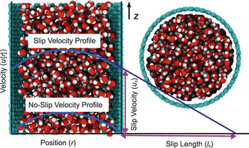
where ζ is the interfacial friction coefficient at the fluid–solid interface and η is the fluid shear viscosity. ^{Reference Navier29} The slip length is defined as the length extrapolated into the wall at which the fluid velocity would be zero, assuming a linear extrapolation, as depicted in Figure 1 .

Figure 1.

Schematic representation of water flow through carbon nanotubes (Poiseuille flow). The velocity profiles with and without slip, slip length (l _S ), slip velocity (u _S ), and velocity with respect to position (u _r ) are depicted in the figure.

Hagen–Poiseuille flow

Hagen–Poiseuille flow refers to fluid flow between two parallel walls or in a cylindrical tube, such as water in CNTs under a pressure gradient. Consider the case where a fluid is confined in a cylindrical tube of radius, r _t , and acted on by a uniform external field, F ^e (or a pressure gradient) along the z direction (see Figure 1). For this case, the Navier–Stokes equation reduces to the Stokes (or Poisson) equation, which in cylindrical coordinates (r, θ, z) is:

(2) $${1 \over r}{\partial \over {\partial r}}\left( {r{{\partial {u_z}\left( r \right)} \over {\partial r}}} \right) = - {{\rho {F^e}} \over \eta }\,,$$

where ρ is the fluid density and it is assumed that u _z (r) (which represents flow in the z direction) must be finite at r = 0. Applying the no-slip BC (i.e., the fluid velocity at the wall r = r _t is zero), yields the solution:

(3) $${u_z}\left( r \right) = \left( {{{\rho {F^e}} \over {4\eta }}} \right)\left( {r_t^2 - {r^2}} \right)\,.$$

The velocity profile across the tube is parabolic with maximum at the tube center r = 0 and zero at the tube surface r = r _t . The mass flow rate through the tube can be obtained by integrating the velocity profile over the tube’s cross-sectional area.

Slip and flow enhancement

When the fluid has a nonzero velocity at the wall surface (slip velocity, see Figure 1), the velocity profile becomes:

(4) $${u_z}\left( r \right) = \left( {{{\rho {F^e}} \over {4\eta }}} \right)\left( {r_t^2 - {r^2}} \right) + {u_s}\,,$$

where u _s is the slip velocity (i.e., the velocity of the fluid at the fluid–wall interface). Here, the fluid viscosity is assumed to remain the same in the presence of slip. The slip length and slip velocity are related via:

(5) $${u_s} = {u_z}\left( {{r_t}} \right) = {l_s}{\left( {{{\partial {u_z}} \over {\partial r}}\left( r \right)} \right)_{r\, = \,{r_t}}}\,.$$

The mass flow rate is enhanced in the presence of slip and the ratio of observed flow rate Q _slip (in the presence of slip) to the expected flow rate Q _no-slip (with no-slip BC) is termed flow enhancement and can be expressed as:

(6) $$E = {{{Q_{{\rm{slip}}}}} \over {{Q_{{\rm{no}} - {\rm{slip}}}}}} = \left( {1 + {{8{l_s}} \over d}} \right)\,,$$

for cylindrical geometry, where d is the diameter of the nanotube. For CNTs with diameter ≈ 0.8 to 10 nm, reported slip lengths of 1 to 500,000 nm for water resulted in flow enhancement factors of 0 to 500,000, respectively. The prospect of flow rates that are increased by up to five orders of magnitude has attracted significant attention from researchers in academia and industry to exploit this feature in applications such as water desalination and fluid transport at the nanoscale.

Earlier studies

Three studies in the early 2000s on water flow in CNTs generated significant interest in this area and debate on the concept of slip length. Hummer et al. ^{Reference Hummer, Rasaiah and Noworyta30} used MD simulations and observed water flowing through tubes as narrow as 0.81 nm diameter as fast as in biological aquaporins (biological nanopores). Majumder et al. ^{Reference Majumder, Chopra, Andrews and Hinds7} reported a slip length of 39,000 to 68,000 nm (flow enhancement 44,000 to 77,000) for a 7-nm-diameter tube, while Holt et al. ^{Reference Holt, Park, Wang, Stadermann, Artyukhin, Grigoropoulos, Noy and Bakajin8} reported 140 to 1400-nm-slip length in 1.3 to 2.0-nm-diameter tubes. Experiments that have followed report widely scattered data—from as low as below 10 nm to 485,000 nm slip length for water in CNTs with diameter up to 10 nm. Nevertheless, a consensus has yet to be reached. ^{Reference Secchi, Marbach, Nigues, Stein, Siria and Bocquet16}

NEMD: Slip length from velocity profiles

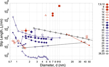
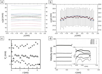
In nonequilibrium molecular dynamics (NEMD) simulations, an external force or a pressure gradient is applied to the water molecules along the axial direction. The streaming velocity profiles are analyzed to measure the slip velocity and slip length. The external forces used correspond to pressure differences three to four orders of magnitude higher than those used in typical experiments to achieve the required fluid velocities (generally above 10 m/s) and high signal-to-noise ratio within a few nanoseconds of simulated time. In Figure 2 , we compile the slip lengths reported in both experimental and simulation studies, which show a vast range of values extending almost six orders of magnitude. As can be seen from Figure 3 , ^{Reference Falk, Sedlmeier, Joly, Netz and Bocquet20,Reference Kannam, Todd, Hansen and Daivis31,Reference Hanasaki and Nakatani32} where we display some of the flow velocity profiles taken from the literature, the fluid velocity gradient is small. This weakness in the velocity gradient makes the slip length extraction difficult and unreliable.

Figure 2.

Slip length of water in carbon nanotubes. The results from experimental, simulation, and theoretical methods are shown in red, blue, and black, respectively. Reference numbers are given on the far right-hand side of the figure.

Figure 3.

Poiseuille flow velocity profiles of water in (a–b) graphene nanochannels and (c–d) carbon nanotubes (CNTs). Some of the velocity profiles in (a) are inverted parabolas due to the small difference in the velocity from channel center to the walls. (b) The quadratic fits to the average velocity profiles (in [a]) constrained by the shear viscosity (blue) and unconstrained fits (red). The slip length extracted from the fits differ by more than 100% due to the small gradient in the velocity profiles. ^{Reference Kannam, Todd, Hansen and Daivis31} (c–d) Non-quadratic nature of velocity profiles in CNTs. ^{Reference Falk, Sedlmeier, Joly, Netz and Bocquet20,Reference Hanasaki and Nakatani32} For more non-quadratic water velocity profiles in CNTs, please see References Reference Thomas and McGaughey17, Reference Joseph and Aluru19, Reference Falk, Sedlmeier, Joly, Netz and Bocquet20, Reference Kotsalis, Walther and Koumoutsakos23, and Reference Wang, Dumont and Dickson24.

Thomas et al. ^{Reference Thomas and McGaughey17} reassessed the results by Majumder et al. ^{Reference Majumder, Chopra, Andrews and Hinds7} and Holt et al., ^{Reference Holt, Park, Wang, Stadermann, Artyukhin, Grigoropoulos, Noy and Bakajin8} and hypothesized a miscalculation of the available flow area or the presence of an uncontrolled experimental variable (e.g., an electric field) in earlier experiments. For nanotubes of 1.66 to 4.99 nm diameter, they found slip lengths monotonically decreasing from 105 to 30 nm (433 to 47 enhancement). In a later study, they examined the fluid structure in narrow tubes of 0.83 to 1.66 nm diameter, and concluded that down to 1.39 nm diameter, the flow can be described by continuum theory by taking the slip into account. ^{Reference Thomas and McGaughey18} Below this tube diameter, the fluid becomes highly structured with no clear trend in the flow rate. For the smallest diameter (0.83 nm), their results suggest a slip length of 1000 nm and a flow enhancement of 5000.

Joseph et al. ^{Reference Joseph and Aluru19} conducted an investigation on the effects of nanotube smoothness and hydrophobicity, by varying the C–C bond distance (0.142 nm) and water–nanotube interaction strength. They concluded that a unique combination of features such as hexagonal structure, interatomic distances of 0.142 nm, and water orientations with “free” OH bonds pointing to the wall and decreased hydrogen bonding in the depletion region (only 5% bulk density near the wall surface) contribute to the large slip and flow rates of water in CNTs.

Babu et al. ^{Reference Babu and Sathian22} measured the activation energy required by water molecules to overcome the potential barrier along the flow direction. They attributed the enhanced flow rates in smaller tubes to the decrease in activation energy and shear viscosity (calculated using the Eyring theory). They also found that the flow enhancement decreased from 65 to 2 as the tube diameter increased from 0.83 to 5.42 nm.

Ma et al. ^{Reference Ma, Shen, Sheridan, Liu, Chen and Zheng21} found that for a 2.72-nm-diameter tube, slip lengths vary from 205 to 1120 nm with increasing contact angle, when the contact angle of water is varied from 45° to 135° through controlling the oxygen–carbon interaction strength. This indicated the importance of hydrophobicity on high slip. They proposed an inverse hyperbolic sine relationship between the water–CNT interfacial shear stress and slip velocity.

Myers ^{Reference Myers25} proposed a theoretical model based on a depletion layer with reduced viscosity near the wall. This model predicted a slip length of 8.57 nm for a 1.4-nm-diameter tube; as the diameter increased to 40 nm, the slip length approached 35 nm. He argued that describing the slip length as the length scale over which the fluid layer slips over the boundary or, to be more specific, as “the distance the velocity profile at the wall must be extrapolated to reach zero” is misleading when the slip length is larger than the tube diameter. Mattia et al. ^{Reference Mattia and Calabro26,Reference Ritos, Mattia, Calabro and Reese33} presented a model to predict the flow enhancement using the tube characteristic dimensions and fluid–wall interactions via the work of adhesion and surface diffusion. Their model suggests that the fluid velocity slip at the wall is solely a function of the fluid–wall interaction and is not a function of the tube characteristics or the pressure gradient, while the overall velocity profile depends on both.

In other studies, Du et al. ^{Reference Du, Qu, Xia, Feng and Dai11} found a slip length of 260 nm for a 4-nm-diameter tube; Nicholls et al. ^{Reference Nicholls, Borg, Lockerby and Reese13} found a slip length of 100 nm for a 0.96-nm-diameter tube; Kotsalis et al. ^{Reference Kotsalis34} found an increasing slip length of 11 to 15 nm as the tube diameter increased from 2.71 to 5.42 nm; and Wang et al. ^{Reference Wang, Dumont and Dickson24} found a slip length of only a few nanometers for tube diameters from 1.09 to 1.62 nm. Many other studies have focused on water flow and its transport properties in CNTs even though they have not explicitly reported the slip length or flow enhancement.

Equilibrium MD: Slip length from friction coefficient

Next, we briefly summarize two equilibrium MD methods ^{Reference Bocquet and Barrat35,Reference Kannam, Todd, Hansen and Daivis36} that have been used to calculate slip lengths for the system of water in CNTs. Other methods have been proposed, but not necessarily used for water in CNTs described here, and thus will not be discussed. ^{Reference Petravic and Harrowell37–Reference Bhadauria and Aluru41}

Bocquet and Barrat ^{Reference Bocquet and Barrat35} developed the first equilibrium MD-based method. They proposed a Green–Kubo type expression for the friction coefficient between the wall and the fluid. Falk et al. ^{Reference Falk, Sedlmeier, Joly, Netz and Bocquet20} used their method and found a slip length that monotonically decreased from 2600 to 120 nm when the tube diameter increased from 0.81 to 7 nm, respectively. They showed a structural origin, the curvature-induced incommensurability between the water and CNT, to be a potential origin of high slip.

Hansen et al. proposed another method ^{Reference Hansen, Todd and Daivis42} that explicitly takes into account only the local wall–fluid friction by separating out the viscous and frictional contributions. This method is not a Green–Kubo expression and does not rely on convergence of a time integral. Kannam et al. ^{Reference Kannam, Todd, Hansen and Daivis6,Reference Kannam, Todd, Hansen and Daivis31} demonstrated that the model of Hansen et al. was able to accurately predict the slip length for systems of water confined to planar graphene and CNTs. Their comparisons were done against NEMD simulations of these systems under flow conditions and excellent agreement was found: a monotonically decreasing slip length from 180 to 75 nm when the tube diameter increased from 1.62 to 6.5 nm. They concluded that NEMD simulations must be analyzed carefully for high slip systems such as water flowing in CNTs, otherwise large errors may result from extrapolated slip lengths. The equilibrium method was found to be much more reliable.